Numerical Methods I Monte Carlo Methodsdonev/Teaching/NMI-Fall2010/Lecture12.hand… · Numerical...

Numerical Methods IMonte Carlo Methods

Aleksandar DonevCourant Institute, NYU1

[email protected]

1Course G63.2010.001 / G22.2420-001, Fall 2010

Dec. 9th, 2010

A. Donev (Courant Institute) Lecture XII 12/09/2010 1 / 36

Outline

1 Background

2 Pseudo-Random NumbersInversion MethodRejectionHistogramming

3 Monte Carlo Integration

4 Conclusions


Logistics for Presentations

This is the last lecture: Dec. 16th is reserved for final presentationsand course evaluation forms.

We will start at 5pm sharp on Dec. 16th

Everyone should attend Dec. 16th as if a regular lecture.

Each presentation is only 15 minutes including questions: I willstrictly enforce this!

People presenting on the 16th (in alphabetical order): Cohen N.,Delong S., Guo S., Li X., Liu Y., Lopes D., Lu. L, Ye. S.

Email me PDF/PowerPoint of your presentation at least 1hbefore the scheduled talk time.

If you need to use your own laptop, explain why and still send me thefile.


Background

What is Monte Carlo?

Monte Carlo is any numerical algorithm that uses random numbers tocompute a deterministic (non-random) answer: stochastic orrandomized algorithm.

An important example is numerical integration in higherdimensions:

J =

∫Ω⊆Rn

f (x) dx

Recall that using a deterministic method is very accurate and fastfor low dimensions.

But for large dimensions we have to deal with the curse ofdimensionality:The number of quadrature nodes scales like at least 2n

(exponentially). E.g., 220 = 106, but 240 = 1012!


Background

Probability Theory

First define a set Ω of possible outcomes ω ∈ Ω of an “experiment”:

A coin toss can end in heads or tails, so two outcomes.A sequence of four coin tosses can end in one of 42 = 16 outcomes,e.g., HHTT or THTH.

The set Ω can be finite (heads or tails), countably infinite (the numberof atoms inside a box), or uncountable (the weight of a person).

An event A ⊆ Ω is a set of possible outcomes: e.g., more tailsthen heads occur in a sequence of four coin tosses,

A = HHHH,THHH,HTHH,HHTH,HHHT .

Each event has an associated probability

0 ≤ P(A) ≤ 1,

with P(Ω) = 1 and P(∅) = 0.


Background

Conditional Probability

A basic axiom is that probability is additive for disjoint events:

P (A ∪ B) = P (A or B) = P (A) + P (B) if A ∩ B = ∅

Bayes formula gives the conditional probability that an outcomebelongs to set B if it belongs to set C :

P (B|C ) =P (B ∩ C )

P (C )=

P (B and C )

P (C )

Two events are said to be independent if their probabilities aremultiplicative:

P (A ∩ B) = P (A and B) = P (A)P (B)

When the set of all outcomes is countable, we can associate witheach event a probability, and then

P (A) =∑ωi∈A

P (ωi ) .


Background

Probability Distribution

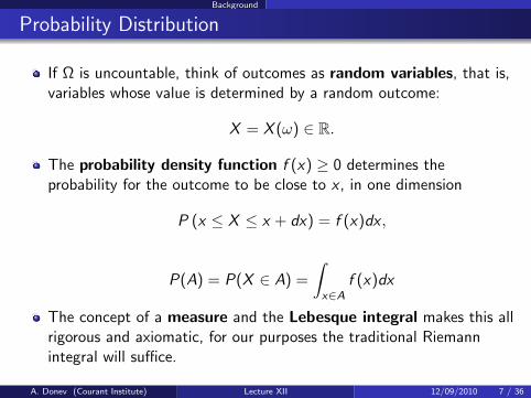
If Ω is uncountable, think of outcomes as random variables, that is,variables whose value is determined by a random outcome:

X = X (ω) ∈ R.

The probability density function f (x) ≥ 0 determines theprobability for the outcome to be close to x , in one dimension

P (x ≤ X ≤ x + dx) = f (x)dx ,

P(A) = P(X ∈ A) =

∫x∈A

f (x)dx

The concept of a measure and the Lebesque integral makes this allrigorous and axiomatic, for our purposes the traditional Riemannintegral will suffice.


Background

Mean and Variance

We call the probability density or the probability measure the lawor the distribution of a random variable X , and write:

X ∼ f .

The cummulative distribution function is

F (x) = P(X ≤ x) =

∫ x

−∞f (x ′)dx ′,

and we will assume that this function is continuous.The mean or expectation value of a random variable X is

µ = X = E [X ] =

∫ ∞−∞

xf (x)dx .

The variance σ2 and the standard deviation σ measure theuncertainty in a random variable

σ2 = var(X ) = E [(X − µ)2] =

∫ ∞−∞

(x − µ)2f (x)dx .


Background

Multiple Random Variables

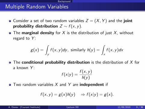
Consider a set of two random variables Z = (X ,Y ) and the jointprobability distribution Z ∼ f (x , y).

The marginal density for X is the distribution of just X , withoutregard to Y :

g(x) =

∫yf (x , y)dy , similarly h(y) =

∫xf (x , y)dx

The conditional probability distribution is the distribution of X fora known Y :

f (x |y) =f (x , y)

h(y)

Two random variables X and Y are independent if

f (x , y) = g(x)h(y) ⇒ f (x |y) = g(x).


Background

Covariance

The term i.i.d.≡independent identically-distributed randomvariables is used to describe independent samples Xk ∼ f , k = 1, . . . .

The generalization of variance for two variables is the covariance:

CXY = cov(X ,Y ) = E[(X − X

) (Y − Y

)]= E (XY )− E (X )E (Y ).

For independent variables

E (XY ) =

∫xy f (x , y)dxdy =

∫xg(x)dx

∫yh(y)dy = E (X )E (Y )

and so CXY = 0.

Define the correlation coefficient between X and Y as a measure ofhow correlated two variables are:

rXY =cov(X ,Y )√var(X )var(Y )

=CXY

σXσY.


Background

Law of Large Numbers

The average of N i.i.d. samples of a random variable X ∼ f is itself arandom variable:

A =1

N

N∑k=1

Xk .

A is an unbiased estimator of the mean of X , E (A) = X .

Numerically we often use a biased estimate of the variance:

σ2X = lim

N→∞

1

N

N∑k=1

(Xk − X

)2 ≈ 1

N

N∑k=1

(Xk − A)2 .

The weak law of large numbers states that the estimator is alsoconsistent:

limN→∞

A = X = E (X ) (almost surely).


Background

Central Limit Theorem

The central value theorem says that if σX is finite, in the limitN →∞ the random variable A is normally-distributed:

A ∼ f (a) =(2πσ2

A

)−1/2exp

[−(a− X )2

2σ2A

]The error of the estimator A decreases as N−1, more specifically,

E[(A− X

)2]

= E

[

1

N

N∑k=1

(Xk − X

)]2 =

1

N2E

[N∑

k=1

(Xk − X

)2

]

var(A) = σ2A =

σ2X

N.

The slow convergence of the error, σ ∼ N−1/2, is a fundamentalcharacteristic of Monte Carlo.


Pseudo-Random Numbers

Monte Carlo on a Computer

In order to compute integrals using Monte Carlo on a computer, weneed to be able to generate samples from a distribution, e.g.,uniformly distributed inside an interval I = [a, b].

Almost all randomized software is based on having a pseudo-randomnumber generator (PRNG), which is a routine that returns apseudo-random number 0 ≤ u ≤ 1 from the standard uniformdistribution:

f (u) =

1 if 0 ≤ u ≤ 1

0 otherwise

Since computers (Turing machines) are deterministic, it is notpossible to generate truly random samples (outcomes):Pseudo-random means as close to random as we can get it.

There are well-known good PRNGs that are also efficient: One shoulduse other-people’s PRNGs, e.g., the Marsenne Twister.



PRNGs

The PRNG is a procedure (function) that takes a collection of mintegers called the state of the generator s = i1, . . . , im, andupdates it:

s← Φ(s),

and produces (returns) a number u = Ψ(s) that is a pseudo-randomsample from the standard uniform distribution.

So in pseudo-MATLAB notation, [u, s] = rng(s), often called arandom stream.

Simple built-in generator such as the MATLAB/C function rand orthe Fortran function RANDOM NUMBER hide the state from theuser (but the state is stored somewhere in some global variable).

All PRNGs provide a routine to seed the generator, that is, to setthe seed s to some particular value.This way one can generate the same sequence of “random” numbersover and over again (e.g., when debugging a program).



Generating Non-Uniform Variates

Using a uniform (pseudo-)random number generator (URNG), it iseasy to generate an outcome drawn uniformly in I = [a, b]:

X = a + (b − a)U,

where U = rng() is a standard uniform variate.

We often need to generate (pseudo)random samples or variatesdrawn from a distribution other than a uniform distribution.

Almost all non-uniform samplers are based on a URNG.

Sometimes it may be more efficient to replace the URNG with arandom bitstream, that is, a sequence of random bits, if only a fewrandom bits are needed (e.g., for discrete variables).

We need a method to convert a uniform variate into a non-uniformvariate.



Generating Non-Uniform Variates

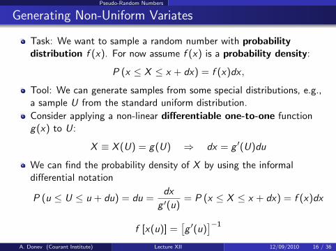
Task: We want to sample a random number with probabilitydistribution f (x). For now assume f (x) is a probability density:

P (x ≤ X ≤ x + dx) = f (x)dx ,

Tool: We can generate samples from some special distributions, e.g.,a sample U from the standard uniform distribution.

Consider applying a non-linear differentiable one-to-one functiong(x) to U:

X ≡ X (U) = g(U) ⇒ dx = g ′(U)du

We can find the probability density of X by using the informaldifferential notation

P (u ≤ U ≤ u + du) = du =dx

g ′(u)= P (x ≤ X ≤ x + dx) = f (x)dx

f [x(u)] =[g ′(u)

]−1


Pseudo-Random Numbers Inversion Method

Inverting the CDF

f [x(u)] =[g ′(u)

]−1

Can we find g(u) given the target f (x)? It is simpler to see this if weinvert x(u):

u = F (x).

Repeating the same calculation

P (u ≤ U ≤ u + dx) = du = F ′(x)dx = f (x)dx

F ′(x) = f (x)

This shows that F (x) is the cummulative probability distribution:

F (x) = P(X ≤ x) =

∫ x

−∞f (x ′)dx ′.

Note that F (x) is monotonically non-decreasing because f (x) ≥ 0.Still it is not always easy to invert the CDF efficiently.



Sampling by Inversion

Generate a standard uniform variate u and then solve the non-linearequation F (x) = u. If F (x) has finite jumps just think of u as theindependent variable instead of x .



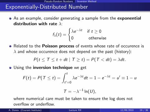
Exponentially-Distributed Number

As an example, consider generating a sample from the exponentialdistribution with rate λ:

fλ(t) =

λe−λt if t ≥ 0

0 otherwise

Related to the Poisson process of events whose rate of occurence isλ and whose occurence does not depend on the past (history):

P(t ≤ T ≤ t + dt | T ≥ t) = P(T < dt) = λdt.

Using the inversion technique we get

F (t) = P(T ≤ t) =

∫ t

t′=0λe−λtdt = 1− e−λt = u′ ≡ 1− u

T = −λ−1 ln(U),

where numerical care must be taken to ensure the log does notoverflow or underflow.


Pseudo-Random Numbers Rejection

Rejection Sampling

An alternative method is to use rejection sampling:Generate a sample X from some other distribution g(x) and acceptthem with acceptance probability p(X ), otherwise reject and tryagain.

The rejection requires sampling a standard uniform variate U:Accept if U ≤ p(X ), reject otherwise.

It is easy to see that

f (x) ∼ g(x)p(x) ⇒ p(x) = Zf (x)

g(x),

where Z is determined from the normalization condition:∫f (x)dx = 1 ⇒

∫p(x)g(x) = Z



Envelope Function

p(x) =f (x)

Z−1g(x)=

f (x)

g(x)

Since 0 ≤ p(x) ≤ 1, we see that g(x) = Z−1g(x) must be abounding or envelope function:

g(x) ≥ f (x), for example, g(x) = max f (x) = const.

Rejection sampling is very simple:Generate a sample X from g(x) and a standard uniform variate Uand accept X if Ug(x) ≤ f (x), reject otherwise and try again.

For efficiency, we want to have the highest possible acceptanceprobability, that is

Pacc =

∫f (x)dx∫g(x)dx

= Z

∫f (x)dx∫g(x)dx

= Z .



Rejection Sampling Illustrated



Normally-Distributed Numbers

The standard normal distribution is a Gaussian “bell-curve”:

f (x) =(2πσ2

)−1/2exp

(−(x − µ)2

2σ2

),

where µ is the mean and σ is the standard deviation.

The standard normal distribution has σ = 1 and µ = 0.

If we have a sample Xs from the standard distribution we cangenerate a sample X from f (x) using:

X = µ+ σXs

Consider sampling the positive half of the standard normal, that is,sampling:

f (x) =

√2

πe−x

2/2 for x ≥ 0



Optimizing Rejection Sampling

We want the tighest possible (especially where f (x) is large)easy-to-sample g(x) ≈ f (x).

We already know how to sample an exponential:

g(x) = e−x

We want the tightest possible g(x):

min [g(x)− f (x)] = min

[Z−1e−x −

√2

πe−x

2/2

]= 0

g ′(x?) = f ′(x?) and g(x?) = f (x?)

Solving this system of two equations gives x? = 1 and

Z = Pacc =

√π

2e−1/2 ≈ 76%


Pseudo-Random Numbers Histogramming

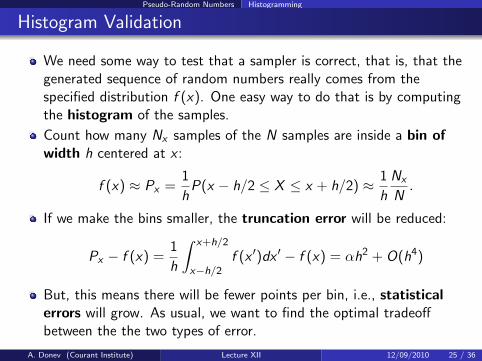
Histogram Validation

We need some way to test that a sampler is correct, that is, that thegenerated sequence of random numbers really comes from thespecified distribution f (x). One easy way to do that is by computingthe histogram of the samples.

Count how many Nx samples of the N samples are inside a bin ofwidth h centered at x :

f (x) ≈ Px =1

hP(x − h/2 ≤ X ≤ x + h/2) ≈ 1

h

Nx

N.

If we make the bins smaller, the truncation error will be reduced:

Px − f (x) =1

h

∫ x+h/2

x−h/2f (x ′)dx ′ − f (x) = αh2 + O(h4)

But, this means there will be fewer points per bin, i.e., statisticalerrors will grow. As usual, we want to find the optimal tradeoffbetween the the two types of error.



Statistical Error in Histogramming

For every sample point X , define the indicator random variable Y :

Y = Ix(X ) =

1 if x − h/2 ≤ X ≤ x + h/2

0 otherwise

The mean and variance of this Bernoulli random variable are:

E (Y ) = Y = hPx ≈ hf (x)

σ2Y =

∫(y − Y )2f (y)dy = Y · (1− Y ) ≈ Y ≈ hf (x)

The number Nx out of N trials inside the bin is a sum of N randomBernoulli variables Yi :

f (x) ≈ 1

h

Nx

N= h−1

(1

N

N∑i=1

Yi

)= Px



Optimal Bin Width

The central limit theorem says

σ(Px) ≈ h−1 σY√N

=

√f (x)

hN

The optimal bin width is when the truncation and statistical errors areequal:

h2 ∼√

1

hN⇒ h ∼ N−1/5,

with total error ε ∼ (hN)−1/2 ∼ N−2/5.

This is because statistical errors dominate and so using a larger binis better...unless there are small-scale features in f (x) that need tobe resolved.


Monte Carlo Integration

Integration via Monte Carlo

Define the random variable Y = f (X), and generate a sequence of Nindependent uniform samples Xk ∈ Ω, i.e., N random variablesdistributed uniformly inside Ω:

X ∼ g(x) =

|Ω|−1 for x ∈ Ω

0 otherwise

and calculate the mean

Y =1

N

N∑k=1

Yk =1

N

N∑k=1

f (Xk)

According to the weak law of large numbers,

limN→∞

Y = E (Y ) = Y =

∫f (x)g(x)dx = |Ω|−1

∫Ωf (x) dx



Accuracy of Monte Carlo Integration

This gives a Monte Carlo approximation to the integral:

J =

∫Ω∈Rn

f (x) dx = |Ω| Y ≈ |Ω| Y = |Ω| 1

N

N∑k=1

f (Xk) .

Recalling the central limit theorem, for large N we get an errorestimate by evaluating the standard deviation of the estimate Y :

σ2(Y)≈σ2Y

N= N−1

∫Ω

[f (x)− |Ω|−1 J

]2dx

σ(Y)≈ 1√

N

[∫Ω

[f (x)− f (x)

]2dx

]1/2

Note that this error goes like N−1/2, which is order of convergence1/2: Worse than any deterministic quadrature.

But, the same number of points are needed to get a certain accuracyindependent of the dimension.



Integration by Rejection

Note how this becomes lessefficient as dimension grows(most points are outside thesphere).

Integration requires |Ω|:∫Ω∈Rn

f (x) dx ≈ |Ω| 1

N

N∑k=1

f (Xk)

Consider Ω being the unit circle ofradius 1.

Rejection: Integrate by samplingpoints inside an enclosing region,e.g, a square of area |Ωencl | = 4, andrejecting any points outside of Ω:∫

Ω∈Rn

f (x) dx ≈ |Ωencl |1

N

∑Xk∈Ω

f (Xk)



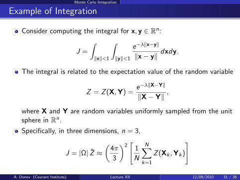
Example of Integration

Consider computing the integral for x, y ∈ Rn:

J =

∫‖x‖<1

∫‖y‖<1

e−λ‖x−y‖

‖x− y‖dxdy.

The integral is related to the expectation value of the random variable

Z = Z (X,Y) =e−λ‖X−Y‖

‖X− Y‖,

where X and Y are random variables uniformly sampled from the unitsphere in Rn.

Specifically, in three dimensions, n = 3,

J = |Ω| Z ≈(

4π

3

)2[

1

N

N∑k=1

Z (Xk ,Yk)

]



Variance Reduction

Recall that the standard deviation of the Monte Carlo estimate for theintegral is:

σ(Y)≈ 1√

N

[∫Ω

[f (x)− f (x)

]2dx

]1/2

Since the answer is approximately normally-distributed, we have thewell-known confidence intervals:

P

(J

|Ω|∈[Y − σ, Y + σ

])≈ 66%

P

(J

|Ω|∈[Y − 2σ, Y + 2σ

])≈ 95%

The most important thing in Monte Carlo is variance reduction, i.e.,finding methods that give the same answers in the limit N →∞ buthave a much smaller σ.



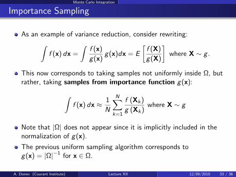
Importance Sampling

As an example of variance reduction, consider rewriting:∫f (x) dx =

∫f (x)

g(x)g(x)dx = E

[f (X)

g(X)

]where X ∼ g .

This now corresponds to taking samples not uniformly inside Ω, butrather, taking samples from importance function g(x):∫

f (x) dx ≈ 1

N

N∑k=1

f (Xk)

g (Xk)where X ∼ g

Note that |Ω| does not appear since it is implicitly included in thenormalization of g(x).

The previous uniform sampling algorithm corresponds tog(x) = |Ω|−1 for x ∈ Ω.



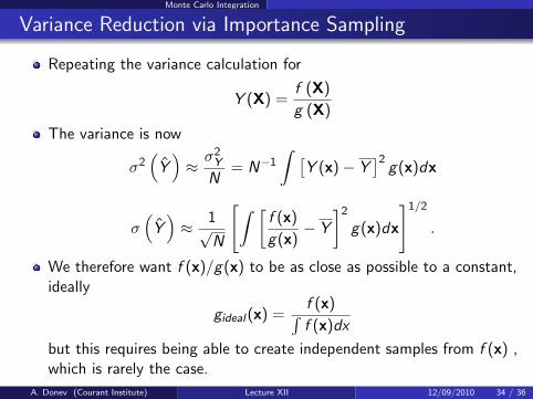
Variance Reduction via Importance Sampling

Repeating the variance calculation for

Y (X) =f (X)

g (X)

The variance is now

σ2(Y)≈σ2Y

N= N−1

∫ [Y (x)− Y

]2g(x)dx

σ(Y)≈ 1√

N

[∫ [f (x)

g(x)− Y

]2

g(x)dx

]1/2

.

We therefore want f (x)/g(x) to be as close as possible to a constant,ideally

gideal(x) =f (x)∫f (x)dx

but this requires being able to create independent samples from f (x) ,which is rarely the case.



Importance Sampling Example

Consider again computing:

J =

∫‖x‖<1

∫‖y‖<1

e−λ‖x−y‖

‖x− y‖dxdy.

The standard Monte Carlo will have a large variance because of thesingularity when x = y:The integrand is very non-uniform around the singularity.

If one could sample from the distribution

g(x, y) ∼ 1

‖x− y‖when x ≈ y,

then the importance function will capture the singularity and thevariance will be greatly reduced.


Conclusions

Conclusions/Summary

Monte Carlo is an umbrella term for stochastic computation ofdeterministic answers.

Monte Carlo answers are random, and their accuracy is measured bythe variance or uncertaintly of the estimate, which typically scaleslike σ ∼ N−1/2, where N is the number of samples.

Implementing Monte Carlo algorithms on a computer requires aPRNG, almost always a uniform pseudo-random numbergenerator (URNG).

One often needs to convert a sample from a URNG to a sample froman arbitrary distribution f (x), including inverting the cummulativedistribution and rejection sampling.

Monte Carlo can be used to perform integration in high dimensionsby simply evaluating the function at random points.

Variance reduction is the search for algorithms that give the sameanswer but with less statistical error. One example is importancesampling.


Numerical Methods I Monte Carlo Methodsdonev/Teaching/NMI-Fall2010/Lecture12.hand… · Numerical...

Documents

Transcript of Numerical Methods I Monte Carlo Methodsdonev/Teaching/NMI-Fall2010/Lecture12.hand… · Numerical...