Numerical Methods I Mathematical Programming...

Numerical Methods IMathematical Programming (Optimization)

Aleksandar DonevCourant Institute, NYU1

[email protected]

1MATH-GA 2011.003 / CSCI-GA 2945.003, Fall 2014

October 23rd, 2014

A. Donev (Courant Institute) Lecture VII 10/2014 1 / 30

Outline

1 Mathematical Background

2 Smooth Unconstrained Optimization

3 Constrained Optimization

4 Conclusions


Mathematical Background

Formulation

Optimization problems are among the most important in engineeringand finance, e.g., minimizing production cost, maximizing profits,etc.

minx∈Rn

f (x)

where x are some variable parameters and f : Rn → R is a scalarobjective function.

Observe that one only need to consider minimization as

maxx∈Rn

f (x) = − minx∈Rn

[−f (x)]

A local minimum x? is optimal in some neighborhood,

f (x?) ≤ f (x) ∀x s.t. ‖x− x?‖ ≤ R > 0.

(think of finding the bottom of a valley)

Finding the global minimum is generally not possible for arbitraryfunctions (think of finding Mt. Everest without a satelite).



Connection to nonlinear systems

Assume that the objective function is differentiable (i.e., first-orderTaylor series converges or gradient exists).

Then a necessary condition for a local minimizer is that x? be acritical point

g (x?) = ∇xf (x?) =

{∂f

∂xi(x?)

}i

= 0

which is a system of non-linear equations!

In fact similar methods, such as Newton or quasi-Newton, apply toboth problems.

Vice versa, observe that solving f (x) = 0 is equivalent to anoptimization problem

minx

[f (x)T f (x)

]although this is only recommended under special circumstances.



Sufficient Conditions

Assume now that the objective function is twice-differentiable (i.e.,Hessian exists).

A critical point x?is a local minimum if the Hessian is positivedefinite

H (x?) = ∇2xf (x?) � 0

which means that the minimum really looks like a valley or a convexbowl.

At any local minimum the Hessian is positive semi-definite,∇2

xf (x?) � 0.

Methods that require Hessian information converge fast but areexpensive (next class).



Mathematical Programming

The general term used is mathematical programming.

Simplest case is unconstrained optimization

minx∈Rn

f (x)

where x are some variable parameters and f : Rn → R is a scalarobjective function.

Find a local minimum x?:

f (x?) ≤ f (x) ∀x s.t. ‖x− x?‖ ≤ R > 0.

(think of finding the bottom of a valley).Find the best local minimum, i.e., the global minimumx?: This isvirtually impossible in general and there are many specializedtechniques such as genetic programming, simmulated annealing,branch-and-bound (e.g., using interval arithmetic), etc.

Special case: A strictly convex objective function has a uniquelocal minimum which is thus also the global minimum.



Constrained Programming

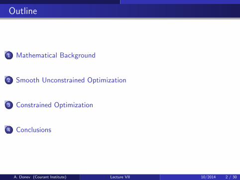
The most general form of constrained optimization

minx∈X

f (x)

where X ⊂ Rn is a set of feasible solutions.

The feasible set is usually expressed in terms of equality andinequality constraints:

h(x) = 0

g(x) ≤ 0

The only generally solvable case: convex programmingMinimizing a convex function f (x) over a convex set X : every localminimum is global.If f (x) is strictly convex then there is a unique local and globalminimum.



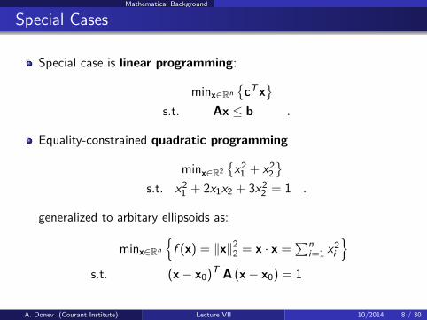
Special Cases

Special case is linear programming:

minx∈Rn

{cTx

}s.t. Ax ≤ b .

Equality-constrained quadratic programming

minx∈R2

{x21 + x22

}s.t. x21 + 2x1x2 + 3x22 = 1 .

generalized to arbitary ellipsoids as:

minx∈Rn

{f (x) = ‖x‖22 = x · x =

∑ni=1 x

2i

}s.t. (x− x0)T A (x− x0) = 1


Smooth Unconstrained Optimization

Necessary and Sufficient Conditions

A necessary condition for a local minimizer:The optimum x? must be a critical point (maximum, minimum orsaddle point):

g (x?) = ∇xf (x?) =

{∂f

∂xi(x?)

}i

= 0,

and an additional sufficient condition for a critical point x? to be alocal minimum:The Hessian at the optimal point must be positive definite,

H (x?) = ∇2xf (x?) =

{∂2f

∂xi∂xj(x?)

}ij

� 0.

which means that the minimum really looks like a valley or a convexbowl.



Direct-Search Methods

A direct search method only requires f (x) to be continuous butnot necessarily differentiable, and requires only function evaluations.

Methods that do a search similar to that in bisection can be devisedin higher dimensions also, but they may fail to converge and areusually slow.

The MATLAB function fminsearch uses the Nelder-Mead orsimplex-search method, which can be thought of as rolling a simplexdownhill to find the bottom of a valley. But there are many othersand this is an active research area.

Curse of dimensionality: As the number of variables(dimensionality) n becomes larger, direct search becomes hopelesssince the number of samples needed grows as 2n!



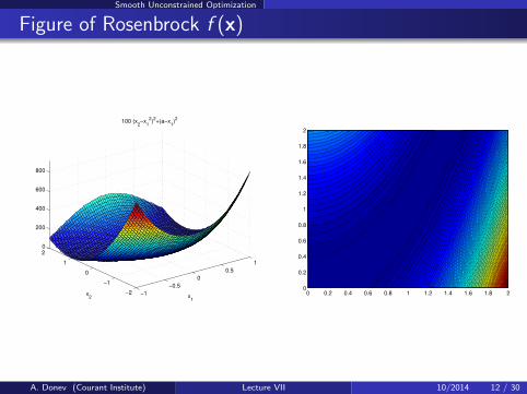
Minimum of 100(x2 − x21 )2 + (a − x1)2 in MATLAB

% Rosenbrock or ’ banana ’ f u n c t i o n :a = 1 ;banana = @( x ) 100∗( x (2)−x (1)ˆ2)ˆ2+(a−x ( 1 ) ) ˆ 2 ;

% This f u n c t i o n must accep t a r r a y arguments !banana xy = @( x1 , x2 ) 100∗( x2−x1 .ˆ2) . ˆ2+( a−x1 ) . ˆ 2 ;

f i g u r e ( 1 ) ; e z s u r f ( banana xy , [ 0 , 2 , 0 , 2 ] )

[ x , y ] = meshgrid ( l i n s p a c e ( 0 , 2 , 1 0 0 ) ) ;f i g u r e ( 2 ) ; c o n t ou r f ( x , y , banana xy ( x , y ) , 100)

% Cor r e c t answers a r e x =[1 ,1 ] and f ( x)=0[ x , f v a l ] = fm in s e a r ch ( banana , [−1.2 , 1 ] , op t imse t ( ’ TolX ’ ,1 e−8))x = 0.999999999187814 0.999999998441919f v a l = 1.099088951919573 e−18



Figure of Rosenbrock f (x)

−1

−0.5

0

0.5

1

−2

−1

0

1

20

200

400

600

800

x1

100 (x2−x

1

2)2+(a−x

1)2

x2

0 0.2 0.4 0.6 0.8 1 1.2 1.4 1.6 1.8 20

0.2

0.4

0.6

0.8

1

1.2

1.4

1.6

1.8

2



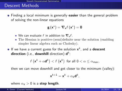
Descent Methods

Finding a local minimum is generally easier than the general problemof solving the non-linear equations

g (x?) = ∇xf (x?) = 0

We can evaluate f in addition to ∇xf .The Hessian is positive-(semi)definite near the solution (enablingsimpler linear algebra such as Cholesky).

If we have a current guess for the solution xk , and a descentdirection (i.e., downhill direction) dk :

f(xk + αdk

)< f

(xk)

for all 0 < α ≤ αmax ,

then we can move downhill and get closer to the minimum (valley):

xk+1 = xk + αkdk ,

where αk > 0 is a step length.



Gradient Descent Methods

For a differentiable function we can use Taylor’s series:

f(xk + αdk

)≈ f

(xk)

+ αk

[(∇f )T dk

]This means that fastest local decrease in the objective is achievedwhen we move opposite of the gradient: steepest or gradientdescent:

dk = −∇f(xk)

= −gk .

One option is to choose the step length using a line searchone-dimensional minimization:

αk = arg minα

f(xk + αdk

),

which needs to be solved only approximately.



Steepest Descent

Assume an exact line search was used, i.e., αk = arg minα φ(α) where

φ(α) = f(xk + αdk

).

φ′(α) = 0 =[∇f

(xk + αdk

)]Tdk .

This means that steepest descent takes a zig-zag path down to theminimum.

Second-order analysis shows that steepest descent has linearconvergence with convergence coefficient

C ∼ 1− r

1 + r, where r =

λmin (H)

λmax (H)=

1

κ2(H),

inversely proportional to the condition number of the Hessian.

Steepest descent can be very slow for ill-conditioned Hessians: Oneimprovement is to use conjugate-gradient method instead (seebook).



Newton’s Method

Making a second-order or quadratic model of the function:

f (xk + ∆x) = f (xk) +[g(xk)]T

(∆x) +1

2(∆x)T

[H(xk)]

(∆x)

we obtain Newton’s method:

g(x + ∆x) = ∇f (x + ∆x) = 0 = g + H (∆x) ⇒

∆x = −H−1g ⇒ xk+1 = xk −[H(xk)]−1 [

g(xk)].

Note that this is exact for quadratic objective functions, whereH ≡ H

(xk)

= const.

Also note that this is identical to using the Newton-Raphson methodfor solving the nonlinear system ∇xf (x?) = 0.



Problems with Newton’s Method

Newton’s method is exact for a quadratic function and converges inone step!

For non-linear objective functions, however, Newton’s method requiressolving a linear system every step: expensive.

It may not converge at all if the initial guess is not very good, or mayconverge to a saddle-point or maximum: unreliable.

All of these are addressed by using variants of quasi-Newtonmethods:

xk+1 = xk − αkH−1k

[g(xk)],

where 0 < αk < 1 and Hk is an approximation to the true Hessian.


Constrained Optimization

General Formulation

Consider the constrained optimization problem:

minx∈Rn f (x)

s.t. h(x) = 0 (equality constraints)

g(x) ≤ 0 (inequality constraints)

Note that in principle only inequality constraints need to beconsidered since

h(x) = 0 ≡

{h(x) ≤ 0

h(x) ≥ 0

but this is not usually a good idea.

We focus here on non-degenerate cases without considering variouscomplications that may arrise in practice.



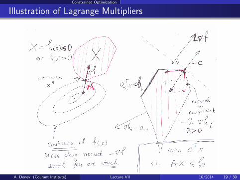
Illustration of Lagrange Multipliers



Linear Programming

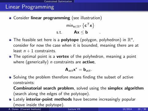
Consider linear programming (see illustration)

minx∈Rn

{cTx

}s.t. Ax ≤ b .

The feasible set here is a polytope (polygon, polyhedron) in Rn,consider for now the case when it is bounded, meaning there are atleast n + 1 constraints.The optimal point is a vertex of the polyhedron, meaning a pointwhere (generically) n constraints are active,

Aactx? = bact .

Solving the problem therefore means finding the subset of activeconstraints:Combinatorial search problem, solved using the simplex algorithm(search along the edges of the polytope).Lately interior-point methods have become increasingly popular(move inside the polytope).



Lagrange Multipliers: Single equality

An equality constraint h(x) = 0 corresponds to an(n − 1)−dimensional constraint surface whose normal vector is ∇h.

The illustration on previous slide shows that for a single smoothequality constraint, the gradient of the objective function must beparallel to the normal vector of the constraint surface:

∇f ‖ ∇h ⇒ ∃λ s.t. ∇f + λ∇h = 0,

where λ is the Lagrange multiplier corresponding to the constrainth(x) = 0.

Note that the equation ∇f + λ∇h = 0 is in addition to theconstraint h(x) = 0 itself.



Lagrange Multipliers: m equalities

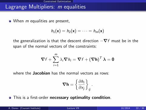
When m equalities are present,

h1(x) = h2(x) = · · · = hm(x)

the generalization is that the descent direction −∇f must be in thespan of the normal vectors of the constraints:

∇f +m∑i=1

λi∇hi = ∇f + (∇h)T λ = 0

where the Jacobian has the normal vectors as rows:

∇h =

{∂hi∂xj

}ij

.

This is a first-order necessary optimality condition.



Lagrange Multipliers: Single inequalities

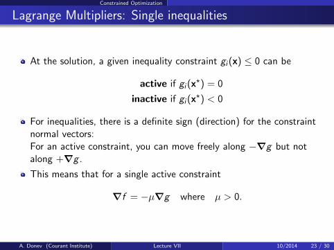
At the solution, a given inequality constraint gi (x) ≤ 0 can be

active if gi (x?) = 0

inactive if gi (x?) < 0

For inequalities, there is a definite sign (direction) for the constraintnormal vectors:For an active constraint, you can move freely along −∇g but notalong +∇g .

This means that for a single active constraint

∇f = −µ∇g where µ > 0.



Lagrange Multipliers: r inequalities

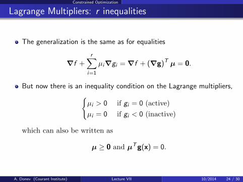
The generalization is the same as for equalities

∇f +r∑

i=1

µi∇gi = ∇f + (∇g)T µ = 0.

But now there is an inequality condition on the Lagrange multipliers,{µi > 0 if gi = 0 (active)

µi = 0 if gi < 0 (inactive)

which can also be written as

µ ≥ 0 and µTg(x) = 0.



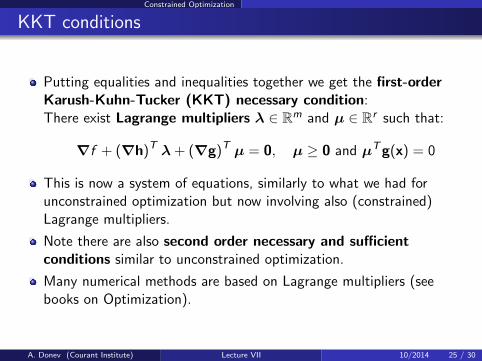
KKT conditions

Putting equalities and inequalities together we get the first-orderKarush-Kuhn-Tucker (KKT) necessary condition:There exist Lagrange multipliers λ ∈ Rm and µ ∈ Rr such that:

∇f + (∇h)T λ + (∇g)T µ = 0, µ ≥ 0 and µTg(x) = 0

This is now a system of equations, similarly to what we had forunconstrained optimization but now involving also (constrained)Lagrange multipliers.

Note there are also second order necessary and sufficientconditions similar to unconstrained optimization.

Many numerical methods are based on Lagrange multipliers (seebooks on Optimization).



Lagrangian Function

∇f + (∇h)T λ + (∇g)T µ = 0

We can rewrite this in the form of stationarity conditions

∇xL = 0

where L is the Lagrangian function:

L (x,λ,µ) = f (x) +m∑i=1

λihi (x) +r∑

i=1

µigi (x)

L (x,λ,µ) = f (x) + λT [h(x)] + µT [g(x)]



Equality Constraints

The first-order necessary conditions for equality-constrainedproblems are thus given by the stationarity conditions:

∇xL (x?,λ?) = ∇f (x?) + [∇h(x?)]T λ? = 0

∇λL (x?,λ?) = h(x?) = 0

Note there are also second order necessary and sufficientconditions similar to unconstrained optimization.

It is important to note that the solution (x?,λ?) is not a minimum ormaximum of the Lagrangian (in fact, for convex problems it is asaddle-point, min in x, max in λ).

Many numerical methods are based on Lagrange multipliers but we donot discuss it here.



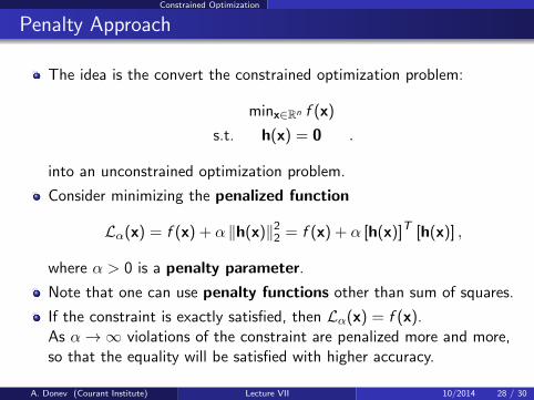
Penalty Approach

The idea is the convert the constrained optimization problem:

minx∈Rn f (x)

s.t. h(x) = 0 .

into an unconstrained optimization problem.

Consider minimizing the penalized function

Lα(x) = f (x) + α ‖h(x)‖22 = f (x) + α [h(x)]T [h(x)] ,

where α > 0 is a penalty parameter.

Note that one can use penalty functions other than sum of squares.

If the constraint is exactly satisfied, then Lα(x) = f (x).As α→∞ violations of the constraint are penalized more and more,so that the equality will be satisfied with higher accuracy.



Penalty Method

The above suggest the penalty method (see homework):For a monotonically diverging sequence α1 < α2 < · · · , solve asequence of unconstrained problems

xk = x (αk) = arg minx

{Lk(x) = f (x) + αk [h(x)]T [h(x)]

}and the solution should converge to the optimum x?,

xk → x? = x (αk →∞) .

Note that one can use xk−1 as an initial guess for, for example,Newton’s method.

Also note that the problem becomes more and more ill-conditioned asα grows.A better approach uses Lagrange multipliers in addition to penalty(augmented Lagrangian).


Conclusions

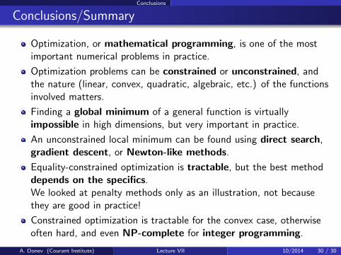
Conclusions/Summary

Optimization, or mathematical programming, is one of the mostimportant numerical problems in practice.

Optimization problems can be constrained or unconstrained, andthe nature (linear, convex, quadratic, algebraic, etc.) of the functionsinvolved matters.

Finding a global minimum of a general function is virtuallyimpossible in high dimensions, but very important in practice.

An unconstrained local minimum can be found using direct search,gradient descent, or Newton-like methods.

Equality-constrained optimization is tractable, but the best methoddepends on the specifics.We looked at penalty methods only as an illustration, not becausethey are good in practice!

Constrained optimization is tractable for the convex case, otherwiseoften hard, and even NP-complete for integer programming.


Numerical Methods I Mathematical Programming...

Documents

Transcript of Numerical Methods I Mathematical Programming...