Numerical Methods for the Root Finding Problem -...
66
Chapter 1 Numerical Methods for the Root Finding Problem Oct. 11, 2011 HG 1.1 A Case Study on the Root-Finding Problem: Kepler’s Law of Planetary Motion The root-finding problem is one of the most important computational problems. It arises in a wide variety of practical applications in physics, chemistry, biosciences, engineering, etc. As a matter of fact, determination of any unknown appearing implicitly in scientific or engineering formulas gives rise to a root-finding problem. We consider one such simple application here. One of the classical laws of planetary motion due to Kepler says that a planet revolves around the sun in an elliptic orbit as shown in the figure below : Suppose one needs to find the position (x, y) of the planet at time t. This can be determined by the following formula: x = a cos(E − e) y = a √ 1 − e 2 sin E where e = The eccentricity of the Ellipse E = Eccentric anomaly 1
Transcript of Numerical Methods for the Root Finding Problem -...
Chapter 1
Numerical Methods for the Root
Finding Problem
Oct. 11, 2011 HG
1.1 A Case Study on the Root-Finding Problem: Kepler’s Law
of Planetary Motion
The root-finding problem is one of the most important computational problems. It arises in
a wide variety of practical applications in physics, chemistry, biosciences, engineering,
etc. As a matter of fact, determination of any unknown appearing implicitly in scientific
or engineering formulas gives rise to a root-finding problem. We consider one such simple
application here.
One of the classical laws of planetary motion due to Kepler says that a planet revolves around
the sun in an elliptic orbit as shown in the figure below :
Suppose one needs to find the position (x, y) of the planet at time t. This can be determined
by the following formula:
x = a cos(E − e)
y = a√1− e2 sinE
where
e = The eccentricity of the Ellipse
E = Eccentric anomaly
1

2 CHAPTER 1. NUMERICAL METHODS FOR THE ROOT FINDING PROBLEM
Figure 1.1: A planet in elliptic orbit around the sun.
a
by
x
Planet
Sun
perifocus
To determine the position (x, y), one must know how to compute E, which can be computed
from Kepler’s equation of motion:
M = E − e sin(E), 0 < e < 1,
where M is the mean anomaly. This equation, thus, relates the eccentric anomaly, E to the
mean anomaly, M . Thus to find E we can solve the nonlinear equation:
f(E) = M − E + e sin(E) = 0
The solution of such an equation is the subject of this chapter.
A solution of this equation with numerical values of M and e using several different methods
described in this Chapter will be considered later.
1.2 Introduction
As the title suggests, the Root-Finding Problem is the problem of finding a root of the
equation f(x) = 0, where f(x) is a function of a single variable x. Specifically, the problem is
stated as follows:
The Root-Finding Problem
Given a function f(x). Find a number x = ξ such that f(ξ) = 0.

1.2. INTRODUCTION 3
Definition 1.1. The number x = ξ such that f(ξ) = 0 is called a root of the equation f(x) = 0
or a zero of the function f(x).
As seen from our case study above, the root-finding problem is a classical problem and dates back
to the 18th century. The function f(x) can be algebraic or trigonometric or a combination
of both.
1.2.1 Analytical versus Numerical Methods
Except for some very special functions, it is not possible to find an analytical expression for
the root, from where the solution can be exactly determined. This is true for even commonly
arising polynomial functions. A polynomial Pn(x) of degree n has the form:
Pn(x) = a0 + a1(x) + a2x2 + · · · + anx
n (an 6= 0)
The Fundamental Theorem of Algebra states that a polynomial Pn(x) of degree n(n ≥ 1)
has at least one zero.
A student learns very early in school, how to solve a quadratic equation: P2(x) = ax2 + bx+ c
using the analytical formula:
x =−b±
√b2 − 4ac
2a.
(see later for a numerically effective version of this formula.)
Unfortunately, such analytical formulas do not exist for polynomials of degree 5 or greater. This
fact was proved by Abel and Galois in the 19th century.
Thus, most computational methods for the root-finding problem have to be iterative in nature.
The idea behind an iterative method is the following:
Starting with an initial approximation x0, construct a sequence of iterates {xk} using an itera-
tion formula with a hope that this sequence converges to a root of f(x) = 0.
Two important aspects of an iterative method are: convergence and stopping criterion.
• We will discuss the convergence issue of each method whenever we discuss such a method in
this book.
• Determining an universally accepted stopping criterion is complicated for many reasons.
Here is a rough guideline, which can be used to terminate an iteration in a computer program.

4 CHAPTER 1. NUMERICAL METHODS FOR THE ROOT FINDING PROBLEM
Stopping Criteria for an Iterative Root-Finding Method
Accept x = ck as a root of f(x) = 0 if any one of the following criteria is satisfied:
1. |f(ck)| ≤ ǫ (The functional value is less than or equal to the tolerance).
2.|ck−1−ck|
|ck| ≤ ǫ (The relative change is less than or equal to the tolerance).
3. The number of iterations k is greater than or equal to a predetermined number, say N .
1.3 Bisection-Method
As the title suggests, the method is based on repeated bisections of an interval containing the
root. The basic idea is very simple.
Basic Idea:
Suppose f(x) = 0 is known to have a real root x = ξ in an interval [a, b].
• Then bisect the interval [a, b], and let c = a+b2 be the middle point of [a, b]. If c is the
root, then we are done. Otherwise, one of the intervals [a, c] or [c, b] will contain the root.
• Find the one that contains the root and bisect that interval again.
• Continue the process of bisections until the root is trapped in an interval as small as
warranted by the desired accuracy.
To implement the above idea, we must know in each iteration: which of the two intervals contain
the root of f(x) = 0.
The Intermediate Value Theorem of calculus can help us identify the interval in each
iteration. For a proof of this theorem, see any calculus book (e.g. Stewart []).
Intermediate Value Theorem (IVT)
Suppose
(i) f(x) is continuous on a closed interval [a, b],

1.3. BISECTION-METHOD 5
and
(ii) M is any number between f(a) and f(b).
Then
there is at least one number c in [a, b] such that f(c) = M .
Consequently, if
(i) f(x) is continuous on [a, b],
and
(ii) f(a) and f(b) are of opposite signs.
Then there is a root x = c of f(x) = 0 or in [a, b].
Algorithm 1.2 (The Bisection Method for Rooting-Finding).
Inputs: f(x) - The given function.
a0, b0 - The two numbers such that f(a0)f(b0) < 0.
Output: An approximation of the root of f(x) = 0 in [a0, b0].
For k = 0, 1, 2, . . ., do until satisfied:
• Compute ck = ak+bk2 .
• Test, using one of the criteria stated in the next section, if ck is the desired root. If so,
stop.
• If ck is not the desired root, test if f(ck)f(ak) < 0. If so, set bk+1 = ck and ak+1 = ak.
Otherwise, set ak+1 = ck, bk+1 = bk.
End.
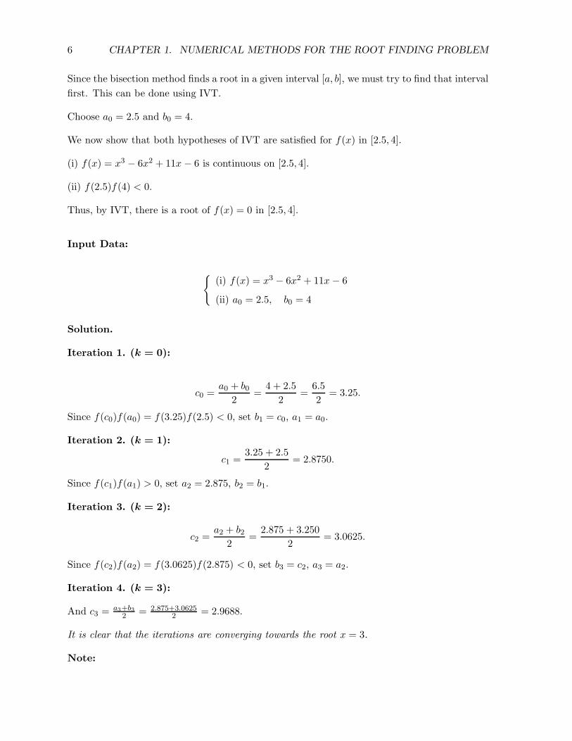
Example 1.3
Find the positive root of f(x) = x3 − 6x2 + 11x− 6 = 0 using Bisection method.
Solution:
Finding the interval [a, b] bracketing the root:
6 CHAPTER 1. NUMERICAL METHODS FOR THE ROOT FINDING PROBLEM
Since the bisection method finds a root in a given interval [a, b], we must try to find that interval
first. This can be done using IVT.
Choose a0 = 2.5 and b0 = 4.
We now show that both hypotheses of IVT are satisfied for f(x) in [2.5, 4].
(i) f(x) = x3 − 6x2 + 11x− 6 is continuous on [2.5, 4].
(ii) f(2.5)f(4) < 0.
Thus, by IVT, there is a root of f(x) = 0 in [2.5, 4].
Input Data:
{
(i) f(x) = x3 − 6x2 + 11x− 6
(ii) a0 = 2.5, b0 = 4
Solution.
Iteration 1. (k = 0):
c0 =a0 + b0
2=
4 + 2.5
2=
6.5
2= 3.25.
Since f(c0)f(a0) = f(3.25)f(2.5) < 0, set b1 = c0, a1 = a0.
Iteration 2. (k = 1):
c1 =3.25 + 2.5
2= 2.8750.
Since f(c1)f(a1) > 0, set a2 = 2.875, b2 = b1.
Iteration 3. (k = 2):
c2 =a2 + b2
2=
2.875 + 3.250
2= 3.0625.
Since f(c2)f(a2) = f(3.0625)f(2.875) < 0, set b3 = c2, a3 = a2.
Iteration 4. (k = 3):
And c3 = a3+b32 = 2.875+3.0625
2 = 2.9688.
It is clear that the iterations are converging towards the root x = 3.
Note:
1.3. BISECTION-METHOD 7
1. From the statement of the bisection algorithm, it is clear that the algorithm always con-
verges.
2. The example above shows that the convergence, however, can be very slow.
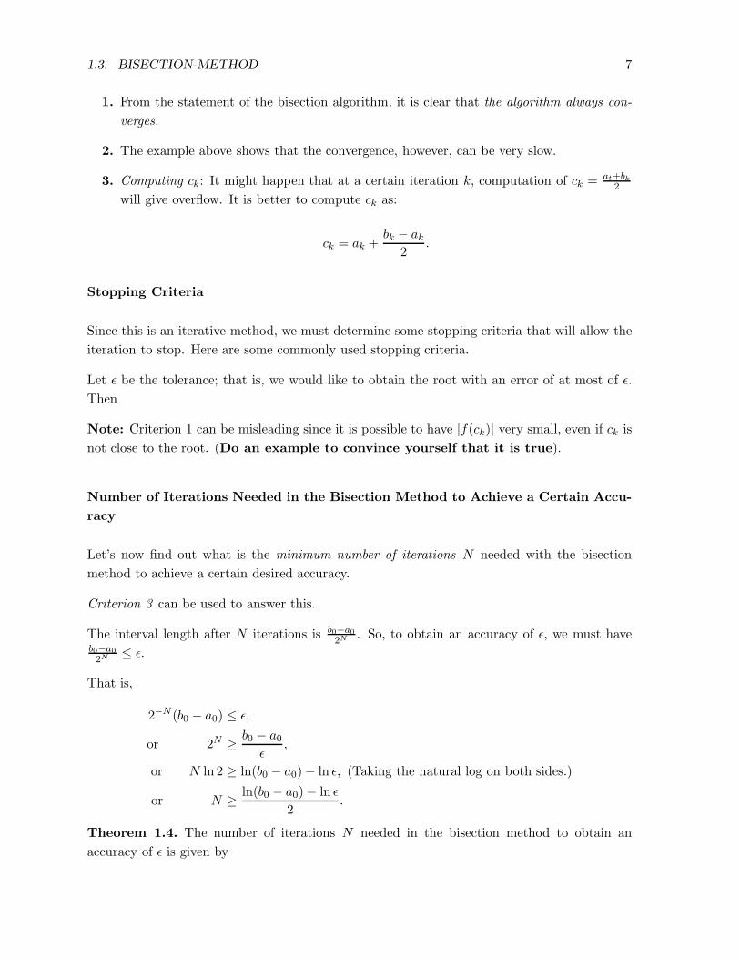
3. Computing ck: It might happen that at a certain iteration k, computation of ck = at+bk2
will give overflow. It is better to compute ck as:
ck = ak +bk − ak
2.
Stopping Criteria
Since this is an iterative method, we must determine some stopping criteria that will allow the
iteration to stop. Here are some commonly used stopping criteria.
Let ǫ be the tolerance; that is, we would like to obtain the root with an error of at most of ǫ.
Then
Note: Criterion 1 can be misleading since it is possible to have |f(ck)| very small, even if ck is
not close to the root. (Do an example to convince yourself that it is true).
Number of Iterations Needed in the Bisection Method to Achieve a Certain Accu-
racy
Let’s now find out what is the minimum number of iterations N needed with the bisection
method to achieve a certain desired accuracy.
Criterion 3 can be used to answer this.
The interval length after N iterations is b0−a02N
. So, to obtain an accuracy of ǫ, we must haveb0−a02N
≤ ǫ.
That is,
2−N (b0 − a0) ≤ ǫ,
or 2N ≥ b0 − a0ǫ
,
or N ln 2 ≥ ln(b0 − a0)− ln ǫ, (Taking the natural log on both sides.)
or N ≥ ln(b0 − a0)− ln ǫ
2.
Theorem 1.4. The number of iterations N needed in the bisection method to obtain an
accuracy of ǫ is given by
8 CHAPTER 1. NUMERICAL METHODS FOR THE ROOT FINDING PROBLEM
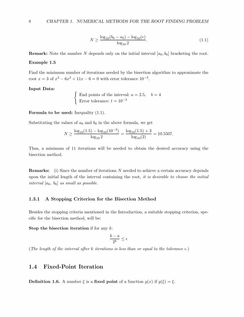
N ≥ log10(b0 − a0)− log10(ǫ)
log10 2. (1.1)
Remark: Note the number N depends only on the initial interval [a0, b0] bracketing the root.
Example 1.5
Find the minimum number of iterations needed by the bisection algorithm to approximate the
root x = 3 of x3 − 6x2 + 11x− 6 = 0 with error tolerance 10−3.
Input Data:{
End points of the interval: a = 2.5, b = 4
Error tolerance: t = 10−3
Formula to be used: Inequality (1.1).
Substituting the values of a0 and b0 in the above formula, we get
N ≥ log10(1.5) − log10(10−3)
log10 2=
log10(1.5) + 3
log10(2)= 10.5507.
Thus, a minimum of 11 iterations will be needed to obtain the desired accuracy using the
bisection method.
Remarks: (i) Since the number of iterations N needed to achieve a certain accuracy depends
upon the initial length of the interval containing the root, it is desirable to choose the initial
interval [a0, b0] as small as possible.
1.3.1 A Stopping Criterion for the Bisection Method
Besides the stopping criteria mentioned in the Introduction, a suitable stopping criterion, spe-
cific for the bisection method, will be:
Stop the bisection iteration if for any k:
b− a
2k≤ ǫ
(The length of the interval after k iterations is less than or equal to the tolerance ǫ.)
1.4 Fixed-Point Iteration
Definition 1.6. A number ξ is a fixed point of a function g(x) if g(ξ) = ξ.

1.4. FIXED-POINT ITERATION 9
Suppose that the equation f(x) = 0 is written in the form x = g(x); that is,
f(x) = x− g(x) = 0.
Then any fixed point ξ of g(x) is a root of f(x) = 0 because
f(ξ) = ξ − g(ξ) = ξ − ξ = 0.
Thus, a root of f(x) = 0 can be found by finding a fixed point of x = g(x), which corresponds
to f(x) = 0.
Finding a root of f(x) = 0 by finding a fixed point of x = g(x) immediately suggests an iterative
procedure of the following type.
Start with an initial guess x0 of the root and form a sequence {xk} defined by
xk+1 = g(xk), k = 0, 1, 2, . . .
If the sequence {xk} converges, then limk→∞
xk = ξ will be a root of f(x) = 0.
The question therefore rises:
Given f(x) = 0 in [a, b].
How do we write f(x) = 0 in the form x = g(x) such that the sequence {xk} is defined by
xk+1 = g(xk);
will converge to the root x = ξ for any choice of the initial approximation x0?
The simplest way to write f(x) = 0 in the form x = g(x) is to add x on both sides, that is,
x = f(x) + x = g(x).
But it does not very often work.
To convince yourself, consider Example 1.3 again. Here,
f(x) = x3 − 6x2 + 11x− 6 = 0.
Define
g(x) = x+ f(x) = x3 − 6x2 + 12x− 6.
We know that there is a root of f(x) in [2.5, 4]; namely x = 3.

10 CHAPTER 1. NUMERICAL METHODS FOR THE ROOT FINDING PROBLEM
Let’s start the iteration xk+1 = g(xk) with x0 = 3.5.
Then we have:
x1 = g(x0) = g(3.5) = 5.3750,
x2 = g(x1) = g(5.3750) = 40.4434,
x3 = g(x2) = g(40.4434) = 5.6817 × 10⁴,
and x4 = g(x3) = g(5.6817 × 10⁴) = 1.8340 × 10¹⁴.
The sequence {xk} is clearly diverging.
The convergence and divergence of the fixed-point iteration are illustrated by the following
graphs.
Figure 1.2: Convergence of the Fixed-Point Iteration
Fixed-Point
y=x
x2 x1 x0
A Sufficient Condition for Convergence
The following theorem gives a sufficient condition on g(x) which ensures the convergence of the
sequence {xk} with any initial approximation x0 in [a, b].
Theorem 1.7 (Fixed-Point Iteration Theorem). Let f(x) = 0 be written in the form
x = g(x). Assume that g(x) satisfies the following properties:
(i) For all x in [a, b], g(x) ∈ [a, b]; that is g(x) takes every value between a and b.

1.4. FIXED-POINT ITERATION 11
Figure 1.3: Divergence of the Fixed-Point Iteration
Fixed-Point
y=x
x2x1x0
(ii) g′(x) exists on (a, b) with the property that there exists a positive constant 0 < r < 1
such that
|g′(x)| ≤ r,
for all x in (a, b).
Then
(i) there is a unique fixed point x = ξ of g(x) in [a, b],
(ii) for any x0 in [a, b], the sequence {xk} defined by
xk+1 = g(xk), k = 0, 1, · · ·
converges to the fixed point x = ξ; that is, to the root ξ of f(x) = 0.
The proof of the fixed-point theorem will require two important theorems from calculus: Initial
Value Theorem (IVT) and the Mean Value Theorem (MVT). The IVT has been stated
earlier. We will now state the MVT.
The Mean Value Theorem (MVT)
Let f(x) be a function such that
(i) it is continuous on [a, b]
12 CHAPTER 1. NUMERICAL METHODS FOR THE ROOT FINDING PROBLEM
(ii) it is differentiable on (a, b)
Then there is a number c in (a, b) such that
f(b)− f(a)
b− a= f ′(c)
Proof of the Fixed-Point Theorem:
The proof comes in three parts: Existence, Uniqueness, and Convergence.
Since a fixed point of g(x) is a root of f(x) = 0, this amounts to proving that there is a fixed
point in [a, b] and it is unique.
Proof of Existence
First, consider the case where either g(a) = a or g(b) = b.
• If g(a) = a, then x = a is a fixed point of g(x). Thus, x = a is a root of f(x) = 0.
• If g(b) = b, then x = b is a fixed point of g(x). Thus x = b is a root of f(x) = 0.
Next, consider the general case where the above assumptions are not true. That is, g(a) 6= a
and g(b) 6= b.
In such a case, g(a) > a and g(b) < b. This is because, by Assumption 1, both g(a) and g(b)
are in [a, b], and since g(a) 6= a and g(b) 6= b, g(a) must be greater than a and g(b) must be
greater than b.
Now, define the function h(x) = g(x) − x. We will now show that h(x) satisfies both the
hypotheses of the Intermediate Value Theorem (IVT).
In this context, we note
(i) since g(x) is continuous by our assumptions, h(x) is also continuous on [a, b]. (Hypothesis
(i) is satisfied)
(ii) h(a) = g(a)− a > 0 and h(b) = g(b) − b < 0. (Hypothesis (ii) is satisfied)

1.4. FIXED-POINT ITERATION 13
Since both hypotheses of the IVT are satisfied, by this theorem, there exists a number c in [a, b]
such that
h(c) = 0
this means g(c) = c.
That is, x = c is a fixed point of g(x). This proves the Existence part of the Theorem.
Proof of Uniqueness (by contradiction):
We will prove the uniqueness by contradiction. Our line of proof will be as follows:
We will first assume that there are two fixed points of g(x) in [a, b] and then show that this
assumption leads to a contradiction.
Suppose ξ1 and ξ2 are two fixed points in [a, b], and ξ1 6= ξ2.
The proof is based on the Mean Value Theorem applied to g(x) in [ξ1, ξ2].
In this context, note that g(x) is differentiable and hence, continuous on [ξ1, ξ2].
So, by MVT, we can find a number c in (ξ1, ξ2) such that
g(ξ2)− g(ξ1)
(ξ2 − ξ1)= g′(c).
Since g(ξ1) = ξ1, and g(ξ2) = ξ2, (because they are fixed points of g(x)), we get
ξ2 − ξ1ξ2 − ξ1
= g′(c).
That is, g′(c) = 1, which is a contradiction to our Assumption 2. Thus, ξ1 can not be different
from ξ2, this proves the uniqueness.
Proof of Convergence:
Let ξ be the root of f(x) = 0. Then the absolute error at step k + 1 is given by
ek+1 = |ξ − xk+1|. (1.2)
To prove that the sequence converges, we need to show that limk→∞ ek+1 = 0.
14 CHAPTER 1. NUMERICAL METHODS FOR THE ROOT FINDING PROBLEM
To show this, we apply the Mean Value Theorem to g(x) in [xk, ξ]. Since g(x) also satisfies
both the hypotheses of the MVT in [xk, ξ], we get
g(ξ) − g(xk)
ξ − xk= g′(c) (1.3)
where xk < c < ξ.
Now, x = ξ is a fixed point of g(x), so we have (by definition):
(i) g(ξ) = ξ.
Also, from the iteration x = g(x), we have
(ii) xk+1 = g(xk).
So, from ( ), we getξ − xk+1
ξ − xk= g′(c)
Taking absolute values on both sides we have
|ξ − xk+1||ξ − xk|
= |g′(c)| (1.4)
orek+1
ek= |g′(c)|. (1.5)
Since |g′(c)| ≤ r, we have ek+1 ≤ rek.
Since the above relation ( ) is true for every k, we have ek ≤ rek−1. Thus, ek+1 ≤ r2ek−1.
Continuing in this way, we finally have ek+1 ≤ rk+1e0, where e0 is the initial error. (That is,
e0 = |x0 − ξ|).
Since r < 1, we have rk+1 → 0 as k → ∞.
Thus,
limk→∞
ek+1 = limk→∞
|xk+1 − ξ|
≤ limk→∞
rk+1e0 = 0
This proves that the sequence {xk} converges to x = ξ and that x = ξ is the only fixed point
of g(x).

1.4. FIXED-POINT ITERATION 15
In practice, it is not easy to verify Assumption 1. The following corollary of the fixed-point
theorem is more useful in practice because the conditions here are more easily verifiable. We
leave the proof of the corollary as an [Exercise].
Corollary 1.8. Let the iteration function g(x) be such that
(i) it is continuously differentiable in some open interval containing the fixed point x = ξ,
(ii) |g′(ξ)| < 1.
Then there exists a number ǫ > 0 such that the iteration: xk+1 = g(xk) converges whenever x0
is chosen in |x0 − ξ| ≤ ǫ.
Example 1.9
Find a positive zero of x3 − 6x2 + 11x− 6 in [2.5, 4] using fixed-point iterations.
Input Data:{
(i) f(x) = x3 − 6x2 + 11x− 6,
(ii) a = 2.5, b = 4.
Solution.
Step 1. Writing f(x) = 0 in the form x = g(x) so that both hypotheses of Theorem 1.7 are
satisfied.
We have seen in the last section that the obvious form: g(x) = x+ f(x) = x3 − 6x2 + 12x− 6
does not work.
Let’s now write f(x) = 0 in the form: x = 111(−x3 + 6x2 + 6) = g(x).
Then (i) for all x ∈ [2.5, 4], g(x) ∈ [2.5, 4] (Note that g(2.5) = 2.5341 and g(4) = 3.4545).
(ii) g′(x) = 111 (−3x2 + 12x) steadily decreases in [2.5, 4] and remains less than 1 for all x in
(2.5, 4). (Note that g′(2.5) = 1.0227 and g′(4) = 0.)
Thus, both hypotheses of Theorem 1.6 are satisfied. So, according to this theorem, for any x0
in [2.5, 4], the sequence {xk} should converge to the fixed point.
We now do a few iterations to verify this assertion. Starting with x0 = 3.5 and using the
iteration:
xk+1 = g(xk) = − 111(3x
2k + 12xk)
(k = 0, 1, 2, . . . , 11)
We obtain:
16 CHAPTER 1. NUMERICAL METHODS FOR THE ROOT FINDING PROBLEM
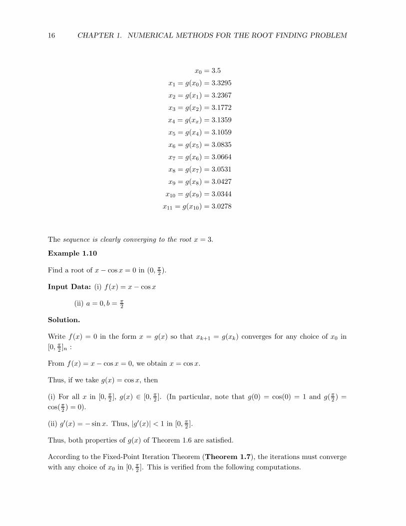
x0 = 3.5
x1 = g(x0) = 3.3295
x2 = g(x1) = 3.2367
x3 = g(x2) = 3.1772
x4 = g(xx) = 3.1359
x5 = g(x4) = 3.1059
x6 = g(x5) = 3.0835
x7 = g(x6) = 3.0664
x8 = g(x7) = 3.0531
x9 = g(x8) = 3.0427
x10 = g(x9) = 3.0344
x11 = g(x10) = 3.0278
The sequence is clearly converging to the root x = 3.
Example 1.10
Find a root of x− cos x = 0 in (0, π2 ).
Input Data: (i) f(x) = x− cos x
(ii) a = 0, b = π2
Solution.
Write f(x) = 0 in the form x = g(x) so that xk+1 = g(xk) converges for any choice of x0 in
[0, π2 ]n :
From f(x) = x− cos x = 0, we obtain x = cos x.
Thus, if we take g(x) = cos x, then
(i) For all x in [0, π2 ], g(x) ∈ [0, π2 ]. (In particular, note that g(0) = cos(0) = 1 and g(π2 ) =
cos(π2 ) = 0).
(ii) g′(x) = − sinx. Thus, |g′(x)| < 1 in [0, π2 ].
Thus, both properties of g(x) of Theorem 1.6 are satisfied.
According to the Fixed-Point Iteration Theorem (Theorem 1.7), the iterations must converge
with any choice of x0 in [0, π2 ]. This is verified from the following computations.

1.5. THE NEWTON METHOD 17
x0 = 0
x1 = cosxo = 1
x2 = cosx1 = 0.5403
x3 = cosx2 = 0.8576
...
x17 = 0.73956
x18 = cosx17 = 0.73955
1.5 The Newton Method
The Newton- method, described below, shows that there is a special choice of g(x) that will
allow us to readily use the results of Corollary 1.8.
Assume that f ′′(x) exists and is continuous on [a, b] and ξ is a simple root of f(x), that is,
f(ξ) = 0 and f ′(ξ) 6= 0.
Choose
g(x) = x− f(x)
f ′(x).
Then g′(x) = 1− (f ′(x))2−f(x)f ′′(x)(f ′(x))2 = f(x)f ′′(x)
(f ′(x))2 .
Thus, g′(ξ) = f(ξ)f ′′(ξ)(f ′(ξ))2
= 0, since f(ξ) = 0, and f ′(ξ) 6= 0.
Since g′(x) is continuous, this means that there exists a small neighborhood around the root
x = ξ such that for all points x in that neighborhood, |g′(x)| < 1.
Thus, if g(x) is chosen as above and the starting approximation x0 is chosen sufficiently close
to the root x = ξ, then the fixed-point iteration is guaranteed to converge.
This leads us to the following well-known classical method known as the Newton method.
Note: In many text books and literature, Newton’s Method is referred to as Newton’s
Method. See the article about this in SIAM Review (1996).
Algorithm 1.11 (The Newton Method).
Inputs: f(x) - The given function
x0 - The initial approximation
ǫ - The error tolerance
N - The maximum number of iterations

18 CHAPTER 1. NUMERICAL METHODS FOR THE ROOT FINDING PROBLEM
Output: An approximation to the root x = ξ or a message of failure.
Assumption: x = ξ is a simple root of f(x).
For k = 0, 1, · · · , do until convergence or failure.
• Compute f(xk), f′(xk).
• Compute xk+1 = xk −f(xk)
f ′(xk).
• Test for convergence or failure:
If |f(xk)| < ǫ,
or|xk+1 − xk|
|xk|< ǫ,
or k > N, stop.
stopping criteria.
End
Definition 1.12. The iterations xk+1 = xk − f(xk)f ′(xk)
are called Newton’s iterations.
Example 1.13
Find a positive real root of cos x− x3 = 0.
Obtaining an initial approximation: Since cos x ≤ 1 for all x and for x > 1, x3 > 1, the
positive zero must lie between 0 and 1. So, let’s take x0 = 0.5.
Input Data:
(i) The function f(x) = cos x− x3
(ii) Initial approximation: x0 = 0.5
Formula to be used: xk+1 = xk − f(xk)f ′(xk)
Solution.
Compute f ′(x) = − sinx− 3x2.
Iteration 1. k=0: x1 = x0 − f(x0)f ′(x0)
= 0.5− cos(0.5)−(0.5)3
− sin(0.5)−3(0.5)2= 1.1121.
Iteration 2. k=1: x2 = x1 − f(x1
f ′(x1)= 0.9097.
Iteration 3. k=2: x3 = x2 − f(x2)f ′(x2)
= 0.8672.
Iteration 4. k=3: x4 = x3 − f(x3)f ′(x3)
= 0.8654.
1.5. THE NEWTON METHOD 19
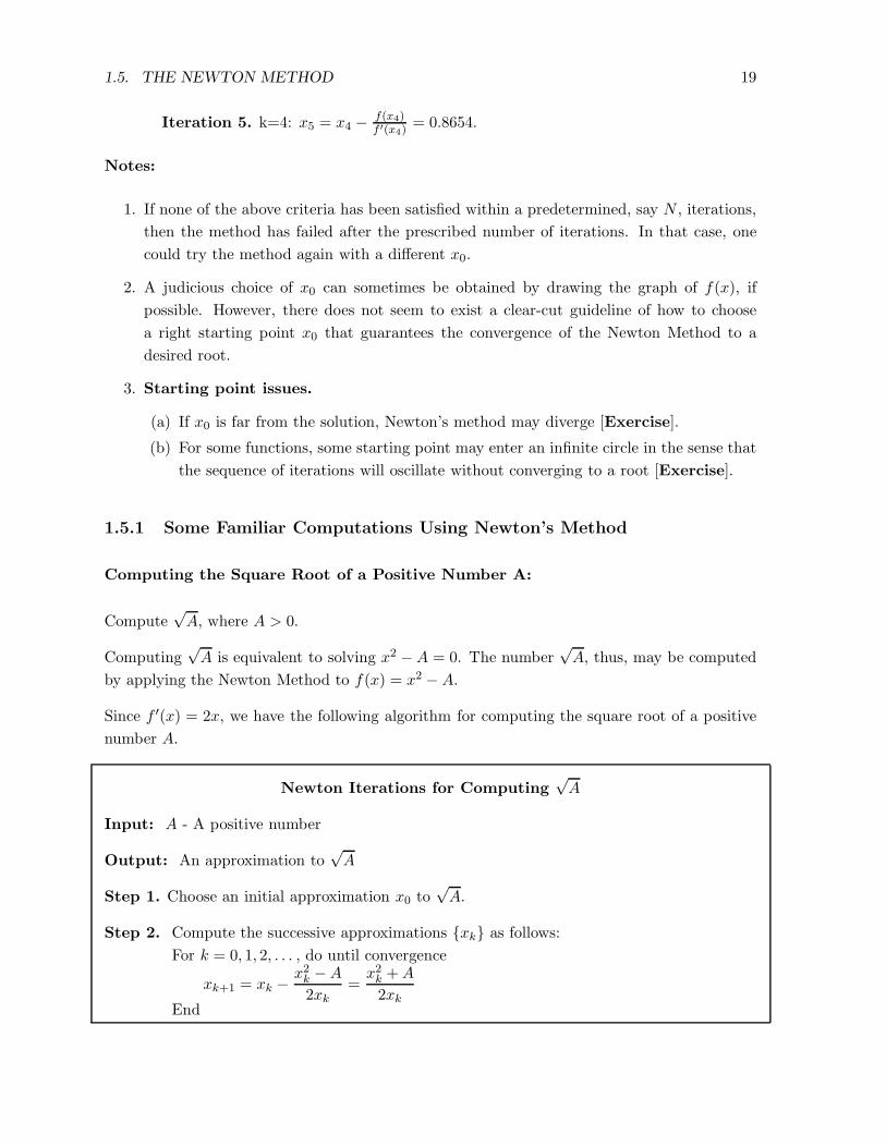
Iteration 5. k=4: x5 = x4 − f(x4)f ′(x4)
= 0.8654.
Notes:
1. If none of the above criteria has been satisfied within a predetermined, say N , iterations,
then the method has failed after the prescribed number of iterations. In that case, one
could try the method again with a different x0.
2. A judicious choice of x0 can sometimes be obtained by drawing the graph of f(x), if
possible. However, there does not seem to exist a clear-cut guideline of how to choose
a right starting point x0 that guarantees the convergence of the Newton Method to a
desired root.
3. Starting point issues.
(a) If x0 is far from the solution, Newton’s method may diverge [Exercise].
(b) For some functions, some starting point may enter an infinite circle in the sense that
the sequence of iterations will oscillate without converging to a root [Exercise].
1.5.1 Some Familiar Computations Using Newton’s Method
Computing the Square Root of a Positive Number A:
Compute√A, where A > 0.
Computing√A is equivalent to solving x2 −A = 0. The number
√A, thus, may be computed
by applying the Newton Method to f(x) = x2 −A.
Since f ′(x) = 2x, we have the following algorithm for computing the square root of a positive
number A.
Newton Iterations for Computing√A
Input: A - A positive number
Output: An approximation to√A
Step 1. Choose an initial approximation x0 to√A.
Step 2. Compute the successive approximations {xk} as follows:
For k = 0, 1, 2, . . . , do until convergence
xk+1 = xk −x2k −A
2xk=
x2k +A
2xkEnd
20 CHAPTER 1. NUMERICAL METHODS FOR THE ROOT FINDING PROBLEM
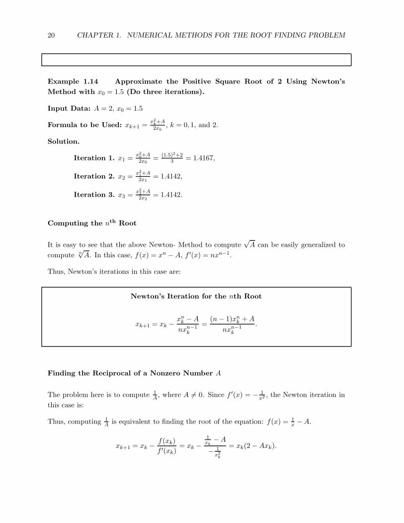
Example 1.14 Approximate the Positive Square Root of 2 Using Newton’s
Method with x0 = 1.5 (Do three iterations).
Input Data: A = 2, x0 = 1.5
Formula to be Used: xk+1 =x2k+A
2xk
, k = 0, 1, and 2.
Solution.
Iteration 1. x1 =x20+A
2x0= (1.5)2+2
3 = 1.4167,
Iteration 2. x2 =x21+A
2x1= 1.4142,
Iteration 3. x3 =x22+A
2x2= 1.4142.
Computing the nth Root
It is easy to see that the above Newton- Method to compute√A can be easily generalized to
compute n√A. In this case, f(x) = xn −A, f ′(x) = nxn−1.
Thus, Newton’s iterations in this case are:
Newton’s Iteration for the nth Root
xk+1 = xk −xnk −A
nxn−1k
=(n− 1)xnk +A
nxn−1k
.
Finding the Reciprocal of a Nonzero Number A
The problem here is to compute 1A, where A 6= 0. Since f ′(x) = − 1
x2 , the Newton iteration in
this case is:
Thus, computing 1A
is equivalent to finding the root of the equation: f(x) = 1x−A.
xk+1 = xk −f(xk)
f ′(xk)= xk −
1xk
−A
− 1x2k
= xk(2−Axk).
1.5. THE NEWTON METHOD 21
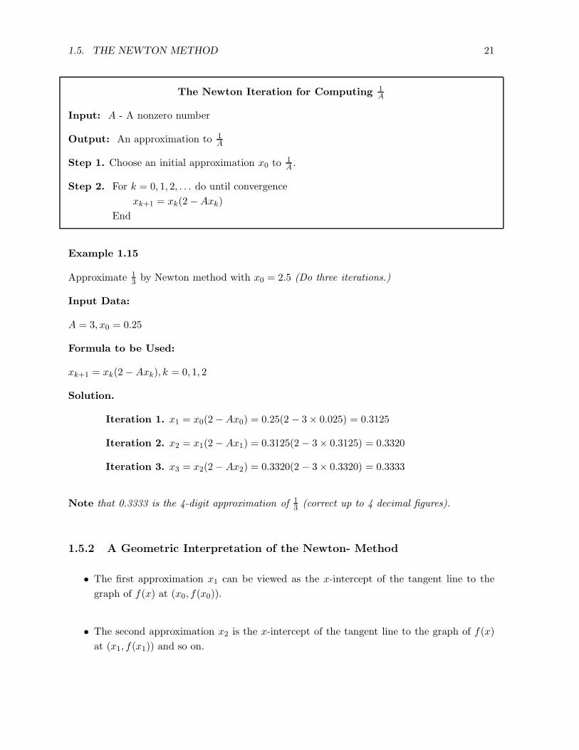
The Newton Iteration for Computing 1A
Input: A - A nonzero number
Output: An approximation to 1A
Step 1. Choose an initial approximation x0 to 1A.
Step 2. For k = 0, 1, 2, . . . do until convergence
xk+1 = xk(2−Axk)
End
Example 1.15
Approximate 13 by Newton method with x0 = 2.5 (Do three iterations.)
Input Data:
A = 3, x0 = 0.25
Formula to be Used:
xk+1 = xk(2−Axk), k = 0, 1, 2
Solution.
Iteration 1. x1 = x0(2−Ax0) = 0.25(2 − 3× 0.025) = 0.3125
Iteration 2. x2 = x1(2−Ax1) = 0.3125(2 − 3× 0.3125) = 0.3320
Iteration 3. x3 = x2(2−Ax2) = 0.3320(2 − 3× 0.3320) = 0.3333
Note that 0.3333 is the 4-digit approximation of 13 (correct up to 4 decimal figures).
1.5.2 A Geometric Interpretation of the Newton- Method
• The first approximation x1 can be viewed as the x-intercept of the tangent line to the
graph of f(x) at (x0, f(x0)).
• The second approximation x2 is the x-intercept of the tangent line to the graph of f(x)
at (x1, f(x1)) and so on.

22 CHAPTER 1. NUMERICAL METHODS FOR THE ROOT FINDING PROBLEM
Figure 1.4: Graphical Representation of the Newton Method.
x0x2
x1
f(x0)
f(x1)
ξ
tangent to f(x0)
tangent to f(x1)
1.5.3 The Secant Method
A major disadvantage of the Newton Method is the requirement of finding the value of the deriva-
tive of f(x) at each approximation. There are functions for which this job is either extremely
difficult (if not impossible) or time consuming. A way out is to approximate the derivative by
knowing the values of the function at that and the previous approximation. Knowing f(xk)
and f(xk−1), we can approximate f ′(xk) as:
f ′(xk) ≈f(xk)− f(xk−1)
xk − xk−1.
Then, the Newton iterations in this case become:
xk+1 = xk −f(xk)
f ′(xk)
≈ xk −f(xk)(xk − xk−1)
f(xk)− f(xk−1).

1.5. THE NEWTON METHOD 23
This consideration leads to the Secant method.
Algorithm 1.16 (The Secant Method).
Inputs: f(x) - The given function
x0, x1 - The two initial approximations of the root
ǫ - The error tolerance
N - The maximum number of iterations
Output: An approximation of the exact solution ξ or a message of failure.
For k = 1, 2, · · · , until the stopping criteria is met,
• Compute f(xk) and f(xk−1).
• Compute the next approximation: xk+1 = xk − f(xk)(xk−xk−1)f(xk)−f(xk−1)
.
• Test for convergence or maximum number of iterations: If |xk+1 − xk| < ǫ or if k > N ,
Stop.
End
Note: The secant method needs two approximations x0 and x1 to start with, whereas the
Newton method just needs one, namely, x0.
Example 1.17
Approximate the Positive Square Root of 2, choosing x0 = 1.5 and x1 = 1 (Do four iterations).
Input Data:
The function f(x) = x2 − 2
Initial approximations: x0 = 1.5, x1 = 1
Formula to be Used: xk+1 = xc − f(xk)(xk−xk−1)f(xk)−f(xk−1)
Solution.
Iteration 1. (k = 1). Compute x2 from x0 and x1:
x2 = x1 −f(x1)(x1 − x0)
f(x1)− f(x0)
= 1− (−1)(−.5)
−1− .25= 1 +
.5
1.25= 1.4,

24 CHAPTER 1. NUMERICAL METHODS FOR THE ROOT FINDING PROBLEM
Iteration 2. (k = 2). Compute x3 from x1 and x2:
x3 = x2 −f(x2)(x2 − x1)
f(x2)− f(x1)
= 1.4 − (−0.04)(0.4)
(−0.04) − (−1)
= 1.4 + 0.0167
= 1.4167,
Iteration 3. (k = 3). Compute x4 from x2 and x3:
x4 = x3 −f(x3)(x3 − x2)
f(x3)− f(x2)
= 1.4142,
Iteration 4. (k = 4). Compute x5 from x3 and x4:
and
x5 = x4 −f(x4)(x4 − x3)
f(x4)− f(x3)= 1.4142.
Note: By comparing the results of this example with those obtained by the Newton method
Example 1.14, we see that
it took 4 iterations by the secant method to obtain a 4-digit accuracy of√2 = 1.4142; whereas
for the Newton method, this accuracy was obtained just after 2 iterations.
In general, the Newton method converges faster than the secant method. The exact rate of
convergence of these two and the other methods will be discussed in the next section.
1.5.4 A Geometric Interpretation of the Secant Method
• x2 is the x-intercept of the secant line passing through (x0, f(x0)) and (x1, f(x1)).
• x3 is the x-intercept of the secant-line passing through (x1, f(x1)) and (x2, f(x2)).
• And so on.
Note: That is why the method is called the secant method.
1.6 The Method of False Position (The Regular Falsi Method)
In the Bisection method, every interval under consideration is guaranteed to have the desired
root x = ξ. That is why the Bisection method is often called a bracket method, because every

1.6. THE METHOD OF FALSE POSITION (THE REGULAR FALSI METHOD) 25
Figure 1.5: Geometric Interpretation of the Secant Method
(x1, f(x1))
x2
x1x = ξx0
(x0, f(x0))
(x2, f(x2))
interval brackets the root. However, the Newton method and the secant method are not bracket
methods in that sense, because there is no guarantee that the two successive approximations
will bracket the root. Here is an example.
Example 1.18
(The Secant Method does not bracket the root.)
Compute a zero of tan(πx)−6 = 0, choosing x0 = 0, and x1 = 0.48, using the Secant Method.
(Note that ξ = 0.44743154 is a root of f(x) = 0 lying in the interval [0, 0.48]).
Iteration 1. (k = 1). Compute x2:
x2 = x1 − f(x1)(x1−x0)
f(x1)−f(x0)= 0.181194.
Iteration 2. (k = 2). Compute x3:
x1 = 0.48, x2 = 0.181194. (Two starting initial approximations for Iteration 2.)
x3 = x2 − f(x2)(x2−x1)
f(x2)−f(x1)= 0.286187
Iteration 3. (k = 3). Compute x4: x2 = 0.181194, x3 = 0.286187. (Two starting initial
approximations for Iteration 3.)
x4 = x3 − f(x3)(x3−x2)
f(x3)−f(x2)= 1.091987.
Clearly, the iterations are diverging, despite of the fact of the initial interval [0, 0.48]
26 CHAPTER 1. NUMERICAL METHODS FOR THE ROOT FINDING PROBLEM
brackets the root.
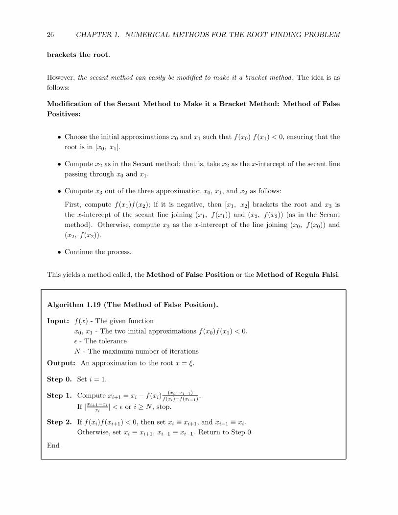
However, the secant method can easily be modified to make it a bracket method. The idea is as
follows:
Modification of the Secant Method to Make it a Bracket Method: Method of False
Positives:
• Choose the initial approximations x0 and x1 such that f(x0) f(x1) < 0, ensuring that the
root is in [x0, x1].
• Compute x2 as in the Secant method; that is, take x2 as the x-intercept of the secant line
passing through x0 and x1.
• Compute x3 out of the three approximation x0, x1, and x2 as follows:
First, compute f(x1)f(x2); if it is negative, then [x1, x2] brackets the root and x3 is
the x-intercept of the secant line joining (x1, f(x1)) and (x2, f(x2)) (as in the Secant
method). Otherwise, compute x3 as the x-intercept of the line joining (x0, f(x0)) and
(x2, f(x2)).
• Continue the process.
This yields a method called, the Method of False Position or the Method of Regula Falsi.
Algorithm 1.19 (The Method of False Position).
Input: f(x) - The given function
x0, x1 - The two initial approximations f(x0)f(x1) < 0.
ǫ - The tolerance
N - The maximum number of iterations
Output: An approximation to the root x = ξ.
Step 0. Set i = 1.
Step 1. Compute xi+1 = xi − f(xi)(xi−xi−1)
f(xi)−f(xi−1).
If |xi+1−xi
xi| < ǫ or i ≥ N , stop.
Step 2. If f(xi)f(xi+1) < 0, then set xi ≡ xi+1, and xi−1 ≡ xi.
Otherwise, set xi ≡ xi+1, xi−1 ≡ xi−1. Return to Step 0.
End

1.6. THE METHOD OF FALSE POSITION (THE REGULAR FALSI METHOD) 27
Example 1.20
Consider again the previous example: (Example 1.18). Find the positive root of tan(πx)−6 =
0 in [0, 0.48], using the Method of False Position.
Input Data:
f(x) = tan(πx)− 6,
Initial approximation: x0 = 0, x1 = 0.48
Formula to be Used: xi+1 = xi − f(xi)(xi−xi−1)
f(xi)−f(xi−1)
Solution.
Iteration 1. (Initial approximations for Iteration 1: x0 = 0, x1 = 0.48).
Step 1. x2 = x1 − f(x1)x1−x0
f(x1)−f(x0)= 0.181192
Step 2. f(x2)f(x1) < 0
Set x0 = 0.48, x1 = 0.181192.
Iteration 2. (Initial approximations for Iteration 2: x0 = 0.48, x1 = 0.181192).
Step 1. x2 = x1 − f(x1)x1−x0
f(x1)−f(x0)= 0.286186
Step 2. f(x2)f(x1) > 0
Set x0 = 0.48, x1 = 0.286186.
Iteration 3. (Initial approximations for Iteration 3: x0 = 0.48, x1 = 0.286186).
Step 1. x2 = 0.348981
Step 2. f(x2)f(x1) > 0
Set x0 = 0.48, x1 = 0.348981.
Iteration 4. (Initial approximations for Iteration 4: x0 = 0.48, x1 = 0.348981).
Step 1. x2 = 0.387053
Step 2. f(x2)f(x1) > 0
Iteration 5. (Initial approximations for Iteration 5: x0 = 0.48, x1 = 0.387053).
Step 1. x2 = 0.410305
28 CHAPTER 1. NUMERICAL METHODS FOR THE ROOT FINDING PROBLEM
1.7 Convergence Analysis of the Iterative Methods
We have seen that the Bisection method always converges, and each of the methods: the
Newton Method, the Secant method, and the method of False Position, converges under certain
conditions. The question now arises:
When a method converges, how fast does it converge?
In other words, what is the rate of convergence? To this end, we first define:
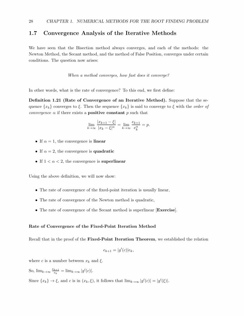
Definition 1.21 (Rate of Convergence of an Iterative Method). Suppose that the se-
quence {xk} converges to ξ. Then the sequence {xk} is said to converge to ξ with the order of
convergence α if there exists a positive constant p such that
limk→∞
|xk+1 − ξ||xk − ξ|α = lim
k→∞ek+1
eαk= p.
• If α = 1, the convergence is linear
• If α = 2, the convergence is quadratic
• If 1 < α < 2, the convergence is superlinear
Using the above definition, we will now show:
• The rate of convergence of the fixed-point iteration is usually linear,
• The rate of convergence of the Newton method is quadratic,
• The rate of convergence of the Secant method is superlinear [Exercise].
Rate of Convergence of the Fixed-Point Iteration Method
Recall that in the proof of the Fixed-Point Iteration Theorem, we established the relation
ek+1 = |g′(c)|ek,
where c is a number between xk and ξ.
So, limk→∞ek+1
ek= limk→∞ |g′(c)|.
Since {xk} → ξ, and c is in (xk, ξ), it follows that limk→∞ |g′(c)| = |g′(ξ)|.

1.7. CONVERGENCE ANALYSIS OF THE ITERATIVE METHODS 29
This gives limk→∞ek+1
ek= |g′(ξ)|. Thus α = 1.
We, therefore, have
The fixed point iteration scheme has linear rate of convergence, when it converges.
Rate of Convergence of the Newton Method
To study the rate of convergence of the Newton Method, we need Taylor’s Theorem.
Taylor’s Theorem of order n
Suppose
(i) f(x) possesses continuous derivatives of order up to n+ 1 in [a, b],
(ii) p is a point in [a, b].
Then for every x in this interval, there exists a number c (depending upon x) between p and x
such that
f(x) = f(p) + f ′(p)(x− p) +f ′(p)2!
(x− p)2 + · · ·+ fn(p)
n!(n− p)n +Rn(x),
where Rn(x), called the remainder after n terms, is given by:
Rn(x) =f (n+1)(c)
(n + 1)!(x− p)n+1.
Let’s choose a small interval around the root x = ξ. Then, for any x in this interval, we have,
by Taylor’s theorem of order 1, the following expansion of the function g(x):
g(x) = g(ξ) + (x− ξ)g′(ξ) +(x− ξ)2
2!g′′(ηk)
where ηk lies between x and ξ.
Now, for the Newton Method, we have seen that g′(ξ) = 0.

30 CHAPTER 1. NUMERICAL METHODS FOR THE ROOT FINDING PROBLEM
So, setting g′(ξ) = 0 in the above expression, we have
g(x) = g(ξ) +(x− ξ)2
2!g′′(ηk),
or g(xk) = g(ξ) +(xk − ξ)2
2!g′′(ηk),
or g(xk)− g(ξ) =(xk − ξ)2
2!g′′(ηk).
Since g(xk) = xk+1, and g(ξ) = ξ, from the last equation, we have
xk+1 − ξ =(xk − ξ)2
2!g′′(ηk).
Or, ek+1 =e2k
2! ‖g′(ηk)‖. Taking the limit on both sides, limk→0
ek+1
e2k=
1
2‖g′′
(ηk)‖.
That is, |xk+1 − ξ| = |xk−ξ|22 |g′′(ηk)|.
Since ηk lies between x and ξ for every k, it follows that
limk→∞
ηk = ξ.
So, we have limk→∞ek+1
e2k
= lim |g′′(ηk)|2 = |g′′(ξ)|
2 .
Convergence of Newton’s Method for a Single Root
• Newton’s Method has quadratic rate of convergence.
• The quadratic convergence roughly means that the accuracy gets doubled at each iteration.
Convergence of the Newton Method for a Multiple Root
The above proof depends on the assumption f ′(ξ) = 0; that is, f(x) has a simple root at x = ξ.
In case f(x) = 0 has a multiple root, the convergence is no longer quadratic.
It can be shown [Exercise] that the Newton method still converges, but the rate of convergence
is linear rather than quadratic. For example, given the multiplicity is 2, the error decreases by
a factor of approximately 12 with each iteration.

1.8. A MODIFIED NEWTON METHOD FOR MULTIPLE ROOTS 31
The Rate of Convergence for the Secant Method
It can be shown that if the Secant method converges, then the convergence factor α is approxi-
mately 1.6 for sufficiently large k [Exercise].
This is said as “The rate of convergence of the Secant method is superlinear”.
1.8 A Modified Newton Method for Multiple Roots
Recall that the most important underlying assumption in the proof of quadratic convergence of
the Newton method was that f ′(x) is not zero at the approximation x = xk, and in particular
f ′(ξ) 6= 0. This means that ξ is a simple root of f(x) = 0.
The question, therefore, is: How can the Newton method be modified for a multiple root so that
the quadratic convergence can be retained?
Note that if f(x) has a root ξ of multiplicity m, then
f(ξ) = f ′(ξ) = f ′′(ξ) = · · · = f (m−1)(ξ) = 0,
where f (m−1)(ξ) denotes the (m− 1)th derivative of f(x) at x = ξ.
In this case f(x) can be written as
f(x) = (x− ξ)mh(x),
where h(x) is a polynomial of degree at most m− 2.
In case f(x) has a root of multiplicity m, it was suggested by Ralston and Robinowitz (1978)
that, the following modified iteration will ensure quadratic convergence in the Newton method,
under certain conditions [Exercise].
The Newton Iterations for Multiple Roots of Multiplicity m: Method I
xi+1 = xi −mf(xi)
f ′(xi)
Since in practice, the multiplicity m is not known a priori, another useful modification is to
apply the Newton iteration to the function:
u(x) =f(x)
f ′(x)

32 CHAPTER 1. NUMERICAL METHODS FOR THE ROOT FINDING PROBLEM
in place of f(x).
Thus, in this case, the modified Newton iteration becomes xi+1 = xi − u(xi)u′(xi)
.
Note that, since f(x) = (x− ξ)m h(x), u′(x) 6= 0 at x = ξ.
Since u′(xi) =f ′(x)f ′(x)−f(x)f ′′(x)
[f ′(x)]2we have
The Newton Iterations for Multiple Roots: Method II
xi+1 = xi −f(xi)f
′(xi)[f ′(xi)]2 − [f(xi)]f ′′(xi)
Example 1.22
Approximate the double root x = 0 of ex − x− 1 = 0, choosing x0 = 0.5. (Do two iterations.)
Figure 1.6: The Graph of f(x) = ex − x− 1.
Method I
Input Data:
(i) f(x) = ex − x− 1
(ii) Multiplicity of the roots: m = 2
(iii) Initial approximation: x0 = 0.5
Formula to be Used: xi+1 = xi − 2f(xi)f ′(xi)
Solution.
Iteration 1. (i = 0). Compute x1:
x1 = 0.5− 2(e0.5 − 0.5 − 1)
(e0.5 − 1)= .0415 = 4.15 × 10⁻²
1.9. THE NEWTON METHOD FOR POLYNOMIALS 33
Iteration 2. (i = 1). Compute x2:
x2 = 0.0415 − 2(e0.0415 − 0.0415 − 1)
e0.0415 − 1= .00028703 = 2.8703 × 10⁻⁴.
Method II
Input Data:
(i) f(x) = ex − x− 1,
(ii) Initial approximation: x0 = 0.5
Formula to be Used: xi+1 = xi − f(xi)f ′(xi)(f ′(xi)2−f(xi)f ′′(xi))
Solution.
Compute the first and second derivatives of f(x): f ′(x) = ex − 1, f′′
(x) = ex.
Iteration 1. (i = 0). Compute x1:
x1 = f(x0)f ′(x0)
(f ′(x0))2f(x0)f′′ (x0)
= (e0.5−0.5−1)×(e0.5−1)(e0.5)2×(e0.5−0.5−1)×e0.5
= 0.0493 = 4.93 × 10⁻²
Iteration 2. (i = 1). Compute x2:
x2 = f(x1)f ′(x1)
(f ′(x1))2f(x1)f′′ (x1)
= (e0.0493−0.0493−1)×(e0.0493−1)(e0.0493)2×(e0.0493−0.0493−1)×e0.0493
= 4.1180 × 10⁻⁴
1.9 The Newton Method for Polynomials
A major requirement of all the methods that we have discussed so far is the evaluation of f(x)
at successive approximations xk. Furthermore, Newton’s method requires evaluation of the
derivatives of f(x) at each iteration.
If f(x) happens to be a polynomial Pn(x) (which is the case in many practical applications),
then there is an extremely simple classical technique, known as Horner’s Method to compute
Pn(x) at x = z.
• The value Pn(z) can be obtained recursively in n-steps from the coefficients of the polyno-
mial Pn(x).
34 CHAPTER 1. NUMERICAL METHODS FOR THE ROOT FINDING PROBLEM
• Furthermore, as a by-product, one can get the value of the derivative of Pn(x) at x = z;
that is P ′n(z). Then, the scheme can be incorporated in the Newton Method to compute
a zero of Pn(x).
(Note that the Newton Method requires evaluation of Pn(x) and its derivative at successive
iterations).
1.9.1 Horner’s Method
Let Pn(x) = a0 + a1x+ a2x2 + · · · + anx
n and let x = z be given.
We need to compute Pn(z) and P ′n(z).
Let’s write Pn(x) as:
Pn(x) = (x− z) Qn−1 (x) + bo,
where Qn−1(x) = bnxn−1 + bn−1 x
n−2 + · · ·+ b2x+ b1.
Thus, Pn(z) = b0.
Let’s see how to compute b0 recursively by knowing the coefficients of Pn(x)
From above, we have
a0 + a1x+ a2x2 + · · ·+ anx
n = (x− z)(bnxn−1 + bn−1 x
n−2 + · · ·+ b1) + bo
Comparing the coefficients of like powers of x from both sides, we obtain
bn = an
bn−1 − bnz = an−1
⇒ bn−1 = an−1 + bnz
...
and so on.
In general, bk − bk+1z = ak
⇒ bk = ak + bk+1z. k = n− 1, n− 2, . . . , 1, 0.
Thus, knowing the coefficients an, an−1, . . . , a1, a0 of Pn(x), the coefficients bn, bn−1, . . . , b1 of
Qn−1(x) can be computed recursively starting with bn = an, as shown above. That is,
bk = ak + bk+1z, k = n− 1, k = 2, . . . , 1, 0.

1.9. THE NEWTON METHOD FOR POLYNOMIALS 35
Again, note that Pn(z) = b0. So, Pn(z) = b0 = a0 + b1 z.
That is, if we know the coefficients of a polynomial, we can compute the value of the polynomial
at a given point out of these coefficients recursively as shown above.
Algorithm 1.23 (Evaluating Polynomial: Pn(x) = a0+a1xp+a2x2+ . . .+anx
n at x = z).
Input: (i) a0, a1, ..., an - The coefficients of the polynomial Pn(x).
(ii) z - The number at which Pn(x) has to be evaluated.
Output: b0 = Pn(z).
Step 1. Set bn = an.
Step 2. For k = n− 1, n− 2, . . . , 1, 0 do.
Compute bk = ak + bk+1z
Step 3. Set Pn(z) = b0
End
It is interesting to note that as a by-product of above, we also obtain P ′n(z), as the following
computations show.
Computing P ′n(z)
Pn(x) = (x− z)Qn−1(x) + b0
Thus, P ′n(x) = Qn−1(x) + (x− z)Q′
n−1(x).
So, P ′n(z) = Qn−1(z).
Write Qn−1(x) = (x− z)Rn−2(x) + c1
Substituting x = z, we get Qn−1(z) = c1.
To compute c1 from the coefficients of Qn−1(x) we proceed in the same way as before.
Let Rn−2(x) = cnxn−2 + cn−1x
n−3 + · · ·+ c3x+ c2
Then from above we have
bnxn−1 + bn−1x
n−2 + · · ·+ b2x+ b1 = (x− z)(cnxn−2 + cn−1x
n−3 + · · ·+ c3x+ c2) + c1.
36 CHAPTER 1. NUMERICAL METHODS FOR THE ROOT FINDING PROBLEM
Equating the coefficients of like powers on both sides, we obtain
bn = cn
⇒ cn = bn
bn−1 = cn−1 − zcn
⇒ cn−1 = bn−1 + zcn
...
b1 = c1 − zc2
⇒ c1 = b1 + zc2
Since b’s have already been computed (by Algorithm 1.23), we can obtain c’s from b’s.
Then, we have the following scheme to compute P ′n(z):
Computing P ′n(z)
Inputs: (i) b1, ..., bn - The coefficients of the polynomial Qn−1(x) obtained from the previ-
ous algorithm
(ii) z - The number at which P ′3(x) has to be evaluated.
Output: c1 = Qn−1(z).
Step 1. Set cn = bn,
Step 2. For k = n− 1, n− 2, ...2, 1 do
Compute ck = bk + ck+1 z,
End
Step 3. Set P ′n(z) = c1.
Example 1.24
Given P3(x) = x3 − 7x2 + 6x+ 5. Compute P3(2) and P ′3(2) using Horner’s scheme.
Input Data:
(i) The coefficients of the polynomial: a0 = 5, a1 = 6, a2 = −7, a3 = 1
(ii) The point at which the polynomial and its derivative need to be evaluated: z = 2
(iii) The degree of the polynomial: n=3
Formula to be used:
1.9. THE NEWTON METHOD FOR POLYNOMIALS 37
(i) Computing bk’s from ak’s: bk = ak + bk+1z, k = n− 1, n− 2, . . . , 0;P3(z) = b0.
(ii) Computing ck’s from bk’s: ck = bk + ck+1z, k = n− 1, n− 2, . . . , 1;P ′3(z) = c1
Solution.
• Compute P3(2).
Generate the sequence {bk} from {ak}:
b3 = a3 = 1
b2 = a2 + b3z = −7 + 2 = −5
b1 = a1 + b2z = 6− 10 = −4
b0 = a0 + b1z = 5− 8 = −3.
So, P3(2) = b0 = −3
• Compute P ′3(2).
Generate the sequence {ck} from {bk}.
c3 = b3 = 1
c2 = b2 + c3z = −5 + 2 = −3
c1 = b1 + c2z = −4− 6 = −10.
So, P ′3(2) = −10.
1.9.2 The Newton Method with Horner’s Scheme
We now describe the Newton Method for a polynomial using Horner’s scheme. Recall that the
Newton iteration for finding a root of f(x) = 0 is:
xk+1 = xk −f(xk)
f ′(xk)
In case f(x) is a polynomial Pn(x) of degree n: f(x) = Pn(x) = a0 + a1x+ a2x2 + · · · + anx
n,
the above iteration becomes:
xk+1 = xk −Pn(xk)
P ′n(xk)
If the sequence {bk} and {ck} are generated using Horner’s Scheme, at each iteration we then
have
xk+1 = xk −b0c1
38 CHAPTER 1. NUMERICAL METHODS FOR THE ROOT FINDING PROBLEM
(Note that at the iteration k, Pn(xk) = b0 and P ′n(xk) = c1).
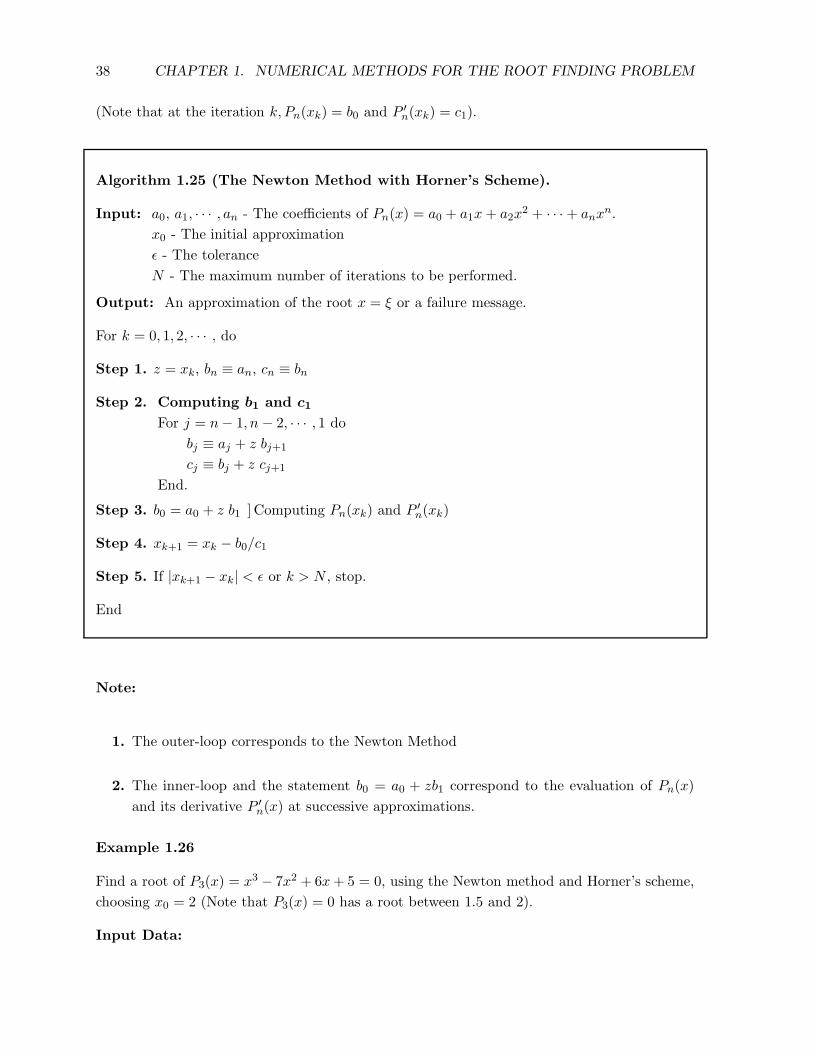
Algorithm 1.25 (The Newton Method with Horner’s Scheme).
Input: a0, a1, · · · , an - The coefficients of Pn(x) = a0 + a1x+ a2x2 + · · ·+ anx
n.
x0 - The initial approximation
ǫ - The tolerance
N - The maximum number of iterations to be performed.
Output: An approximation of the root x = ξ or a failure message.
For k = 0, 1, 2, · · · , do
Step 1. z = xk, bn ≡ an, cn ≡ bn
Step 2. Computing b1 and c1
For j = n− 1, n − 2, · · · , 1 do
bj ≡ aj + z bj+1
cj ≡ bj + z cj+1
End.
Step 3. b0 = a0 + z b1 ] Computing Pn(xk) and P ′n(xk)
Step 4. xk+1 = xk − b0/c1
Step 5. If |xk+1 − xk| < ǫ or k > N , stop.
End
Note:
1. The outer-loop corresponds to the Newton Method
2. The inner-loop and the statement b0 = a0 + zb1 correspond to the evaluation of Pn(x)
and its derivative P ′n(x) at successive approximations.
Example 1.26
Find a root of P3(x) = x3 − 7x2 + 6x+ 5 = 0, using the Newton method and Horner’s scheme,
choosing x0 = 2 (Note that P3(x) = 0 has a root between 1.5 and 2).
Input Data:
1.10. THE MULLER METHOD: FINDING A PAIR OF COMPLEX ROOTS. 39
(i) The coefficients of P3(x): a0 = 5, a1 = 6, a2 = −7, and a3 = 1.
(ii) The degree of the polynomial: n = 3.
(iii) Initial approximation: x0 = 2.
Solution.
Iteration 1. (k = 0). Compute x1 from x0:
x1 = x0 −b0c1
= 2− 3
10=
17
10= 1.7
Note that b0 = P3(x0) and c1 = P ′3(x0) have already been computed in Example 1.23.
Iteration 2. (k = 1). Compute x2 from x1:
Step 1. z = x1 = 1.7, b3 = 1, c3 = b3 = 1
Step 2.
b2 = a2 + z b3 = −7 + 1.7 = −5.3
c2 = b2 + z c3 = −5.3 + 1.7 = −3.6
b1 = a1 + z b2 = 6 + 1.7(−5.3) = −3.0100
c1 = b1 + z c2 = −3.01 + 1.7(−3.6) = −9.130 (Value of P ′3(x1)).
Step 3. b0 = a0 + z b1 = 5 + 1.7(−3.0100) = −0.1170 (Value of P3(x1)).
Step 4. x2 = x1 −b0c1
= 1.7− 0.1170
9.130= 1.6872
(The exact root, correct up to four decimal places is 1.6872 ).
1.10 The Muller Method: Finding a Pair of Complex Roots.
TheMuller Method is an extension of the Secant Method. It is conveniently used to approximate
a complex root of a real equation, using real starting approximations or just a real root.
Note that none of the methods: the Newton, the Secant, the Fixed Point iteration Methods, etc.
can produce an approximation of a complex root starting from real approximations.
The Muller Method is capable of doing so.
Given two initial approximations, x0 and x1 the successive approximations are computed as
follows:
• Approximating x2 from x0 and x1: The approximation x2 is computed as the x-
intercept of the secant line passing through (x0, f(x0)) and (x1, f(x1)).
40 CHAPTER 1. NUMERICAL METHODS FOR THE ROOT FINDING PROBLEM
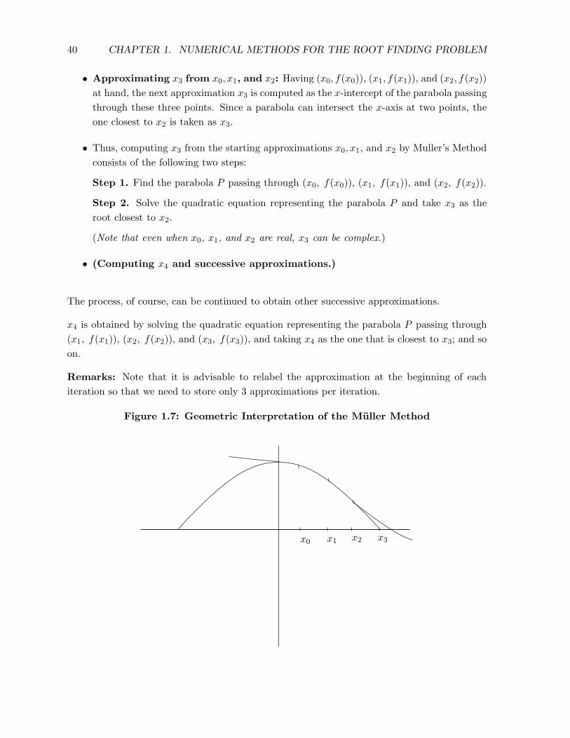
• Approximating x3 from x0, x1, and x2: Having (x0, f(x0)), (x1, f(x1)), and (x2, f(x2))
at hand, the next approximation x3 is computed as the x-intercept of the parabola passing
through these three points. Since a parabola can intersect the x-axis at two points, the
one closest to x2 is taken as x3.
• Thus, computing x3 from the starting approximations x0, x1, and x2 by Muller’s Method
consists of the following two steps:
Step 1. Find the parabola P passing through (x0, f(x0)), (x1, f(x1)), and (x2, f(x2)).
Step 2. Solve the quadratic equation representing the parabola P and take x3 as the
root closest to x2.
(Note that even when x0, x1, and x2 are real, x3 can be complex.)
• (Computing x4 and successive approximations.)
The process, of course, can be continued to obtain other successive approximations.
x4 is obtained by solving the quadratic equation representing the parabola P passing through
(x1, f(x1)), (x2, f(x2)), and (x3, f(x3)), and taking x4 as the one that is closest to x3; and so
on.
Remarks: Note that it is advisable to relabel the approximation at the beginning of each
iteration so that we need to store only 3 approximations per iteration.
Figure 1.7: Geometric Interpretation of the Muller Method
x0 x1 x2 x3
1.10. THE MULLER METHOD: FINDING A PAIR OF COMPLEX ROOTS. 41
Based on the above idea, we now give the details of how to obtain x3 starting from x0, x1, and
x2.
Let the equation of the parabola P be
P (x) = a(x− x2)2 + b(x− x2) + c.
That is, P (x2) = c, and a and b are computed as follows:
Since P (x) passes through (x0, f(x0)), (x1, f(x1)), and (x2, (f(x2)), we have
P (x0) = f(x0) = a(x0 − x2)2 + b(x0 − x2) + c
P (x1) = f(x1) = a(x1 − x2)2 + b(x1 − x2) + c
P (x2) = f(x2) = c.
Knowing c = f(x2), we can now obtain a and b by solving the first two equations:
a(x0 − x2)2 + b(x0 − x2) = f(x0)− c
a(x1 − x2)2 + b(x1 − x2) = f(x1)− c.
]
Or(
(x0 − x2)2 (x0 − x2)
(x1 − x2)2 (x1 − x2)
)(
a
b
)
=
(
f(x0)− c
f(x1)− c
)
.
Knowing a and b from above, we can now obtain x3 by solving P (x3) = 0.
P (x3) = a(x3 − x2)2 + b(x3 − x2) + c = 0.
To avoid catastrophic cancellation (See Chapter 3), instead of using the traditional for-
mula, we use the following mathematical equivalent formula for solving the quadratic equation
ax2 + bx+ c = 0.
Solving the Quadratic Equation
ax2 + bx+ c = 0
x =−2c
b±√b2 − 4ac
The sign in the denominator is chosen so that it is the largest in magnitude, guaranteeing that
x3 is closest to x2.

42 CHAPTER 1. NUMERICAL METHODS FOR THE ROOT FINDING PROBLEM
To solve P (x3) = 0 using the above formula, we get
x3 − x2 =−2c
b±√b2 − 4ac
or x3 = x2 +−2c
b±√b2 − 4ac
.
Note: One can also give on explicit expressions for a and b as follows:
b =(x0 − x2)
2 [f(x1)− f(x2)]− (x1 − x2)2 [f(x0)− f(x2)]
(x0 − x2)(x1 − x2)(x0 − x1)
a =(x1 − x2) [f(x0)− f(x2)]− (x0 − x2) [f(x1)− f(x2)]
(x0 − x2)(x1 − x2)(x0 − x1).
However, for computational efficiency and accuracy, it is easier to solve the following 2 × 2
linear system (displayed in Step2-2 of Algorithm 1.27 below) to obtain a and b, once c = f(x2)
is computed.
Algorithm 1.27 (The Muller Method for Approximations of a Pair of Complex
Roots).
Input: f(x) - The given function
x0, x1, x2 - Initial approximations
ǫ - Tolerance
N - The maximum number of iterations
Output: An approximation of the root x = ξ
Step 1. Evaluate the functional values at the initial approximations: f(x0), f(x1),
and f(x2).
Step 2. Compute the next approximation x3 as follows:
2.1 Set c = f(x2).
2.2 Solve the 2× 2 linear system for a and b:
(
(x0 − x2)2 (x0 − x2)
(x1 − x2)2 (x1 − x2)
)(
a
b
)
=
(
f(x0)− c
f(x1)− c
)
.
2.3 Compute x3 = x2 +−2c
b±√b2 − 4ac
choosing the sign + or − so that the denomi-
nator is the largest in magnitude.
Step 3. Test if |x3 − x2| < ǫ or if the number of iterations exceeds N . If so, stop. Otherwise
go to Step 4.

1.10. THE MULLER METHOD: FINDING A PAIR OF COMPLEX ROOTS. 43
Step 4. Relabel x3 as x2, x2 as x1, and x1 as x0:
x2 ≡ x3
x1 ≡ x2
x0 ≡ x1Return to Step 1.
Example 1.28
(Approximating a Pair of Complex Roots by Muller’s Method) Approximate a pair of
complex roots of x3 − 2x2 − 5 = 0 starting with the initial approximations as x0 = −1, x1 = 0,
and x2 = 1. (Note the roots of f(x) = {2.6906,−0.3453 ± 1.31876}.)
Input Data:
The function: f(x) = x3 − 2x2 − 5,
The initial approximations: x0 = −1, x1 = 0, x2 = 1
Formula to be used: x3 = x2 +−2c
b±√b2−4ac
,
Choosing + or − to obtain the largest (in magnitude) denominator.
Solution.
Iteration 1.
Step 1. Compute the functional values. f(x0) = −8, f(x1) = −5, f(x2) = −6.
Step 2. Compute the next approximation x3 as follows:
2.1 Set c: c = f(x2) = −6
2.2 Compute a and b: a and b are obtained by solving the 2× 2 linear system:
4a− 2b = −2
a− b = 1
]
⇒ a = −2, b = −3
2.3 Compute x3:
x3 = x2 −2c
b−√b2 − 4ac
= x2 +12
−3−√9− 48
= 0.25 + 1.5612i.
Iteration 2. Relabel x3 as x2, x2 as x1, and x1 as x0:
x2 ≡ x3 = 0.25 + 1.5612i
x1 ≡ x2 = 1
x0 ≡ x1 = 0

44 CHAPTER 1. NUMERICAL METHODS FOR THE ROOT FINDING PROBLEM
Step 1. Compute the new functional values: f(x0) = −5, f(x1) = −6, and f(x2) =
−2.0625 − 5.0741i
Step 2. Compute the next approximation x3:
2.1 Set c = f(x2).
2.2 Obtain a and b by solving the 2× 2 linear system:
(
x22 −x2
(x1 − x2)2 (x1 − x2)
)(
a
b
)
=
(
f(x0)− c
f(x1)− c
)
,
which gives a = −0.75 + 1.5612i, b = −5.4997 − 3.1224i.
2.3 x3 = x2 −2c
b−√b2 − 4ac
= x2 − (0.8388 + 0.3702i) = −0.5888 + 1.1910i
Iteration 3. Relabel x3 as x2, x2 as x1, and x1 as x0:
x2 ≡ x3 = −0.5888 + 1.1910i
x1 ≡ x2 = 0.25 + 1.5612i
x0 ≡ x1 = 1
Step 1. Compute the functional values: f(x0) = −6, f(x1) = −2.0627 − 5.073i, f(x2) =
−0.5549 + 2.3542i
Step 2. Compute the new approximation x3:
2.1 Set c = f(x2).
2.2 Obtain a and b by solving the 2× 2 system:
(
(x0 − x2)2 (x0 − x2)
(x1 − x2)2 (x1 − x2)
)(
a
b
)
=
(
f(x0)− c
f(x1)− c
)
,
which gives a = −1.3888 + 2.7522i and b = −2.6339 − 8.5606i.
3 x3 = x2 −2c
b−√b2 − 4ac
= −0.3664 + 1.3508i
Iteration 4. x3 = −0.3451 + 1.3180i (Details computations are similar and not shown)
Iteration 5. x3 = −0.3453 + 1.3187i
Iteration 6. x3 = 0.3453 + 1.3187i
Test for Convergence:
∣
∣
∣
∣
x3 − x2x2
∣
∣
∣
∣
< 5.1393 × 10⁻⁴, we stop here and accept the latest value
of x3 as an approximation to the root.

1.10. THE MULLER METHOD: FINDING A PAIR OF COMPLEX ROOTS. 45
Thus, an approximate pair of complex roots is:
α1 = −0.3455 + 1.3187i, α2 = −0.3455 − 1.3187i.
Verify: How close is this root to the actual root? (x−α1)(x−α2)(x−2.6906) = x3−1.996x2−5
Example 1.29
(Approximating a Real Root by Muller’s Method)
Approximate a real root of f(x) = x3 − 7x2 +6x+5 using x0 = 0, x1 = 1, and x2 = 2 as initial
approximations. (All three roots are real: 5.8210, 1.6872, −0.5090. We will try to approximate
the root 1.6872).
Input Data:
f(x) = x3 − 7x2 + 6x+ 5
Initial approximations: x0 = 0, x1 = 1, and x2 = 2.
Solution.
Iteration 1. Compute x3 from x0, x1, and x2:
Step 1. The functional values at the initial approximations: f(x0) = 5, f(x1) =
5, f(x2) = −3.
Step 2. Compute the next approximation x3:
2.1 Compute c = f(x2) = −3.
2.2 Compute a and b by solving the 2× 2 linear system:(
(x0 − x2)2 (x0 − x2)
(x1 − x2)2 (x1 − x2)
)(
a
b
)
=
(
5− c
5− c
)
or(
4 −2
1 −1
)(
a
b
)
=
(
8
8
)
⇒
a = −4
b = −12
2.3 Compute x3 = x2 −2c
b−√b2 − 4ac
x3 = x2 − 0.2753 = 1.7247 (choosing the negative sign in the determinant).
Iteration 2. Relabel x3 as x2, x2 as x1, and x1 as x0:
x2 ≡ x3 = 1.7247,
x1 ≡ x2 = 2,
x0 ≡ x1 = 1

46 CHAPTER 1. NUMERICAL METHODS FOR THE ROOT FINDING PROBLEM
Step 1. Compute the functional values at the relabeled approximations: f(x0) = 5,
f(x1) = −3, f(x2) = −0.3441
Step 2. Compute the new approximation x3:
2.1 Set c = f(x2) = −0.3441.
2.2 Then a and b are obtained by solving the 2× 2 linear system:
(
0.5253 −0.7247
0.0758 0.2753
)(
a
b
)
=
(
5− c
3− c
)
,⇒
a = −2.2752
b = −9.0227
2.3 x3 = x2 −2c
b−√b2 − 4ac
= 1.7247 − 0.0385 = 1.6862
1.10. THE MULLER METHOD: FINDING A PAIR OF COMPLEX ROOTS. 47
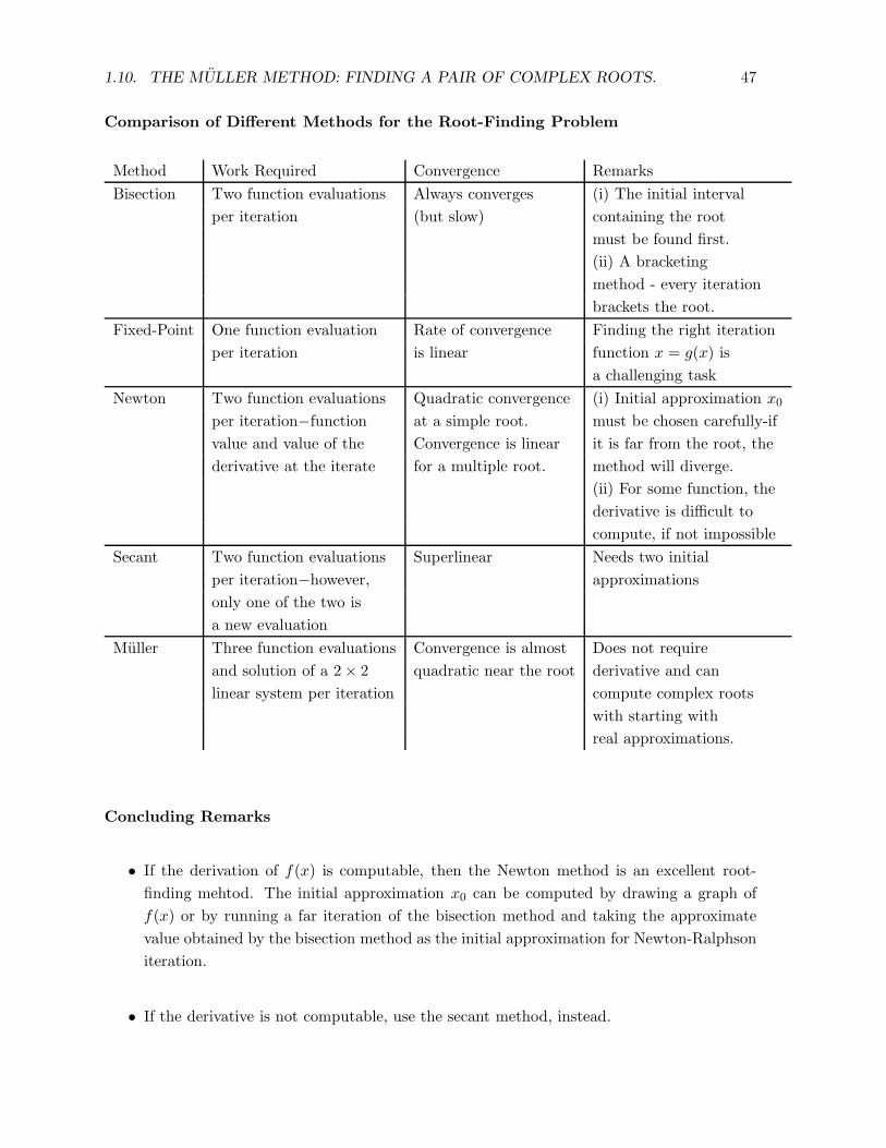
Comparison of Different Methods for the Root-Finding Problem
Method Work Required Convergence Remarks
Bisection Two function evaluations Always converges (i) The initial interval
per iteration (but slow) containing the root
must be found first.
(ii) A bracketing
method - every iteration
brackets the root.
Fixed-Point One function evaluation Rate of convergence Finding the right iteration
per iteration is linear function x = g(x) is
a challenging task
Newton Two function evaluations Quadratic convergence (i) Initial approximation x0
per iteration−function at a simple root. must be chosen carefully-if
value and value of the Convergence is linear it is far from the root, the
derivative at the iterate for a multiple root. method will diverge.
(ii) For some function, the
derivative is difficult to
compute, if not impossible
Secant Two function evaluations Superlinear Needs two initial
per iteration−however, approximations
only one of the two is
a new evaluation
Muller Three function evaluations Convergence is almost Does not require
and solution of a 2× 2 quadratic near the root derivative and can
linear system per iteration compute complex roots
with starting with
real approximations.
Concluding Remarks
• If the derivation of f(x) is computable, then the Newton method is an excellent root-
finding mehtod. The initial approximation x0 can be computed by drawing a graph of
f(x) or by running a far iteration of the bisection method and taking the approximate
value obtained by the bisection method as the initial approximation for Newton-Ralphson
iteration.
• If the derivative is not computable, use the secant method, instead.
48 CHAPTER 1. NUMERICAL METHODS FOR THE ROOT FINDING PROBLEM
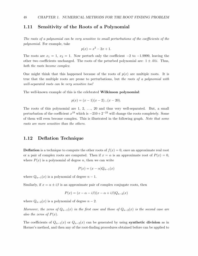
1.11 Sensitivity of the Roots of a Polynomial
The roots of a polynomial can be very sensitive to small perturbutions of the coefficients of the
polynomial. For example, take
p(x) = x2 − 2x+ 1.
The roots are x1 = 1, x2 = 1. Now perturb only the coefficient −2 to −1.9999, leaving the
other two coefficients unchanged. The roots of the peturbed polynomial are: 1 ± .01i. Thus,
both the roots become complex.
One might think that this happened because of the roots of p(x) are multiple roots. It is
true that the multiple roots are prone to perturbations, but the roots of a polynomial with
well-separated roots can be very sensitive too!
The well-known example of this is the celebrated Wilkinson polynomial:
p(x) = (x− 1)(x− 2)...(x − 20).
The roots of this polynomial are 1, 2, . . ., 20 and thus very well-separated. But, a small
perturbation of the coefficient x19 which is −210+2−23 will change the roots completely. Some
of them will even become complex. This is illustrated in the following graph. Note that some
roots are more sensitive than the others.
1.12 Deflation Technique
Deflation is a technique to compute the other roots of f(x) = 0, once an approximate real root
or a pair of complex roots are computed. Then if x = α is an approximate root of P (x) = 0,
where P (x) is a polynomial of degree n, then we can write
P (x) = (x− α)Qn−1(x)
where Qn−1(x) is a polynomial of degree n− 1.
Similarly, if x = α± iβ is an approximate pair of complex conjugate roots, then
P (x) = (x− α− iβ)(x− α+ iβ)Qn−2(x)
where Qn−2(x) is a polynomial of degree n− 2.
Moreover, the zeros of Qn−1(x) in the first case and those of Qn−2(x) is the second case are
also the zeros of P (x).
The coefficients of Qn−1(x) or Qn−2(x) can be generated by using synthetic division as in
Horner’s method, and then any of the root-finding procedures obtained before can be applied to

1.12. DEFLATION TECHNIQUE 49
Figure 1.8: Roots of the Wilkinson Polynomial (Original and Perturbed)
0 5 10 15 20 25−4
−3
−2
−1
0
1
2
3
4
Re
ImRoots of Wilkinson polynomial
originalperturbed
compute a root or a pair of roots of Qn−2(x) = 0 or Qn−1(x). The procedure can be continued
until all the roots are found.
Example 1.30
Find the roots of f(x) = x4 + 2x3 + 3x2 + 2x+ 2 = 0.
It is easy to see that x = ±i is a pair of complex conjugate roots of f(x) = 0. Then we can
write
f(x) = (x+ i)(x− i)(b3x2 + b2x+ b1)
or
x4 + 2x3 + 3x2 + 2x+ 2 = (x2 + 1)(b3x2 + b2x+ b1).
Equating coefficients of x4 , x3, and x2 on both sides, we obtain
b3 = 1, b2 = 2, b1 + b3 = 3,
giving b3 = 1, b2 = 2, b1 = 2.
So, (x4 + 2x3 + 3x2 + 2x+ 2) = (x2 + 1)(x2 + 2x+ 2).

50 CHAPTER 1. NUMERICAL METHODS FOR THE ROOT FINDING PROBLEM
Thus the roots of the polynomial equation: x4 + 2x3 + 2x2 + 2x + 2 are given by the roots of
(i) x2 + 1 = 0 and (ii) x2 + 2x+ 2.
The zeros of the deflated polynomial Q2(x) = x2 + 2x + 2 can now be found by using any of
the methods described earlier.
1.13 MATLAB Functions for Root-Finding
MATLAB built-in functions fzero, poly, polyval, and roots can be used in the context of
zero-finding of a function.
In a MATLAB setting, type help follwed by these function names, to know the details of the
uses of these functions. Here are some basic uses of these functions.
A. Function fzero: Find the zero of f(x) near x0. No derivative is required.
Usage:
y = fzero (function, x0).
function − Given function (specified either as a MATLAB function file or as
an anonymous function).
x0 − A point near the zero of f(x), if it is a scalar.
x0 − If given as a 2-vector,
[
a
b
]
then it is assumed that f(x) has a zero
in the interval [a, b].
• The function fzero can also be used with options to display the optimal requirements
such as values of x and f(x) at each iteration (possibly with some specified tolerance).
For example, the following usages:
options = optimset (’Display’, ’iter’)
z = fzero (function, x0, options)
or
z = fzero (function, x, optimset (’Display’, ’iter’). will display the value of x and the
corresponding value of f(x) at each iteration performed (see below Exercise 1.31). Other
values of options are also possible.
Example 1.31 (i) Find the zero of f(x) = ex − 1 near x = 0.1.
(ii) Find the zero of f(x) = ex−1 in [−1, 2] and display the values of x and f(x) at each
iteration.
Solution (i)
1.13. MATLAB FUNCTIONS FOR ROOT-FINDING 51
z = fzero (@(z) exp(x)− 1, 0.1)
z = 0.
Solution (ii)
z = fzero (@(x) exp(x)− 1, [−1, 2]T )
z = 2.1579e−17
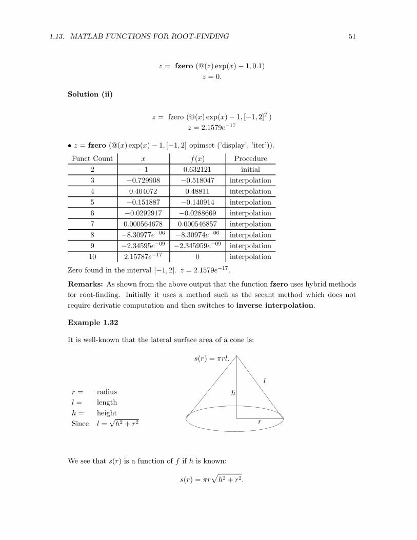
• z = fzero (@(x) exp(x)− 1, [−1, 2] opimset (’display’, ’iter’)).
Funct Count x f(x) Procedure
2 −1 0.632121 initial
3 −0.729908 −0.518047 interpolation
4 0.404072 0.48811 interpolation
5 −0.151887 −0.140914 interpolation
6 −0.0292917 −0.0288669 interpolation
7 0.000564678 0.000546857 interpolation
8 −8.30977e−06 −8.30974e−06 interpolation
9 −2.34595e−09 −2.345959e−09 interpolation
10 2.15787e−17 0 interpolation
Zero found in the interval [−1, 2]. z = 2.1579e−17 .
Remarks: As shown from the above output that the function fzero uses hybrid methods
for root-finding. Initially it uses a method such as the secant method which does not
require derivatie computation and then switches to inverse interpolation.
Example 1.32
It is well-known that the lateral surface area of a cone is:
s(r) = πrl.
h
r
l
r = radius
l = length
h = height
Since l =√h2 + r2
We see that s(r) is a function of f if h is known:
s(r) = πr√
h2 + r2.

52 CHAPTER 1. NUMERICAL METHODS FOR THE ROOT FINDING PROBLEM
Find the radius of the cone whose lateral surface area is 750m2 and the height is 9m,
using MATLAB function fzero.
Solution
We need to find a zero r of the function:
f(r) = 750 − πr√
r2 + 9
Choose r0 = 5.
r = fzero (@(r)750 − π ∗ r ∗ sqrt+ (r2 + 9), 5)
r = 15.3060.
So, the radius of the cone should be 15.3060m.
B. Functions: poly, polyval, and roots.
These functions relate to finding the roots of a polynomial equation.
poly - converts roots to a polynomial equation.
• poly (A), when A is an n×n matrix, gives a row vector with (n+1) elements which
are the coefficients of the characteristic polynomial
P (λ) = det(λI −A)
• poly (v), when v is a vector, gives a vector whose elements are the coefficients of the
polynomial whose roots are the elements of v.
roots - Find the polynomial roots.
• roots (c) computes the roots of the polynomial whose coefficients are the elements of
the vector c:
P (x) = c1xn + c2x
n−1 + · · ·+ cnx+ cx+1
polyval - Evaluates the value of a polynomial at a given point.
• y = polyval (p, z) returns the value of a polynomial P (x) at x = z.
where
p = the vector containing the coefficients (c1, c2, . . . , cn+1) of the polynomial P (x) as above.
z = a number, a vector, or a matrix.
If it is a vector or matrix, P (x) is evaluated at all points in z.
Example 1.33
Using the functions poly, roots, and polyval,

1.13. MATLAB FUNCTIONS FOR ROOT-FINDING 53
(i) Find the coefficients of the polynomial equation P3(x) whose roots are: 1, 1, 2, and
3.
(ii) Compute now, numerically, the roots and check the accuracy of each computed root.
(iii) Perturb the coefficient of x2 of P4(x) by 10−4 and recompute the roots.
Solution (i).
v = [1, 1, 2, 3]T
c = polyv
The vector c contains the coefficients of the 4-th degree polynomial P4(x) with the roots:
1,1,2, and 3.
c = [1,−7, 17,−17, 6]T
P4(x) = x4 − 7x3 + 17x2 − 17x+ 6
Solution (ii).
z = roots (c) gives the computed zeros of the polynomial P4(x).
z =
3.0000
2.0000
1.0000
1.0000
Solution (iii).
Perturbed polynomial P4(x) is given by
P4(x) = x4 − (7 + 10−4)x3 + 17x2 − 17x+ 6
The vector cc containing the coefficients of P4(x) is given by:
cc = [ ]T
zz = roots (cc).
The vector zz contains the zeros of the perturbed polynomial P4(x):
vv = polyval (zz).
The vector vv contains the values of P4(x) evaluated at the computed roots of P4(x):
vv = [ ]T
54 CHAPTER 1. NUMERICAL METHODS FOR THE ROOT FINDING PROBLEM
• Function eig.
• eig(A) is used to compute the eigenvalues of a matrix A. It can be used to find all the roots
of a polynomial, as the following discussions show.
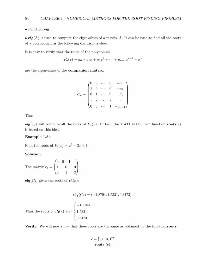
It is easy to verify that the roots of the polynomial
Pn(x) = a0 + a1x+ a2x2 + · · · + an−1x
n−1 + xn
are the eigenvalues of the companion matrix.
Cn =
0 0 · · · 0 −a0
1 0 · · · 0 −a1
0 1 · · · 0 −a2...
.... . .
......
0 0 · · · 1 −an−1
Thus,
eig(cn) will compute all the roots of Pn(x). In fact, the MATLAB built-in function roots(c)
is based on this idea.
Example 1.34
Find the roots of P3(x) = x3 − 3x+ 1.
Solution.
The matrix c3 =
0 0− 1
1 0 0
0 1 3
.
eig(C3) gives the roots of P3(x):
eig(C3) = (−1.8794, 1.5321, 0.3473).
Thus the roots of P3(x) are:
−1.8784
1.5321
0.3473
Verify: We will now show that these roots are the same as obtained by the function roots:
c = [1, 0, 3, 1]T
roots (c).

1.13. MATLAB FUNCTIONS FOR ROOT-FINDING 55
roots(c) =
−1.8784
1.5321
0.3473
same as obtained by eig(C3).
Remarks: It is not recommended that the eigenvalues of an arbitrary matrix A are com-
puted by transforming A first into companion form C and then finding its zeros. Because, the
transforming matrix can be highly ill-conditioned (Please see Chapter 8).

56 CHAPTER 1. NUMERICAL METHODS FOR THE ROOT FINDING PROBLEM
EXERCISES
0. (Conceptual) Answer True or False. Give reasons for your answer.
(i) Bisection method is guaranteed to find a root in the interval in which the root lies.
(ii) Bisection method converges quite fast.
(iii) It is possible to theoretically find the minimum number of iterations needed by
bisection method prior to starting the iteration.
(iv) Bisection method brackets the root in each iteration.
(v) Newton’s method always converges.
(vi) Quadratic convergence means that about two digits of accuracy are obtained at each
iteration.
(vii) Fixed point iteration always converges, but the rate of convergence is quite slow.
(viii) In the presence of a multiple root, Newton’s method does not converge at all.
(ix) The rate of convergence of Newton’s method, when it converges, is better than the
secant method.
(x) Both the secant and false-positive methods are bracket methods.
(xi) Horner’s scheme efficiently computes the value of a polynomial and its derivative at
a given point.
(xii) Muller’s method can compute a pair of complex conjugate roots using only real
approximations.
(xiii) Only the multiple roots of a polynomial equation are sensitive to small perturbations
of the data.
(xiv) The fixed-point iteration theorem (Theorem ??) gives both necessary and sufficient
conditions of the convergence of the fixed-point iteration to a root.
(xv) A computational advantage of the secant method is that the derivative of f(x) is
not required.
(xvi) Newton’s method is a special case of the fixed-point iteration scheme.
(xvii) Both Newton and second methods require two initial approximations to start the
iteration.
(xviii) The convergence rate of the standard Newton’s method for a multiple root is only
linear.
(xix) A small functional value at x = α guarantees that it is a root f(x) = 0.
1. Use the bisection method to approximate√3 with an error tolerance ǫ = 10−3 in the
intervals: [1, 2], [1, 3], and [0, 2].
1.13. MATLAB FUNCTIONS FOR ROOT-FINDING 57
2. (Computational) For each of the following functions, do the following:
(a) Test if there is a zero of f(x) in the indicated interval.
(b) Find the minimum number of iterations, N , needed to achieve an accuracy of ǫ =
10−3 by using the bisection method.
(c) Using the bisection method, perform N number of iterations and present the results
both in tabular and graphical forms.
(i) f(x) = x sinx− 1 in [0, 2]
(ii) f(x) = x3 − 1 in [0, 2]
(iii) f(x) = x2 − 4 sinx in [1, 3]
(iv) f(x) = x3 − 7x+ 6 in [0, 1.5]
(v) f(x) = cos x−√x in [0, 1]
(vi) f(x) = x− tanx in [4, 4.5]
(vii) f(x) = e−x − x in [0, 1]
(viii) f(x) = ex − 1− x− x2
2 in [−1, 1]
3.
4. (Computational) Construct a simple example to show that a small functional value of
f(xk) at an iteration k does not necessarily mean that xk is near the root x = ξ of f(x).
5. (Analytical)
(a) Prove that if g(x) is continuously differentiable in some open interval containing the
fixed point ξ, and if |g′(ξ) < 1, then there exists a number ǫ > 0 such that the
iteration
xk+1 = g(xk)
converges whenever x0 is chosen such that |x0 − ξ| ≤ ǫ.
(b) Using the above result, find the iteration function g(x) and an interval [a, b] for
f(x) = x− tan x
such that the iteration always converges. Find the solution with an accuracy of 10−4.
(c) Find a zero of the function f(x) = e−x−sinx in [0.5, 0.7], by choosing g(x) = x+f(x)
and using the result in (a).
6. (Computational) For each of the following functions, find an interval and an iteration
function x = g(x) so that the fixed-point iteration:
xk+1 = g(xk)
will converge for any choice of x0 in the interval. Then apply two iterations to approximate
a zero in that interval choosing a suitable initial approximation x0.

58 CHAPTER 1. NUMERICAL METHODS FOR THE ROOT FINDING PROBLEM
(a) f(x) = x− cosx
(b) f(x) = 3x2 − x− 2
(c) f(x) = x− e−x
(d) f(x) = x2 − 4 sin(x)
(e) f(x) = 1
1+e−x2+ cos x
(f) f(x) = x2
4 − 1
(g) f(x) = x− 2 sinx
(h) f(x) = x3 − 7x+ 6
(i) f(x) = 1− tan x4
7. (Computational) Use fixed-point iteration to compute√2 with an accuracy of 10−4.
8. (Computational) Study the convergence of all fixed-point iterations of the function f(x) =
x3−7x+6 at x = 2 with all possible iteration functions g(x). Represent these fixed point
iteration schemes graphically.
9. (Computational)
(a) Sketch a graph of f(x) = x+lnx and show that f(x) has one and only one zero ξ in
0 < x < ∞, but that the related fixed point iteration xi+1 = g(xi), x0 given, x0 6= ξ,
with g(x) = − lnx, does not converge to ξ even if x0 is arbitrarily close to ξ.
(b) How can one rewrite the iteration equation so as to obtain convergence? Show for
this iteration the uniqueness of the fixed point ξ. Give its rate of convergence.
10. (Computational) The iteration xn+1 = 2 − (1 + c)xn + cx3n will converge to ξ = 1 for
some values of c (provided x0 is chosen sufficiently close to ξ). Find the values of c for
which this is true. For what value of c will the convergence be quadratic?
11. (Computational) Apply Newton’s method, the secant method and the method of false
position to determine a zero with an accuracy of 10−4 to each of the functions in Exercise
6.
12. (Computational) Write down Newton’s iterations for the following functions:
(a) x3 − cos(x2 + 1) = 0
(b) 2 sin πx−√x2 − x+ 1 = 0
13. (Analytical and Computational) Develop Newton’s method to compute the following:
(a) ln(a) (natural log of a) (a > 0)
(b) arc cos a and arc sin a

1.13. MATLAB FUNCTIONS FOR ROOT-FINDING 59
(c) ea
Do three iterations for each problem by choosing a suitable function and a suitable x0.
Compare your results with those obtained by MATLAB built-in function fzero.
14. (Computational) Explain what happens when Newton’s method is applied to find a root
of x3 − 3x+ 6 = 0, starting with x0 = 1.
15. (Computational) Construct your own example to demonstrate the fact that Newton’s
method may diverge if x0 is not properly chosen.
16. (Computational) Show that the Newton sequence of iterations for the function f(x) =
x3 − 2x+2 with x0 = 0 will oscillate between 0 and 1. Give a graphical representation of
this fact.
Find now a positive root of f(x) using Newton’s method by choosing a suitable x0.
17. (Computational) Study the convergence behavior of Newton’s method to approximate
the zero x = 2 of the following two polynomials:
f(x) = x3 − 3x− 2
g(x) = x2 − 4x+ 4
starting with the same initial approximation x0 = 1.9.
18. (Computational) Write down the Newton-sequence of iterations to find a minimum or a
maximum of a function f(x).
Apply it to find the minimum value of f(x) = x2 + sinx
19. (Computational and Analytical) Derive an algorithm to compute n√A based on New-
ton’s method and apply your algorithm to compute 5√30, by choosing a suitable initial
approximation.
20. (Analytical and Computational) Repeat the previous problem with the secant method
and compare the speed of convergence.
21. (Analytical) Prove that the rate of convergence of Newton’s method for a multiple root
is only linear, not quadratic. Construct a small example to support this statement.
22. (Analytical) Prove that the convergence rate of the secant method is superlinear.
23. (Computational) Apply the secant method to f(x) = x3 − 3x + 2 to approximate the
root x = 1 with x0 = 0 and x1 = 2. Show that the convergence factor is approximately
1.6.
24. (Computational) The polynomial P3(x) = x3 − 2x2 + x − 2 has a pair of zeros x = +i.
Approximate them using Muller’s method.

60 CHAPTER 1. NUMERICAL METHODS FOR THE ROOT FINDING PROBLEM
25. (Computational) The polynomial P8(x) = x8+2x7+x6+2x5+5x3 +7x2+5x+7 has a
pair of complex-conjugate zeros x = ±i. Approximate them using Muller’s method (Do
three iterations.) Choose x0 = 0, x1 = 0.1, x2 = 0.5.
26. (Computational) The polynomial P6(x) = 3x6 − 7x3 − 8x2 + 12x + 3 = 0 has a double
root at x = −1. Approximate this root first by using standard Newton’s method and
then by two modified Newton’s methods, starting with x0 = −0.5.
Use Horner’s method to find the polynomial value and its derivative at each iteration.
Present your results in tabular form. (Do three iterations.)
27. (Applied) Consider the Kepler equation of motion
M = E − e sinE
relating the mean anomaly M to the eccentric anomaly E of an elliptic orbit with
eccentricity e. To find E, we need to solve the nonlinear equation:
f(E) = M + e sinE − E = 0
(a) Show that the fixed point iteration
E = g(E) = M + e sinE
converges.
(b) Given e = 0.0167 (Earth’s eccentricity)and M = 1 (in radians) compute E using
i. bisection method,
ii. fixed-point iteration E = g(E) as above,
iii. Newton’s method; and
iv. secant method.
To choose appropriate initial approximations or an interval containing the root (re-
quired for the bisection method), plot the function f(E) and then determine graph-
ically where it crosses the E-axis.
(c) Referring to the case study in Section 1.1, find the position of the planet Earth for
t = 300 days with a = 150× 106km.
28. (Applied) Consider the van der Walls equation of state:(
P +a
V 2
)
(V − b) = RT
Use Newton’s method to compute the specific volume V of carbon dioxide at a temperature
of T = 300oK, given P = 1 atom, R = 0.082054 J (kgoK), a = 3.592 Pa·m6/kg2, b =
0.04267m2/kg.
Obtain the initial approximation V0 from the ideal gas law: PV = RT .

1.13. MATLAB FUNCTIONS FOR ROOT-FINDING 61
29. (Applied) Repeat the last problem for oxygen for which a = 1.360 and b = 0.03183.
30. (Applied) Windmill Electric Power
It is becoming increasingly common to use wind turbines to generate electric power. The
energy output of the power generated by a windmill depends upon the blade’s diameter
and velocity of the wind. A good estimate of the energy output is given by the following
formula:
EO = 0.01328D2V 3
where EO = Energy Output, D = Diameter of the windmill blade (m), V = Velocity of
the wind in m/s.
Use Newton’s method to determine what should be the diameter of the windmill blade if
one wishes to generate 500 watts of electric power when the wind speed is 10mph.
31. (Applied) A spherical tank of radius r = Λm contains a liquid of volume V = 0.5m3.
What is the depth, h, of the liquid?
Use the following formula: V = πh2
3 (3r − h) to solve.
32. (Applied) If the displacement of a body at time t is given by
x(t) = cos 10t− 1
2sin 10t
At what time t(s) will the displacement be 20 meters?
33. (Applied) Suppose that the displacement of a body at time t under a damping oscillation
is given by
x(t) = e−t
(
A cos
√12
2t+B sin
√12
2t
)
Determine the time required for the body to come to rest (x(t) = 0) using the initial
conditions: x(0) = 1, x′(0) = 5.
(Hints: First, find A and B using the initial conditions. Then solve the above equation
for t setting x(t) = 0.)
34. (Analytical and Computational) (Haley’s Method) The following iteration for finding
a root of f(x) = 0:
xi+1 = xi −2f(xi)f
′(xi)2[f(xi)2 − f(xi)f
′′(xi)]
is known as Haley’s iteration.

62 CHAPTER 1. NUMERICAL METHODS FOR THE ROOT FINDING PROBLEM
(i) Prove that if f(x) is three times continuously differentiable and x = ξ is a root of
f(x) = 0; but not of its derivative, then Haley’s iteration converges to the zero if the
initial approximation x0 is sufficiently close to ξ, and that the convergence is cubic;
that is,
ei+1
e3i≤ C, for some C > 0
(ii) Using Haley’s iteration, compute a positive zero of f(x) = x3 − 3x+1 starting with
x0 = 0.5 with an error tolerance of ǫ = 10−4.

1.13. MATLAB FUNCTIONS FOR ROOT-FINDING 63
MATLAB EXERCISES
M1.1 Write MATLAB functions in the following formats to implement the methods: Bisec-
tion, Fixed-Point Iteration, Newton, Secant, and Muller.
• function [xval, funval, iter, error] = bisect(fnc, intv, tol, maxitr)
• function [xval, funval, iter, erro] = newton(fnc, deriv, x0, to, maxitr)
• function [ xval, funval, iter, error] = fixed-point(fnc, x0, tol, maxitr)
• function [xval,funval,iter, error] = secant(fnc, x0, x1, tol, maxitr)
• function [xval, funval, iter, error] = muller(fnc, x0, x1, x2, tol, maxitr)
intv = Interval containing the root
xval = Value of the root at the present iteration
iter = Iteration number
funval = Value of the function at the present iteration
error = Error message in case of nonconvergence
fnc = The function input as a string
deriv = Derivative of function also given as a string
xo, x1, x2 = Initial approximations
tol = Error tolerance
maxitr = Maximum number of iterations to be performed
fncval = Function value of the root at each iteration
Presentation of Results: Present your results both in tabular and graphic forms. The
tables and graphs should display the values of the function and the approximate root at
each iteration. Results from all the methods need to be presented in the same table and
same graph.
Table : Comparison of Different Root-Finding Methods
Method Iteration x-Value Function Value
Data: Implement the methods using the functions given in Exercises 6(a), 6(b), 6(d),
6(e), 6(h), and 6(i).
M1.2 Apply now the built-in MATLAB function fzero to the function of Exercise 2 and present
your results along with those of other methods in the same table and same graph using
the format of M1.1.
64 CHAPTER 1. NUMERICAL METHODS FOR THE ROOT FINDING PROBLEM
M1.3 Write a MATLAB program, using the built-in MATLAB functions, polyval, and poly-
der to find a zero of a polynomial, based on Newton’s Method with Horner’s scheme.
Implement the program using
P (x) = x5 − x4 − 5x3 − x2 + 4x+ 3
Present results of each iteration both in tabular and graphic forms.
M1.4 Choosing the values of a, b, R and P in appropriate units, find v at temperatures
T = 100oK, T = 250oK, T = 450oK by solving the Van der Waals equation state using
each of the methods developed in M1.1. Present the results in tabular form.
M1.5 Apply the MATLAB program newton to compute (a) 5√1000 and (b) 1
12000 , (c) e5,
and (d) ln(10), choosing a suitable initial approximation in each case. For each problem,
present your results of iterations in tabular forms.
M1.6 Consider the following equation:
A =R
i
[
1 = (1 + i)−n]
where A = Amount of money borrowed; i = Interest rate per time period; R = Amount
of each payment; n = Number of payments (all payments are of equal value).
If the amount of the loan is $20,000 and the payment amount per month is $450.00 and
the loan is paid off in 5 years, what is the monthly interest rate? (Solve the problem using
the newton program.)
M1.7 The following formula gives the upward velocity v of a rocket:
v = u lnm
m− qt− gt
where u = The velocity of the fuel expelled relative to the rocket; m = Initial mass of the
rocket (at t = 0); g = Gravity’s acceleration; t = Time.
Use any bracket method to find the time taken by the rocket to attain the velocity of 500
m/s, given
u = 950 m/s, m = 2× 10⁵ kg, q = 3, 000 kg/s, and g = 9.8 m/s2.
Choose 10 ≤ t ≤ 25.
M1.8 Suppose the concentration c of a chemical in a mixed reactor is given by:
c = cin(1− e−0.05t) + c0e−0.05t
where cin = Inflow concentration; and c0 = Original concentration.
Find the time t required for c to be 90% of cin, if c0 = 5, and cin = 15.

1.13. MATLAB FUNCTIONS FOR ROOT-FINDING 65
M1.9 Display the results of the following MATLAB operations:
f = inline (’3/x2 − x− 2’)
fzero = (f, 1.5, optimset(’display’, ’iter’))
Interpret. What do these results mean?
M1.10 (Study of the Root-Sensitivities of Polynomials)
Using MATLAB functions, roots, poly, and polyval, do the following for each of the
following polynomials.
A. Compute all the zeros of the unperturbed polynomial.
B. Put perturbations of orders 10−3, 10−4, and 10−5 to the second highest coefficient
and recompute the zeros of each of the perturbed polynomial.
C. Present your results in tabular form that should contain (i) all the zeros of the
original, (ii) zeros of the perturbed polynomials with each perturbation and, (iii)
functional values at each computed zero.
D. Plot the zeros of the original and perturbed polynomials on the same graph for each
polynomial.
E. Write your observations in each case.
Data:
(i) The polynomial P20(x) with the zeros 1, 2, 3, 4, . . . , 20.
(ii) The polynomial P3(x) with all the zeros equal to 1.
(iii) The polynomial P4(x) with two doable zeros equal to 1 and two other zeros as 10
and 20.
M1.11 Modify the program Muller to accommodate deflation for computing more than one
root.
The polynomial
P7(x) = x7 − 41x6 + 690x5 − 6130x4 + 30689x3 − 84969x2 + 1116460x − 56700
has zeros: 10, 9, 7, 6, 5, 3, and 1.
Compute approximations to all of them using Muller’s method and the technique of
deflation.

66 CHAPTER 1. NUMERICAL METHODS FOR THE ROOT FINDING PROBLEM