University of Alabama at BirminghamDepartment of Mathematics

Numerical Linear Algebra

Lecture Notes for MA 660(1997–2014)

Dr Nikolai Chernov

Summer 2014

Contents

0. Review of Linear Algebra 10.1 Matrices and vectors . . . . . . . . . . . . . . . . . . . . . . . . . . . . . . 10.2 Product of a matrix and a vector . . . . . . . . . . . . . . . . . . . . . . . 10.3 Matrix as a linear transformation . . . . . . . . . . . . . . . . . . . . . . . 20.4 Range and rank of a matrix . . . . . . . . . . . . . . . . . . . . . . . . . . 20.5 Kernel (nullspace) of a matrix . . . . . . . . . . . . . . . . . . . . . . . . . 20.6 Surjective/injective/bijective transformations . . . . . . . . . . . . . . . . . 20.7 Square matrices and inverse of a matrix . . . . . . . . . . . . . . . . . . . . 30.8 Upper and lower triangular matrices . . . . . . . . . . . . . . . . . . . . . . 30.9 Eigenvalues and eigenvectors . . . . . . . . . . . . . . . . . . . . . . . . . . 40.10 Eigenvalues of real matrices . . . . . . . . . . . . . . . . . . . . . . . . . . 40.11 Diagonalizable matrices . . . . . . . . . . . . . . . . . . . . . . . . . . . . . 50.12 Trace . . . . . . . . . . . . . . . . . . . . . . . . . . . . . . . . . . . . . . . 50.13 Transpose of a matrix . . . . . . . . . . . . . . . . . . . . . . . . . . . . . . 60.14 Conjugate transpose of a matrix . . . . . . . . . . . . . . . . . . . . . . . . 60.15 Convention on the use of conjugate transpose . . . . . . . . . . . . . . . . 6

1. Norms and Inner Products 71.1 Norms . . . . . . . . . . . . . . . . . . . . . . . . . . . . . . . . . . . . . . 71.2 1-norm, 2-norm, and ∞-norm . . . . . . . . . . . . . . . . . . . . . . . . . 71.3 Unit vectors, normalization . . . . . . . . . . . . . . . . . . . . . . . . . . . 81.4 Unit sphere, unit ball . . . . . . . . . . . . . . . . . . . . . . . . . . . . . . 81.5 Images of unit spheres . . . . . . . . . . . . . . . . . . . . . . . . . . . . . 81.6 Frobenius norm . . . . . . . . . . . . . . . . . . . . . . . . . . . . . . . . . 81.7 Induced matrix norms . . . . . . . . . . . . . . . . . . . . . . . . . . . . . . 91.8 Computation of ‖A‖1, ‖A‖2, and ‖A‖∞ . . . . . . . . . . . . . . . . . . . . 91.9 Inequalities for induced matrix norms . . . . . . . . . . . . . . . . . . . . . 91.10 Inner products . . . . . . . . . . . . . . . . . . . . . . . . . . . . . . . . . . 101.11 Standard inner product . . . . . . . . . . . . . . . . . . . . . . . . . . . . . 101.12 Cauchy-Schwarz inequality . . . . . . . . . . . . . . . . . . . . . . . . . . . 111.13 Induced norms . . . . . . . . . . . . . . . . . . . . . . . . . . . . . . . . . . 121.14 Polarization identity . . . . . . . . . . . . . . . . . . . . . . . . . . . . . . . 121.15 Orthogonal vectors . . . . . . . . . . . . . . . . . . . . . . . . . . . . . . . 121.16 Pythagorean theorem . . . . . . . . . . . . . . . . . . . . . . . . . . . . . . 121.17 Orthogonality and linear independence . . . . . . . . . . . . . . . . . . . . 121.18 Orthonormal sets of vectors . . . . . . . . . . . . . . . . . . . . . . . . . . 131.19 Orthonormal basis (ONB) . . . . . . . . . . . . . . . . . . . . . . . . . . . 131.20 Fourier expansion . . . . . . . . . . . . . . . . . . . . . . . . . . . . . . . . 131.21 Orthogonal projection . . . . . . . . . . . . . . . . . . . . . . . . . . . . . . 131.22 Angle between vectors . . . . . . . . . . . . . . . . . . . . . . . . . . . . . . 141.23 Orthogonal projection onto a subspace . . . . . . . . . . . . . . . . . . . . 141.24 Degenerate case . . . . . . . . . . . . . . . . . . . . . . . . . . . . . . . . . 141.25 Gram-Schmidt orthogonalization . . . . . . . . . . . . . . . . . . . . . . . . 15

ii

1.26 Construction of ONB . . . . . . . . . . . . . . . . . . . . . . . . . . . . . . 151.27 Legendre polynomials (optional) . . . . . . . . . . . . . . . . . . . . . . . . 151.28 Orthogonal complement . . . . . . . . . . . . . . . . . . . . . . . . . . . . . 161.29 Orthogonal direct sum . . . . . . . . . . . . . . . . . . . . . . . . . . . . . 161.30 Some useful formulas . . . . . . . . . . . . . . . . . . . . . . . . . . . . . . 16

2. Unitary Matrices 182.1 Isometries . . . . . . . . . . . . . . . . . . . . . . . . . . . . . . . . . . . . 182.2 Characterization of isometries - I . . . . . . . . . . . . . . . . . . . . . . . 182.3 Characterization of isometries - II . . . . . . . . . . . . . . . . . . . . . . . 182.4 Characterization of isometries - III . . . . . . . . . . . . . . . . . . . . . . 182.5 Identification of finite-dimensional inner product spaces . . . . . . . . . . . 192.6 Unitary and orthogonal matrices . . . . . . . . . . . . . . . . . . . . . . . . 192.7 Lemma . . . . . . . . . . . . . . . . . . . . . . . . . . . . . . . . . . . . . . 192.8 Matrices of isometries . . . . . . . . . . . . . . . . . . . . . . . . . . . . . . 202.9 Group property . . . . . . . . . . . . . . . . . . . . . . . . . . . . . . . . . 202.10 Orthogonal matrices in 2D . . . . . . . . . . . . . . . . . . . . . . . . . . . 202.11 Characterizations of unitary and orthogonal matrices . . . . . . . . . . . . 212.12 Determinant of unitary matrices . . . . . . . . . . . . . . . . . . . . . . . . 212.13 Eigenvalues of unitary matrices . . . . . . . . . . . . . . . . . . . . . . . . 212.14 Invariance principle for isometries . . . . . . . . . . . . . . . . . . . . . . . 222.15 Orthogonal decomposition for complex isometries . . . . . . . . . . . . . . 222.16 Lemma . . . . . . . . . . . . . . . . . . . . . . . . . . . . . . . . . . . . . . 232.17 Orthogonal decomposition for real isometries . . . . . . . . . . . . . . . . . 232.18 Unitary and orthogonal equivalence . . . . . . . . . . . . . . . . . . . . . . 242.19 Unitary matrices in their simples form . . . . . . . . . . . . . . . . . . . . 242.20 Orthogonal matrices in their simples form . . . . . . . . . . . . . . . . . . 24

3. Hermitian Matrices 263.1 Adjoint matrices . . . . . . . . . . . . . . . . . . . . . . . . . . . . . . . . . 263.2 Adjoint transformations . . . . . . . . . . . . . . . . . . . . . . . . . . . . . 263.3 Riesz representation theorem . . . . . . . . . . . . . . . . . . . . . . . . . . 273.4 Quasi-linearity . . . . . . . . . . . . . . . . . . . . . . . . . . . . . . . . . . 273.5 Remark . . . . . . . . . . . . . . . . . . . . . . . . . . . . . . . . . . . . . . 273.6 Existence and uniqueness of adjoint transformation . . . . . . . . . . . . . 273.7 Relation between KerT ∗ and RangeT . . . . . . . . . . . . . . . . . . . . . 283.8 Selfadjoint operators and matrices . . . . . . . . . . . . . . . . . . . . . . . 283.9 Examples . . . . . . . . . . . . . . . . . . . . . . . . . . . . . . . . . . . . . 283.10 Hermitian property under unitary equivalence . . . . . . . . . . . . . . . . 283.11 Invariance principle for selfadjoint operators . . . . . . . . . . . . . . . . . 293.12 Spectral Theorem . . . . . . . . . . . . . . . . . . . . . . . . . . . . . . . . 293.13 Characterization of Hermitian matrices . . . . . . . . . . . . . . . . . . . . 303.14 Eigendecomposition for Hermitian matrices . . . . . . . . . . . . . . . . . . 303.15 Inverse of a selfadjoint operator . . . . . . . . . . . . . . . . . . . . . . . . 303.16 Projections . . . . . . . . . . . . . . . . . . . . . . . . . . . . . . . . . . . . 313.17 Projections (alternative definition) . . . . . . . . . . . . . . . . . . . . . . . 31

iii

3.18 “Complimentary” projections . . . . . . . . . . . . . . . . . . . . . . . . . 313.19 Orthogonal projections . . . . . . . . . . . . . . . . . . . . . . . . . . . . . 323.20 Characterization of orthogonal projections . . . . . . . . . . . . . . . . . . 32

4. Positive Definite Matrices 334.1 Positive definite matrices . . . . . . . . . . . . . . . . . . . . . . . . . . . . 334.2 Lemma . . . . . . . . . . . . . . . . . . . . . . . . . . . . . . . . . . . . . . 344.3 Sufficient condition for positive definiteness . . . . . . . . . . . . . . . . . . 344.4 Bilinear forms . . . . . . . . . . . . . . . . . . . . . . . . . . . . . . . . . . 344.5 Representation of bilinear forms . . . . . . . . . . . . . . . . . . . . . . . . 354.6 Corollary . . . . . . . . . . . . . . . . . . . . . . . . . . . . . . . . . . . . . 354.7 Hermitian/symmetric forms . . . . . . . . . . . . . . . . . . . . . . . . . . 354.8 Quadratic forms . . . . . . . . . . . . . . . . . . . . . . . . . . . . . . . . . 354.9 Theorem . . . . . . . . . . . . . . . . . . . . . . . . . . . . . . . . . . . . . 354.10 Positive definite forms and operators . . . . . . . . . . . . . . . . . . . . . 354.11 Theorem . . . . . . . . . . . . . . . . . . . . . . . . . . . . . . . . . . . . . 354.12 Properties of Hermitian matrices . . . . . . . . . . . . . . . . . . . . . . . . 364.13 Eigenvalues of positive definite matrices . . . . . . . . . . . . . . . . . . . . 374.14 Inverse of a positive definite matrix . . . . . . . . . . . . . . . . . . . . . . 374.15 Characterization of positive definite matrices . . . . . . . . . . . . . . . . . 384.16 Characterization of positive semi-definite matrices . . . . . . . . . . . . . . 384.17 Full rank and rank deficient matrices . . . . . . . . . . . . . . . . . . . . . 384.18 Products A∗A and AA∗ . . . . . . . . . . . . . . . . . . . . . . . . . . . . . 384.19 Spectral radius . . . . . . . . . . . . . . . . . . . . . . . . . . . . . . . . . . 394.20 Spectral radius for Hermitian matrices . . . . . . . . . . . . . . . . . . . . 404.21 Theorem on the 2-norm of matrices . . . . . . . . . . . . . . . . . . . . . . 404.22 Example . . . . . . . . . . . . . . . . . . . . . . . . . . . . . . . . . . . . . 424.23 Corollary for the 2-norm of matrices . . . . . . . . . . . . . . . . . . . . . . 42

5. Singular Value Decomposition 445.1 Singular value decomposition (SVD) . . . . . . . . . . . . . . . . . . . . . . 445.2 Singular values and singular vectors . . . . . . . . . . . . . . . . . . . . . . 465.3 Real SVD . . . . . . . . . . . . . . . . . . . . . . . . . . . . . . . . . . . . 465.4 SVD analysis . . . . . . . . . . . . . . . . . . . . . . . . . . . . . . . . . . . 475.5 Useful relations - I . . . . . . . . . . . . . . . . . . . . . . . . . . . . . . . . 475.6 Computation of SVD for small matrices . . . . . . . . . . . . . . . . . . . . 485.7 Reduced SVD . . . . . . . . . . . . . . . . . . . . . . . . . . . . . . . . . . 485.8 Rank-one expansion . . . . . . . . . . . . . . . . . . . . . . . . . . . . . . . 495.9 Useful relations - II . . . . . . . . . . . . . . . . . . . . . . . . . . . . . . . 495.10 Low-rank approximation . . . . . . . . . . . . . . . . . . . . . . . . . . . . 505.11 Distance to the nearest singular matrix . . . . . . . . . . . . . . . . . . . . 515.12 Small perturbations of matrices . . . . . . . . . . . . . . . . . . . . . . . . 515.13 Rank with tolerance ε . . . . . . . . . . . . . . . . . . . . . . . . . . . . . . 515.14 Computation of the numerical rank . . . . . . . . . . . . . . . . . . . . . . 515.15 Metric for matrices . . . . . . . . . . . . . . . . . . . . . . . . . . . . . . . 525.16 Topological properties of full rank matrices . . . . . . . . . . . . . . . . . . 52

iv

5.17 Topological property of diagonalizable matrices . . . . . . . . . . . . . . . 52

6. Schur Decomposition 546.1 Schur decomposition . . . . . . . . . . . . . . . . . . . . . . . . . . . . . . 546.2 Normal matrices . . . . . . . . . . . . . . . . . . . . . . . . . . . . . . . . . 556.3 Normal matrices under unitary equivalence . . . . . . . . . . . . . . . . . . 556.4 Lemma . . . . . . . . . . . . . . . . . . . . . . . . . . . . . . . . . . . . . . 556.5 Theorem . . . . . . . . . . . . . . . . . . . . . . . . . . . . . . . . . . . . . 566.6 Remark . . . . . . . . . . . . . . . . . . . . . . . . . . . . . . . . . . . . . . 566.7 Real Schur Decomposition . . . . . . . . . . . . . . . . . . . . . . . . . . . 57

7. LU Decomposition 597.1 Gaussian elimination . . . . . . . . . . . . . . . . . . . . . . . . . . . . . . 597.2 Principal minors . . . . . . . . . . . . . . . . . . . . . . . . . . . . . . . . . 617.3 Criterion of failure . . . . . . . . . . . . . . . . . . . . . . . . . . . . . . . . 617.4 Gauss matrices . . . . . . . . . . . . . . . . . . . . . . . . . . . . . . . . . . 617.5 Main matrix formulas . . . . . . . . . . . . . . . . . . . . . . . . . . . . . . 627.6 Unit lower/upper triangular matrices . . . . . . . . . . . . . . . . . . . . . 627.7 Main matrix formulas (continued) . . . . . . . . . . . . . . . . . . . . . . . 637.8 Theorem (LU decomposition) . . . . . . . . . . . . . . . . . . . . . . . . . 637.9 Forward and backward substitutions . . . . . . . . . . . . . . . . . . . . . . 647.10 Cost of computation . . . . . . . . . . . . . . . . . . . . . . . . . . . . . . . 657.11 Computation of A−1 . . . . . . . . . . . . . . . . . . . . . . . . . . . . . . 657.12 “Manual” solution of systems of linear equations . . . . . . . . . . . . . . . 667.13 Example . . . . . . . . . . . . . . . . . . . . . . . . . . . . . . . . . . . . . 667.14 Warnings . . . . . . . . . . . . . . . . . . . . . . . . . . . . . . . . . . . . . 667.15 Partial pivoting . . . . . . . . . . . . . . . . . . . . . . . . . . . . . . . . . 677.16 Example . . . . . . . . . . . . . . . . . . . . . . . . . . . . . . . . . . . . . 677.17 Complete pivoting . . . . . . . . . . . . . . . . . . . . . . . . . . . . . . . . 677.18 Example . . . . . . . . . . . . . . . . . . . . . . . . . . . . . . . . . . . . . 677.19 Diagonally dominant matrices . . . . . . . . . . . . . . . . . . . . . . . . . 68

8. Cholesky Factorization 698.1 Theorem (LDM∗ Decomposition) . . . . . . . . . . . . . . . . . . . . . . . 698.2 Corollary (LDL∗ Decomposition) . . . . . . . . . . . . . . . . . . . . . . . 698.3 Sylvester’s Theorem . . . . . . . . . . . . . . . . . . . . . . . . . . . . . . . 708.4 Corollary . . . . . . . . . . . . . . . . . . . . . . . . . . . . . . . . . . . . . 708.5 Theorem (Cholesky Factorization) . . . . . . . . . . . . . . . . . . . . . . . 718.6 Algorithm for Cholesky factorization . . . . . . . . . . . . . . . . . . . . . 718.7 Cost of computation . . . . . . . . . . . . . . . . . . . . . . . . . . . . . . . 728.8 Criterion of positive definiteness . . . . . . . . . . . . . . . . . . . . . . . . 72

9. QR Decomposition 739.1 Gram-Schmidt orthogonalization (revisited) . . . . . . . . . . . . . . . . . 739.2 Linearly dependent case . . . . . . . . . . . . . . . . . . . . . . . . . . . . . 749.3 Extension of Q to Q . . . . . . . . . . . . . . . . . . . . . . . . . . . . . . . 74

v

9.4 Theorem (QR decomposition) . . . . . . . . . . . . . . . . . . . . . . . . . 759.5 Real QR decomposition . . . . . . . . . . . . . . . . . . . . . . . . . . . . . 759.6 Positivity of the diagonal of R . . . . . . . . . . . . . . . . . . . . . . . . . 759.7 Uniqueness of the QR decomposition . . . . . . . . . . . . . . . . . . . . . 769.8 Cost of QR . . . . . . . . . . . . . . . . . . . . . . . . . . . . . . . . . . . . 769.9 Cost of SVD . . . . . . . . . . . . . . . . . . . . . . . . . . . . . . . . . . . 769.10 Modified Gram-Schmidt orthogonalization . . . . . . . . . . . . . . . . . . 77

10. Least Squares 8010.1 Definition . . . . . . . . . . . . . . . . . . . . . . . . . . . . . . . . . . . . . 8010.2 Conditions for existence and uniqueness of a solution . . . . . . . . . . . . 8010.3 Least squares solution . . . . . . . . . . . . . . . . . . . . . . . . . . . . . . 8010.4 Normal equations . . . . . . . . . . . . . . . . . . . . . . . . . . . . . . . . 8010.5 Theorem . . . . . . . . . . . . . . . . . . . . . . . . . . . . . . . . . . . . . 8110.6 Linear least squares fit . . . . . . . . . . . . . . . . . . . . . . . . . . . . . 8210.7 Polynomial least squares fit . . . . . . . . . . . . . . . . . . . . . . . . . . . 8210.8 Continuous least squares fit . . . . . . . . . . . . . . . . . . . . . . . . . . . 8310.9 Algorithm 1, based on normal equations . . . . . . . . . . . . . . . . . . . 8310.10 Algorithm 2, based on QR decomposition . . . . . . . . . . . . . . . . . . . 8410.11 Algorithm 3, based on SVD . . . . . . . . . . . . . . . . . . . . . . . . . . 8410.12 Rank deficient matrix A . . . . . . . . . . . . . . . . . . . . . . . . . . . . 85

11. Machine Arithmetic 8611.1 Decimal number system . . . . . . . . . . . . . . . . . . . . . . . . . . . . . 8611.2 Floating point representation . . . . . . . . . . . . . . . . . . . . . . . . . . 8611.3 Normalized floating point representation . . . . . . . . . . . . . . . . . . . 8711.4 Binary number system . . . . . . . . . . . . . . . . . . . . . . . . . . . . . 8711.5 Other number systems . . . . . . . . . . . . . . . . . . . . . . . . . . . . . 8811.6 Machine number systems (an abstract version) . . . . . . . . . . . . . . . . 8811.7 Basic properties of machine systems . . . . . . . . . . . . . . . . . . . . . . 8911.8 Two standard machine systems . . . . . . . . . . . . . . . . . . . . . . . . 8911.9 Rounding rules . . . . . . . . . . . . . . . . . . . . . . . . . . . . . . . . . . 8911.10 Relative errors . . . . . . . . . . . . . . . . . . . . . . . . . . . . . . . . . . 9011.11 Machine epsilon . . . . . . . . . . . . . . . . . . . . . . . . . . . . . . . . . 9011.12 Machine epsilon for the two standard machine systems . . . . . . . . . . . 9011.13 Example . . . . . . . . . . . . . . . . . . . . . . . . . . . . . . . . . . . . . 9111.14 Example . . . . . . . . . . . . . . . . . . . . . . . . . . . . . . . . . . . . . 9311.15 Computational errors . . . . . . . . . . . . . . . . . . . . . . . . . . . . . . 9411.16 Multiplication and division . . . . . . . . . . . . . . . . . . . . . . . . . . . 9411.17 Addition and subtraction . . . . . . . . . . . . . . . . . . . . . . . . . . . . 95

12. Condition Numbers 9612.1 Introduction . . . . . . . . . . . . . . . . . . . . . . . . . . . . . . . . . . . 9612.2 Computational process as a function . . . . . . . . . . . . . . . . . . . . . 9612.3 Condition number of a function . . . . . . . . . . . . . . . . . . . . . . . . 9712.4 Lemma . . . . . . . . . . . . . . . . . . . . . . . . . . . . . . . . . . . . . . 97

vi

12.5 Condition number of a matrix . . . . . . . . . . . . . . . . . . . . . . . . . 9712.6 Main theorem for the condition number of a matrix . . . . . . . . . . . . . 9812.7 Corollary . . . . . . . . . . . . . . . . . . . . . . . . . . . . . . . . . . . . . 9912.8 Corollary . . . . . . . . . . . . . . . . . . . . . . . . . . . . . . . . . . . . . 9912.9 Practical interpretation . . . . . . . . . . . . . . . . . . . . . . . . . . . . . 10012.10 Maxmag and minmag . . . . . . . . . . . . . . . . . . . . . . . . . . . . . . 10012.11 Properties of the condition numbers . . . . . . . . . . . . . . . . . . . . . . 10112.12 Closeness to a singular matrix . . . . . . . . . . . . . . . . . . . . . . . . . 10212.13 A posteriori error analysis using the residual . . . . . . . . . . . . . . . . . 10212.14 Extension to rectangular matrices . . . . . . . . . . . . . . . . . . . . . . . 102

13. Numerical Stability 10413.1 Introduction . . . . . . . . . . . . . . . . . . . . . . . . . . . . . . . . . . . 10413.2 Stable algorithms (definition) . . . . . . . . . . . . . . . . . . . . . . . . . . 10513.3 Backward error analysis . . . . . . . . . . . . . . . . . . . . . . . . . . . . . 10513.4 Backward stable algorithms (definition) . . . . . . . . . . . . . . . . . . . . 10613.5 Theorem . . . . . . . . . . . . . . . . . . . . . . . . . . . . . . . . . . . . . 10613.6 Theorem (without proof) . . . . . . . . . . . . . . . . . . . . . . . . . . . . 10613.7 Example . . . . . . . . . . . . . . . . . . . . . . . . . . . . . . . . . . . . . 10713.8 Further facts (without proofs) . . . . . . . . . . . . . . . . . . . . . . . . . 10713.9 Example . . . . . . . . . . . . . . . . . . . . . . . . . . . . . . . . . . . . . 10813.10 Example . . . . . . . . . . . . . . . . . . . . . . . . . . . . . . . . . . . . . 108

14. Numerically Stable Least Squares 10914.1 Normal equations revisited . . . . . . . . . . . . . . . . . . . . . . . . . . . 10914.2 QR-based algorithm revisited . . . . . . . . . . . . . . . . . . . . . . . . . . 11114.3 SVD-based algorithm revisited . . . . . . . . . . . . . . . . . . . . . . . . . 11114.4 Hyperplanes . . . . . . . . . . . . . . . . . . . . . . . . . . . . . . . . . . . 11214.5 Reflections . . . . . . . . . . . . . . . . . . . . . . . . . . . . . . . . . . . . 11214.6 Householder reflection matrices . . . . . . . . . . . . . . . . . . . . . . . . 11214.7 Basic properties of Householder reflectors . . . . . . . . . . . . . . . . . . . 11314.8 Theorem . . . . . . . . . . . . . . . . . . . . . . . . . . . . . . . . . . . . . 11314.9 Remarks . . . . . . . . . . . . . . . . . . . . . . . . . . . . . . . . . . . . . 11314.10 Corollary . . . . . . . . . . . . . . . . . . . . . . . . . . . . . . . . . . . . . 11414.11 QR Decomposition via Householder reflectors . . . . . . . . . . . . . . . . 11414.12 Givens rotation matrices . . . . . . . . . . . . . . . . . . . . . . . . . . . . 11514.13 Geometric description of Givens rotators . . . . . . . . . . . . . . . . . . . 11514.14 QR decomposition via Givens rotators . . . . . . . . . . . . . . . . . . . . 11614.15 Cost of QR via Givens rotators . . . . . . . . . . . . . . . . . . . . . . . . 117

15. Computation of Eigenvalues: Theory 11915.1 Preface . . . . . . . . . . . . . . . . . . . . . . . . . . . . . . . . . . . . . . 11915.2 Rayleigh quotient . . . . . . . . . . . . . . . . . . . . . . . . . . . . . . . . 12015.3 Restriction to the unit sphere . . . . . . . . . . . . . . . . . . . . . . . . . 12015.4 Properties of Rayleigh quotient . . . . . . . . . . . . . . . . . . . . . . . . 12115.5 Theorem . . . . . . . . . . . . . . . . . . . . . . . . . . . . . . . . . . . . . 121

vii

15.6 Lemma . . . . . . . . . . . . . . . . . . . . . . . . . . . . . . . . . . . . . . 12215.7 Courant-Fisher Minimax Theorem . . . . . . . . . . . . . . . . . . . . . . . 12315.8 Corollary . . . . . . . . . . . . . . . . . . . . . . . . . . . . . . . . . . . . . 12315.9 Theorem . . . . . . . . . . . . . . . . . . . . . . . . . . . . . . . . . . . . . 12415.10 Corollary . . . . . . . . . . . . . . . . . . . . . . . . . . . . . . . . . . . . . 12415.11 Approximation analysis using the residual . . . . . . . . . . . . . . . . . . 12515.12 Bauer-Fike theorem . . . . . . . . . . . . . . . . . . . . . . . . . . . . . . . 12515.13 Corollary . . . . . . . . . . . . . . . . . . . . . . . . . . . . . . . . . . . . . 12615.14 Left eigenvectors (definition) . . . . . . . . . . . . . . . . . . . . . . . . . . 12615.15 Lemma . . . . . . . . . . . . . . . . . . . . . . . . . . . . . . . . . . . . . . 12615.16 Lemma . . . . . . . . . . . . . . . . . . . . . . . . . . . . . . . . . . . . . . 12715.17 Lemma . . . . . . . . . . . . . . . . . . . . . . . . . . . . . . . . . . . . . . 12715.18 Lemma . . . . . . . . . . . . . . . . . . . . . . . . . . . . . . . . . . . . . . 12815.19 Theorem . . . . . . . . . . . . . . . . . . . . . . . . . . . . . . . . . . . . . 12815.20 Condition number of a simple eigenvalue . . . . . . . . . . . . . . . . . . . 13015.21 Remarks . . . . . . . . . . . . . . . . . . . . . . . . . . . . . . . . . . . . . 13015.22 Properties of condition numbers for simple eigenvalues . . . . . . . . . . . 13015.23 Relation to Schur decomposition . . . . . . . . . . . . . . . . . . . . . . . . 13115.24 Multiple and ill-conditioned eigenvalues . . . . . . . . . . . . . . . . . . . . 13115.25 Theorem (without proof) . . . . . . . . . . . . . . . . . . . . . . . . . . . . 13115.26 First Gershgorin theorem . . . . . . . . . . . . . . . . . . . . . . . . . . . . 13215.27 Second Gershgorin theorem . . . . . . . . . . . . . . . . . . . . . . . . . . . 133

16. Computation of Eigenvalues: Power Method 13516.1 Preface . . . . . . . . . . . . . . . . . . . . . . . . . . . . . . . . . . . . . . 13516.2 Power method: a general scheme . . . . . . . . . . . . . . . . . . . . . . . . 13616.3 Linear, quadratic and cubic convergence . . . . . . . . . . . . . . . . . . . 13716.4 Remarks on convergence . . . . . . . . . . . . . . . . . . . . . . . . . . . . 13716.5 Scaling problem in the power method . . . . . . . . . . . . . . . . . . . . . 13816.6 First choice for the scaling factor . . . . . . . . . . . . . . . . . . . . . . . 13816.7 Example . . . . . . . . . . . . . . . . . . . . . . . . . . . . . . . . . . . . . 13816.8 Example . . . . . . . . . . . . . . . . . . . . . . . . . . . . . . . . . . . . . 13916.9 Theorem (convergence of the power method) . . . . . . . . . . . . . . . . . 14016.10 Second choice for the scaling factor . . . . . . . . . . . . . . . . . . . . . . 14116.11 Example . . . . . . . . . . . . . . . . . . . . . . . . . . . . . . . . . . . . . 14216.12 Example . . . . . . . . . . . . . . . . . . . . . . . . . . . . . . . . . . . . . 14316.13 Initial vector . . . . . . . . . . . . . . . . . . . . . . . . . . . . . . . . . . . 14416.14 Aiming at the smallest eigenvalue . . . . . . . . . . . . . . . . . . . . . . . 14416.15 Inverse power method . . . . . . . . . . . . . . . . . . . . . . . . . . . . . . 14516.16 Practical implementation . . . . . . . . . . . . . . . . . . . . . . . . . . . . 14516.17 Aiming at any eigenvalue . . . . . . . . . . . . . . . . . . . . . . . . . . . . 14616.18 Power method with shift . . . . . . . . . . . . . . . . . . . . . . . . . . . . 14716.19 Note on the speed of convergence . . . . . . . . . . . . . . . . . . . . . . . 14716.20 Power method with Rayleigh quotient shift . . . . . . . . . . . . . . . . . . 14816.21 Example . . . . . . . . . . . . . . . . . . . . . . . . . . . . . . . . . . . . . 148

viii

16.22 Power method: pros and cons . . . . . . . . . . . . . . . . . . . . . . . . . 149

16. Computation of Eigenvalues: QR Algorithm 15117.1 “Pure” QR algorithm . . . . . . . . . . . . . . . . . . . . . . . . . . . . . . 15117.2 Two basic facts . . . . . . . . . . . . . . . . . . . . . . . . . . . . . . . . . 15117.3 Theorem (convergence of the QR algorithm) . . . . . . . . . . . . . . . . . 15217.4 Example . . . . . . . . . . . . . . . . . . . . . . . . . . . . . . . . . . . . . 15317.5 Advantages of the QR algorithm . . . . . . . . . . . . . . . . . . . . . . . . 15317.6 Hessenberg matrix . . . . . . . . . . . . . . . . . . . . . . . . . . . . . . . . 15417.7 Lucky reduction of the eigenvalue problem . . . . . . . . . . . . . . . . . . 15417.8 Theorem (Hessenberg decomposition) . . . . . . . . . . . . . . . . . . . . . 15517.9 Cost of Arnoldi algorithm . . . . . . . . . . . . . . . . . . . . . . . . . . . . 15617.10 Preservation of Hessenberg structure . . . . . . . . . . . . . . . . . . . . . 15617.11 Cost of a QR step for Hessenberg matrices . . . . . . . . . . . . . . . . . . 15717.12 The case of Hermitian matrices . . . . . . . . . . . . . . . . . . . . . . . . 15717.13 Theorem (without proof) . . . . . . . . . . . . . . . . . . . . . . . . . . . . 15717.14 QR algorithm with shift . . . . . . . . . . . . . . . . . . . . . . . . . . . . 15817.15 QR algorithm with Rayleigh quotient shift . . . . . . . . . . . . . . . . . . 15817.16 QR algorithm with deflation . . . . . . . . . . . . . . . . . . . . . . . . . . 15917.17 Example . . . . . . . . . . . . . . . . . . . . . . . . . . . . . . . . . . . . . 16017.18 Wilkinson shift . . . . . . . . . . . . . . . . . . . . . . . . . . . . . . . . . . 16017.19 Example 17.17 continued . . . . . . . . . . . . . . . . . . . . . . . . . . . . 16017.20 Wilkinson shifts for complex eigenvalues of real matrices . . . . . . . . . . 16117.21 Analysis of the double-step . . . . . . . . . . . . . . . . . . . . . . . . . . . 162

ix

Chapter 0

Review of Linear Algebra

0.1 Matrices and vectorsThe set of m× n matrices (m rows, n columns) with entries in a field F

is denoted by Fm×n. We will only consider two fields: complex (F = C) andreal (F = R). For any matrix A ∈ Fm×n, we denote its entries by

A =

a11 a12 · · · a1n

a21 a22 · · · a2n...

.... . .

...am1 am2 · · · amn

.The vector space Fn consists of column vectors with n components:

x =

x1...xn

∈ Fn.

Note: all vectors, by default, are column vectors (not row vectors).

0.2 Product of a matrix and a vectorThe product y = Ax is a vector in Fm:

y = Ax =

a1

∣∣∣∣∣∣∣a2

∣∣∣∣∣∣∣· · ·∣∣∣∣∣∣∣anx1

...xn

= x1

a1

+ x2

a2

+ · · ·+ xn

an

where a1, . . . , an denote the columns of the matrix A.Note: Ax is a linear combination of the columns of A. Thus

Ax ∈ span{a1, . . . , an}.

1

0.3 Matrix as a linear transformationEvery matrix A ∈ Fm×n defines a linear transformation

Fn → Fm by x 7→ Ax.

We will denote that transformation by the same letter, A.

0.4 Range and rank of a matrixThe range of A ∈ Fm×n is a vector subspace of Fm defined by

RangeA = {Ax : x ∈ Fn} ⊂ Fm.

The range of A is a subspace of Fm spanned by the columns of A:

RangeA = span{a1, . . . , an}.

The rank of A is defined by

rankA = dim(RangeA).

0.5 Kernel (nullspace) of a matrixThe kernel (also called nullspace) of A ∈ Fm×n is a vector subspace of Fn:

KerA = {x : Ax = 0} ⊂ Fn.

We have the following matrix rank formula:

rankA = dim(RangeA) = n− dim(KerA). (0.1)

An intuitive explanation: n is the total number of dimensions in the space Fn towhich the matrix A is applied. The kernel collapses to zero, thus dim(KerA) dimensionsdisappear. The rest survive, are carried over to Fm, and make the range of A.

0.6 Surjective/injective/bijective transformationsThe transformation from Fn to Fm defined by a matrix A is

− surjective iff RangeA = Fm. This is only possible if n ≥ m.− injective iff KerA = {0}. This is only possible if n ≤ m.− bijective iff it is surjective and injective.

In the last case, m = n and we call A an isomorphism.

2

0.7 Square matrices and inverse of a matrixEvery square matrix A ∈ Fn×n defines a linear transformation Fn → Fn,

called an operator on Fn. The inverse of a square matrix A ∈ Fn×n is asquare matrix A−1 ∈ Fn×n uniquely defined by

A−1A = AA−1 = I (identity matrix).

A matrix A ∈ Fn×n is said to be invertible (nonsingular) iff A−1 exists.The matrix is noninvertible (singular) iff A−1 does not exist.

The following are equivalent:

(a) A is invertible(b) rankA = n(c) RangeA = Fn(d) KerA = {0}(e) 0 is not an eigenvalue of A(f) detA 6= 0

Note that(AB)−1 = B−1A−1

0.8 Upper and lower triangular matricesA square matrix A ∈ Fn×n is upper triangular if aij = 0 for all i > j.A square matrix A ∈ Fn×n is lower triangular if aij = 0 for all i < j.A square matrix D is diagonal if dij = 0 for all i 6= j. In that case we

write D = diag{d11, . . . , dnn}.Note: if A and B are upper (lower) triangular, then so are their product

AB and inverses A−1 and B−1 (if the inverses exist).

uppertriangularmatrices: 0

×0

=0 0

-1

=0

lowertriangularmatrices:

0 × 0 = 0 0-1

= 0

3

0.9 Eigenvalues and eigenvectorsWe say that λ ∈ F is an eigenvalue for a square matrix A ∈ Fn×n with an

eigenvector x ∈ Fn if

Ax = λx and x 6= 0.

Eigenvalues are the roots of the characteristic polynomial

CA(λ) = det(λI − A) = 0.

By the fundamental theorem of algebra, every polynomial of degree n withcomplex coefficients has exactly n complex roots λ1, . . . , λn (counting multi-plicities). This implies

CA(λ) =n∏i=1

(λ− λi).

0.10 Eigenvalues of real matricesA real-valued square matrix A ∈ Rn×n can be treated in two ways :First, we can treat it as a complex matrix A ∈ Cn×n (we can do that

because real numbers make a subset of the complex plane C). Then A hasn eigenvalues (real or non-real complex). An important note: since thecharacteristic polynomial CA(λ) has real coefficients, its non-real complexroots (i.e., non-real complex eigenvalues of A) come in conjugate pairs. Thusthe eigenvalues of A can be listed as follows:

c1, . . . , cp, a1 ± ib1, . . . , aq ± ibq

where ci (i = 1, . . . , p) are all real eigenvalues and aj ± ibj (j = 1, . . . , q) areall non-real complex eigenvalues (here aj and bj 6= 0 are real numbers); andwe denote i =

√−1. Note that p+ 2q = n.

Second, we can treat A as a matrix over the real field R, then we can onlyuse real numbers. In that case the eigenvalues of A are only

c1, . . . , cp

(from the previous list). Thus A may have fewer than n eigenvalues, and it

may have none at all. For instance, A =

[0 −11 0

]has no (real) eigenvalues.

However, if A does have real eigenvalues c1, . . . , cp, then for each eigenvalueci (i = 1, . . . , p) there is a real eigenvector, i.e., Ax = cix for some x ∈ Rn.

4

0.11 Diagonalizable matricesA square matrix A ∈ Fn×n is diagonalizable (over F) iff

A = XΛX−1, (0.2)

where Λ = diag{λ1, . . . , λn} is a diagonal matrix and X ∈ Fn×n. In this caseλ1, . . . , λn are the eigenvalues of A and the columns x1, . . . , xn of the matrixX are the corresponding eigenvectors.

Indeed, we can rewrite (0.2) in the form AX = XΛ and note that

AX =

A

x1

∣∣∣∣∣∣∣x2

∣∣∣∣∣∣∣· · ·∣∣∣∣∣∣∣xn =

Ax1

∣∣∣∣∣∣∣Ax2

∣∣∣∣∣∣∣· · ·∣∣∣∣∣∣∣Axn

and

XΛ =

x1

∣∣∣∣∣∣∣x2

∣∣∣∣∣∣∣· · ·∣∣∣∣∣∣∣xnλ1

0

. . .

0

λn

=

λ1x1

∣∣∣∣∣∣∣λ2x2

∣∣∣∣∣∣∣· · ·∣∣∣∣∣∣∣λnxn

,therefore

Ax1 = λ1x1, Ax2 = λ2x2, . . . Axn = λnxn.

The formula (0.2) is often called the eigenvalue decomposition of A.

0.12 TraceThe trace of a matrix A ∈ Fn×n is defined by

trA =n∑i=1

aii.

Trace has the following properties:(a) trAB = trBA;(b) if A = X−1BX, then trA = trB;(c) trA = λ1 + · · ·+ λn (the sum of all complex eigenvalues).

5

0.13 Transpose of a matrixFor any matrix A = (aij) ∈ Fm×n we denote by AT = (aji) ∈ Fn×m the

transpose1 of A. Note that

(AB)T = BTAT ,(AT)T

= A.

If A is a square matrix, then

detAT = detA,(AT)−1

=(A−1

)T.

A matrix A is symmetric if AT = A. Only square matrices can be symmetric.

0.14 Conjugate transpose of a matrixFor any matrix A = (aij) ∈ Cm×n we denote by A∗ = (aji) ∈ Fn×m the

conjugate transpose2 of A (also called adjoint of A):

A =

a bc de f

=⇒ A∗ =

[a c eb d f

]

Note that(AB)∗ = B∗A∗,

(A∗)∗

= A.

If A is a square matrix, then

detA∗ = detA,(A∗)−1

=(A−1

)∗. (0.3)

For any real matrix A ∈ Rm×n, we have A∗ = AT . However, if A ∈ Cm×n is a non-real

complex matrix, then its conjugate transpose A∗ is different from its transpose AT .

0.15 Convention on the use of conjugate transposeFor non-real complex matrices A (and vectors x), just transpose AT (re-

spectively, xT ) usually does not give us anything good. For complex matricesand vectors, we should always use conjugate transpose.

In our formulas we will use A∗ for both complex and real matrices, andwe will use x∗ for both complex and real vectors. We should just keep inmind that for real matrices A∗ can be replaced with AT and for real vectorsx∗ can be replaced with xT .

1Another popular notation for the transpose is At, but we will always use AT .2Another popular notation for the conjugate transpose is AH , but we will use A∗.

6

Chapter 1

Norms and Inner Products

1.1 NormsA norm on a vector space V over C is a real valued function ‖ · ‖ on V

satisfying three axioms:

1. ‖v‖ ≥ 0 for all v ∈ V and ‖v‖ = 0 if and only if v = 0.

2. ‖cv‖ = |c| ‖v‖ for all c ∈ C and v ∈ V .

3. ‖u+ v‖ ≤ ‖u‖+ ‖v‖ for all u, v ∈ V (triangle inequality).

If V is a vector space over R, then a norm is a function V → R satisfyingthe same axioms, except c ∈ R.

Norm is a general version of length of a vector.

1.2 1-norm, 2-norm, and ∞-normSome common norms on Cn and Rn are:

‖x‖1 =∑n

i=1|xi| (1-norm)

‖x‖2 =(∑n

i=1|xi|2

)1/2

(2-norm)

‖x‖p =(∑n

i=1|xi|p

)1/p

(p-norm, p ≥ 1)

‖x‖∞ = max1≤i≤n

|xi| (∞-norm)

The 2-norm in Rn corresponds to the Euclidean distance.Some norms on C[a, b], the space of continuous functions on [a, b]:

‖f‖1 =

∫ b

a|f(x)| dx (1-norm)

‖f‖2 =(∫ b

a|f(x)|2 dx

)1/2(2-norm)

‖f‖p =(∫ b

a|f(x)|p dx

)1/p(p-norm, p ≥ 1)

‖f‖∞ = maxa≤x≤b

|f(x)| (∞-norm)

7

1.3 Unit vectors, normalizationWe say that u ∈ V is a unit vector if ‖u‖ = 1.

For any v 6= 0, the vector u = v/‖v‖ is a unit vector.

We say that we normalize a vector v 6= 0 when we transform it to u = v/‖v‖.

1.4 Unit sphere, unit ballThe unit sphere in V is the set of all unit vectors:

S1 = {v ∈ V : ‖v‖ = 1} (1.1)

The unit ball in V is the set of all vectors whose norm is ≤ 1:

B1 = {v ∈ V : ‖v‖ ≤ 1} (1.2)

The unit ball is the unit sphere with its interior.

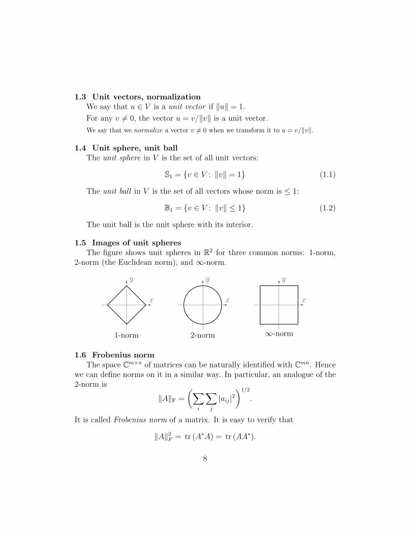
1.5 Images of unit spheresThe figure shows unit spheres in R2 for three common norms: 1-norm,

2-norm (the Euclidean norm), and ∞-norm.

x

y

1-norm

x

y

2-norm

x

y

∞-norm

1.6 Frobenius normThe space Cm×n of matrices can be naturally identified with Cmn. Hence

we can define norms on it in a similar way. In particular, an analogue of the2-norm is

‖A‖F =

(∑i

∑j

|aij|2)1/2

.

It is called Frobenius norm of a matrix. It is easy to verify that

‖A‖2F = tr (A∗A) = tr (AA∗).

8

1.7 Induced matrix normsRecall that every matrix A ∈ Fm×n defines a linear transformation Fn →

Fm. Suppose the spaces Fn and Fm are equipped with certain norms, ‖ · ‖.Then we define the induced norm (also called operator norm) of A as follows:

‖A‖ = sup‖x‖=1

‖Ax‖ = supx 6=0

‖Ax‖‖x‖

(1.3)

This norm is the maximum expansion factor, i.e., the largest factor by which the matrix

A stretches vectors x ∈ Fn.

Respectively, we obtain ‖A‖1, ‖A‖2, and ‖A‖∞, if the spaces Fn and Fmare equipped with ‖ · ‖1, ‖ · ‖2, and ‖ · ‖∞.

For students familiar with topology: The supremum in (1.3) is always attained and canbe replaced by maximum. This follows from the compactness of S1 and the continuity of‖ ·‖. For the 2-norm, this can be also proved by an algebraic argument, see Corollary 4.23.

There are norms on Cn×n that are not induced by any norm on Cn, for example

‖A‖ = maxi,j |aij | (see Exercise 1.1).

1.8 Computation of ‖A‖1, ‖A‖2, and ‖A‖∞We have simple rules for computing ‖A‖1 and ‖A‖∞:

‖A‖1 = max1≤j≤n

m∑i=1

|aij| (“maximum column sum”)

‖A‖∞ = max1≤i≤m

n∑j=1

|aij| (“maximum row sum”)

Unfortunately, there is no explicit formulas for ‖A‖2 in terms of the aij’s. Asubstantial part of this course will be devoted to the computation of ‖A‖2.

1.9 Inequalities for induced matrix normsAny induced matrix norm satisfies

‖Ax‖ ≤ ‖A‖ ‖x‖ and ‖AB‖ ≤ ‖A‖ ‖B‖.

9

1.10 Inner productsLet V be a vector space over C. An inner product on V is a complex

valued function of two vector arguments, i.e., V × V → C, denoted by 〈·, ·〉,satisfying four axioms:

1. 〈u, v〉 = 〈v, u〉 for all u, v ∈ V .

2. 〈cu, v〉 = c〈u, v〉 for all c ∈ C and u, v ∈ V .

3. 〈u+ v, w〉 = 〈u,w〉+ 〈v, w〉 for all u, v, w ∈ V .

4. 〈u, u〉 ≥ 0 for all u ∈ V , and 〈u, u〉 = 0 iff u = 0.

These axioms imply the following rules:

〈u, v + w〉 = 〈u, v〉+ 〈u,w〉 and 〈u, cv〉 = c〈u, v〉. (1.4)

i.e., the inner product is linear in the first argument (due to axioms 2 and 3)but “conjugate linear” in the second.

If V is a vector space over R, then an inner product is a real valuedfunction of two arguments, i.e., V × V → R satisfying the same axioms(except c ∈ R, and there is no need to take conjugate).

1.11 Standard inner productA standard (canonical) inner product in Cn is

〈x, y〉 =n∑i=1

xiyi = y∗x.

A standard (canonical) inner product in Rn is

〈x, y〉 =n∑i=1

xiyi = yTx.

A standard inner product in C([a, b]), the space of complex-valued continuousfunctions, is:

〈f, g〉 =

∫ b

a

f(x) g(x) dx

For real-valued functions, we can replace g(x) with g(x).

10

1.12 Cauchy-Schwarz inequalityLet V be an inner product space. Then for any two vectors u, v ∈ V

|〈u, v〉| ≤ 〈u, u〉1/2〈v, v〉1/2 (1.5)

The equality holds if and only if u and v are linearly dependent, i.e.,

|〈u, v〉| = 〈u, u〉1/2〈v, v〉1/2 ⇐⇒ au+ bv = 0 (1.6)

for some scalars a, b of which at least one is different from zero.

Proof. The easy case is where v = 0. Then 〈u, v〉 = 0 and 〈v, v〉 = 0, so bothsides of (1.5) are zero, hence the claim is trivial.

We now turn to the difficult case: v 6= 0. Consider the function

f(z) = 〈u− zv, u− zv〉= 〈u, u〉 − z〈v, u〉 − z〈u, v〉+ |z|2〈v, v〉

of a complex variable z. Let z = reiθ and 〈u, v〉 = seiϕ be the polar forms ofthe complex numbers z and 〈u, v〉, respectively. We fix θ = ϕ and note that

z〈v, u〉 = reiϕse−iϕ = rs

andz〈u, v〉 = re−iϕseiϕ = rs.

We assume that r varies from −∞ to ∞, then

0 ≤ f(z) = 〈u, u〉 − 2sr + r2〈v, v〉 (1.7)

Since this holds for all r ∈ R, the discriminant of the above quadratic poly-nomial has to be ≤ 0, i.e.

s2 − 〈u, u〉〈v, v〉 ≤ 0. (1.8)

This proves the inequality (1.5).The equality in (1.5) means the equality in (1.8), because s = |〈u, v〉|. The

equality in (1.8) means that the discriminant of the quadratic polynomial in(1.7) is zero, hence that polynomial assumes a zero value, i.e.,

f(z) = 〈u− zv, u− zv〉 = 0

for some z ∈ C. This, in turn, means u − zv = 0, thus u = zv for somez ∈ C, i.e., u and v are linearly dependent, as claimed. �

11

1.13 Induced normsIf V is an inner product vector space, then

‖v‖ = 〈v, v〉1/2 (1.9)

defines a norm on V (all the axioms can be verified by direct inspection,except the triangle inequality is proved by Cauchy-Schwarz inequality 1.12).

1.14 Polarization identitySome norms are induced by inner products, others are not. The 2-norm in

Rn and in Cn (defined in Sect. 1.2) is induced by the standard inner productin those spaces (as defined in Sect. 1.11).

In vector spaces over R, if a norm ‖ · ‖ is induced by an inner product〈·, ·〉, then the latter can be computed by polarization identity :

〈u, v〉 = 14

(‖u+ v‖2 − ‖u− v‖2

)(1.10)

A similar but more complicated polarization identity holds in vector spaces over C.

1.15 Orthogonal vectorsTwo vectors u, v ∈ V are said to be orthogonal if 〈u, v〉 = 0.

1.16 Pythagorean theoremIf two vectors u and v are orthogonal, then

‖u+ v‖2 = ‖u‖2 + ‖v‖2 (1.11)

Vectors u and v make two legs of a right triangle, and u+ v is its hypotenuse:u

u +v

v

Suppose u1, . . . , uk are mutually orthogonal, i.e., 〈ui, uj〉 = 0 for each i 6= j. Then one

can show, by induction, that ‖u1 + · · ·+ uk‖2 = ‖u1‖2 + · · ·+ ‖uk‖2.

1.17 Orthogonality and linear independenceIf nonzero vectors u1, . . . , uk are mutually orthogonal, i.e., 〈ui, uj〉 = 0 for

each i 6= j, then they are linearly independent.

Proof. Suppose a linear combination of these vectors is zero, i.e.,

c1u1 + · · ·+ ckuk = 0.

Then for every i = 1, . . . , k we have

0 = 〈0, ui〉 = 〈c1u1 + · · ·+ ckuk, ui〉 = ci〈ui, ui〉

hence ci = 0 (because 〈ui, ui〉 6= 0 for the non-zero vector ui). Thus c1 = · · · = ck = 0. �

12

1.18 Orthonormal sets of vectorsA set {u1, . . . , uk} of vectors is said to be orthonormal if all the vectors

ui are mutually orthogonal and have unit length (i.e., ‖ui‖ = 1 for all i).The orthonormality can be expressed by a single formula:

〈ui, uj〉 = δij,

where δij denotes the Kronecker delta symbol defined as follows: δij = 1 ifi = j and δij = 0 if i 6= j.

1.19 Orthonormal basis (ONB)An orthonormal set of vectors {u1, . . . , uk} that is a basis in V is called

orthonormal basis (ONB).An orthonormal set {u1, . . . , uk} is an ONB in V iff k = n = dimV .

1.20 Fourier expansionIf {u1, . . . , un} is an ONB, then for any vector v we have

v =n∑i=1

〈v, ui〉ui. (1.12)

In other words, the numbers 〈v, ui〉 (called Fourier coefficients) are the co-ordinates of the vector v in the basis {u1, . . . , un}.

1.21 Orthogonal projectionLet u, v ∈ V , and u 6= 0. The orthogonal projection of v onto u is

Pruv =〈v, u〉‖u‖2

u.

One can easily check that the vector w = v − Pruv is orthogonal to u. Thusv is the sum of two vectors: Pruv (parallel to u) and w (orthogonal to u).

u

v w

Pruv

13

1.22 Angle between vectorsIf V is a vector space over R, then for any nonzero vectors u, v ∈ V there

is a unique angle θ ∈ [0, π] such that

cos θ =〈v, u〉‖u‖ ‖v‖

. (1.13)

Indeed, by Cauchy-Schwarz inequality 1.12, the above fraction is a real number in the

interval [−1, 1]. Then recall that the function cos−1 takes [−1, 1] onto [0, π] bijectively.

We call θ the angle between u and v.Note that cos θ = 0 (i.e., θ = π/2) if and only if u and v are orthogonal. Also,

cos θ = ±1 if and only if u, v are proportional, i.e. v = cu. In that case the sign of c

coincides with the sign of cos θ.

1.23 Orthogonal projection onto a subspaceLet {u1, . . . , uk} be an orthonormal set of vectors. According to Sect. 1.17,

they are linearly independent, hence they span a k-dimensional subspaceL = span{u1, . . . , uk}. For any v ∈ V ,

PrLv =k∑i=1

〈v, ui〉ui

is the orthogonal projection of v onto L. One can easily check that the vector

w = v − PrLv

is orthogonal to all the vectors u1, . . . , uk, hence it is orthogonal to all vectorsin L. In particular, the vectors u1, . . . , uk, w are mutually orthogonal, andone can easily check that

span{u1, . . . , uk, v} = span{u1, . . . , uk, w}.

1.24 Degenerate caseIn the above construction, we have

w = 0 ⇐⇒ v ∈ span{u1, . . . , uk}.

Note: In Section 1.23, the subspace L is spanned by an orthonormal set of vectors.What if we want to project a vector v onto a subspace L that is spanned by a non-orthonormal set of vectors {v1, . . . , vk}?

14

1.25 Gram-Schmidt orthogonalizationLet {v1, . . . , vk} be a linearly independent set of vectors. They span a

k-dimensional subspace L = span{v1, . . . , vk}. Our goal is to find an or-thonormal set of vectors {u1, . . . , uk} that spans L. We will modify andadjust the vectors v1, . . . , vk, one by one.

At our first step, we define

w1 = v1 and u1 = w1/‖w1‖. (1.14)

At our second step, we define

w2 = v2 − 〈v2, u1〉u1 and u2 = w2/‖w2‖. (1.15)

Then recursively, for each p ≥ 2, we define

wp = vp −p−1∑i=1

〈vp, ui〉ui, and up = wp/‖wp‖ (1.16)

By induction on p, one can easily check that

span{v1, . . . , vp} = span{u1, . . . , up}

and wp 6= 0 (in accordance with Sect. 1.24).The above procedure is called Gram-Schmidt orthogonalization. It gives

us an orthonormal set {u1, . . . , uk} which spans the same subspace:

L = span{v1, . . . , vk} = span{u1, . . . , uk}.

1.26 Construction of ONBSuppose {v1, . . . , vn} is a basis in V . Then the Gram-Schmidt orthogo-

nalization gives us an orthonormal basis (ONB) {u1, . . . , un} in V .As a result, every finite dimensional vector space with an inner product

has an ONB. Furthermore, every set of orthonormal vectors {u1, . . . , uk} canbe extended to an ONB.

1.27 Legendre polynomials (optional)Let V = Pn(R), the space of real polynomials of degree ≤ n, with the inner product

given by 〈f, g〉 =∫ 1

0f(x)g(x) dx. Applying Gram-Schmidt orthogonalization to the basis

{1, x, . . . , xn} gives the first n+ 1 of the so called Legendre polynomials.

15

1.28 Orthogonal complementLet S ⊂ V be a subset (not necessarily a subspace). Then

S⊥ = {v ∈ V : 〈v, w〉 = 0 for all w ∈ S}

is called the orthogonal complement to S.One can easily check that S⊥ is a vector subspace of V .We also note that if W ⊂ V is a subspace of V , then (W⊥)⊥ ⊂ W .

Moreover, if V is finite dimensional, then (W⊥)⊥ = W (see Exercise 1.4).

1.29 Orthogonal direct sumIf W ⊂ V is a finite dimensional subspace of V , then V = W ⊕W⊥.

Proof. Let {u1, . . . , un} be an ONB of W (one exists according to Sect. 1.26). For anyv ∈ V define

w =

n∑i=1

〈v, ui〉ui

One can easily verify that w ∈ W and v − w ∈ W⊥. Therefore v = w + w′ where w ∈ Wand w′ ∈ W⊥. Lastly, W ∩W⊥ = {0} because any vector w ∈ W ∩W⊥ is orthogonal to

itself, i.e., 〈w,w〉 = 0, hence w = 0.

1.30 Some useful formulasLet {u1, . . . , un} be an orthonormal set (not necessarily an ONB) in V .

Then for any vector v ∈ V we have Bessel’s inequality :

‖v‖2 ≥n∑i=1

|〈v, ui〉|2. (1.17)

If {u1, . . . , un} is an ONB in V , then Bessel’s inequality turns into an equality:

‖v‖2 =n∑i=1

|〈v, ui〉|2. (1.18)

More generally, we have Parceval’s identity :

〈v, w〉 =n∑i=1

〈v, ui〉〈w, ui〉, (1.19)

which easily follows from the Fourier expansion (1.12).

16

Parceval’s identity (1.19) can be also written as follows. Suppose

v =n∑i=1

aiui and w =n∑i=1

biui,

so that (a1, . . . , an) and (b1, . . . , bn) are the coordinates of the vectors v andw, respectively, in the ONB {u1, . . . , un}. Then

〈v, w〉 =n∑i=1

aibi. (1.20)

In particular,

‖v‖2 = 〈v, v〉 =n∑i=1

aiai =n∑i=1

|ai|2. (1.21)

Exercise 1.1. Show that the norm ‖A‖ = maxi,j |aij | on the space of n×n real matricesis not induced by any vector norm in Rn. Hint: use inequalities from Section 1.7.

Exercise 1.2. Prove the Neumann lemma: if ‖A‖ < 1, then I−A is invertible. Here ‖ · ‖is a norm on the space of n× n matrices induced by a vector norm.

Exercise 1.3. Let V be an inner product space, and ‖ · ‖ denote the norm induced bythe inner product. Prove the parallelogram law

‖u+ v‖2 + ‖u− v‖2 = 2‖u‖2 + 2‖v‖2.

Based on this, show that the norms ‖ · ‖1 and ‖ · ‖∞ in C2 are not induced by any innerproducts.

Exercise 1.4. Let W ⊂ V be a subspace of an inner product space V .

(i) Prove that W ⊂ (W⊥)⊥.

(ii) If, in addition, V is finite dimensional, prove that W = (W⊥)⊥.

Exercise 1.5. Let {u1, . . . , un} be an ONB in Cn. Assuming that n is even, compute

‖u1 − u2 + u3 − · · ·+ un−1 − un‖

17

Chapter 2

Unitary Matrices

2.1 IsometriesLet V and W be two inner product spaces (both real or both complex).

An isomorphism T : V → W is called an isometry if it preserves the innerproduct, i.e.

〈Tv, Tw〉 = 〈v, w〉for all v, w ∈ V . In this case the spaces V and W are said to be isometric.

2.2 Characterization of isometries - IAn isomorphism T is an isometry iff it preserves the induced norm, i.e.,

‖Tv‖ = ‖v‖ for all vectors v ∈ V .

Proof. This follows from Polarization Identity (1.10)

2.3 Characterization of isometries - IIAn isomorphism T is an isometry iff ‖Tu‖ = ‖u‖ for all unit vectors

u ∈ V .

Proof. This easily follows from the previous section and the fact that every non-zero

vector v can be normalized by u = v/‖v‖; cf. Sect. 1.3.

2.4 Characterization of isometries - IIILet dimV < ∞. A linear transformation T : V → W is an isometry iff

there exists an ONB {u1, . . . , un} in V such that {Tu1, . . . , Tun} is an ONBin W .

Proof. If T is an isometry, then for any ONB {u1, . . . , un} in V the set {Tu1, . . . , Tun}is an ONB inW . Now suppose T takes an ONB {u1, . . . , un} in V to an ONB {Tu1, . . . , Tun}in W . Since T takes a basis in V into a basis in W , it is an isomorphism. Now for eachvector v = c1u1 + · · ·+ cnun ∈ V we have, by linearity, Tv = c1Tu1 + · · ·+ cnTun, hencev and Tv have the same coordinates in the respective ONBs. Now by Parceval’s Identity(1.21) we have

‖v‖2 = |c1|2 + · · ·+ |cn|2 = ‖Tv‖2

Thus T is an isometry according to Sect. 2.2.

18

2.5 Identification of finite-dimensional inner product spacesFinite dimensional inner product spaces V and W (over the same field)

are isometric iff dimV = dimW .(This follows from Section 2.4.)

As a result, we can make the following useful identifications:

c© All complex n-dimensional inner product spaces can be identified withCn equipped with the standard inner product 〈x, y〉 = y∗x.

R© All real n-dimensional inner product spaces can be identified with Rn

equipped with the standard inner product 〈x, y〉 = yTx.

These identifications allow us to focus on the study of the standard spaces Cn and Rn

equipped with the standard inner product.

Isometries Cn → Cn and Rn → Rn are operators that, in a standard basis{e1, . . . , en}, are given by matrices of a special type, as defined below.

2.6 Unitary and orthogonal matricesA matrix Q ∈ Cn×n is said to be unitary if Q∗Q = I, i.e., Q∗ = Q−1.A matrix Q ∈ Rn×n is said to be orthogonal if QTQ = I, i.e., QT = Q−1.

One can easily verify that

Q is unitary⇔ Q∗ is unitary⇔ QT is unitary⇔ Q is unitary.

In the real case:

Q is orthogonal⇔ QT is orthogonal.

2.7 LemmaLet A,B ∈ Fm×n be two matrices (here F = C or F = R) such that

〈Ax, y〉 = 〈Bx, y〉 for all x ∈ Fn and y ∈ Fm. Then A = B.

Proof. For any pair of canonical basis vectors ej ∈ Fn and ei ∈ Fm wehave 〈Aej, ei〉 = aij and 〈Bej, ei〉 = bij, therefore aij = bij. �

19

2.8 Matrices of isometries

c© The linear transformation of Cn defined by a matrix Q ∈ Cn×n is anisometry (preserves the standard inner product) iff Q is unitary.

R© The linear transformation of Rn defined by a matrix Q ∈ Rn×n is anisometry (preserves the standard inner product) iff Q is orthogonal.

Proof If Q is an isometry, then for any pair of vectors x, y

〈x, y〉 = 〈Qx,Qy〉 = (Qy)∗Qx = y∗Q∗Qx = 〈Q∗Qx, y〉

hence Q∗Q = I due to Lemma 2.7. Conversely: if Q∗Q = I, then

〈Qx,Qy〉 = (Qy)∗Qx = y∗Q∗Qx = y∗x = 〈x, y〉,

hence Q is an isometry. �

2.9 Group propertyIf Q1, Q2 ∈ Cn×n are unitary matrices, then so is Q1Q2.If Q ∈ Cn×n is a unitary matrix, then so is Q−1.

In terms of abstract algebra, unitary n× n matrices make a group, denoted by U(n).

Similarly, orthogonal n× n matrices make a group, denoted by O(n).

2.10 Orthogonal matrices in 2D

Q =

[0 11 0

]defines a reflection across the diagonal line y = x;

Q =

[cos θ − sin θsin θ cos θ

]is a counterclockwise rotation by angle θ.

For a complete description of 2D orthogonal matrices, see Exercises 2.3 and 2.4.

x

y

y=x

x

y

reflection rotation

20

2.11 Characterizations of unitary and orthogonal matricesA matrix Q ∈ Cn×n is unitary iff its columns make an ONB in Cn.A matrix Q ∈ Cn×n is unitary iff its rows make an ONB in Cn.

A matrix Q ∈ Rn×n is orthogonal iff its columns make an ONB in Rn.A matrix Q ∈ Rn×n is orthogonal iff its rows make an ONB in Rn.

Proof. The idea is illustrated by the following diagram:

Q∗ × Q = I = Q × Q∗

q∗1q∗2...q∗n

q1

∣∣∣∣∣∣∣∣∣ q2∣∣∣∣∣∣∣∣∣ · · ·

∣∣∣∣∣∣∣∣∣ qn =

1 0 · · · 00 1 · · · 0...

.... . .

...0 0 · · · 1

=

q1q2...qn

q∗1

∣∣∣∣∣∣∣∣∣ q∗2

∣∣∣∣∣∣∣∣∣ · · ·∣∣∣∣∣∣∣∣∣ q∗n

Here qi denotes the ith column of Q and qi denotes the ith row of Q.

The proof is now a direct inspection. �

2.12 Determinant of unitary matricesIf Q is unitary/orthogonal, then |detQ| = 1.

Proof. We have

1 = det I = detQ∗Q = detQ∗ · detQ = detQ · detQ = | detQ|2.

If Q is a real orthogonal matrix, then detA = ±1. Orthogonal n × n matrices with

determinant 1 make a subgroup of O(n), denoted by SO(n).

2.13 Eigenvalues of unitary matricesIf λ is an eigenvalue of a unitary/orthogonal matrix, then |λ| = 1.

Proof. If Qx = λx for some x 6= 0, then

〈x, x〉 = 〈Qx,Qx〉 = 〈λx, λx〉 = λλ〈x, x〉 = |λ|2〈x, x〉;

therefore |λ|2 = 1. �

Note: orthogonal matrices Q ∈ Rn×n may not have any real eigenvalues; see the rotation

matrix in Example 2.10. But if an orthogonal matrix has real eigenvalues, those equal ±1.

21

2.14 Invariance principle for isometriesLet T : V → V be an isometry and dimV <∞. If a subspace W ⊂ V is

invariant under T , i.e., TW ⊂ W , then so is its orthogonal complement W⊥,i.e., TW⊥ ⊂ W⊥.

Proof. The restriction of T to the invariant subspace W is an operator onW . It is an isometry of W , hence it is a bijection W → W , i.e.,

∀w ∈ W ∃w′ ∈ W : Tw′ = w.

Now, if v ∈ W⊥, then

∀w ∈ W : 〈w, Tv〉 = 〈Tw′, T v〉 = 〈w′, v〉 = 0,

hence Tv ∈ W⊥. This implies TW⊥ ⊂ W⊥. �

2.15 Orthogonal decomposition for complex isometriesFor any isometry T of a finite dimensional complex space V there is an

ONB of V consisting of eigenvectors of T .

Proof. Recall that eigenvalues always exist for operators on complex vectorspaces (Sect. 0.10). Let λ1 be an eigenvalue of T with an eigenvector x1 6= 0.Then W1 = span{x1} is a one-dimensional subspace invariant under T . BySection 2.14, the (n−1)-dimensional subspace W⊥

1 is also invariant under T .The restriction of T to W⊥

1 is an operator on W⊥, which is an isometry.Let λ2 be an eigenvalue of the operator T : W⊥

1 → W⊥1 , with an eigenvec-

tor x2 ∈ W⊥1 . Then W2 = span{x2} is a one-dimensional subspace of W⊥

1

invariant under T .Since both W1 and W2 are invariant under T , we have that W1 ⊕W2 is

a two-dimensional subspace of V invariant under T . By Section 2.14, the(n − 2)-dimensional subspace (W1 ⊕ W2)⊥ is also invariant under T . Therestriction of T to (W1 ⊕W2)⊥ is an isometry, too.

Then we continue, inductively: at each step we “split off” a one-dimensionalsubspace invariant under T and reduce the dimensionality of the remainingsubspace. Since V is finite dimensional, we eventually exhaust all the dimen-sions of V and complete the proof. �

Note: the above theorem is not true for real vector spaces. An isometry of a real vector

space may not have any eigenvectors; see again the rotation matrix in Example 2.10.

22

2.16 LemmaEvery operator T : V → V on a finite dimensional real space V has either

a one-dimensional or a two-dimensional invariant subspace W ⊂ V .

Proof. Let T be represented by a matrix A ∈ Rn×n in some basis. If Ahas a real eigenvalue, then Ax = λx with some x 6= 0, and we get a one-dimensional invariant subspace span{x}. If A has no real eigenvalues, thenthe matrix A, treated as a complex matrix (cf. Sect. 0.10), has a complexeigenvalue λ = a+ ib, with a, b ∈ R and i =

√−1, and a complex eigenvector

x+ iy, with x, y ∈ Rn. The equation

A(x+ iy) = (a+ ib)(x+ iy) = (ax− by) + (bx+ ay)i

can be written as

Ax = ax− byAy = bx+ ay

This implies that the subspace span{x, y} is invariant. �

Note: The above subspace span{x, y} is two-dimensional, unless x and y are linearly

dependent. With some extra effort, one can verify that x and y can be linearly dependent

only if b = 0, i.e. λ ∈ R.

2.17 Orthogonal decomposition for real isometriesLet T : V → V be an isometry of a finite dimensional real space V . Then

V = V1⊕· · ·⊕Vp for some p ≤ n, where Vi are mutually orthogonal subspaces,each Vi is T -invariant, and either dimVi = 1 or dimVi = 2.

Proof. Use induction on dimV and apply Sections 2.14 and 2.16. �

Note: the restriction of the operator T to each two-dimensional invariantsubspace Vi is simply a rotation by some angle (as in Example 2.10); thisfollows from Exercises 2.3 and 2.4.

Recall that two n × n matrices A and B are similar (usually denotedby A ∼ B) if there exists an invertible matrix X such that B = X−1AX.Two matrices are similar if they represent the same linear operator on ann-dimensional space, but under two different bases. In that case X is thechange of basis matrix.

23

2.18 Unitary and orthogonal equivalence

c© Two complex matrices A,B ∈ Cn×n are said to be unitary equivalentif B = P−1AP for some unitary matrix P . This can be also written asB = P ∗AP (because P−1 = P ∗).

R© Two real matrices A,B ∈ Rn×n are said to be orthogonally equivalentif B = P−1AP for some orthogonal matrix P . This can be also writtenas B = P TAP (because P−1 = P T ).

Two complex/real matrices are unitary/orthogonally equivalent if theyrepresent the same linear operator on a complex/real n-dimensional innerproduct space under two different orthonormal bases (ONBs). Then P isthe change of basis matrix, which must be unitary/orthogonal, because itchanges an ONB to another ONB (cf. Sect. 2.4).

In this course we mostly deal with ONBs, thus unitary/orthogonal equiv-alence will play the same major role as similarity plays in Linear Algebra.In particular, for any type of matrices we will try to find simplest matriceswhich are unitary/orthogonal equivalent to matrices of the given type.

2.19 Unitary matrices in their simples formAny unitary matrix Q ∈ Cn×n is unitary equivalent to a diagonal matrix

D = diag{d1, . . . , dn}, whose diagonal entries belong to the unit circle, i.e.|di| = 1 for 1 ≤ i ≤ n.

Proof. This readily follows from Section 2.15.

2.20 Orthogonal matrices in their simples formAny orthogonal matrix Q ∈ Rn×n is orthogonally equivalent to a block-

diagonal matrix

B =

R11 0 · · · 00 R22 · · · 0...

.... . .

...0 0 · · · Rmm

where Rii are 1× 1 and 2× 2 diagonal blocks. Furthermore, each 1× 1 blockis either Rii = +1 or Rii = −1, and each 2× 2 block is a rotation matrix

Rii =

[cos θi − sin θisin θi cos θi

]Proof. This readily follows from Section 2.17.

24

Exercise 2.1. Let A ∈ Cm×n. Show that

‖UA‖2 = ‖AV ‖2 = ‖A‖2

for any unitary matrices U ∈ Cm×m and V ∈ Cn×n.

Exercise 2.2. Let A ∈ Cm×n. Show that

‖UA‖F = ‖AV ‖F = ‖A‖F

for any unitary matrices U ∈ Cm×m and V ∈ Cn×n. Here ‖ · ‖F stands for the Frobeniusnorm.

Exercise 2.3. Let Q be a real orthogonal 2× 2 matrix and detQ = 1.Show that

Q =

[cos θ − sin θsin θ cos θ

]for some θ ∈ [0, 2π).

In geometric terms, Q represents a rotation of R2 by angle θ.

Exercise 2.4. Let Q be a real orthogonal 2× 2 matrix and detQ = −1.Show that

Q =

[cos θ sin θsin θ − cos θ

]for some θ ∈ [0, 2π).Also prove that λ1 = 1 and λ2 = −1 are the eigenvalues of Q.

In geometric terms, Q represents a reflection of R2 across the line spanned by theeigenvector corresponding to λ1 = 1.

25

Chapter 3

Hermitian Matrices

Beginning with this chapter, we will always deal with finite dimensional inner productspaces (unless stated otherwise). Recall that all such spaces can be identified with Cn orRn equipped with the standard inner product (Sect. 2.5). Thus we will mostly deal withthese standard spaces.

3.1 Adjoint matricesRecall that every complex matrix A ∈ Cm×n defines a linear transfor-

mation Cn → Cm. Its conjugate transpose A∗ ∈ Cn×m defines a lineartransformation Cm → Cn, i.e., Cn CmA

A∗

Furthermore, for any x ∈ Cn and y ∈ Cm we have

〈Ax, y〉 = y∗Ax = (A∗y)∗x = 〈x,A∗y〉

Likewise, 〈y, Ax〉 = 〈A∗y, x〉. In plain words, A can be moved from oneargument of the inner product to the other, but it must be changed to A∗.

Likewise, every real matrix A ∈ Rm×n defines a linear transformationRn → Rm. Its transpose AT ∈ Rn×m defines a linear transformation Rm →Rn. Furthermore, for any x ∈ Rn and y ∈ Rm we have

〈Ax, y〉 = yTAx = (ATy)Tx = 〈x,ATy〉

Thus in the real case, too, A can be moved from one argument of the innerproduct to the other, but it must be changed to A∗ = AT .

3.2 Adjoint transformationsMore generally, for any linear transformation T : V → W of two inner

product vector spaces V and W (both real or both complex) there exists aunique linear transformation T ∗ : W → V such that ∀v ∈ V, ∀w ∈ W

〈Tv, w〉 = 〈v, T ∗w〉.

T ∗ is often called the adjoint of T .

26

T ∗ generalizes the conjugate transpose of a matrix.

The existence and uniqueness of T ∗ can be proved by a general argument, avoidingidentification of the spaces V and W with Cn or Rn. The argument is outlined below, inSections 3.3 to 3.6. (This part of the course can be skipped.)

3.3 Riesz representation theoremLet f ∈ V ∗, i.e., let f be a linear functional on V . Then there is a unique vector u ∈ V

such thatf(v) = 〈v, u〉 ∀v ∈ V

Proof. Let B = {u1, . . . , un} be an ONB in V . Then for any v =∑ciui we have

f(v) =∑cif(ui) by linearity. Also, for any u =

∑diui we have 〈v, u〉 =

∑cidi. Hence,

the vector u =∑f(ui)ui will suffice. To prove the uniqueness of u, assume 〈v, u〉 = 〈v, u′〉

for all v ∈ V . Setting v = u− u′ gives 〈u− u′, u− u′〉 = 0, hence u = u′.

3.4 Quasi-linearityThe identity f ↔ u established in the previous theorem is “quasi-linear” in the follow-

ing sense: f1 + f2 ↔ u1 + u2 and cf ↔ cu. In the real case, it is perfectly linear, though,and hence it is an isomorphism between V ∗ and V .

3.5 RemarkIf dimV = ∞, then Theorem 3.3 fails. Consider, for example, V = C[0, 1] (real

functions) with the inner product 〈F,G〉 =∫ 1

0F (x)G(x) dx. Pick a point t ∈ [0, 1]. Let

f ∈ V ∗ be a linear functional defined by f(F ) = F (t). It does not correspond to any G ∈ Vso that f(F ) = 〈F,G〉. In fact, the lack of such functions G has led mathematicians tothe concept of delta-functions: a delta-function δt(x) is “defined” by three requirements:

δt(x) ≡ 0 for all x 6= t, δt(t) =∞ and∫ 1

0F (x)δt(x) dx = F (t) for every F ∈ C[0, 1].

3.6 Existence and uniqueness of adjoint transformationLet T : V →W be a linear transformation. Then there is a unique linear transforma-

tion T ∗ : W → V such that ∀v ∈ V and ∀w ∈W

〈Tv,w〉 = 〈v, T ∗w〉.

Proof. Let w ∈ W . Then f(v) : = 〈Tv,w〉 defines a linear functional f ∈ V ∗. By the

Riesz representation theorem, there is a unique v′ ∈ V such that f(v) = 〈v, v′〉. Then we

define T ∗ by setting T ∗w = v′. The linearity of T ∗ is a routine check. Note that in the

complex case the conjugating bar appears twice and thus cancels out. The uniqueness of

T ∗ is obvious. �

We now return to the main line of our course.

27

3.7 Relation between KerT ∗ and RangeTLet T : V → W be a linear transformation. Then

KerT ∗ = (RangeT )⊥

Proof. Suppose y ∈ KerT ∗, i.e., T ∗y = 0. Then for every x ∈ V

0 = 〈x, 0〉 = 〈x, T ∗y〉 = 〈Tx, y〉.

Thus y is orthogonal to all vectors Tx, x ∈ V , hence y ∈ (RangeT )⊥.Conversely, if y ∈ (RangeT )⊥, then y is orthogonal to all vectors Tx, x ∈ V , hence

0 = 〈Tx, y〉 = 〈x, T ∗y〉

for all x ∈ V . In particular, we can put x = T ∗y and see that 〈T ∗y, T ∗y〉 = 0, hence

T ∗y = 0, i.e., y ∈ KerT ∗. �

Next we will assume that V = W , in which case T is an operator.

3.8 Selfadjoint operators and matricesA linear operator T : V → V is said to be selfadjoint if T ∗ = T .A square matrix A is said to be selfadjoint if A∗ = A.

In the real case, this is equivalent to AT = A, i.e., A is a symmetric matrix.In the complex case, selfadjoint matrices are called Hermitian matrices.

3.9 ExamplesThe matrix [ 1 3

3 2 ] is symmetric. The matrix[

1 3+i3−i 2

]is Hermitian.

The matrices[

1 3+i3+i 2

]and

[1+i 3+i3−i 2

]are not Hermitian (why?).

Note: the diagonal components of a Hermitian matrix must be real numbers!

3.10 Hermitian property under unitary equivalence

c© If A is a complex Hermitian matrix unitary equivalent to B, then B isalso a complex Hermitian matrix.

R© If A is a real symmetric matrix orthogonally equivalent to B, then Bis also a real symmetric matrix.

Proof. If A∗ = A and B = P ∗AP , then B∗ = P ∗A∗P = P ∗AP = B. �

28

3.11 Invariance principle for selfadjoint operatorsLet T be a selfadjoint operator and a subspace W be T -invariant, i.e.,

TW ⊂ W . Then W⊥ is also T -invariant, i.e., TW⊥ ⊂ W⊥.

Proof. If v ∈W⊥, then for any w ∈W we have 〈Tv,w〉 = 〈v, Tw〉 = 0, so Tv ∈W⊥.

3.12 Spectral TheoremLet T : V → V be a selfadjoint operator. Then there is an ONB consisting

of eigenvectors of T , and all the eigenvalues of T are real numbers.

Proof. First let V be a complex space. Then we apply Principle 3.11 toconstruct an ONB of eigenvectors, exactly as we did in Section 2.15.

Now T is represented in the canonical basis {e1, . . . , en} by a Hermitianmatrix A. In the (just constructed) ONB of eigenvectors, T is represented bya diagonal matrix D = diag{d1, . . . , dn}, and d1, . . . , dn are the eigenvaluesof T . Since A and D are unitary equivalent, D must be Hermitian, too (by3.10). Hence the diagonal components d1, . . . , dn of D are real numbers. Thiscompletes the proof of Spectral Theorem for complex spaces.

Before we proceed to real spaces, we need to record a useful fact aboutcomplex Hermitian matrices. Every Hermitian matrix A ∈ Cn×n definesa selfadjoint operator on Cn. As we just proved, there exists an ONB ofeigenvectors. Hence A is unitary equivalent to a diagonal matrix D =diag{d1, . . . , dn}. Since D is Hermitian, its diagonal entries d1, . . . , dn arereal numbers. Therefore

Every Hermitian matrix has only real eigenvalues (3.1)

Now let V be a real space. In the canonical basis {e1, . . . , en}, the self-adjoint operator T : V → V is represented by a real symmetric matrix A.The latter, considered as a complex matrix, is Hermitian, thus it has only realeigenvalues (see above). Hence the construction of an ONB of eigenvectors,as done in Section 2.15, works again. The proof is now complete. �

Note: For every real symmetric matrix A, the characteristic polynomial is CA(x) =∏i(x− λi), where all λi’s are real numbers.

29

3.13 Characterization of Hermitian matrices

c© A complex matrix is Hermitian iff it is unitary equivalent to a diagonalmatrix with real diagonal entries.

R© A real matrix is symmetric iff it is orthogonally equivalent to a diagonalmatrix (whose entries are automatically real).

More generally: if an operator T : V → V has an ONB of eigenvectors, andall its eigenvalues are real numbers, then T is self-adjoint.

3.14 Eigendecomposition for Hermitian matricesLet A = QDQ∗, where Q is a unitary matrix and D is a diagonal matrix.

Denote by qi the ith column of Q and by di the ith diagonal entry of D.Then

Aqi = diqi, 1 ≤ i ≤ n

i.e. the columns of Q are eigenvectors of A whose eigenvalues are the corre-sponding diagonal components of D (cf. Section 0.11).

3.15 Inverse of a selfadjoint operator(a) If an operator T is selfadjoint and invertible, then so is T−1.(b) If a matrix A is selfadjoint and nonsingular, then so is A−1.

Proof. (a) By Spectral Theorem 3.12, there is an ONB {u1, . . . , un} consistingof eigenvectors of T , and the eigenvalues λ1, . . . , λn of T are real numbers.Since T is invertible, λi 6= 0 for all i = 1, . . . , n. Now

Tui = λiui =⇒ T−1ui = λ−1i ui

hence T−1 has the same eigenvectors {u1, . . . , un}, and its eigenvalues are thereciprocals of those of T , so they are real numbers, too. Therefore, T−1 isselfadjoint.

(b) If A is selfadjoint, then A = P ∗DP with a unitary matrix P and adiagonal matrix D = diag{d1, . . . , dn} with real diagonal entries. Now

A−1 = P−1D−1(P ∗)−1 = P ∗D−1P

where D−1 = diag{d−11 , . . . , d−1

n } is also a diagonal matrix with real diagonalentries. Therefore A−1 is selfadjoint. �

30

3.16 ProjectionsLet V = W1 ⊕W2, i.e., suppose our vector space V is a direct sum of

two subspaces. Recall that for each v ∈ V there is a unique decompositionv = w1 + w2 with w1 ∈ W1 and w2 ∈ W2.

The operator P : V → V defined by

Pv = P (w1 + w2) = w2

is called projection (or projector) of V on W2 along W1.Note that

KerP = W1 and RangeP = W2.

Also note that P 2 = P .

vw1

w2

W1

W2

KerP

RangeP

3.17 Projections (alternative definition)An operator P : V → V is a projection iff P 2 = P .

Proof. P 2 = P implies that for every v ∈ V we have P (v − Pv) = 0, so

w1 : = v − Pv ∈ KerP

Denoting w2 = Pv we get v = w1 +w2 with w1 ∈KerP and w2 ∈ RangeP . Furthermore,

Pv = Pw1 + Pw2 = 0 + P (Pv) = P 2v = Pv = w2

We also note that KerP ∩ RangeP = {0}. Indeed, for any v ∈ RangeP we have Pv = v

(as above) and for any v ∈ KerP we have Pv = 0. Thus v ∈ KerP ∩ RangeP implies

v = 0. Hence V = KerP ⊕ RangeP . �

3.18 “Complimentary” projectionsLet V = W1 ⊕ W2. There is a unique projection P1 on W1 along W2

and a unique projection P2 on W2 along W1. They “complement” each otheradding up to the identity:

P1 + P2 = I.

31

3.19 Orthogonal projectionsLet V be an inner product vector space (not necessarily finite dimen-

sional) and W ⊂ V a finite dimensional subspace. Then the projection onW along W⊥ is called orthogonal projection on W .

The assumption dimW <∞ is made to ensure that V = W ⊕W⊥ (cf. Sect. 1.29).

3.20 Characterization of orthogonal projectionsLet P be a projection. Then P is an orthogonal projection if and only if

P is selfadjoint.

Proof. Let P be a projection on W2 along W1, and V = W1⊕W2. For any vectors v, w ∈ Vwe have v = v1 + v2 and w = w1 + w2 with some vi, wi ∈Wi, i = 1, 2.

Now, if P is an orthogonal projection, then

〈Pv,w〉 = 〈v2, w〉 = 〈v2, w2〉 = 〈v, w2〉 = 〈v, Pw〉.

If P is not an orthogonal projection, then there are v1 ∈ W1 and w2 ∈ W2 so that

〈v1, w2〉 6= 0. Then 〈v1, Pw2〉 6= 0 = 〈Pv1, w2〉. �

Exercise 3.1. Let V be an inner product space and W ⊂ V a finite dimensional subspacewith ONB {u1, . . . , un}. For every x ∈ V define

P (x) =

n∑i=1

〈x, ui〉ui

(i) Prove that x− P (x) ∈W⊥, hence P is the orthogonal projection onto W .(ii) Prove that ‖x− P (x)‖ ≤ ‖x− z‖ for every z ∈ W , and that if ‖x− P (x)‖ = ‖x− z‖for some z ∈W , then z = P (x).

Exercise 3.2. (JPE, May 1999) Let P ∈ Cn×n be a projector. Show that ‖P‖2 ≥ 1 withequality if and only if P is an orthogonal projector.

32

Chapter 4

Positive Definite Matrices

Recall that an inner product 〈·, ·〉 is a complex-valued function of twovector arguments, cf. Section 1.10. It is linear in the first argument and“conjugate linear” in the second.

In the space Cn, any function f : Cn×Cn → C with the last two propertiescan be defined by

f(x, y) = 〈Ax, y〉 = y∗Ax,

where A ∈ Cn×n is a matrix. Then f(x, y) automatically satisfies axioms 2and 3 of the inner product (Sect. 1.10), as well as the rules (1.4).

But axiom 1 of the inner product (Sect. 1.10) may not hold for any suchf(x, y). It holds if and only if

〈Ax, y〉 = f(x, y) = f(y, x) = 〈Ay, x〉 = 〈x,Ay〉 = 〈A∗x, y〉,

i.e., iff A = A∗, which means that A must be a Hermitian matrix.Furthermore, if we want f(x, y) satisfy all the axioms of the inner product,

then we need to ensure the last axiom 4:

f(x, x) = 〈Ax, x〉 > 0 ∀x 6= 0.

4.1 Positive definite matricesA matrix A is said to be positive definite if it is Hermitian and

〈Ax, x〉 = x∗Ax > 0 ∀x 6= 0.

In the real case, a matrix A is positive definite if it is symmetric and

〈Ax, x〉 = xTAx > 0 ∀x 6= 0.

If we replace “> 0” with “≥ 0” in the above formulas, we get the definitionof positive semi-definite3 matrices.

3Perhaps, a more natural term would be “non-negative definite”, but we will use theofficial name positive semi-definite.

33

Symmetric positive definite matrices play important role in optimization theory (the

minimum of a function of several variables corresponds to a critical point where the ma-

trix of second order partial derivatives is positive definite) and probability theory (the

covariance matrix of a random vector is symmetric positive definite).

Interestingly, the condition 〈Ax, x〉 > 0 for all x ∈ Cn implies that the matrixA is Hermitian, and therefore positive definite. We will prove this in Sections 4.2and 4.3. (It is just a curious fact, with little importance, so the next two sectionscan be skipped.)

4.2 LemmaLet A,B be complex matrices. If 〈Ax, x〉 = 〈Bx, x〉 for all x ∈ Cn, then A = B.

(Proof: see exercises.)

Note: this lemma holds only in complex spaces, it fails in real spaces (see exercises).

4.3 Sufficient condition for positive definitenessIf A is a complex matrix such that 〈Ax, x〉 ∈ R for all x ∈ Cn, then A is

Hermitian. In particular, if 〈Ax, x〉 > 0 for all non-zero vectors x ∈ Cn, then A ispositive definite.

Proof. We have〈Ax, x〉 = 〈Ax, x〉 = 〈x,Ax〉 = 〈A∗x, x〉,

hence A = A∗ by Lemma 4.2. Now the condition 〈Ax, x〉 > 0 for all x 6= 0 implies

that A is positive definite. �

Next we define positive definite and positive semi-definite operators in general spaces in a moreabstract way; see Sections 4.4–4.11 below. (These sections can be skipped in class and assigned to moreadvanced students as a reading project.)

4.4 Bilinear formsA bilinear form on a complex vector space V is a complex-valued function of two vector arguments,

i.e., f : V × V → C such that

f(u1 + u2, v) = f(u1, v) + f(u2, v)

f(cu, v) = cf(u, v)

f(u, v1 + v2) = f(u, v1) + f(u, v2)

f(u, cv) = cf(u, v)

for all vectors u, v, ui, vi ∈ V and scalars c ∈ C. In other words, f must be linear in the first argumentand “conjugate linear” in the second.

A bilinear form on a real vector space V is a mapping f : V ×V → R that satisfies the same properties,except c is a real scalar, i.e., c = c.

34

4.5 Representation of bilinear formsLet V be a finite dimensional inner product space. Then for every bilinear form f on V there is a

unique linear operator T : V → V such that

f(u, v) = 〈Tu, v〉 ∀u, v ∈ V

Proof. For every v ∈ V the function g(u) = f(u, v) is linear in u, so by Riesz Representation Theorem 3.3there is a vector w ∈ V such that f(u, v) = 〈u,w〉. Define a map S : V → V by Sv = w. It is then aroutine check that S is linear. Setting T = S∗ proves the existence. The uniqueness is obvious. �

4.6 Corollary

c© Every bilinear form on Cn can be represented by f(x, y) = 〈Ax, y〉 with some A ∈ Cn×n.

R© Every bilinear form on Rn can be represented by f(x, y) = 〈Ax, y〉 with some A ∈ Rn×n.

Bilinear forms generalize the notion of inner product in abstract spaces. In order for a bilinear form tobecome an inner product, though, it needs two additional properties: conjugate symmetry f(x, y) = f(y, x)and the positivity f(x, x) > 0 for all x 6= 0.

4.7 Hermitian/symmetric forms

A bilinear form f on a complex space V is Hermitian if f(u, v) = f(v, u) ∀u, v ∈ V .A bilinear form f on a real space V is symmetric if f(u, v) = f(v, u) ∀u, v ∈ V .

4.8 Quadratic formsFor a Hermitian bilinear form f , the function q : V → R defined by q(u) = f(u, u) is called the

quadratic form associated with f . Note that q(u) ∈ R even in the complex case, because f(u, u) = f(u, u).

4.9 TheoremA linear operator T : V → V is selfadjoint if and only if the bilinear form f(u, v) = 〈Tu, v〉 is

Hermitian (in the real case, symmetric).

Proof. If T is selfadjoint, then f(u, v) = 〈Tu, v〉 = 〈u, Tv〉 = 〈Tv, u〉 = f(v, u). If f is Hermitian, then

〈u, Tv〉 = 〈Tv, u〉 = f(v, u) = f(u, v) = 〈Tu, v〉 = 〈u, T ∗v〉, therefore T = T ∗. �

Thus, Hermitian bilinear forms on Cn are defined by Hermitian matrices.

4.10 Positive definite forms and operatorsA Hermitian (symmetric) bilinear form f on a vector space V is said to be positive definite if f(u, u) >

0 for all u 6= 0. A selfadjoint operator T : V → V is said to be positive definite if 〈Tu, u〉 > 0 for all u 6= 0.

If we replace “> 0” with “≥ 0” in the above formulas, we get the definition of positive semi-definitebilinear forms and operators.

4.11 TheoremThe following are equivalent:

(a) a bilinear form f(u, v) is an inner product.

(b) f(u, v) = 〈Tu, v〉, where T is a positive definite operator.

We now return to the main line of our course.

35

Special note: The rest of Chapter 4 and the entire Chapter 5 are extremely important.The instructor should go slow, cover every minor detail, and not hesitate spending extratime explaining things. The students are advised to attend classes, closely follow thelectures, and do their best to fully grasp the material. Covering this part of the coursewell will allow the class to move faster through subsequent chapters. On the other hand,failure to fully understand this part of the course will cause major troubles later, and itmight be virtually impossible to learn some of the subsequent topics.

Let A ∈ Cn×n be a Hermitian matrix. By (3.1), all its eigenvaluesλ1, . . . , λn are real numbers, hence they can be ordered. In particular, wecan define

λmin = min1≤i≤n

λi and λmax = max1≤i≤n

λi. (4.1)

4.12 Properties of Hermitian matricesLet A ∈ Cn×n be a Hermitian matrix. Then

(a) For every vector x ∈ Cn we have

〈Ax, x〉 ∈ R. (4.2)

(b) For every vector x ∈ Cn we have

λmin‖x‖22 ≤ 〈Ax, x〉 ≤ λmax‖x‖2

2. (4.3)

(c) We have

〈Ax, x〉 = λmin‖x‖22 ⇐⇒ Ax = λminx (4.4)

and〈Ax, x〉 = λmax‖x‖2

2 ⇐⇒ Ax = λmaxx (4.5)

Part (c) implies that the left and right inequalities in (4.3) cannot be im-proved – they turn into equalities for certain nonzero vectors x.

Proof. By Spectral Theorem 3.12, there is an ONB {u1, . . . , un} of eigenvec-tors of A, corresponding to the eigenvalues λ1, . . . , λn. Then for any vectorx =

∑ciui we have Ax =

∑λiciui. Due to (1.20), we have

〈Ax, x〉 = λ1c1c1 + · · ·+ λncncn

= λ1|c1|2 + · · ·+ λn|cn|2.

36

Since λi ∈ R, we conclude that 〈Ax, x〉 ∈ R thus proving part (a). Next,

〈Ax, x〉 ≥ λmin

(|c1|2 + · · ·+ |cn|2

)= λmin‖x‖2

2,

where we used (1.21). We also see that

〈Ax, x〉 − λmin‖x‖22 =

n∑i=1

|ci|2(λi − λmin),

where all the terms are nonnegative because λi ≥ λmin. Thus, the left in-equality in (4.3) turns into an equality if and only if ci = 0 for all i’s suchthat λi > λmin. This means exactly that x is an eigenvector corresponding tothe smallest eigenvalue λmin. The left inequality in (4.3) and the claim (4.4)are now proved.

Similarly,

〈Ax, x〉 ≤ λmax

(|c1|2 + · · ·+ |cn|2

)= λmax‖x‖2

2

and

λmax‖x‖22 − 〈Ax, x〉 =

n∑i=1

|ci|2(λmax − λi).

Thus, the right inequality in (4.3) turns into an equality if and only if ci = 0for all i’s such that λmax > λi, which means exactly that x is an eigenvectorcorresponding to the largest eigenvalue λmax. The right inequality in (4.3)and the claim (4.5) are now proved, too. �

4.13 Eigenvalues of positive definite matricesLet A ∈ Cn×n be a Hermitian matrix. It is positive definite iff all its

eigenvalues are positive.Similarly, a Hermitian matrix A ∈ Cn×n is positive semi-definite iff all its

eigenvalues are nonnegative.

Proof. This readily follows from Section 4.12. �

4.14 Inverse of a positive definite matrixIf a matrix A is positive definite, then so is A−1.

37

4.15 Characterization of positive definite matricesA matrix A ∈ Cn×n is positive definite iff there is a nonsingular matrix

B such that A = B∗B.

Proof. “⇐” If A = B∗B, then A∗ = B∗(B∗)∗ = A, so A is Hermitian. Now

〈Ax, x〉 = 〈Bx,Bx〉 > 0 ∀x 6= 0,

so A is positive definite (note that x 6= 0 implies Bx 6= 0, because B isnonsingular).

“⇒” According to Sections 3.13 and 4.13, A = P−1DP , where D =diag {d1, . . . , dn} is a diagonal matrix with positive diagonal entries di > 0,and P is a unitary matrix. We construct a new diagonal matrix

D1/2 = diag {√d1, . . . ,

√dn}.

Now A = B2 where B = P−1D1/2P . Lastly we note that B is Hermitian,due to Section 3.13, hence A = B∗B. �

4.16 Characterization of positive semi-definite matricesA matrix A ∈ Cn×n is positive semi-definite if and only if there is a matrix

B (not necessarily nonsingular) such that A = B∗B.

The proof is similar to the above, so we omit it.

4.17 Full rank and rank deficient matricesA matrix A ∈ Cm×n is said to have full rank if

rankA = min{m,n}

Otherwise, A is said to be rank deficient.

4.18 Products A∗A and AA∗

Let A be a rectangular m× n matrix. Then the matrices A∗A and AA∗

are Hermitian and positive semi-definite. If m 6= n and A has full rank, thenthe smaller of the two matrices A∗A and AA∗ is positive definite.

Proof. First we verify the Hermitian property:

(A∗A)∗ = A∗(A∗)∗ = A∗A

38

and similarly (AA∗)∗ = AA∗. Next we verify positive semidefiniteness:

〈A∗Ax, x〉 = 〈Ax,Ax〉 ≥ 0

for any x ∈ Cn and similarly

〈AA∗y, y〉 = 〈A∗y, A∗y〉 ≥ 0

for any y ∈ Cm.Now let A have full rank. If m ≥ n, then Ker(A) = {0}, hence Ax 6= 0

for any 0 6= x ∈ Cn, so that 〈A∗Ax, x〉 = 〈Ax,Ax〉 > 0, which implies thatA∗A is positive definite. If m < n, then Range(A) = Cm, hence for any0 6= y ∈ Cm there is 0 6= x ∈ Cn such that y = Ax. Therefore

〈A∗y, x〉 = 〈y, Ax〉 = 〈y, y〉 > 0

which implies A∗y 6= 0. Therefore

〈AA∗y, y〉 = 〈A∗y, A∗y〉 > 0

which implies that AA∗ is positive definite. �

4.19 Spectral radiusLet A ∈ Cn×n be a square matrix and λ1, . . . , λn its eigenvalues. Then

ρA = max1≤i≤n

|λi|

is called the spectral radius of A. It is the radius of the smallest disk {|z| ≤ r}in the complex plane that contains all the eigenvalues of A.

Note: if A is a Hermitian matrix, then

ρA = max{|λmax|, |λmin|}

in the notation of (4.1).

39

4.20 Spectral radius for Hermitian matricesIf A ∈ Cn×n is a Hermitian matrix, then

‖A‖2 = ρA.

Proof. We use the notation of the proof in Section 4.12:

‖Ax‖22 = 〈Ax,Ax〉 = λ2

1|c1|2 + · · ·+ λ2n|cn|2

≤[

max1≤i≤n

λ2i

] n∑j=1

|cj|2 = ρ2A ‖x‖2

2.

Taking the square root and assuming x 6= 0 we get

‖Ax‖2/‖x‖2 ≤ ρA.

Now there exists k ∈ [1, n] such that |λk| = ρA. Let x = uk, i.e., x is aneigenvector corresponding to λk. Then ck = 1 and ci = 0 for all i 6= k.Therefore

‖Ax‖22 = λ2

k = ρ2A.

Combining the above estimates gives us

‖A‖2 = maxx 6=0‖Ax‖2/‖x‖2 = ρA

as desired. �

The next theorem is particularly important.

4.21 Theorem on the 2-norm of matricesFor any matrix A ∈ Cm×n we have

‖A‖22 = ‖A∗‖2

2 = ‖A∗A‖2 = ‖AA∗‖2 = λmax

where λmax denotes the largest eigenvalue of both A∗A and AA∗.

Note: This theorem gives a practical method for computing ‖A‖2 for small matrices,

where m = 2 or n = 2. In that case one of the two matrices A∗A and AA∗ is of size 2× 2,

thus its eigenvalues are the roots of a quadratic polynomial.

Proof of Theorem 4.21 is long and will be done in four steps. In the proof,‖ · ‖ will always denote the 2-norm.

40

Lemma. For every vector z ∈ Cn we have ‖z‖ = max‖y‖=1 |〈y, z〉|.Proof. Indeed, by the Cauchy-Schwarz inequality

|〈y, z〉| ≤ 〈y, y〉1/2〈z, z〉1/2 = ‖z‖

and the equality is attained whenever y is parallel to z. So we can sety = ± z

‖z‖ and achieve the maximum. �

Step 1. To prove that ‖A‖ = ‖A∗‖ we write

‖A‖ = sup‖x‖=1

‖Ax‖ = sup‖x‖=1

sup‖y‖=1

|〈y, Ax〉| = sup‖x‖=1

sup‖y‖=1

|〈A∗y, x〉|

= sup‖y‖=1

sup‖x‖=1

|〈x,A∗y〉| = sup‖y‖=1

‖A∗y‖ = ‖A∗‖.

Step 2. To prove that ‖A‖2 = ‖A∗A‖ we write

‖A∗A‖ = sup‖x‖=1

‖A∗Ax‖ = sup‖x‖=1

sup‖y‖=1

|〈y, A∗Ax〉| = sup‖x‖=1

sup‖y‖=1

|〈Ay,Ax〉|.

Then we again use the Cauchy-Schwarz inequality:

|〈Ay,Ax〉| ≤ ‖Ax‖ ‖Ay‖ ≤ ‖A‖ ‖A‖ = ‖A‖2

hence ‖A∗A‖ ≤ ‖A‖2. On the other hand,

‖A∗A‖ = sup‖x‖=1

sup‖y‖=1

|〈Ay,Ax〉| ≥ sup‖x‖=1

|〈Ax,Ax〉| = ‖A‖2.

Combining the upper and lower bounds gives us ‖A∗A‖ = ‖A‖2.

Step 3. Using an obvious symmetry we conclude that ‖A∗‖2 = ‖AA∗‖.Step 4. According to Section 4.20, we have

‖A∗A‖2 = max |λi(A∗A)|.

Recall that A∗A is a Hermitian positive semi-definite matrix, so its eigenval-ues λi(A

∗A) are real and ≥ 0, hence max |λi(A∗A)| = λmax(A∗A), the largesteigenvalue of A∗A. The same argument applies to AA∗. In particular, we seethat

λmax(A∗A) = λmax(AA∗).

This completes the proof of Theorem 4.21. �

41

4.22 Example

Let A =

[34

]∈ C2×1. For any unit vector x ∈ C1 we can write x = [eiθ],

therefore Ax =

[3eiθ

4eiθ

]and

‖Ax‖ =√|3eiθ|2 + |4eiθ|2 =

√32 + 42 = 5

which implies ‖A‖ = 5. Now let us find the norm of A∗ =[3 4

]∈ C1×2,

i.e., ‖A∗‖ = sup‖y‖=1 ‖A∗y‖. For simplicity, we will only use real unit vectors

y ∈ C2, which can be described by y =

[cosϕsinϕ

]for ϕ ∈ [0, 2π]. We have

A∗y = 3 cosϕ+4 sinϕ, thus ‖A∗y‖ = |3 cosϕ+4 sinϕ|. Finding the maximumof this function (over the interval 0 ≤ ϕ ≤ 2π) is a Calculus-I problem: themaximum is achieved at cosϕ = ±3/5 and sinϕ = ±4/5, and we get

‖A∗‖ = max‖y‖=1

‖A∗y‖ =9

5+

16

5=

25

5= 5.

We see that, indeed, ‖A‖ = ‖A∗‖. Note that A∗A = [25] ∈ C1×1, so obviously‖A∗A‖ = 25, in full agreement with Theorem 4.21.

4.23 Corollary for the 2-norm of matricesLet λmax again denote the largest eigenvalue of A∗A. Then we have

‖Ax‖2 = ‖A‖2‖x‖2 ⇐⇒ A∗Ax = λmaxx.

Hence, the supremum in Section 1.7 is attained (on the eigenvectors of A∗Acorresponding to λmax) and can be replaced by maximum. Moreover, thisimplies that the 2-norm of a real matrix is the same, whether it is computedin the complex space or in the real space.

Proof. On the one hand

‖Ax‖22 = 〈Ax,Ax〉 = 〈A∗Ax, x〉

and on the other hand‖A‖2 = λmax,

so for any vector x with ‖x‖ = 1 we have

‖Ax‖22 = ‖A‖2

2 ⇐⇒ 〈A∗Ax, x〉 = λmax,

and lastly we use Section 4.12. �

42

Exercise 4.1. Let A ∈ Cn×n satisfy A∗ = −A. Show that the matrix I −A is invertible.Then show that the matrix (I −A)−1(I +A) is unitary.

Exercise 4.2. Let A = (aij) be a complex n× n matrix. Assume that 〈Ax, x〉 = 0 for allx ∈ Cn. Prove that(a) aii = 0 for 1 ≤ i ≤ n by substituting x = ei(b) aij = 0 for i 6= j by substituting x = pei+qej then using (a) and putting p, q = ±1,±i(here i =

√−1) in various combinations.

Conclude that A = 0.

Exercise 4.3. Let A,B be complex n × n matrices such that 〈Ax, x〉 = 〈Bx, x〉 for allx ∈ Cn. Use the previous exercise to prove that A = B.

Exercise 4.4. Find a real 2× 2 matrix A 6= 0 such that 〈Ax, x〉 = 0 for all x ∈ R2. Thusfind two real 2 × 2 matrices A and B such that 〈Ax, x〉 = 〈Bx, x〉 for all x ∈ R2, butA 6= B.

Exercise 4.5. Find a real 2× 2 matrix A such that 〈Ax, x〉 > 0 for all x ∈ R2, but A isnot positive definite.

43

Chapter 5

Singular Value Decomposition

Recall that every matrix A ∈ Cm×n defines a linear transformation Cn →Cm. Let B be an ONB in Cn and B′ be ONB in Cm. Then T is representedin the bases B and B′ by the matrix U∗AV , where U ∈ Cm×m and V ∈ Cn×n

are unitary matrices. The following theorem shows that one can always findtwo bases B and B′ so that the matrix U∗AV will be diagonal. This can bewritten as U∗AV = D or equivalently, A = UDV ∗.

SVD (m > n) =

A

×

U

×0

0

DV ∗

SVD (m < n) =

A

×

U

×0

0

DV ∗

Note: D ∈ Cm×n is said to be diagonal if Dij = 0 for i 6= j. It has exactlyp = min{m,n} diagonal entries and can be denoted by D = diag{d1, . . . , dp}.

5.1 Singular value decomposition (SVD)Let A ∈ Cm×n and denote p = min{m,n}. Denote the rank of A by r

(0 ≤ r ≤ p). Then there are unitary matrices U ∈ Cm×m and V ∈ Cn×n anda real diagonal matrix D = diag{σ1, . . . , σp} ∈ Rm×n such that

A = UDV ∗ (5.1)

andσ1 ≥ · · · ≥ σr > σr+1 = · · · = σp = 0,

The matrix D is uniquely determined by A.

The matrices U and V are not unique, for every A there are many choices of U and V .

44

Proof. Observe that (5.1) is equivalent to A∗ = V DTU∗, which is an SVDfor A∗. Therefore, A has an SVD if and only if A∗ does. This allows us toassume that m ≥ n, without loss of generality.

We now fix l = m − n ≥ 0 and use induction on n (for every n ≥ 1 weautomatically take m = n+ l).

Denote σ1 = ‖A‖2. If σ1 = 0, then A is a zero matrix (aij = 0 for alli, j), and an SVD is constructed trivially: D is a zero matrix and U and Vare arbitrary unitary matrices. So let us assume that σ1 > 0.

Due to Corollary 4.23, there is a unit vector v1 ∈ Cn such that ‖Av1‖2 =‖A‖2 = σ1. Then the vector u1 = Av1/σ1 is a unit vector in Cm.

According to Section 1.26, we can extend v1 to an ONB {v1, v′2, . . . , v

′n}

in Cn and u1 to an ONB {u1, u′2, . . . , u

′m} in Cm. Let V1 denote the unitary

matrix whose columns are v1, v′2, . . . , v

′n and U1 denote the unitary matrix

whose columns are u1, u′2, . . . , u

′m. Then the product S = U∗1AV1 has the

following structure (as one can verify directly):

U∗1AV1 = S =

[σ1 w∗

0 B

](∗)

If n = 1, then S = [ σ10 ] is a diagonal matrix yielding an SVD

A = U1SV∗

1

for A. This is the basis for our induction.Suppose now n > 1, observe that

‖S‖2 = ‖S∗‖2 ≥∥∥∥∥[ σ1 0

w B∗

] [10

]∥∥∥∥2

=

∥∥∥∥[ σ1

w

]∥∥∥∥2

=√σ2

1 + w∗w.

On the other hand, the matrices U∗1 and V1 are unitary, hence we have

‖S‖2 = ‖U∗1AV1‖2 = (Exercise 2.1) = ‖A‖2 = σ1.

Comparing the above two formulas shows that w = 0. The matrix B hasdimensions (m − 1) × (n − 1), thus by our inductive assumption it has anSVD, let us denote it by B = UDV ∗. Now it can be easily verified that

A = U1

[1 0

0 U

]︸ ︷︷ ︸

U

[σ1 0

0 D

]︸ ︷︷ ︸

D

[1 0

0 V ∗

]V ∗1︸ ︷︷ ︸

V ∗

45

which gives us an SVD for A.To prove the uniqueness of D, observe that

A∗A = V DTDV ∗ and AA∗ = UDDTU∗

i.e., σ21, . . . , σ

2p are the eigenvalues of both A∗A and AA∗, hence they are

uniquely determined by A. �

Incidentally, the last part of the proof shows that the matrices A∗A andAA∗ have common non-zero eigenvalues.

Note also that the columns of U are eigenvectors of AA∗ and the columnsof V are eigenvectors of A∗A, according to Section 3.14.

5.2 Singular values and singular vectors

• The positive numbers σ1, . . . , σr are called singular values of A.

• The columns v1, . . . , vn of the matrix V (not those of V ∗) are calledright singular vectors for A.

• The columns u1, . . . , um of the matrix U are called left singular vectorsfor A.

5.3 Real SVDIf A ∈ Rm×n is a real matrix, then it has a real SVD

A = UDV T (5.2)

where U ∈ Rm×m and V ∈ Rn×n are real orthogonal matrices.

Proof is just a repetition of the proof in Section 5.1, except v1, v′2, . . . , v

′n and u1, u

′2, . . . , u

′m

must be real vectors. �

The following diagram illustrates the SVD; see also Section 5.4:

v1

v2 V ∗

e1

e2 D

σ1e1

σ2e2U

σ1u1

σ2u2

A

46

5.4 SVD analysisFor 1 ≤ i ≤ r we have

Avi = σiui, A∗ui = σivi.

We also have

KerA = span{vr+1, . . . , vn}, KerA∗ = span{ur+1, . . . , um}RangeA = span{u1, . . . , ur}, RangeA∗ = span{v1, . . . , vr}

andrankA = rankA∗ = r.

Here is a diagram illustrating the previous relations:

A A∗

v1

×σ1

−−−→ u1

×σ1

−−−→ v1

v2

×σ2

−−−→ u2

×σ2

−−−→ v2...

......

......

vr×σr−−−→ ur

×σr−−−→ vr

vr+1 → 0 ur+1 → 0...

......

...vn → 0 um → 0

5.5 Useful relations - IFor any matrix A ∈ Cm×n, an SVD for A∗ is

A∗ = V DTU∗,

hence A and A∗ have the same singular values. In particular,

‖A‖2 = ‖A∗‖2 = ‖D‖2 = ‖DT‖2 = σ1.

If A ∈ Cn×n is a square invertible matrix, then

A−1 = V D−1U∗

where D−1 = diag{σ−11 , . . . , σ−1

n }, and

‖A−1‖2 = ‖D−1‖2 = σ−1n .

If A ∈ Cn×n is a Hermitian matrix with eigenvalues λ1, . . . , λn, then itssingular values are |λ1|, . . . , |λn| (this follows from Section 3.13).

47

5.6 Computation of SVD for small matricesOne can manually compute an SVD of an m× 2 matrix as follows. First

we form the 2 × 2 matrix A∗A. Then we find its eigenvalues λ1 ≥ λ2 ≥ 0by solving the corresponding quadratic equation. (Since A∗A is a Hermitiampositive semi-definite matrix, its eigenvalues are real non-negative numbers.)Then we find the corresponding unit eigenvectors v1, v2 of the matrix A∗A.Then we compute σ1 =

√λ1, σ2 =

√λ2 and u1 = σ−1

1 Av1, u2 = σ−12 Av2.

(Recall that u1 and u2 must be unit vectors orthogonal to each other.) Lastly,ifm > 2, we extend the orthonormal set {u1, u2} to an ONB in Cm arbitrarily.

5.7 Reduced SVDLet A ∈ Cm×n with m > n. Then there is a matrix U ∈ Cm×n with

orthonormal columns, a unitary matrix V ∈ Cn×n and a square diagonalmatrix D = diag{σ1, . . . , σn} such that

A = UDV ∗. (5.3)

For m < n, the reduced SVD is similar: there exist a unitary matrix U ∈Cm×m, a matrix V ∈ Cn×m with orthonormal columns, and a square diagonalmatrix D = diag{σ1, . . . , σm} such that

A = UDV ∗, (5.4)

Proof. Suppose m > n. Then we take the (full) SVD A = UDV ∗ given by(5.1) and erase the last m− n columns of U and the bottom m− n rows ofD (consisting of zeros). For m < n, the construction is similar. �

Reduced SVD(m > n)

=

A

×

U

×0

0

D

V ∗

Reduced SVD(m < n)

=

A

×

U

×0

0

DV ∗

48

5.8 Rank-one expansionWe have the following expansion of A:

A =r∑i=1

σiuiv∗i (5.5)

Each term of this sum is an m× n matrix of rank one (Exercise 5.1).

Proof. It is enough to observe that for every vj, 1 ≤ j ≤ n,( r∑i=1

σiuiv∗i

)vj = σjuj = Avj

because v∗i vj = δij (the Kronecker delta symbol defined in Sect. 1.18). �

5.9 Useful relations - IIRecall the Frobenius norm of a matrix (Section 1.6). We have

‖A‖2F = (Exercise 2.2) = ‖D‖2

F = σ21 + · · ·+ σ2

r .

Comparing this with Section 5.5 gives

‖A‖2 ≤ ‖A‖F , (5.6)

The value of ‖A‖2F can be interpreted as the mass (or energy) of the matrix A. The mass

is conserved under multiplication by unitary matrices (Exercise 2.2), and the SVD pulls

all the mass of a matrix onto its diagonal.

For any 1 ≤ k ≤ r, let Ak denote the partial k-sum of (5.5):

Ak =k∑i=1

σiuiv∗i . (5.7)

It is easy to see that Akvi = σiui for i = 1, . . . , k and Akvi = 0 for i > k,therefore rankAk = k.

Comparing (5.7) with (5.5) we see that Ak has singular values σ1, . . . , σkand singular vectors u1, . . . , uk and v1, . . . , vk. Thus it agrees with A on thek largest singular values and the corresponding singular vectors.

Also, for any unit vectors u and v we have ‖uv∗‖F = 1 (Exercise 5.1),hence ‖σiuiv∗i ‖2

F = σ2i and ‖Ak‖2

F = σ21 + · · ·+ σ2

k.

49

5.10 Low-rank approximationFor each 1 ≤ k ≤ r we have

σk+1 = ‖A− Ak‖2 = infB∈Cm×nrankB≤k

‖A−B‖2 (5.8)

(for k = r, we assume here that σr+1 = 0).Thus, Ak is the best approximation to A by matrices of rank ≤ k.

Proof. Note that

A− Ak =r∑

i=k+1

σiuiv∗i (5.9)

hence the singular values of A − Ak are σk+1, . . . , σr, of which σk+1 is thelargest. Thus ‖A− Ak‖2 = σk+1, according to Sect. 5.5.

Now suppose that there is some matrix B with rankB ≤ k such that‖A−B‖2 < σk+1. For each nonzero vector v ∈ KerB we have

‖Av‖2 = ‖(A−B)v‖2 ≤ ‖A−B‖2‖v‖2 < σk+1‖v‖2. (5.10)

On the other hand, let us consider the subspace L = span{v1, . . . , vk+1}. Forany nonzero vector v ∈ L we have

v = c1v1 + · · ·+ ck+1vk+1.

Due to Section 5.4

Av2 = c1σ1u1 + · · ·+ ck+1σk+1uk+1,

therefore by (1.21)

‖Av‖22 =

(σ2

1|c1|2 + · · ·+ σ2k+1|ck+1|2

)≥ σ2

k+1‖v‖22. (5.11)

Note that dimL = (k + 1). On the other hand, due to (0.1) we have

dim(KerB) = n− rankB ≥ n− k.

Since (k+ 1) + (n−k) > n, the subspaces L and KerB must have a commonnonzero vector v. That vector must satisfy both (5.10) and (5.11), which isimpossible ⇒ a contradiction. �

50

5.11 Distance to the nearest singular matrixLet A ∈ Cn×n be a nonsingular square matrix. Then

min {‖A− As‖2 : As is singular} = σn,

i.e., the smallest singular value σn of A is the “distance” from A to the“nearest” singular matrix.

Proof. Recall: As is singular iff rankAs ≤ n− 1, then use (5.8). �

5.12 Small perturbations of matricesWe say that a matrix E ∈ Cm×n is small if all its components are small.

Equivalently, its norm ‖E‖2 is small. To see the equivalence, note that if|eij| ≤ ε for all i, j, then ‖E‖2 ≤ ‖E‖F ≤ ε

√mn. On the other hand, if

‖E‖2 ≤ ε, then |eij| ≤ ‖Eej‖2 ≤ ‖E‖2 ≤ ε for any i, j (here ej denotes thejth canonical basis vector.

For a matrix A and a small matrix E, we call A+E a small perturbationof A.

5.13 Rank with tolerance εThe rank of A ∈ Cm×n with tolerance ε > 0 (also called numerical rank)

is defined byrank(A, ε) = min

‖E‖2≤εrank(A+ E).

Note: rank(A, ε) ≤ rankA. The rank with tolerance ε is the minimum rankof A under small perturbations by matrices that have 2-norm ≤ ε.

If A has full rank, i.e., rankA = p = min{m,n}, but rank(A, ε) < p for asmall ε, then A is “nearly rank deficient”.

5.14 Computation of the numerical rankThe rank of A with tolerance ε equals the number of singular values of A

(counted with multiplicity) that are greater than ε:

rank(A, ε) = {k : σk > ε, σk+1 ≤ ε}.

We also note that for each ε > 0

rank(A∗, ε) = rank(A, ε),

because A and A∗ have the same singular values (Section 5.5).

51

The rest of this chapter uses certain topological terms (open and dense sets, metric).

For students who are not familiar with these terms, explanations should be given, with

simple examples.

5.15 Metric for matricesWe can measure the “distance” between matrices A,B ∈ Cm×n as follows:

dist(A,B) = ‖A−B‖2

Then the space of matrices Cm×n becomes a metric space. As a result,topological notions, like open sets, dense sets, etc., apply.

5.16 Topological properties of full rank matricesFull rank matrices make an open and dense subset of Cm×n.

Openness means that for any full rank matrix A there is an ε > 0 such that allperturbations A + E by small matrices E with norm ‖E‖2 < ε have full rank. In plainwords, any full rank matrix A is “surrounded” by full rank matrices.

Denseness means that for any rank-deficient matrix A and any ε > 0 there exists a

small matrix E with norm ‖E‖2 < ε such that A + E has full rank. In other words, full

rank matrices are scattered everywhere, they are in “every corner” of the space Cm×n.

Yet in other words, every matrix is “arbitrarily close” to full rank matrices.

Proof. Openness follows from Section 5.14. Indeed, for any full rank matrixA we have σp > 0, where p = min{m,n}. Hence every matrix B such that‖A−B‖2 < σp also has full rank.

To prove denseness, let A be a rank deficient matrix and let A = UDV ∗

be its SVD. For any ε > 0, we construct Dε = εI and E = UDεV∗. Then

‖E‖2 = ‖Dε‖2 = ε and

rank(A+ E) = rank(U(D +Dε)V

∗) = rank(D +Dε) = min{m,n}

so A+ E has full rank. �

5.17 Topological property of diagonalizable matricesDiagonalizable matrices make a dense subset of Cn×n.

Proof. See Exercise 6.3.

52

Exercise 5.1. Let x ∈ Cn and y ∈ Cm. Consider the m× n matrix defined by A = yx∗.

(a) Show that rankA = 1.

(b) Show that ‖A‖2 = ‖x‖2‖y‖2.

(c) Show that ‖A‖F = ‖x‖2‖y‖2 (which is the same as ‖x‖F ‖y‖F ).

Exercise 5.2. (JPE, September 1996) Compute the singular values of

A =

0 −1.6 0.60 1.2 0.80 0 00 0 0

Exercise 5.3. (JPE, May 2003) Determine the singular value decomposition for the ma-trix

A =

3 22 32 −2

Exercise 5.4. Find the numerical rank with tolerance 0.9 of the matrix

A =

(3 2−4 −5

)

Exercise 5.5. Let Q ∈ Cn×n be unitary. Find all singular values of Q.

Exercise 5.6. Show that if two matrices A,B ∈ Cn×n are unitary equivalent, then theyhave the same singular values. Is the converse true? (Prove or give a counterexample.)

53

Chapter 6

Schur Decomposition

Recall that every complex matrix A ∈ Cn×n is similar to a Jordan ma-trix. In other words, for every linear operator Cn → Cn there exists a basisin which the operator is represented by a Jordan matrix. How can we rep-resent linear operators if we use orthonormal bases only? In other words, towhat extend one can simplify a complex matrix by using unitary equivalence(instead of similarity)?

6.1 Schur decompositionAny matrix A ∈ Cn×n is unitary equivalent to an upper triangular matrix

T . That is, there exists a unitary matrix Q such that

A = QTQ∗.

Note that the diagonal of T consists of the eigenvalues of A. Moreover, onecan find Q and T in such a way that the eigenvalues of A appear in any givenorder on the diagonal of T .

Proof. We use induction on n. For n = 1, we just write A = I ·A · I∗ and note that Iis unitary and A = [a11] is upper triangular.

Now let n > 1. Let λ be an eigenvalue of A and let x be a unit eigenvector corre-sponding to λ. Let Q1 be a unitary matrix whose first column is x. Such a matrix exists,because there is an ONB in Cn whose first vector is x, according to Section 1.26; then Q1

can be constructed as a matrix whose columns are the vectors of that ONB.Note that Q1e1 = x, hence Q∗1x = e1. Therefore

Q∗1AQ1e1 = Q∗1Ax = λQ∗1x = λe1.

In other words, e1 is an eigenvector of the matrix Q∗1AQ1 corresponding to the eigenvalueλ. Now the above formula implies

Q∗1AQ1 =

[λ w∗

0 B

]with some w ∈ Cn−1 and B ∈ C(n−1)×(n−1).

54

By our inductive assumption, the smaller matrix B has a Schur decomposition, i.e.,Q∗BQ = T for a unitary matrix Q ∈ C(n−1)×(n−1) and an upper triangular matrix T . By

Section 2.11, the enlarged n× n matrix

[1 0

0 Q

]is also unitary. Thus

Q = Q1

[1 0

0 Q

]is a unitary matrix, too (Section 2.9). Now one can verify directly that

Q∗AQ =

[1 0

0 Q∗

] [λ w∗

0 B

] [1 0

0 Q

]=

[λ w∗Q

0 Q∗BQ

]=

[λ w∗Q

0 T

].

The last matrix is an n× n upper triangular matrix, as required. �

6.2 Normal matricesA matrix A ∈ Cn×n is said to be normal if AA∗ = A∗A.

One can easily check that unitary and Hermitian matrices are normal.

6.3 Normal matrices under unitary equivalenceIf A is normal and Q unitary, then B = Q∗AQ is normal. In other words,

the class of normal matrices is closed under unitary equivalence.

Proof. Note that B∗ = Q∗A∗Q and BB∗ = Q∗AA∗Q = Q∗A∗AQ = B∗B. �

6.4 LemmaIf A is normal and upper triangular, then A is diagonal.

Proof. We use induction on n. For n = 1 the lemma is trivial. Assume that n > 1.Let us compute the top left element of the matrix AA∗ = A∗A. On the one hand, it is

n∑i=1

a1ia1i =

n∑i=1

|a1i|2.

On the other hand, it is just |a11|2. Hence, a12 = · · · = a1n = 0, i.e.,

A =

[a11 00 B

]One can easily check that AA∗ = A∗A implies BB∗ = B∗B, i.e., B is a normal (n− 1)×(n − 1) matrix. Since A is upper triangular, so is B. By our inductive assumption, B is

diagonal, hence A is diagonal, too. �

Note: Any diagonal matrix is normal, because diagonal matrices commute.

55

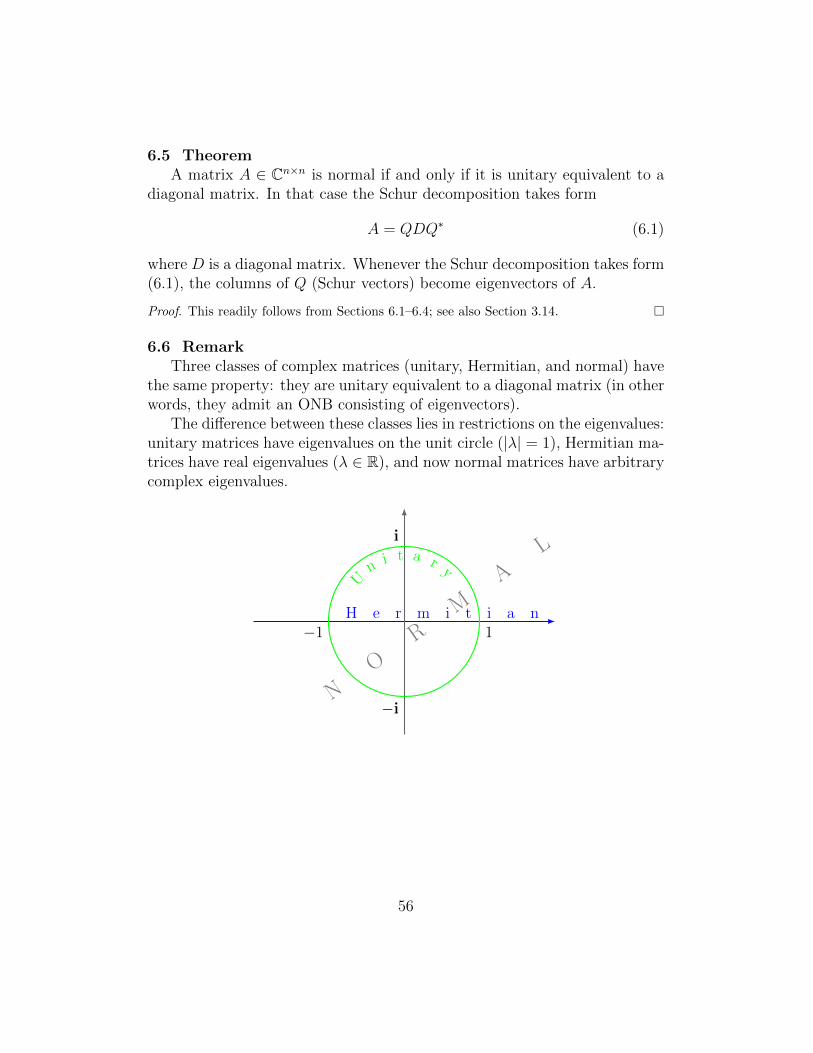
6.5 TheoremA matrix A ∈ Cn×n is normal if and only if it is unitary equivalent to a

diagonal matrix. In that case the Schur decomposition takes form

A = QDQ∗ (6.1)

where D is a diagonal matrix. Whenever the Schur decomposition takes form(6.1), the columns of Q (Schur vectors) become eigenvectors of A.

Proof. This readily follows from Sections 6.1–6.4; see also Section 3.14. �

6.6 RemarkThree classes of complex matrices (unitary, Hermitian, and normal) have

the same property: they are unitary equivalent to a diagonal matrix (in otherwords, they admit an ONB consisting of eigenvectors).

The difference between these classes lies in restrictions on the eigenvalues:unitary matrices have eigenvalues on the unit circle (|λ| = 1), Hermitian ma-trices have real eigenvalues (λ ∈ R), and now normal matrices have arbitrarycomplex eigenvalues.

1−1

i

−i

H e r m i t i a n

Un

i t a r y

N

O

R

M

A

L

56

6.7 Real Schur DecompositionIf A ∈ Rn×n, then there exists an orthogonal matrix Q such that

QTAQ =

R11 R12 · · · R1m

0 R22 · · · R2m...

.... . .

...0 0 · · · Rmm

where each diagonal block Rii is either a 1× 1 matrix or a 2× 2 matrix.

Proof. We use the induction on n. Our induction will be somewhat unusual – its incrementwill be either 1 or 2, i.e., our proof of the theorem for any given n will be based on itsvalidity for either n − 1 or n − 2 (depending on the matrix A). Thus the basis for ourinduction must consist of two smallest values of n, i.e., n = 1 and n = 2.

For n = 1 and n = 2, we just write A = I · A · I∗ and note that I is unitary and A iseither a single 1× 1 block (if n = 1) or a single 2× 2 block (if n = 2).

Now let n > 2. If the matrix A has a real eigenvalue, then we can reduce the dimensionby one just like in the proof in Section 6.1 and then use our inductive assumption of thevalidity of the theorem for n− 1.

If A has no real eigenvalues, then by Lemma 2.16 there is a two-dimensional subspaceW ⊂ Rn invariant under A. Let {x1, x2} be an ONB of W (one exists due to Sect. 1.26).The invariance of W under A implies that Ax1 ∈W and Ax2 ∈W , hence

Ax1 = r11 x1 + r21 x2

Ax2 = r12 x1 + r22 x2

with some rij ∈ R. Due to Sect. 1.26, the ONB {x1, x2} in W can be extended to an

ONB {x1, . . . , xn} in Rn. Let Q denote the orthogonal matrix with columns x1, . . . , xn.Observe that Qe1 = x1 and Qe2 = x2, hence QTx1 = e1 and QTx2 = e2. Therefore,

QTAQe1 = QTAx1 = QT (r11 x1 + r21 x2) = r11 e1 + r21 e2

and similarly

QTAQe2 = QTAx2 = QT (r12 x1 + r22 x2) = r12 e1 + r22 e2

Thus,

QTAQ =

[R11 R12

0 R22

]where

R11 =

[r11 r12

r21 r22

]R12 is some 2 × (n − 2) matrix and R22 is some (n − 2) × (n − 2) matrix. Now we can

apply our inductive assumption to the (n− 2)× (n− 2) matrix R22 and finish the proof in

the same way as the proof in Section 6.1. Note that we need the validity of the theorem

for n− 2, i.e., the increment of our induction is 2 in the above case. �

57

Exercise 6.1. (combined from JPE, October 1990 and May 1997) Let A ∈ Cn×n be anormal matrix.

(a) Prove that A− λI is normal for any λ ∈ C.

(b) Prove that ‖Ax‖ = ‖A∗x‖ for all x.

(c) Prove that (λ, x) is an eigenpair of A if and only if (λ, x) is an eigenpair of A∗.(Hence, A and A∗ have the same eigenvectors.)

Exercise 6.2. (JPE, September 2002) A matrix A ∈ Cn×n is said to be skew Hermitianif A∗ = −A.

(a) Prove that if A is skew Hermitian and B is unitary equivalent to A, then B is alsoskew Hermitian.

(b) Prove that the eigenvalues of a skew Hermitian matrix are purely imaginary, i.e.they satisfy λ = −λ.

(c) What special form does the Schur decomposition take for a skew Hermitian matrixA?

Exercise 6.3. (JPE, September 1998). Show that diagonalizable complex matrices makea dense subset of Cn×n. That is, for any A ∈ Cn×n and ε > 0 there is a diagonalizableB ∈ Cn×n such that ‖A−B‖2 < ε.

Exercise 6.4 (Bonus). (JPE, May 1996). Let T be a linear operator on a finite dimen-sional complex inner product space V , and let T ∗ be the adjoint of T . Prove that T = T ∗

if and only if T ∗T = T 2.

58

Chapter 7

LU Decomposition

First we review Gaussian elimination from Linear Algebra:

7.1 Gaussian eliminationLet A ∈ Cn×n be a square matrix. We will modify it consecutively, in

n − 1 steps, as described below, to obtain an upper triangular matrix. Forthe first step we denote A(1) = A and a

(1)ij = aij for all 1 ≤ i, j ≤ n.

Step 1. Assume that a(1)11 6= 0. We define multipliers

mi1 = a(1)i1 /a

(1)11 for i = 2, . . . , n

Then we replace the i-th row a(1)i of the matrix A(1) with a

(1)i −mi1a

(1)1 for

all i = 2, . . . , n, and obtain a new matrix

A(2) =

a

(1)11 a

(1)12 · · · a

(1)1n

0 a(2)22 · · · a

(2)2n

......

. . ....

0 a(2)n2 · · · a

(2)nn

where

a(2)ij = a

(1)ij −mi1a

(1)1j for 2 ≤ i, j ≤ n

Note that the first column of A(2) below the diagonal consists of zeros, i.e.,a

(2)i1 = 0 for all i = 2, . . . , n.

Step 2. Assume that a(2)22 6= 0. We define multipliers

mi2 = a(2)i2 /a

(2)22 for i = 3, . . . , n

Then we replace the i-th row a(2)i of the matrix A(2) with a

(2)i −mi2a

(2)2 for

59

all i = 3, . . . , n, and obtain a new matrix

A(3) =

a

(1)11 a

(1)12 a

(1)13 · · · a

(1)1n

0 a(2)22 a

(2)23 · · · a

(2)2n

0 0 a(3)33 · · · a

(2)3n

......

.... . .

...

0 0 a(3)n3 · · · a

(3)nn

where

a(3)ij = a

(2)ij −mi1a

(2)2j for 3 ≤ i, j ≤ n

Note that the first two columns of A(3) below the diagonal consists of zeros,i.e., a

(3)ij = 0 for j = 1, 2 and all i = j + 1, . . . , n.

Then we continue this process. At each step we create zeros in one morecolumn below the diagonal. In n − 1 steps all the columns below the maindiagonal will consist of zeros, hence the resulting matrix An will be uppertriangular, and we will denote ir by U :

A(n) = U =

a

(1)11 a

(1)12 a

(1)13 · · · a

(1)1n

0 a(2)22 a

(2)23 · · · a

(2)2n

0 0 a(3)33 · · · a

(3)3n

......

.... . .

...

0 0 0 · · · a(n)nn

Remember that the above procedure requires a

(k)kk 6= 0 for all k = 1, . . . , n−1.

These numbers are called pivots.The procedure has to stop prematurely if (and only if) one of the pivots

happens to be zero. In that case we say that the Gaussian elimination fails.Note that

a(k)kk 6= 0 for all k = 1, . . . , n− 1

is equivalent to

a(1)11 · · · a

(k)kk 6= 0 for all k = 1, . . . , n− 1

This will be convenient for the criterion of failure below.

60

7.2 Principal minorsLet A ∈ Cn×n. For 1 ≤ k ≤ n − 1, the k-th principal minor of A is the

k×k matrix formed by the entries in the first k rows and the first k columnsof A. In other words, Ak is the top left k× k block of A. We denote the k-thprincipal minor of A by Ak. We will also denote An = A.

7.3 Criterion of failureGaussian elimination fails if and only if

detAk = 0 for some k = 1, . . . , n− 1.

This is because for each k = 1, . . . , n

detAk = a(1)11 · · · a

(k)kk .

Next we present the Gaussian elimination in matrix form. All our formu-las can be verified by direct inspection, so we give them without proof.

7.4 Gauss matricesFor each j = 1, . . . , n− 1 we denote

m(j) =

0...0

mj+1,j...

mn,j

and then we define the so called Gauss matrix Gj by

Gj = I −m(j)e∗j =

1 0 · · · 0 · · · 0 00 1 · · · 0 · · · 0 0...

.... . .

.... . .

......

0 0. . . 1 · · · ...

......

.... . . −mj+1,j

. . ....

......

.... . .

...... 1 0

0 0 · · · −mn,j · · · 0 1

.

61

7.5 Main matrix formulasFor each k = 1, . . . , n− 1 we have

A(k+1) = GkA(k)

and thereforeU = A(n) = Gn−1 · · ·G2G1A.

This can be rewritten as

A = G−11 G−1

2 · · ·G−1n−1U.

Next let us denote

Lj = I +m(j)e∗j =

1 0 · · · 0 · · · 0 00 1 · · · 0 · · · 0 0...

.... . .

.... . .

......

0 0 · · · 1 · · · 0 0...

.... . . mj+1,j

. . ....

......

.... . .

.... . . 1 0

0 0 · · · mn,j · · · 0 1

.

For each j = 1, . . . , n− 1 we have LjGj = I, hence G−1j = Lj, and thus

A = L1L2 · · ·Ln−1U. (7.1)

7.6 Unit lower/upper triangular matricesA matrix L is said to be unit lower triangular if it is lower triangular and

has ones on its main diagonal. Note that detL = 1. The following slightextensions of the rules given in Section 0.8 can be verified directly:

• If L1 and L2 are both unit lower triangular matrices, then so is theirproduct L1L2 and so are their inverses L−1

1 and L−12 .

Unit lowertriangularmatrices:

01

1

1

× 01

1

1

= 01

1

1

01

1

1

-1

= 01

1

1

In a similar way we can define unit upper triangular matrices. They obeysimilar rules.

62

7.7 Main matrix formulas (continued)Note that L1, . . . , Ln−1 in (7.1) are unit lower triangular matrices, thus

their product is a unit lower triangular matrix, which we denote by L. Moreprecisely, we have

L = L1L2 · · ·Ln−1

= (I +m(1)e∗1)(I +m(2)e∗2) · · · (I +m(n−1)e∗n−1)

= I +m(1)e∗1 +m(2)e∗2 + · · ·+m(n−1)e∗n−1

=

1 0 0 · · · 0m21 1 0 · · · 0

......

.... . .

...mn−1,1 mn−1,2 · · · 1 0mn1 mn2 · · · mn,n−1 1

.We summarize our matrix formulas in the following theorem:

7.8 Theorem (LU decomposition)Let A ∈ Cn×n have non-singular principal minors up to the order n− 1.

Then there is a decomposition

A = LU

where L is a unit lower triangular matrix and U is an upper triangular matrix:

A

= 01

1

1

L

×0U

Note that detL = 1, hence

detA = detU = u11 · · ·unn.If, in addition, A is non-singular, then the LU decomposition is unique.

Proof : The existence follows from our matrix formulas. To prove the uniqueness, weargue by way of contradiction. Let A = LU = LU be two LU decompositions. Since A isnon-singular, it follows that U is also non-singular, and hence

L−1L = UU−1.

By the rules of Section 7.6, the inverse L−1 is unit lower triangular, so the product L−1Lis unit lower triangular. On the other hand, UU−1 is upper triangular. The only matrixthat is both unit lower triangular and upper triangular is the identity matrix I, hence

L−1L = UU−1 = I.

This implies L = L and U = U . �

63

7.9 Forward and backward substitutionsThe LU decomposition can be used to solve a system of linear equations

Ax = b,

where A ∈ Cn×n is a given nonsingular matrix, b ∈ Cn is a given vector, andand x ∈ Cn is an unknown vector to be computed.

Suppose we have an LU decomposition A = LU , where L is lower trian-gular and U is upper triangular. Then we can find x in two steps.

0

L

×0U

×

x

=

b︸ ︷︷ ︸y

Step 1. Denote Ux = y and solve the lower triangular system Ly = b for yvia “forward substitution” (computing y1, . . . , yn subsequently):

`11y1 = b1 ⇒ y1 = b1/`11

`21y1 + `22y2 = b2 ⇒ y2 = (b2 − `21y1)/`22

`31y1 + `32y2 + `33y3 = b3 ⇒ y3 = (b3 − `31y1 − `32y2)/`33

......

`n1y1 + · · ·+ `nnyn = bn ⇒ yn = (bn − `n1y1 − · · · − `n(n−1)yn−1)/`nn

Note: if L is unit lower triangular, then `11 = · · · = `nn = 1, and thereforethe divisions can be avoided.

Step 2. Solve the system Ux = y for x via “backward substitution” (com-puting xn, . . . , x1 subsequently):

unnxn = yn ⇒ xn = yn/unn

u(n−1)(n−1)xn−1 + u(n−1)nxn = yn−1 ⇒ xn−1 = (yn−1 − u(n−1)nxn)/u(n−1)(n−1)

......

u11x1 + · · ·+ u1nxn = y1 ⇒ x1 = (y1 − u12x2 − · · · − u1nxn)/u11

64

7.10 Cost of computationThe cost of computation is measured in “flops”, where a flop (floating

point operation) is an arithmetic operation (addition, subtraction, multipli-cation, division, or a root extraction).

Let us estimate the cost of the LU decomposition. The cost of computa-tion of A(2) is n− 1 divisions to compute the multipliers and then 2n(n− 1)flops to update the rows (n − 1 rows with 2n flops per row), i.e. total ofapproximately 2n2 flops. The computation of A(3) then takes 2(n−1)2 flops,and so on.

Thus the total computational cost for the LU factorization is

2(n2 + (n− 1)2 + · · ·+ 12

)=

2n(n+ 1)(2n+ 1)

6≈ 2n3

3flops

If one solves a system of linear equations Ax = b, then the LU decompo-sition is followed by solving two triangular systems (Section 7.9). The costto solve one triangular system is about n2 flops. So there is an additionalcost of 2n2 flops, which is negligible compared to 2n3/3. Hence, the totalcost is still ≈ 2n3/3.

Note that the LU decomposition takes most of the computations requiredfor solving a system Ax = b. Thus, this method is particularly well suited tovery common situations in which one is solving systems Ax = b for more thanone vector b, but with the same matrix A. In that case the LU decompositionis done just once, and then each additional b will require ≈ 2n2 flops.

7.11 Computation of A−1

Assume that A ∈ Cn×n is non-singular and has non-singular principalminors up to the order n−1, so that the Gaussian elimination works. One canfind the matrix X = A−1 by solving the system AX = I for X ∈ Cn×n. Thisamounts to solving n systems of linear equations Axk = ek, for k = 1, . . . , n,where xk stands for the k-th column of the matrix X. The computationalcost of this procedure is

2n3

3+ n× 2n2 =

8n3

3flops

As a matter of fact, this is the fastest way of computing the inverse A−1.

65

7.12 “Manual” solution of systems of linear equationsOne needs to remember that the LU decomposition (with the subsequent

forward and backward substitutions) is just a convenient matrix represen-tation of the standard and more familiar Gaussian elimination. These twoprocedures are mathematically equivalent. When one solves a system of lin-ear equations Ax = b practically (on paper), one should definitely apply theGaussian elimination to both A and b, rather than forming the L and Umatrices.

7.13 ExampleSuppose one needs to solve the following system by LU decomposition:[

0.01 21 3

] [xy

]=

[24

]Then one multiplies the first row by 100 and subtracts it from the second row. This gives[

0.01 20 −197

] [xy

]=

[2−196

]Then one solves the second equation for y and finds y = 196

197 . Lastly, one substitutes this

value for y into the first equation and finds x = 200197 .

7.14 WarningsIt is a common practice to solve systems of linear equations Ax = b

with a nonsingular matrix A via Gaussian elimination (or, equivalently, LUdecomposition). However, this method requires that the matrix A satisfiescertain conditions (Section 7.3).

It is easy to find nonsingular matrices for which Gaussian elimination doesnot work and LU decomposition does not exist. For example, let A = [ 0 1

1 0 ].Then the Gaussian elimination fails instantly, because the very first pivot iszero. Furthermore, for this matrix A there is no LU decomposition A = LU ,even if we only require that L be lower triangular (not necessarily unit lowertriangular); see Exercise 7.2.

In addition, when a pivot is not exactly zero but close to zero, then thingscan go wrong, too: multipliers become very large, and numerical computa-tions (in the sense specified later in Chapter 11) tend to become inaccurate.One should avoid such situations by using an appropriate pivoting strategy.We will describe these strategies, briefly, and illustrate them by example.

66

7.15 Partial pivotingThe idea is to avoid zero or small pivots by interchanging rows. At every

step of Gaussian elimination one looks for the largest (in absolute value)element in the pivot column (at or below the main diagonal). Then the rowcontaining the largest element is interchanged with the current row. Nowthe largest element is on the main diagonal. After that the usual eliminationstep is performed.

Partial pivoting ensures that all the multipliers (i.e., the elements of thematrix L) have absolute values less than or equal to one.

7.16 ExampleWe apply the partial pivoting strategy to Example 7.13. In the first column, the larger

element is 1, hence we need to interchange the rows to put that element on the diagonal:[1 3

0.01 2

] [xy

]=

[42

].

Now we multiply the first row by 0.01 and subtract it from the second row. This gives[1 30 1.97

] [xy

]=

[4

1.96

].

Then we solve the second equation for y and find y = 196197 . Lastly, we substitute this value

for y into the first equation and find x = 200197 .

7.17 Complete pivotingThe method of complete pivoting involves both row and column inter-

changes to make use of the largest pivot available. This method providesadditional insurance against buildup of computational errors.

7.18 ExampleWe apply the complete pivoting strategy to Example 7.13. The largest element in the

whole matrix is 3, so we need to move it to the top left position by interchanging rowsand columns: [

3 12 0.01

] [yx

]=

[42

].

Note that interchanging columns requires permutation of the unknowns x and y. Next wemultiply the first row by 2/3 and subtract it from the second row. This gives[

3 10 − 197

300

] [yx

]=

[4− 2

3

].

Then we solve the second equation for x and find x = 200197 . Lastly, we substitute this value

for x into the first equation and find y = 196197 .

67

7.19 Diagonally dominant matricesA matrix A ∈ Cn×n such that

|aii| >∑j 6=i

|aij |

for all i is said to be strictly row diagonally dominant. If

|ajj | >∑i6=j

|aij |

for all j the matrix is said to be strictly column diagonally dominant.

One can check that if a matrix A is strictly row (or column) diagonallydominant, then detA 6= 0 (the proof can be omitted for now; this fact readily follows

from Gershgorin Theorem that will be given in Chapter 15). Since all the principalminors of A are also strictly row (or column) diagonally dominant, we havedetAk 6= 0 for all 1 ≤ k < n. Therefore no zero pivots will be encounteredduring Gaussian elimination.

With some extra effort one can show that if A is strictly column diagonally dominant,

then all the multipliers (i.e., the elements of L) have absolute values ≤ 1.

Exercise 7.1. Find a nonzero matrix A ∈ R2×2 that admits at least two LU decompo-sition, i.e. A = L1U1 = L2U2, where L1 and L2 are two distinct unit lower triangularmatrices and U1 and U2 are two distinct upper triangular matrices.

Exercise 7.2. Show that the matrix

[0 11 0

]admits no LU decomposition, even if we only

require that L be lower triangular (not necessarily unit lower triangular).

Exercise 7.3. The spectral radius of a matrix A ∈ Cn×n is defined by

ρA = max{|λ| : λ eigenvalue of A}.

(a) Show that ρA ≤ ‖A‖2.

(b) Give an example of a 2× 2 matrix A such that ρA < 1 but ‖A‖2 > 100.

(c) Show that iflimn→∞

‖An‖2 = 0,

then ρA < 1.

Exercise 7.4 (Bonus). In the notation of the previous problem, show that if ρA < 1, then

limn→∞

‖An‖2 = 0.

Hint: use Jordan decomposition.

68

Chapter 8

Cholesky Factorization

8.1 Theorem (LDM∗ Decomposition)Assume that A ∈ Cn×n is non-singular and has non-singular principal

minors, i.e., detAk 6= 0 for all k = 1, . . . , n. Then there are unique matricesL,D,M such that L,M are unit lower triangular, D is diagonal, and

A = LDM∗ (8.1)

A

= 01

1

1

L

×0

0

D

×1

1

10M∗

Proof. According to Theorem 7.8, there is an LU decomposition A = LU . Let u11, . . . , unndenote the diagonal components of U . Define diagonal matrix D = diag{u11, . . . , unn}.Since A is non-singular, D is invertible, and D−1 = diag{u−1

11 , . . . , u−1nn}. One can easily

check that M∗ = D−1U is a unit upper triangular matrix, hence (8.1) exists.

To prove the uniqueness, suppose A = LDM∗ = L1D1M∗1 are two different LDM∗

decompositions. Note that all the matrices here are invertible, because A is non-singular.

By the uniqueness of the LU decomposition (Theorem 7.8), we have L = L1, hence,

DM∗ = D1M∗1 and D−1

1 D = M∗1 (M∗)−1. Since both M∗ and M∗1 are unit upper triangu-

lar, so is M∗1 (M∗)−1 (by Sect. 7.6). On the other hand, D−11 D is diagonal. The only matrix

that is unit lower triangular and diagonal is the identity matrix. Thus M∗1 (M∗)−1 = I

and D−11 D = I, which implies M∗ = M∗1 and D = D1. �

8.2 Corollary (LDL∗ Decomposition)Suppose A ∈ Cn×n satisfies the assumptions of Theorem 8.1 and is Hermi-

tian. Then there exist a unique unit lower triangular matrix L and a uniquediagonal matrix D such that

A = LDL∗

Moreover, the components of D are real numbers.

69

Proof. By Theorem 8.1, A = LDM∗. Now A = A∗ = MD∗L∗, and by the uniqueness of

the LDM∗ decomposition we have L = M and D = D∗. The latter implies that D is a

real matrix. �

8.3 Sylvester’s TheoremLet A ∈ Cn×n be a Hermitian matrix. Then

A is positive definite ⇐⇒ detAk > 0 (∀k = 1, . . . , n)

Proof. Let A be positive definite. By Section 4.15, A = B∗B and detB 6= 0. Hence

detA = detB × detB∗ = detB × detB = |detB|2 > 0.

One can easily check that every principal minor Ak is also a Hermitian positive definitematrix, therefore by the same argument detAk > 0.

Now let detAk > 0 for all k = 1, . . . , n. By Corollary 8.2, A = LDL∗. Denote byLk and Dk the k-th principal minors of L and D, respectively. One can easily check thatAk = LkDkL

∗k. Since Lk is unit lower triangular, we have detLk = 1, thus detDk =

detAk > 0. Denote D = diag{d1, . . . , dn}, hence Dk = diag{d1, . . . , dk}. Now

detDk = d1 · · · dk > 0 ∀k = 1, . . . , n

implies that d1, . . . , dn are all real and positive. Lastly,

〈Ax, x〉 = 〈LDL∗x, x〉 = 〈DL∗x, L∗x〉 = 〈Dy, y〉 > 0

where y = L∗x. Note that y 6= 0 whenever x 6= 0, because L∗ is invertible. �

8.4 CorollaryLet A be a positive definite matrix. Then aii > 0 for all i = 1, . . . , n.

Furthermore, let 1 ≤ i1 < i2 < · · · < ik ≤ n, and let A′ be the k × k matrixformed by the intersections of the rows and columns of A with numbersi1, . . . , ik. Then detA′ > 0.

Proof. Recall that A defines an operator Cn → Cn. We can reorder the canonical basis

vectors e1, . . . , en in Cn and get a new ONB {ei1 , . . . , eik , . . .}. In this new basis, the

operator is represented by a matrix B such that Bk = A′, i.e., A′ is a principal minor of

a positive definite matrix. Then we can apply Sylvester’s Theorem 8.3. �

The above corollary suggests a quick way of proving that a given matrix Ais not positive definite: just spot a non-positive diagonal component or a 2×2submatrix (with two components on the diagonal of A) with a non-positivedeterminant, etc.

70

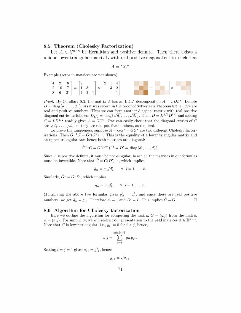
8.5 Theorem (Cholesky Factorization)Let A ∈ Cn×n be Hermitian and positive definite. Then there exists a

unique lower triangular matrix G with real positive diagonal entries such that

A = GG∗

Example (zeros in matrices are not shown):4 2 82 10 78 6 21

=

21 34 2 1

×2 1 4

3 21

= ×

Proof. By Corollary 8.2, the matrix A has an LDL∗ decomposition A = LDL∗. DenoteD = diag{d1, . . . , dn}. As it was shown in the proof of Sylvester’s Theorem 8.3, all di’s arereal and positive numbers. Thus we can form another diagonal matrix with real positivediagonal entries as follows: D1/2 = diag{

√d1, . . . ,

√dn}. Then D = D1/2D1/2 and setting

G = LD1/2 readily gives A = GG∗. One can easily check that the diagonal entries of Gare√d1, . . . ,

√dn, so they are real positive numbers, as required.

To prove the uniqueness, suppose A = GG∗ = GG∗ are two different Cholesky factor-izations. Then G−1G = G∗(G∗)−1. This is the equality of a lower triangular matrix andan upper triangular one; hence both matrices are diagonal:

G−1G = G∗(G∗)−1 = D′ = diag{d′1, . . . , d′n}.

Since A is positive definite, it must be non-singular, hence all the matrices in our formulasmust be invertible. Note that G = G(D′)−1, which implies

gii = gii/d′i ∀ i = 1, . . . , n.

Similarly, G∗ = G∗D′, which implies

gii = giid′i ∀ i = 1, . . . , n.

Multiplying the above two formulas gives g2ii = g2

ii, and since these are real positive

numbers, we get gii = gii. Therefore d′i = 1 and D′ = I. This implies G = G. �

8.6 Algorithm for Cholesky factorizationHere we outline the algorithm for computing the matrix G = (gij) from the matrix

A = (aij). For simplicity, we will restrict our presentation to the real matrices A ∈ Rn×n.Note that G is lower triangular, i.e., gij = 0 for i < j, hence,

aij =

min{i,j}∑k=1

gikgjk.

Setting i = j = 1 gives a11 = g211, hence

g11 =√a11.

71

Next, for 2 ≤ i ≤ n we have ai1 = gi1g11, hence

gi1 = ai1/g11 i = 2, . . . , n.

This gives the first column of G. Now, inductively, assume that we already have the firstj − 1 columns of G. Then ajj =

∑jk=1 g

2jk, hence

gjj =

√√√√ajj −j−1∑k=1

g2jk.

Next, for j + 1 ≤ i ≤ n we have aij =∑jk=1 gikgjk, hence

gij =1

gjj

(aij −

j−1∑k=1

gikgjk

).

8.7 Cost of computationThe computation of gij takes ≈ 2j flops for each i = j, . . . , n, so the total is

n∑j=1

2j(n− j) ≈ 2nn2

2− 2

n3

3=n3

3

Recall that the LU decomposition takes about 2n3/3 flops, so the Cholesky factorization

is nearly twice as fast. It is also more stable than the LU decomposition, in the sense

precisely defined below, in Chapter 13.

8.8 Criterion of positive definitenessThe above algorithm can be used to verify that a given real symmetric

matrix, A, is positive definite. Whenever all the square root extractions inSection 8.6 are possible and give non zero numbers, i.e. whenever

a11 > 0 and ajj −j−1∑k=1

g2jk > 0 ∀j ≥ 2

the matrix A is positive definite. If at least one of the above quantities is notpositive, then A is not positive definite.

Exercise 8.1. (JPE, May 1994) Let A ∈ Rn×n be given, symmetric and positive definite.Define A0 = A, and consider the sequence of matrices defined by

Ak = GkGtk and Ak+1 = GtkGk

where Ak = GkGtk is the Cholesky factorization for Ak. Prove that the Ak all have the

same eigenvalues.

72

Chapter 9

QR Decomposition

9.1 Gram-Schmidt orthogonalization (revisited)Let {v1, . . . , vn} be a linearly independent set of vectors in Cm (m ≥ n).

The Gram-Schmidt orthogonalization described in Section 1.25 gives an or-thonormal set of vectors {u1, . . . , un} in Cm, and the equations (1.14)–(1.16)can be written as

v1 = r11u1,

v2 = r12u1 + r22u2,

v3 = r13u1 + r23u2 + r33u3, (9.1)

. . .

vn = r1nu1 + r2nu2 + · · ·+ rn−1,nun−1 + rnnun

where rip = 〈vp, ui〉 for i < p ≤ n and rpp = ‖wp‖. Note that rpp > 0.Let us assemble a matrix A ∈ Cm×n whose columns are the vectors

v1, . . . , vn, a matrix Q whose columns are the vectors u1, . . . , un:

A =

v1

∣∣∣∣∣∣∣v2

∣∣∣∣∣∣∣· · ·∣∣∣∣∣∣∣vn and Q =

u1

∣∣∣∣∣∣∣u2

∣∣∣∣∣∣∣· · ·∣∣∣∣∣∣∣un .

Let R ∈ Cn×n be an upper triangular matrix defined as follows:

R =

r11 r12 · · · r1n

0 r22 · · · r2n...

.... . .

...0 0 · · · rnn

.Then the above relations (9.1) can be written in matrix form:

A = QR (9.2)

One can verify the equivalence of (9.1) and (9.2) by direct inspection.

73

9.2 Linearly dependent caseLet us relax our assumption that v1, . . . , vn are linearly independent. Thus let {v1, . . . , vn}

be an arbitrary set of vectors in Cm. Then the Gram-Schmidt procedure 1.25 can be ad-justed as follows.

For some p ≥ 1 we now may have vp = 0 or, more generally,

vp ∈ span{v1, . . . , vp−1}.

This implies vp ∈ span{u1, . . . , up−1}, therefore wp = 0, in the notation of Section 1.25.Now the vector up = wp/‖wp‖ cannot be determined.

Instead, we can choose up as an arbitrary unit vector orthogonal to u1, . . . , up−1 (weknow that such vectors exist due to Sect. 1.26). After such a “loosely constrained” selectionof up we continue the Gram-Schmidt orthogonalization as described in Section 1.25. Everytime we encounter a linear dependence vp ∈ span{v1, . . . , vp−1}, we select up “frivolously”as specified above. In that case, the respective equation

vp = r1pu1 + · · ·+ rp−1,pup−1 + rppup

for vp, as given in (9.1), will still hold, but with rpp = 0 instead of rpp > 0.

9.3 Extension of Q to QThe vectors u1, . . . , un make an orthonormal set in Cm that can be ex-

tended to an ONB {u1, . . . , um}, according to Sect. 1.26. Now we can forma larger, square matrix

Q =

u1

∣∣∣∣∣∣∣∣∣∣∣∣u2

∣∣∣∣∣∣∣∣∣∣∣∣· · ·

∣∣∣∣∣∣∣∣∣∣∣∣un

∣∣∣∣∣∣∣∣∣∣∣∣· · ·

∣∣∣∣∣∣∣∣∣∣∣∣um

∈ Cm×m

which is unitary, according to Sect. 2.4. By adding m − n rows consistingof zeros to the bottom of the matrix R we get a larger matrix

R =

r11 r12 · · · r1n

0 r22 · · · r2n

......

. . ....

0 0 · · · rnn0 0 · · · 0...

.... . .

...0 0 · · · 0

∈ Cm×n.

We still call R an “upper triangular matrix”. Now the relation (9.2) can bewritten as

A = QR. (9.3)

The equivalence of (9.2) and (9.3) can be verified by direct inspection.

74

We summarize the previous constructions as follows:

9.4 Theorem (QR decomposition)For any matrix A ∈ Cm×n with m ≥ n there exist a unitary matrix

Q ∈ Cm×m and an upper triangular matrix R ∈ Cm×n such that

A = QR. (9.4)

This is called (full) QR decomposition of A.The first (left) n columns of the matrixQ form a smaller matrix Q ∈ Cm×n

(whose columns are orthonormal vectors in Cm) and the first (upper) n rowsof the matrix R form a square upper triangular matrix R so that

A = QR. (9.5)

This is called reduced (“skinny”) QR decomposition of A.

=

A

×

Q

=

0

R

×

Q

0

R

Proof. Given a matrix A ∈ Cm×n, we disassemble it into column vectors v1, . . . , vn ∈ Cm,

and then apply all the constructions described in Sections 9.1–9.3. �

9.5 Real QR decompositionSuppose A ∈ Rm×n is a real matrix. Then all the constructions of Sec-

tions 9.1–9.3 can be done with real matrices only, and they produce realmatrices Q and R. In particular, Q will be an orthogonal matrix.

9.6 Positivity of the diagonal of RThe QR decomposition can be constructed so that the diagonal compo-

nents of R (R) are real non-negative numbers:

rii ≥ 0 ∀i = 1, . . . , n.

If A has full rank (i.e., rankA = n), then the columns of A are linearlyindependent. In that case R is invertible, and one can construct R (and R)so that its diagonal components are real positive numbers:

rii > 0 ∀i = 1, . . . , n.

75

9.7 Uniqueness of the QR decompositionIf A has full rank (i.e., rankA = n), then the matrix R with real positive

diagonal entries (rii > 0) is unique. The corresponding matrix Q is unique,too.

Proof. Let A = QR = Q1R1 be two different reduced QR decompositions with the specifiedproperties. Then

A∗A = R∗R

because Q∗Q = I is the identity matrix (this follows from the columns of Q being or-thonormal vectors). Similarly,

A∗A = R∗1R1.

Thus we get two Cholesky factorizations for the same matrix A∗A. But this matrix is

positive definite (due to Section 4.18), hence its Cholesky factorization must be unique

(cf. Section 8.5). This implies R = R1. Lastly, Q1 = QRR−11 = Q. �

9.8 Cost of QRIn order to compute the reduced QR decomposition (9.5), one needs to apply Gram-

Schmidt orthogonalization to the n columns of the matrix A and compute the n columnsu1, . . . , un of the matrix Q. The vector up is found by

wp = vp −p−1∑i=1

〈vp, ui〉ui, and up =wp‖wp‖

,

see Section 1.25. Here each scalar product 〈vp, ui〉 requires m multiplications and madditions, and then subtracting every term 〈vp, ui〉ui from vp requiresmmultiplication andm subtractions, for each i = 1, . . . , p. The total is 4mp flops. The subsequent computationof ‖wp+1‖ and then up+1 requires 3m flops, which is a relatively small number, and weignore it. The total flop count is

∑np=1 4mp ≈ 2mn2 flops, i.e., the QR takes

2mn2 flops

9.9 Cost of SVDThere is no finite algorithms for the computation of SVD described in Chapter 5 (ex-

cept for small matrices, see Remark 5.6). The reason will be discussed later in Chapter 15.In practice, the SVD is computed by special iterative algorithms. The computation of thereduced SVD requires approximately

2mn2 + 11n3 flops

76

9.10 Modified Gram-Schmidt orthogonalizationThe algorithm from Section 1.25 is often called classical Gram-Schmidt

orthogonalization, as opposed to the modified Gram-Schmidt orthogonaliza-tion we present next. Given a linearly independent set of vectors {v1, . . . , vn}in Cm, we denote v

(1)i = vi for i = 1, . . . , n, then compute

u1 = v(1)1 /‖v(1)

1 ‖,

and then modify all the remaining vectors by the rule

v(2)i = v

(1)i − 〈v

(1)i , u1〉u1 for 1 < i ≤ n.

After that, inductively, for each p ≥ 2 we compute

up = v(p)p /‖v(p)

p ‖,

and then modify all the remaining vectors by the rule

v(p+1)i = v

(p)i − 〈v

(p)i , up〉up for p < i ≤ n.

The modified and classical Gram-Schmidt methods produce the same or-thonormal basis {u1, . . . , un} (i.e., these two methods are mathematicallyequivalent). They are based on a different logic, though.

The classical Gram-Schmidt computes up by making the current vectorvp orthogonal to all the previously constructed vectors u1, . . . , up−1, withouttouching the remaining vectors vp+1, . . . , vn. The amount of work increasesas p grows from 1 to n. This is a “lazy man schedule” - do as little as possibleand leave the rest of the work “for later”.

The modified Gram-Schmidt computes up and makes all the remainingvectors vp+1, . . . , vn orthogonal to it. Once this is done, the remaining vectorswill be in the orthogonal complement to the subspace span{u1, . . . , up} andthere is no need to involve the previously constructed vectors anymore. Theamount of work decreases as p grows from 1 to n. This is an “industriousman schedule” - do as much as possible now and reduce the workload.

Overall, both methods require the same amount of flops. But the mod-ified Gram-Scmidt has an important advantage that it gives more accuratenumerical results in computer calculations; see programming assignment.

77

Classical Gram-Schmidt:

w1=v1 u1 = w1

‖w1‖

w2=v2−〈v2, u1〉u1 u2 = w2

‖w2‖

w3=v3−〈v3, u1〉u1−〈v3, u2〉u2 u3 = w3

‖w3‖

w4=v4−〈v4, u1〉u1−〈v4, u2〉u2−〈v4, u3〉u3 u4 = w4

‖w4‖

......

...

wp=vp−〈vp, u1〉u1−〈vp, u2〉u2 − · · · −〈vp, up−1〉up−1 up = wp‖w4‖

......

......

The amount of work increases at each step (the red rows grow longer)

Modified Gram-Schmidt:

w1=v1 u1 = w1

‖w1‖

w2=v2−〈v2, u1〉u1 u2 = w2

‖w2‖

w3=v3−〈v3, u1〉u1−〈v3, u2〉u2 u3 = w3

‖w3‖

w4=v4−〈v4, u1〉u1−〈v4, u2〉u2−〈v4, u3〉u3 u4 = w4

‖w4‖

......

...

wp=vp−〈vp, u1〉u1−〈vp, u2〉u2 − · · · −〈vp, up−1〉up−1 up = wp‖w4‖

......

......

The amount of work decreases at each step (the red columns get shorter)

78

Exercise 9.1. (JPE, September 2002) Consider three vectors

v1 =

1ε00

, v2 =

10ε0

, v3 =

100ε

.

where ε� 1.

(a) Use the classical Gram-Schmidt method to compute 3 orthonormal vectors q1, q2, q3,making the approximation that 1 + ε2 ≈ 1 (that is, replace any term containing ε2

or smaller with zero, but retain terms containing ε). Are qi (i = 1, 2, 3) pairwiseorthogonal? If not, why not?

(b) Repeat (a) using the modified Gram-Schmidt orthogonalization process. Are theqi(i = 1, 2, 3) pairwise orthogonal? If not, why not?

79

Chapter 10

Least Squares

10.1 DefinitionA system of linear equations Ax = b with A ∈ Cm×n, x ∈ Cn and b ∈ Cm,

is said to be overdetermined if m > n. Since there are more equations thanunknowns, the system usually has no solutions; so we will write it as Ax ≈ b.

10.2 Conditions for existence and uniqueness of a solutionRecall that every matrix A ∈ Cm×n defines a linear transformation Cn → Cm.

Since it takes a smaller space into a larger one, its range is a proper subset of Cm.

CnRangeA Cm

A

It is clear that the equation Ax = b has a solution if and only if b ∈ RangeA.

In the latter case the solution is unique if and only if our linear transformation is

injective. The latter occurs if and only if KerA = {0} (cf. Section 0.6).

10.3 Least squares solutionLet Ax ≈ b be an overdetermined linear system. A vector x ∈ Cn that

minimizes the functionE(x) = ‖b− Ax‖2

is called a least squares solution of Ax ≈ b. The vector r = b− Ax is calledthe residual vector and ‖r‖2 the residual norm.

10.4 Normal equationsLet Ax ≈ b be an overdetermined linear system. The linear system

A∗Ax = A∗b (10.1)

is called the system of normal equations associated with Ax ≈ b.

Note that A∗A ∈ Cn×n, hence (10.1) is an ordinary system of linear equations

(not an overdetermined system).

80

10.5 TheoremLet Ax ≈ b be an overdetermined linear system. Then

(a) A vector x minimizes E(x) = ‖b − Ax‖2 if and only if it is an exactsolution of the system Ax = b, where b is the orthogonal projection ofb onto RangeA.

(b) A vector x minimizing E(x) always exists. It is unique if and only if Ahas full rank (equivalently, KerA = {0}).

(c) A vector x minimizes E(x) if and only if it is a solution of the systemof normal equations A∗Ax = A∗b.

Proof. Denote W = RangeA. We have an orthogonal decomposition Cm = W ⊕W⊥,in particular b = b + r, where b ∈ W and r ∈ W⊥ are uniquely determined by b. NowPythagorean Theorem 1.16 gives

[E(x)]2 = ‖b−Ax‖22 = ‖ b− b︸ ︷︷ ︸=r∈W⊥

+ b−Ax︸ ︷︷ ︸∈W

‖2

= ‖r‖22 + ‖b−Ax‖22 ≥ ‖r‖22

Hence, minxE(x) = ‖r‖2 is attained whenever Ax = b. Since b ∈ RangeA, there is always

a vector x ∈ Cn such that Ax = b. The vector x is unique whenever the map A : Cn → Cmis injective, i.e., whenever KerA = {0}, i.e., whenever A has full rank. This proves (a)and (b).

To prove (c), recall that (RangeA)⊥ = KerA∗ (by Section 3.7), therefore r = b− b ∈KerA∗. Moreover, b − Ax ∈ KerA∗ if and only if Ax = b, because b and r are uniquelydetermined by b. Now

x minimizes E(x) ⇔ Ax = b ⇔ Ax− b ∈ KerA∗ ⇔ A∗Ax = A∗b

The proof is complete. �

Cn

b

b

r

W = RangeA

W⊥

Cm

A

81

Next we give examples that lead to overdetermined systems and leastsquares problems.

10.6 Linear least squares fitLet (xi, yi), 1 ≤ i ≤ m, be points in the xy plane. For any straight line

y = a0 +a1x one defines the “combined distance” from that line to the givenpoints by

E(a0, a1) =

[ m∑i=1

(a0 + a1xi − yi)2

]1/2

The line y = a0 +a1x that minimizes the function E(a0, a1) is called the leastsquares fit to the points (xi, yi). This is a basic tool in statistics. Let

A =

1 x1

1 x2...

...1 xm

x =

[a0

a1

]b =

y1

y2...ym

Then

E(a0, a1) = ‖b− Ax‖2

Hence the least squares fit is equivalent to the least squares problem Ax ≈ b.

10.7 Polynomial least squares fitGeneralizing 10.6, one can fit a polynomial y = p(x) = a0+a1x+· · ·+anxn

of degree n ≥ 2 to a set of data points (xi, yi), 1 ≤ i ≤ m, with m > n + 1.The least squares fit is based on minimizing the function

E(a0, . . . , an) =

[ m∑i=1

(a0 + a1xi + · · ·+ anx

ni − yi

)2]1/2

This is equivalent to the least squares problem for an overdetermined linearsystem

a0 + a1xi + · · ·+ anxni ≈ yi 1 ≤ i ≤ m

in which a0, . . . , an are unknowns.

82

10.8 Continuous least squares fitInstead of fitting a polynomial p(x) ∈ Pn(R) of degree n to a discrete data set (xi, yi)

one can fit it to a continuous function y = f(x) on [0, 1]. The least squares fit is based onminimization of

E(a0, . . . , an) =

[∫ 1

0

|f(x)− p(x)|2 dx]1/2

The solution to this problem is the orthogonal projection of f(x) onto Pn(R).To find the solution, we use the basis {1, x, . . . , xn} in Pn(R). Then a0, . . . , an can be

found by solving the system of equations (analogous to normal equations)

n∑j=0

aj〈xj , xi〉 = 〈f, xi〉 1 ≤ i ≤ n.

The matrix of coefficients here is

〈xj , xi〉 =

∫ 1

0

xi+j dx =1

1 + i+ j

for 0 ≤ i, j ≤ n.

Next we present three computer algorithms for solving the least square prob-lem.

10.9 Algorithm 1, based on normal equationsThis is the simplest one:

1. Form the matrix A∗A and the vector A∗b.2. Compute the Cholesky factorization A∗A = GG∗.3. Solve the lower-triangular system Gz = A∗b for z by forward substitution 7.9.4. Solve the upper-triangular system G∗x = z for x by backward substitution 7.9.

The cost of this algorithm is dominated by Steps 1 and 2. Because the matrix A∗A issymmetric, its computation requires mn(n + 1) ≈ mn2 flops. The computation of A∗brequires only 2mn flops, a relatively small amount which we can ignore. The Choleskyfactorization takes n3/3 flops (cf. Section 8.7). Hence the total cost is

≈ mn2 + 13n

3 flops

Note: the above method is a computer algorithm. For manual work (onpaper), solving the least squares problem by using normal equations meansthe following: you compute the matrix A∗A and the vector A∗b and then solvethe system A∗Ax = A∗b for x any way you want (by Gaussian elimination,for example).

83

10.10 Algorithm 2, based on QR decompositionUsing the reduced QR decomposition (Section 9.5) allows us to rewrite the system of

normal equations asR∗Q∗QRx = R∗Q∗b

If A has full rank, the matrix R∗ is nonsingular and we cancel it out. Also, since thecolumns of Q are orthonormal vectors, Q∗Q = I. Hence

Rx = Q∗b

This suggests the following algorithm:

1. Compute the reduced QR decomposition A = QR.2. Compute the vector Q∗b.3. Solve the upper-triangular system Rx = Q∗b for x by backward substitution 7.9.

The cost of this algorithm is dominated by Step 1, the reduced QR factorization, whichrequires

≈ 2mn2 flops

see Section 9.8. This is approximately twice as much as Algorithm 1 takes.

10.11 Algorithm 3, based on SVDUsing the reduced SVD (Section 5.7) allows us to rewrite the system of normal equa-

tions asV DU∗UDV ∗x = V DU∗b

The matrix V is unitary, and we cancel it out. If A has full rank, the matrix D isnonsingular and we cancel it, too. Since the columns of U are orthonormal vectors,U∗U = I. Hence

DV ∗x = U∗b

This suggests the following algorithm:

1. Compute the reduced SVD decomposition A = UDV ∗.2. Compute the vector U∗b.3. Solve the diagonal system Dz = U∗b for z.4. Compute x = V z.

The cost of this algorithm is dominated by step 1, the reduced SVD decomposition, whichrequires

≈ 2mn2 + 11n3 flops

see Section 9.9. This is approximately the same amount as in Algorithm 2 for m� n, but

for n ≈ m this algorithm is much more expensive.

84

Algorithm 1 is the simplest and the cheapest, but it often gives inaccurateresults in numerical calculations. Algorithms 2 and 3 are more complicatedand expensive (in terms of flops), but usually give more accurate numericalresults, for the reasons we learn in the next chapters.

10.12 Rank deficient matrix AIf rankA < n, then the least squares solution is not unique: the set of

solutions is {x ∈ Cn : Ax = b}, which is a line or a plane in Cn parallel toKerA. In this case the “best” solution is the one of minimal norm:

Axbest = b and ‖xbest‖2 ≤ ‖x‖2 ∀x : Ax = b

Algorithms 1 and 2 fail to find any solution for a rank deficient matrix A. Onthe contrary, Algorithm 3 easily finds the minimal norm solution as follows.

When solving the diagonal system Dz = U∗b for z, we just set zi = 0whenever dii = 0 (in that case (U∗b)i = 0 automatically). This obviouslygives a minimal norm vector z. Since ‖x‖2 = ‖V z‖2 = ‖z‖2, we get aminimal norm vector x as well.

Exercise 10.1. (JPE, September 1997) Let

A =

3 30 44 −1

, and b =

2−2

1

Use the Gram-Schmidt process to find an orthonormal basis for the column space of A.Factor A into a product QR where Q ∈ R3×2 has an orthonormal set of column vectorsand R ∈ R2×2 is upper triangular. Solve the least squares problem Ax = b. Compute thenorm of the residual vector, ‖r‖.

Exercise 10.2. (JPE, May 1998) Given the data (0,1), (3,4) and (6,5), use a QR factor-ization technique to find the best least squares fit by a linear function. Also, solve theproblem via the system of normal equations.

85

Chapter 11

Machine Arithmetic

11.1 Decimal number systemIn our decimal system, natural numbers are represented by a sequence of

digits. For example, 582 = 5 · 102 + 8 · 10 + 2. Generally,

an · · · a1a0 = 10nan + · · ·+ 10a1 + a0,

where ai ∈ {0, 1, 2, 3, 4, 5, 6, 7, 8, 9} are digits. Fractional numbers require anadditional fractional part:

f = .d1d2 . . . dt . . . = 10−1d1 + 10−2d2 + · · ·+ 10−tdt + · · ·

which may be finite or infinite.

11.2 Floating point representationAlternatively, any real number can be written as a product of a fractional

part with a sign and a power of ten:(±.d1d2 . . . dt . . .

)× 10e

where di are decimal digits and e ∈ Z is an integer. For example,

58.2 = 0.582× 102 = 0.0582× 103, etc. (11.1)

This is called floating point representation of decimal numbers. The part.d1d2 . . . dt . . . is called mantissa and e is called exponent. By changing theexponent e with a fixed mantissa .d1d2 . . . dt . . . we can move (“float”) thedecimal point, for example 0.582× 102 = 58.2 and 0.582× 101 = 5.82.

86

11.3 Normalized floating point representationTo avoid unnecessary multiple representations of the same number, such

as in (11.1), we can require that d1 6= 0. We say the floating point repre-sentation is normalized if d1 6= 0. Then 0.582 × 102 is the only normalizedrepresentation of the number 58.2.

For every positive real r > 0 there is a unique integer e ∈ Z such thatf = 10−er ∈ [0.1, 1). Then r = f × 10e is the normalized representation of r.For most of real numbers, the normalized representation is unique, however,there are exceptions, such as(

.9999 . . .)× 100 =

(.1000 . . .

)× 101,

both representing the number r = 1. In such cases one of the two representa-tions has a finite fractional part and the other has an infinite fractional partwith trailing nines.

11.4 Binary number systemIn the binary number system, the base is 2 (instead of 10), and there

are only two digits: 0 and 1. Any natural number N can be written, in thebinary system, as a sequence of binary digits:

N = (an · · · a1a0)2 = 2nan + · · ·+ 2a1 + a0

where ai ∈ {0, 1}. For example, 5 = 1012, 11 = 10112, 64 = 10000002, etc.Binary system, due to its simplicity, is used by all computers. In the moderncomputer world, the word bit means binary digit.

Fractional numbers require an additional fractional part:

f = (.d1d2 . . . dt . . .)2 = 2−1d1 + 2−2d2 + · · ·+ 2−tdt + · · ·

which may be finite or infinite. For example, 0.5 = 0.12, 0.625 = 0.1012, and

0.6 = (0.10011001100110011 . . .)2

(the blocks 00 and 11 alternate indefinitely). The floating point representa-tion of real numbers in the binary system is given by

r =(±.d1d2 . . . dt . . .

)2× 2e

where .d1d2 . . . dt . . . is called mantissa and e ∈ Z is called exponent. Again,we say that the above representation is normalized if d1 6= 0, this ensuresuniqueness for almost all real numbers. Note that d1 6= 0 implies d1 = 1, i.e.,every normalized binary representation begins with a one.

87

11.5 Other number systemsWe can use a number system with any fixed base β ≥ 2. By analogy

with Sections 11.1 and 11.4, any natural number N can be written, in thatsystem, as a sequence of digits:

N = (an · · · a1a0)β = βnan + · · ·+ βa1 + a0

where ai ∈ {0, 1, . . . , β − 1} are digits. Fractional numbers require an addi-tional fractional part:

f = .d1d2 . . . dt . . . = β−1d1 + β−2d2 + · · ·+ β−tdt + · · ·

which may be finite or infinite. The floating point representation of realnumbers in the system with base β is given by

r =(±.d1d2 . . . dt . . .

)β× βe

where .d1d2 . . . dt . . . is called mantissa and e ∈ Z is called exponent. Again,we say that the above representation is normalized if d1 6= 0, this ensuresuniqueness for almost all real numbers.

In the real world, computers can only handle a certain fixed number of digits in their

electronic memory. For the same reason, possible values of the exponent e are always

limited to a certain fixed interval. This motivates our next definition.

11.6 Machine number systems (an abstract version)A machine number system is specified by four integers, (β, t, L, U), where

β ≥ 2 is the baset ≥ 1 is the length of the mantissaL ∈ Z is the minimal value for the exponent eU ∈ Z is the maximal value for the exponent e (of course, L ≤ U).

Real numbers in a machine system are represented by

r =(±.d1d2 . . . dt

)β× βe, L ≤ e ≤ U (11.2)

The representation must be normalized, i.e., d1 6= 0.

88

11.7 Basic properties of machine systemsSuppose we use a machine system with parameters (β, t, L, U). There are finitely many

real numbers that can be represented by (11.2). More precisely, there are

2(β − 1)βt−1(U − L+ 1)

such numbers. The largest machine number is

M =(.(β − 1)β . . . β

)β× βU = βU (1− β−t).

The smallest positive machine number is

m =(.10 . . . 0

)β× βL = βL−1.

Note that zero cannot be represented in the above format, since we require d1 6= 0. For

this reason, every real machine systems includes a few special numbers, like zero, that

have to be represented differently. Other “special numbers” are +∞ and −∞.

11.8 Two standard machine systemsMost modern computers conform to the IEEE floating-point standard (ANSI/IEEE

Standard 754-1985), which specifies two machine systems:

I© Single precision is defined by β = 2, t = 24, L = −125 and U = 128.

II© Double precision is defined by β = 2, t = 53, L = −1021 and U = 1024.

11.9 Rounding rulesA machine system with parameters (β, t, L, U) provides exact represen-

tation for finitely many real numbers. Other real numbers have to be ap-proximated by machine numbers. Suppose x 6= 0 be a real number withnormalized floating point representation

x =(±0.d1d2 . . .

)β× βe

where the number of digits may be finite or infinite.If e > U or e < L, then x cannot be properly represented in the machine system (it

is either “too large” or “too small”). If e < L, then x is usually converted to the special

number zero. If e > U , then x is usually converted to the special number +∞ or −∞.

If e ∈ [L,U ] is within the proper range, then the mantissa of x has tobe reduced to t digits (if it is longer than that or infinite). There are twostandard versions of such reductions:

(a) keep the first t digits and chop off the rest;

(b) round off to the nearest available, i.e. use the rules{.d1 . . . dt if dt+1 < β/2.d1 . . . dt + .0 . . . 01 if dt+1 ≥ β/2

89

11.10 Relative errorsLet x be a real number and xc its computer representation in a machine

system with parameters (β, t, L, U), as described above. We will always assume

that x is neither too big nor too small, i.e., its exponent e is within the proper range

L ≤ e ≤ U . How accurately does xc represent x? (How close is xc to x?)The absolute error of the computer representation, i.e., xc − x, may be

quite large when the exponent e is big. It is more customary to describe theaccuracy in terms of the relative error (xc − x)/x as follows:

xc − xx

= ε or xc = x(1 + ε).

It is easy to see that the maximal possible value of |ε| is

|ε| ≤ u =

{β1−t for chopped arithmetic (a)

12β1−t for rounded arithmetic (b)

The number u is called unit roundoff or machine epsilon.

11.11 Machine epsilonNote that the machine epsilon u is not the smallest positive number m

represented by the given machine system (cf. Sect. 11.7).One can describe u as the smallest positive number ε > 0 such that

(1 + ε)c 6= 1. In other words, u is the smallest positive value that, whenadded to one, yields a result different from one.

In more practical terms, u tells us how many accurate digits machinenumbers can carry. If u ∼ 10−p, then any machine number xc carries atmost p accurate decimal digits.

For example, suppose for a given machine system u ∼ 10−7 and a machine number

xc representing some real number x has value 35.41879236 (when printed on paper or

displayed on computer screen). Then we can say that x ≈ 35.41879, and the digits of x

beyond 9 cannot be determined. In particular, the digits 236 in the printed value of xc

are meaningless (they are “trash” to be discarded).

11.12 Machine epsilon for the two standard machine systemsI© For the IEEE floating-point single precision standard with chopped

arithmetic u = 2−23 ≈ 1.2× 10−7. In other words, approximately 7 decimaldigits are accurate.

II© For the IEEE floating-point double precision standard with choppedarithmetic u = 2−52 ≈ 2.2×10−16. In other words, approximately 16 decimaldigits are accurate.

90

In the next two examples, we will solve systems of linear equations byusing the rules of a machine system. In other words, we will pretend that weare computers. This will help us understand how real computers work.

11.13 ExampleLet us solve the system of equations[

0.01 21 3

] [xy

]=

[24

]The exact solution was found in Section 7.13:

x = 200197 ≈ 1.015 and y = 196

197 ≈ 0.995.

Now let us solve this system by using chopped arithmetic with base β = 10 and t = 2 (i.e.,our mantissa will be always limited to two decimal digits).

First we use Gaussian elimination (without pivoting). Multiplying the first equationby 100 and subtracting it from the second gives −197y = −196. Both numbers 197 and196 are three digit long, so we must chop the third digit off. This gives −190y = −190,hence y = 1. Substituting y = 1 into the first equation gives 0.01x = 2 − 2 = 0, hencex = 0. Thus our computed solution is

xc = 0 and yc = 1.

The relative error in x is (xc − x)/x = −1, i.e., the computed xc is 100% off mark!Let us increase the length of mantissa to t = 3 and repeat the calculations. This gives

xc = 2 and yc = 0.994.

The relative error in x is now (xc − x)/x = 0.97, i.e., the computed xc is 97% off mark.Not much of improvement... We postpone the explanation until Chapter 13.

Let us now apply partial pivoting (Section 7.15). First we interchange the rows:[1 3

0.01 2

] [xy

]=

[42

].

Now we multiply the first equation by 0.01 and subtract it from the second to get 1.97y =1.96. With t = 2, we must chop off the third digit in both numbers: 1.9y = 1.9, hencey = 1. Substituting y = 1 into the fits equation gives x+ 3 = 4, hence x = 1, i.e.,

xc = 1 and yc = 1.

This is a great improvement over the first two solutions (without pivoting). The relativeerror in x is now (xc − x)/x = −0.015, so the computed xc is only 1.5% off. The relativeerror in y is even smaller (about 0.005).

91

Machine arithmetic Exact arithmetic: Machine arithmeticwith t = 2: with t = 3:

0.01x+ 2y = 2

x+ 3y = 4⇓

0.01x+ 2y = 2

−190y =− 190

Chopping off

←−−−−−−0.01x+ 2y = 2

−197y = −196⇓ ⇓

0.01x+ 2y = 2

y = 1

0.01x+ 2y = 2

y = 196197 ≈ 0.9949

Chopping off

−−−−−−→0.01x+ 2y = 2

y = 0.994⇓ ⇓ ⇓

0.01x = 2− 2 = 0

y = 1

!!© 0.01x = 2− 392197 = 2

197

y = 196197

!!© 0.01x = 2− 1.98�A8 = 0.02

y = 0.994⇓ ⇓ ⇓

x = 0

y = 1

x = 200197 ≈ 1.0152

y = 196197 ≈ 0.9949

x = 2

y = 0.994

Example 11.13 without pivoting.

Machine arithmetic Exact arithmetic: Machine arithmeticwith t = 2: with t = 3:

x+ 3y = 4

0.01x+ 2y = 2⇓

x+ 3y = 4

1.9y = 1.9

Chopping off

←−−−−−−−x+ 3y = 4

1.97y = 1.96⇓ ⇓

x+ 3y = 4

y = 1

x+ 3y = 4

y = 196197 ≈ 0.9949

Chopping off

−−−−−−−→x+ 3y = 4

y = 0.994⇓ ⇓ ⇓

x = 4− 3 = 1

y = 1

x = 4− 588197 = 200

197

y = 196197

x = 4− 2.98�A2 = 1.02

y = 0.994

Example 11.13 with partial pivoting.

92

Now let us continue the partial pivoting with t = 3. We can keep three digits, so1.97y = 1.96 gives y = 1.96/1.97 ≈ 0.9949, which we have to reduce to y = 0.994.Substituting this value of y into the first equation gives x + 2.982 = 4, which we have toreduce to x+ 2.98 = 4, hence x = 1.02. So now

xc = 1.02 and yc = 0.994.

The relative error in x is (xc − x)/x = 0.0047, less than 0.5%.The table below shows the relative error of the numerical solution xc by Gaussian

elimination with pivoting and different lengths of mantissa. We see that the relative erroris roughly proportional to the “typical” round-off error 10−t, with a factor of about 2 to5. We can hardly expect a better accuracy.

relative error typical error factort = 2 1.5× 10−2 10−2 1.5t = 3 4.7× 10−3 10−3 4.7t = 4 2.2× 10−4 10−4 2.2

Conclusions: Gaussian elimination without pivoting may lead to catastrophic errors, which

will remain unexplained until Chapter 13. Pivoting is more reliable – it seems to provide

nearly maximum possible accuracy here. But see the next example...

11.14 ExampleLet us solve another system of equations:[

3 11 0.35

] [xy

]=

[5

1.7

]The exact solution here is

x = 1 and y = 2.

The largest coefficient, 3, is at the top left corner already, so pivoting (partial or complete)would not change anything.

Solving this system in chopped arithmetic with β = 10 and t = 2 gives xc = 0 andyc = 5, which is 150% off. Increasing the length of the mantissa to t = 3 gives xc = 0.883and yc = 2.35, so the relative error is 17%. With t = 4, we obtain xc = 0.987 andyc = 2.039, now the relative error is 2%. The table below shows that the relative errorof the numerical solutions is roughly proportional to the typical round-off error 10−t, butwith a big factor fluctuating around 150 or 200.

relative error typical error factort = 2 1.5× 10−0 10−2 150t = 3 1.7× 10−1 10−3 170t = 4 2.0× 10−2 10−4 200

We postpone a complete analysis of the above two examples until Chapter 13.

93

11.15 Computational errorsLet x and y be two real numbers represented in a machine system by xc

and yc, respectively. An arithmetic operation x ∗ y (where ∗ stands for oneof the four basic operations: +,−,×,÷) is performed by a computer in thefollowing way. The computer first finds xc ∗ yc exactly and then representsthat number in its machine system. The result is z = (xc ∗ yc)c.

Note that, generally, z is different from (x ∗ y)c, which is the machine representation

of the exact result x ∗ y. Hence, z is not necessarily the best representation for x ∗ y. In

other words, the computer makes additional round off errors at each arithmetic operation.

Assuming that xc = x(1 + ε1) and yc = y(1 + ε2) we have

(xc ∗ yc)c = (xc ∗ yc) (1 + ε3) = [x(1 + ε1) ] ∗ [ y(1 + ε2) ] (1 + ε3)

where |ε1|, |ε2|, |ε3| ≤ u.

11.16 Multiplication and divisionFor multiplication, we have

z = xy(1 + ε1)(1 + ε2)(1 + ε3) ≈ xy(1 + ε1 + ε2 + ε3)

(here we ignore higher order terms like ε1ε2), so the relative error is (approx-imately) bounded by 3u. A similar estimate can be made for division:

z =x(1 + ε1)(1 + ε3)

y(1 + ε2)≈ x

y(1 + ε1 − ε2 + ε3).

Note: we used Taylor expansion

1

1 + ε2= 1− ε2 + ε2

2 − ε32 + · · ·

and again ignored higher order terms.

Thus again the relative error is (approximately) bounded by 3u.

Conclusion: machine multiplication and machine division magnify rela-tive errors by a factor of three, at most.

94

11.17 Addition and subtractionFor addition, we have

z = (x+ y + xε1 + yε2)(1 + ε3) = (x+ y)(

1 +xε1 + yε2

x+ y

)(1 + ε3).

Again ignoring higher order terms we can bound the relative error of z by

|x|+ |y||x+ y|

u + u.

Thus, the operation of addition magnifies relative errors by a factor of

|x|+ |y||x+ y|

+ 1.

Similar estimates can be made for subtraction x − y: it magnifies relativeerrors by a factor

|x|+ |y||x− y|

+ 1.

Hence the addition and subtraction magnify relative errors by a variablefactor which depends on x and y. This factor may be arbitrarily large ifx + y ≈ 0 for addition or x − y ≈ 0 for subtraction. This phenomenon isknown as catastrophic cancelation. It occurred in our Example 11.13 when we solved

it without pivoting (see the line marked with double exclamation signs on page 92).

Exercise 11.1. (JPE, September 1993). Solve the system(0.001 1.001.00 2.00

)(xy

)=

(1.003.00

)using the LU decomposition with and without partial pivoting and chopped arithmeticwith base β = 10 and t = 3 (i.e., work with a three digit mantissa). Obtain computedsolutions (xc, yc) in both cases. Find the exact solution, compare, make comments.

Exercise 11.2. (JPE, May 2003). Consider the system(ε 12 1

)(xy

)=

(10

)Assume that |ε| � 1. Solve the system by using the LU decomposition with and with-out partial pivoting and adopting the following rounding off models (at all stages of thecomputation!):

a+ bε = a (for a 6= 0),

a+ b/ε = b/ε (for b 6= 0).

Find the exact solution, compare, make comments.

95

Chapter 12

Condition Numbers

12.1 IntroductionWe have seen in Chapter 11 that not all real numbers can be precisely encoded in

a given machine system. In most instances there is a difference between the exact valueof a real number x and its computer representation xc (this difference is called errorof representation). We have also seen that numerical calculations with finite precision(limited length of mantissa) tend to magnify errors, sometimes dramatically. In thischapter our object of study will be the factor by which errors are magnified (that factorwill be called condition number).

Also we have seen that in numerical analysis it is customary to deal with relative

errors, given by |xc − x|/x, rather than absolute errors, |xc − x|. A relative error ∼ 10−k

means that the value of xc, when recorded in decimal format, has k accurate digits (recall

Sect. 11.11). We note that it is the order of magnitude of a relative error that matters,

not its exact value. For example, relative errors 0.0001 and 0.0002 are nearly the same, in

practical terms: both are of order 10−4, hence both tell us that we can trust approximately

four decimal digits in the recorded value of xc.

12.2 Computational process as a functionAny computational process transforms given numbers (input) into com-

puted numbers (output).

In Example 11.13 we were given the coefficients of a matrix (0.01, 2, 1, and 3) and thecomponents of a right hand side vector (2 and 4). The results of our computation weretwo numbers: x = 200

197 and y = 196197 .

Input

0.01, 2, 1, 3, 2, 4−−−−−→

computational

process−−−−−→

Output200197 ,

196197

Given numbers can be viewed as components of a vector, and computed numbers – as

components of another vector. Thus every computational process is a transformation of a

vector space into another vector space. In our Example 11.13, it was R6 → R2.

In other words, every computational process can be viewed as a functionf : V → W , where V and W are vector spaces.

96

12.3 Condition number of a functionLet V and W be two normed vector spaces, and f : V → W a function.

The condition number κ of f at a point x ∈ V is defined by

κ = κ(f, x) = limδ→0

sup‖∆x‖≤δ

(‖∆f‖‖f‖

/‖∆x‖‖x‖

)where ∆f = f(x + ∆x) − f(x). This is the maximal factor by which smallrelative errors are magnified by f in the vicinity of the point x.

The condition number characterizes the sensitivity of the output, f(x), to small per-

turbations in the input, x.

12.4 LemmaLet Cn → Cn be a linear operator defined by a nonsingular matrix A ∈

Cn×n, and let ‖ · ‖ be a norm on Cn. Then for every x ∈ Cn

κ(A, x) ≤ ‖A‖ ‖A−1‖ and supx 6=0

κ(A, x) = ‖A‖ ‖A−1‖

where ‖A‖ denotes the induced matrix norm.

Proof. Let y = Ax and note that ∆y = A(x+ ∆x)−Ax = A(∆x). Now

κ(A, x) = sup∆x6=0

‖A(∆x)‖‖∆x‖

‖x‖‖Ax‖

= ‖A‖ ‖x‖‖Ax‖

which is defined for all x 6= 0. Next

supx 6=0

κ(A, x) = ‖A‖ supx 6=0

‖x‖‖Ax‖

= ‖A‖ supy 6=0

‖A−1y‖‖y‖

= ‖A‖ ‖A−1‖

(note that x 6= 0 ⇐⇒ y 6= 0, because A is invertible). �

12.5 Condition number of a matrixFor a nonsingular matrix A ∈ Cn×n, the condition number with respect

to a given matrix norm ‖ · ‖ is defined by

κ(A) = ‖A‖ ‖A−1‖ (12.1)

We denote by κ1(A), κ2(A), κ∞(A) the condition numbers with respect tothe 1-norm, 2-norm, and ∞-norm, respectively.

97

12.6 Main theorem for the condition number of a matrixLet A ∈ Cn×n be a nonsingular matrix and

Ax = b (1)

(A+ ∆A)(x+ ∆x) = b+ ∆b (2)

Assume that ‖∆A‖ is small so that ‖∆A‖ ‖A−1‖ < 1. Then

‖∆x‖‖x‖

≤ κ(A)

1− κ(A)‖∆A‖‖A‖

(‖∆A‖‖A‖

+‖∆b‖‖b‖

).

Proof. Expanding out the second equation (2), subtracting from it the first equation (1),and premultiplying by A−1 gives

∆x = −A−1∆A(x+ ∆x) +A−1∆b.

Taking norms and using Section 1.9 and the triangle inequality give

‖∆x‖ ≤ ‖A−1‖ ‖∆A‖(‖x‖+ ‖∆x‖

)+ ‖A−1‖ ‖∆b‖.

Note that ‖b‖ ≤ ‖A‖ ‖x‖, hence the above inequality rearranges to(1− ‖A−1‖ ‖∆A‖

)‖∆x‖ ≤

(‖A−1‖ ‖∆A‖+ ‖A−1‖ ‖A‖‖∆b‖

‖b‖

)‖x‖.

Recall that ‖∆A‖ ‖A−1‖ < 1, so the first factor above is positive. The theorem now follows

immediately. �

Note: The smaller the condition number κ(A), the smaller upper bound on

the relative error ‖∆x‖‖x‖ we get. The value of κ(A) thus characterizes thesensitivity of the solution of the linear system Ax = b to small perturbationsof both A and b.

Interpretation. Let Ax = b be a system of linear equations to be solvednumerically. A computer represents A by Ac = A + ∆A and b by bc =b+∆b. Assume that the computer finds the exact solution xc of the perturbedsystem, i.e., xc satisfies Acxc = bc. Denote by ∆x = xc − x the resultingerror, where x denotes the exact solution of the true system Ax = b. Thenthe relative error ‖∆x‖/‖x‖ can be estimated by Theorem 12.6.

98

12.7 CorollaryConsider the problem of solving a system of linear equations Ax = b with

a nonsingular matrix A. Then:

(a) If we fix A and vary b, we get a map fA : b 7→ x. The condition numberof fA satisfies

κ(fA, b) ≤ κ(A) and supb∈Cn

κ(A, b) = κ(A).

(b) If we fix b and vary A, we get a map fb : A 7→ x. The condition numberof fb satisfies

κ(fb, A) ≤ κ(A).

Proof. These are particular cases of Theorem 12.6: in part (a) we set ∆A = 0, and in pat

(b) we set ∆b = 0. Then both inequalities easily follow from Theorem 12.6. To prove the

equality in (a), note that x = A−1b and apply Lemma 12.4. Incidentally, we note that

κ(A−1) = κ(A) for any nonsingular matrix A. �

Remark. In part (b), we actually have equality κ(fb, A) = κ(A), but theproof is beyond the scope of our course (it can be found in the textbook, page 95).

12.8 CorollaryAssume that in Theorem 12.6 we have ‖∆A‖ ≤ u‖A‖ and ‖∆b‖ ≤ u‖b‖,

i.e., the matrix A and the vector b are represented with the best possiblemachine accuracy. Then

‖∆x‖‖x‖

≤ 2uκ(A)

1− uκ(A). (12.2)

provided uκ(A)� 1.

One should note that the formula (12.2) is practically meaningful only if uκ(A)� 1,otherwise ‖∆x‖ would be comparable to ‖x‖ so the computed solution could not be trustedat all (in particular, estimating its relative error is rather pointless).

On the other hand, if uκ(A)� 1, the formula (12.2) can be written simply (though abit inaccurately) as

‖∆x‖‖x‖

. 2uκ(A). (12.3)

.

99

12.9 Practical interpretationAssume that u ≈ 10−p, i.e., the machine system provides p accurate

digits. Now if κ(A) ≈ 10q with q < p, then ‖∆x‖/‖x‖ ≤ 10−(p−q), i.e., thenumerical solution provides p− q accurate digits.

We note again, as in Sect. 12.1, that only the order of magnitude of κ(A) matters, not

its exact value. For instance, there is little difference between κ(A) = 100 and κ(A) = 200,

both are of order 102.

Linear systems Ax = b with small κ(A) (∼ 1, 10, 102) are often calledwell-conditioned. Those with large κ(A) (∼ 103, 104, etc.) are called ill-conditioned. Their numerical solutions are unreliable and should be avoided.

12.10 Maxmag and minmagThe maximum and minimum magnification by a matrix A are defined by

maxmag(A) = maxx 6=0

‖Ax‖‖x‖

= max‖x‖=1

‖Ax‖

and

minmag(A) = minx 6=0

‖Ax‖‖x‖

= min‖x‖=1

‖Ax‖.

Note thatmaxmag(A) = ‖A‖.

For singular matrices, minmag(A) = 0. For nonsingular matrices

minmag(A) = miny 6=0

‖y‖‖A−1y‖

=1

maxy 6=0‖A−1y‖‖y‖

=1

‖A−1‖.

Therefore

κ(A) =maxmag(A)

minmag(A)=

sup‖x‖=1 ‖Ax‖inf‖x‖=1 ‖Ax‖

(12.4)

The formula (12.4) makes it reasonable to say that for singular matricesκ(A) = ∞. That is, the singularity is the extreme case of ill-conditioning.Reversing the point of view, we can say that ill-conditioned matrices are“nearly singular”. This relation is made precise in Section 12.12 below.

100

For the 2-norm, the above relations can be described geometrically with the helpof unit sphere defined by (1.1). The linear transformation A : Cn → Cn maps the unitsphere S1 onto an ellipsoid. The longest semiaxis of the latter is maxmag(A) and itsshortest semiaxis is minmag(A).

S1

A

maxmag(A)

minmag(A)

Thus, κ2(A) shows how much the linear map A : Cn → Cn “distorts” the unit sphere S1.

12.11 Properties of the condition numbers

1. If aj denotes the j-th column of A, then κ(A) ≥ ‖aj‖/‖ai‖

2. κ(A) ≥ 1 and κ(I) = 1

3. κ2(A) = 1 if and only if A is a multiple of a unitary matrix.

4. For any unitary matrix Q,

κ2(QA) = κ2(AQ) = κ2(A)

5. If D = diag{d1, . . . , dn} then

κ2(D) = κ1(D) = κ∞(D) =max1≤i≤n |di|min1≤i≤n |di|

6. If A is Hermitian with eigenvalues λ1, . . . , λn, then

κ2(A) =maxi |λi|mini |λi|

7. If σ1 ≥ σ2 ≥ · · · ≥ σn denote the singular values of A, then

κ2(A) = σ1/σn

8. We have

[κ2(A)]2 = κ2(A∗A) = κ2(AA∗) =λmax(A∗A)

λmin(A∗A)

9. We have κ2(A) = κ2(A∗).

101

12.12 Closeness to a singular matrixWe have

min

{‖A− As‖2

‖A‖2

: As is singular

}=

1

κ2(A).

In other words, 1/κ2(A) is the relative distance from A to the nearest singularmatrix.

Proof: This follows from Section 5.11 and Section 12.11 (part 7). �

12.13 A posteriori error analysis using the residualIn practice the exact solution x of the system Ax = b is rarely known. If

it is unknown, how can we determine the relative error ‖xc−x‖‖x‖ of a numericalsolution xc?

One way to do that is to compute the residual vector r = Axc − b andsee if r = 0. Of course, r = 0 would imply that xc is the exact solution, andwe can hardly expect that. Now our intuition tells us that if r is small, thenumerical solution xc must be good. But how small should r be?

Note that Axc = b+ r, so xc is the exact solution of a perturbed system

A(x+ ∆x︸ ︷︷ ︸xc

) = b+ ∆b︸︷︷︸r

with ∆b = r. Now Theorem 12.6 with ∆A = 0 implies that

‖xc − x‖‖x‖

≤ κ(A)‖r‖‖b‖

In practical terms: if A is well conditioned, then the smallness of ‖r‖‖b‖ ensures

the smallness of the relative error ‖xc−x‖‖x‖ . However, if A is ill-conditioned,such a conclusion cannot be made: the smallness of r does not guarantee agood accuracy of xc.

12.14 Extension to rectangular matricesFor rectangular matrices A ∈ Cm×n (m 6= n) the inverse A−1 is not defined, hence

the formula (12.1) does not apply. Instead, the formula (12.4) can be used as a definitionof the condition number:

κ(A)def=

maxmag(A)

minmag(A)=

sup‖x‖=1 ‖Ax‖inf‖x‖=1 ‖Ax‖

. (12.5)

102

Note that if m < n, then A must have a non-trivial kernel (i.e., Ax = 0 for some x 6= 0);thus the denominator in (12.5) turns zero. So the definition (12.5) only applies if m > n.Then one can prove (see Exercise 12.5) that

[κ2(A)]2 = κ2(A∗A) =λmax(A∗A)

λmin(A∗A).

Exercise 12.1. (JPE, September 1997). Show that, given a matrix A ∈ Rn×n, one canchoose vectors b and ∆b so that if

Ax = b

A(x+ ∆x) = b+ ∆b

then||∆x||2||x||2

= κ2(A)||∆b||2||b||2

Explain the significance of this result for the ‘optimal’ role of condition numbers in thesensitivity analysis of linear systems.(Hint: use SVD to show that it is enough to consider the case where A is a diagonalmatrix.)

Exercise 12.2. (JPE, combined May 1997 and May 2008)

(a) Compute the condition numbers κ1, κ2 and κ∞ for the matrix

A =

(1 2

1.01 2

)(b) Show that for every non-singular 2× 2 matrix A we have κ1(A) = κ∞(A).

Exercise 12.3. (JPE, September 2002). Consider a linear system Ax = b. Let x∗ be theexact solution, and let xc be some computed approximate solution. Let e = x∗ − xc bethe error and r = b−Axc the residual for xc. Show that

1

κ(A)

‖r‖‖b‖≤ ‖e‖‖x∗‖

≤ κ(A)‖r‖‖b‖

Interpret the above inequality for κ(A) close to 1 and for κ(A) large.

Exercise 12.4. Prove properties 6 and 7 of condition numbers listed in Section 12.11.

Exercise 12.5. Suppose the condition number of a rectangular matrix A ∈ Cm×n withm > n is defined by (12.5). Prove that

[κ2(A)]2 = κ2(A∗A) =λmax(A∗A)

λmin(A∗A)

103

Chapter 13

Numerical Stability

13.1 IntroductionWhen a system of linear equations Ax = b is solved numerically, the

computer only knows machine representations Ac and bc of A and b. Then,at best, it can find xc = A−1

c bc, instead of x = A−1b. According to 12.3, theresulting relative error will be

E1 =‖xc − x‖‖x‖

. 2uκ(A) (13.1)

This may be bad enough already when the matrix A is ill-conditioned. How-ever, in reality things appear to be even worse, since the computer does notevaluate xc = A−1

c bc precisely (apart from trivial cases). The computer ex-ecutes a certain sequence of arithmetic operations (a program) designed tosolve the system Ax = b. As the program runs, more and more round-offerrors are made at each step, and the errors compound toward the end.

As a result, the computer returns a vector xc different from xc = A−1c bc,

i.e., the actual output xc is not the solution of the perturbed system Acxc =bc. Since errors are made in the process of computation, we expect to arriveat xc 6= xc, therefore Acxc 6= bc. The actual output xc depends on how manycomputational errors are made and how big they are. Those errors dependnot only on the machine system but even more on the algorithm that is usedto solve the system Ax = b. See the diagram below.

Of course, we do not expect the final relative error

E2 =‖xc − x‖‖x‖

(13.2)

be smaller than E1, but we hope that it will not be much larger either. Inother words, a good algorithm should not magnify the errors caused alreadyby conditioning. If this is the case, the algorithm is said to be stable.

104

13.2 Stable algorithms (definition)An algorithm for solving a system of linear equations Ax = b is said to

be stable (or numerically stable) if

‖xc − x‖‖x‖

≤ Cuκ(A) (13.3)

where C > 0 is a constant. More precisely, C must be independent of A, band the machine system, but it may depend on the size of the matrix, n.

We see that for stable algorithms, the actual relative error E2 is of thesame order of magnitude as the ‘idealistic’ relative error E1, thus a stablealgorithm does not magnify the errors caused already by conditioning.

Idealisticsolution xc

in the smaller(blue) region

Computedsolution xcin the larger

(green) region

Well conditioned problemStable algorithm

Ill conditioned problemStable algorithm

Well conditioned problemUnstable algorithm

Ill conditioned problemUnstable algorithm

13.3 Backward error analysisWe have seen in Section 12.13 that the computed solution xc to a system

Ax = b can be represented as the exact solution of a perturbed systemA(x + ∆x) = b + ∆b. This is the idea of backward error analysis: for eachcomputed solution xc find a perturbed matrix, A = A+ ∆A, such that

(A+ ∆A)xc = bc.

After that Theorem 12.6 can be used to estimate the final relative errorE2 = ‖xc−x‖

‖x‖ in terms of the relative error ‖∆A‖‖A‖ of the perturbation of A.

We call A + ∆A virtual matrix, since it is neither given nor computednumerically, its existence is the result of a logical analysis. Moreover, it isfar from being unique. One wants to find a virtual matrix A + ∆A as closeto A as possible, i.e., to make ‖∆A‖ as small as possible.

105

-

-XXXXXXXXXXXXXXXXXXz-

rrb

rrr

exact A, b

machine Ac, bc

‘virtual’ Ac, bc

exact x

‘idealistic’ xc

computed xc

exact solution

exact solution

exact solution

computeralgorithm

13.4 Backward stable algorithms (definition)An algorithm for solving a system of linear equations Ax = b is said to

be backward stable if there exists a virtual matrix A+ ∆A such that

‖∆A‖‖A‖

≤ Cu

where C > 0 is a constant. More precisely, C must be independent of A, band the machine system, but it may depend on the size of the matrix, n.

13.5 TheoremEvery backward stable algorithm is stable.

Proof. By Theorem 12.6,

‖xc − x‖‖x‖

≤ κ(A)

1− κ(A)‖∆A‖‖A‖

‖∆A‖‖A‖

. Cuκ(A). �

The proofs of stability (or instability) of algorithms in linear algebra arequite involved. We only present relevant facts here, without proofs.

13.6 Theorem (without proof)If one uses LU decomposition A = LU for solving a system Ax = b, then

there is a virtual matrix A+ ∆A such that

‖∆A‖ ≤ C‖L‖ ‖U‖u,

where C > 0 is a constant independent of A and the machine system (butit may depend on the size of the matrix, n). Thus, the LU algorithm isunstable, its accuracy deteriorates when ‖L‖ ‖U‖ is large.

106

Theorem 13.6 may explain why numerical solutions of particular systemsof equations happen to be inaccurate.

13.7 ExampleIn Example 11.13, the LU decomposition (without pivoting) is[

0.01 21 3

]=

[1 0

100 1

] [0.01 2

0 −197

]hence

‖L‖∞ ‖U‖∞ = 101 · 197 ∼ 104.

This explains the huge errors of the corresponding numerical solutions thatwe observed.

13.8 Further facts (without proofs)

(a) Applying partial pivoting ensures that the entries of L are uniformlybounded: |Lij| ≤ 1. Also, it is observed in practice that in most cases‖U‖ ≤ C‖A‖, hence the partial pivoting algorithm is usually stable.There are, however, some unusual cases where partial pivoting becomesunstable. Therefore its accuracy cannot be guaranteed.

(b) The LU decomposition with complete pivoting is always stable, in thiscase one can prove that ‖U‖ ≤ C‖A‖.

(c) The Cholesky factorization A = GG∗ of a positive definite matrix Ais a particular form of the LU decomposition, so the above analysisapplies. In this case, we know that

aii =i∑

j=1

g2ij

see Section 8.6. Thus, one can easily prove that ‖G‖ ≤ C‖A‖1/2, hencethe Cholesky factorization is always numerically stable.

These facts may explain the accuracy of numerical solutions of particularsystems of equations, as illustrated by the following examples.

107

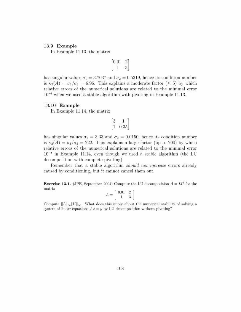
13.9 ExampleIn Example 11.13, the matrix[

0.01 21 3

]has singular values σ1 = 3.7037 and σ2 = 0.5319, hence its condition numberis κ2(A) = σ1/σ2 = 6.96. This explains a moderate factor (≤ 5) by whichrelative errors of the numerical solutions are related to the minimal error10−t when we used a stable algorithm with pivoting in Example 11.13.

13.10 ExampleIn Example 11.14, the matrix[

3 11 0.35

]has singular values σ1 = 3.33 and σ2 = 0.0150, hence its condition numberis κ2(A) = σ1/σ2 = 222. This explains a large factor (up to 200) by whichrelative errors of the numerical solutions are related to the minimal error10−t in Example 11.14, even though we used a stable algorithm (the LUdecomposition with complete pivoting).

Remember that a stable algorithm should not increase errors alreadycaused by conditioning, but it cannot cancel them out.

Exercise 13.1. (JPE, September 2004) Compute the LU decomposition A = LU for thematrix

A =

[0.01 2

1 3

]Compute ‖L‖∞‖U‖∞. What does this imply about the numerical stability of solving asystem of linear equations Ax = y by LU decomposition without pivoting?

108

Chapter 14

Numerically Stable Least Squares

In Chapter 10 we discussed overdetermined systems of equations

Ax ≈ b

where A ∈ Cm×n with m ≥ n and presented three algorithms for computingthe least squares solution x: (i) based on normal equations, (ii) based on QRdecomposition, and (iii) based on SVD.

14.1 Normal equations revisitedAlgorithm 10.9 via normal equations has many advantages. It is the

simplest and most elegant algorithm for the least squares problem. It shouldbe used whenever the computations are precise, in particular if one solvesthe problem manually (on paper).

For machine computations, algorithm 10.9 seems to be good, too: it is atleast twice as cheap (in terms of flops) as the other two algorithms, so it is thefastest one. It has been used in computer programming almost exclusivelybefore 1970s, when computers were slow and the top speed was high priority.

However, machine computations involve round-off errors. And it hasbeen gradually noticed that Algorithm 10.9 based on normal equations tendsto magnify errors and produce inaccurate results to the extent that waseventually deemed unacceptable. As of now, normal equations are almostentirely abandoned and used only to demonstrate how bad things can be.

The loss of accuracy can be best understood in terms of the conditionnumber. If A is the given matrix, then we have seen (Section 12.14) that

κ2(A∗A) = [κ2(A)]2.

If the matrix A is ill-conditioned (i.e., its condition number is large), thenthe matrix A∗A will have a much larger condition number.

More precisely, suppose that our machine arithmetic has precision u =10−p (defined in Section 11.11) and let κ2(A) ∼ 10q for some q > 0. Then a

109

numerical solution of the least squares problem should produce p−q accuratedecimal digits. However, solving the problem by normal equations wouldinvolve the matrix A∗A whose condition number is

κ2(A∗A) = [κ2(A)]2 ∼ 102q.

Thus the resulting numerical solution would have only p−2q accurate decimaldigits: we lose an extra q accurate digits.

Such a loss of accuracy may be disastrous. Suppose we use single precision(p = 7) and our matrix A is just mildly ill-conditioned, with κ2(A) ∼ 103

(recall Section 12.9). Then solving the problem via normal equations wewould give us just 7 − 2 · 3 = 1 (one!) accurate digit, instead of 7 − 3 = 4that can be theoretically expected for the given matrix.

Another extreme example: suppose

A =

1 1ε 00 ε

where ε ≈ 1

2

√u. This matrix has condition number

κ2(A) =

√2 + ε2

ε≈ 2

ε,

so we can expect the numerical solution to have relative error ∼ u/ε ∼√

u,which is not too bad (in single precision we expect 3-4 accurate digits, andin double precision – eight accurate digits).

However, normal equations require the construction of the matrix

A∗A =

[1 + ε2 1

1 1 + ε2

]Since ε2 < u, the matrix A∗A will be stored in the computer memory as [ 1 1

1 1 ](the additional term ε2 would disappear due to round-off; recall Section 12.9).The matrix [ 1 1

1 1 ] is singular, so the algorithm via normal equations would justfail (the computer program would crush).

Still, it is possible to find a reasonably good numerical solution in the lastexample, with relative error ∼

√u, if one uses more elaborate algorithms.

110

14.2 QR-based algorithm revisitedLet us examine the accuracy of the QR-based Algorithm 10.10.Due to Section 12.11 (part 4), κ2(A) = κ2(QA) for any unitary matrix

Q ∈ Cm×m, henceκ2(R) = κ2(Q∗A) = κ2(A).

Therefore, this method is safe, regarding the conditioning of the problem, noadditional loss of accuracy occurs due to conditioning.

The other aspect of numerical algorithms is stability, described in Chap-ter 13. The actual error may greatly depend on a particular sequence ofcomputations producing the matrices Q and R.

So far we have mentioned two specific procedures for constructing Q andR: the classical Gram-Schmidt (Sect. 1.25) and the modified Gram-Schmidt(Sect. 9.10). It turns out that the classical Gram-Schmidt is unstable, henceit leads to unpredictable round-off errors in numerical computations. Themodified Gram-Schmidt is stable and generally produces accurate results(see programming assignment).

However, there are better algorithms for computing the QR decomposi-tion: those are based on reflection and rotation matrices. We will learn themin this chapter.

14.3 SVD-based algorithm revisitedLastly we briefly examine the accuracy of the SVD-based Algorithm 10.11.Let A = UDV ∗ be an SVD of A. Due to Section 12.11 (part 4), κ2(A) =

κ2(UA) = κ2(AV ) for any unitary matrices U ∈ Cm×m and V ∈ Cn×n hence

κ2(D) = κ2(U∗AV ) = κ2(A).

Therefore, this method is just as safe, regarding the conditioning of theproblem, as the QR-based Algorithm 10.10.

However, Algorithm 10.11 requires the computation of an SVD for thematrix A, for which no simple algorithm exists (the computation of SVD isbeyond the scope of this course). Standard software packages (like MATLAB)use only stable and highly accurate algorithms for the SVD computation. Ifone uses a standard software package, the SVD-based method 10.11 is asgood as the QR-based method 10.10 (see programming assignment).

Just a minor note: the SVD-based method 10.11 is more reliable whenthe matrix A is almost singular or exactly singular; cf. Section 10.12.

111

14.4 HyperplanesLet V be a finite dimensional vector space. A subspace W ⊂ V is called a

hyperplane if dimW = dimV −1. If V is an inner product space and W ⊂ Va hyperplane, then

dimW⊥ = 1.

If x ∈ W⊥ is a nonzero vector, then W⊥ = span{x}. In that case

W =(W⊥)⊥ =

(span{x}

)⊥.

Hence any hyperplane W is completely determined by a non-zero vector xorthogonal to it.

14.5 ReflectionsLet W ⊂ V be a hyperplane in an inner product space V . Recall that

V = W ⊕W⊥ (Sect. 1.29). Thus for any vector v ∈ V we have a uniquedecomposition v = w + w′, where w ∈ W and w′ ∈ W⊥.

The linear operator P on V defined by

Pv = P (w + w′) = w − w′

is called a reflection (or reflector) across the hyperplane W .

Ww

vw′

x

P (v)−w′

Note: P (w) = w for all w ∈ W , so P is an identity on W . Also, P (w′) = −w′ for allw′ ∈W⊥, so P negates vectors orthogonal to W .

Since W is completely determined by a nonzero vector x orthogonal to W , the reflector

can be fully described in terms of x.

14.6 Householder reflection matricesLet x 6= 0 be a nonzero vector in Cn. The n× n matrix

P = I − 2xx∗

x∗x= I − 2

xx∗

‖x‖2

is called the Householder reflection matrix (or Householder reflector) corre-sponding to x.

Obviously, P is unchanged if x is replaced by cx for any c 6= 0.

112

14.7 Basic properties of Householder reflectorsLet P be the reflector matrix corresponding to a vector x 6= 0. Then

(a) Px = −x.

(b) Py = y whenever 〈y, x〉 = 0.

(c) P is Hermitian (in the real case it is symmetric).

(d) P is unitary (in the real case it is orthogonal).

(e) P is involution, i.e. P 2 = I.

Proof. Direct calculation. �

14.8 TheoremLet y ∈ Cn. Choose a scalar σ ∈ C so that

|σ| = ‖y‖ and σ · 〈e1, y〉 ∈ R. (14.1)

Suppose that x = y+ σe1 6= 0. Let P = I − 2xx∗/‖x‖2 be the correspondingHouseholder reflector. Then Py = −σe1.

Proof. By direct calculation, we have

〈y − σe1, y + σe1〉 = ‖y‖2 − σ〈e1, y〉+ σ〈y, e1〉 − |σ|2 = 0

where we used both identities of (14.1). Now

14.7(a) implies: P (y + σe1) = −y − σe1

14.7(b) implies: P (y − σe1) = y − σe1

Adding these two equations proves the theorem. �

14.9 Remarks

(a) To choose σ in Theorem 14.8, write a polar representation for 〈e1, y〉 = reiθ andthen set σ = ±‖y‖e−iθ.

(b) In the real case, we have 〈e1, y〉 ∈ R, and one can just set σ = ±‖y‖. For machinecalculation with round-off errors, the better choice is

σ =

{+‖y‖ if 〈e1, y〉 ≥ 0

−‖y‖ if 〈e1, y〉 < 0.

Then the computation of the vector x = y + σe1 will be numerically stable, therewill be no danger of catastrophic cancelation.

113

(c) It is geometrically obvious that for any two vectors x, y ∈ Rn with equal 2-norms,‖x‖2 = ‖y‖2, there is a reflector P that takes x to y. In the complex space Cn, thisis not true: for generic vectors x, y ∈ Cn with equal 2-norms there is no reflectorthat takes x to y. But according to Theorem 14.8, one can always find a reflectorthat takes x to cy with some scalar c ∈ C.

14.10 CorollaryFor any vector y ∈ Cn there is a scalar σ (which was defined in 14.8 and

specified in 14.9) and a matrix P , which is either a reflector or the identity(P = I), such that Py = −σe1.

Proof. Apply Theorem 14.8 in the case y + σe1 6= 0 and set P = I otherwise. �

14.11 QR Decomposition via Householder reflectorsFor any A ∈ Cm×n with m ≥ n there is a QR decomposition with a

unitary matrix Q ∈ Cm×m that is a product of Householder reflectors. Thenumber of those reflectors is ≤ n.

Proof. We use induction on n. Let n = 1, so that A is just one column m-vector. ByCorollary 14.10 there is a matrix P (a reflector or identity) such that PA = −σe1 witha scalar σ ∈ C. Hence, A = PR where R = −σe1 is am upper triangular matrix m × 1.This provides the basis for our induction.

Now let n ≥ 1. Let a1 denote the first column of A. Again, by Corollary 14.10 thereis a matrix P (a reflector or identity) such that Pa1 = −σe1. Hence,

PA =

[−σ w∗

0 B

]where w ∈ Cn−1 and B ∈ C(m−1)×(n−1). By the inductive assumption, there is a unitarymatrix Q1 ∈ C(m−1)×(m−1) and an upper triangular matrix R1 ∈ C(m−1)×(n−1) such thatB = Q1R1. Now we expand Q1 to a unitary m×m matrix as follows:

Q2 =

[1 00 Q1

]By Section 2.11, the matrix Q2 is unitary whenever Q1 is. Furthermore, if Q1 is a productof≤ n−1 reflectors, then the same is true forQ2. Now one can easily check that PA = Q2Rwhere

R =

[−σ w∗

0 R1

]is an upper triangular matrix. Hence, A = QR with Q = PQ2. �

114

14.12 Givens rotation matricesLet 1 ≤ p < q ≤ m and θ ∈ [0, 2π). The matrix G = Gp,q,θ defined by

gpp = cos θ, gpq = sin θ, gqp = − sin θ, gqq = cos θ,

and gij = δij otherwise is called a Givens rotation matrix (or Givens rotator):

G =

1. . .

1c s

1. . .

1−s c

1. . .

1

← p

← q

↑ ↑

p q

(here we use convenient shorthand notation c = cos θ and s = sin θ).

It is easy to check that G is an orthogonal matrix (recall Sect. 2.11).

14.13 Geometric description of Givens rotatorsNote that the vector y = Gx has components

yp = xp cos θ + xq sin θ

yq = −xp sin θ + xq cos θ

yi = xi ∀ i /∈ {p, q}

Hence the matrix G defines a clockwise rotation through the angle θ of thexpxq coordinate plane in Rm with all the other coordinates left unchanged.

115

14.14 QR decomposition via Givens rotatorsFor any A ∈ Rm×n with m ≥ n there is a QR decomposition with an

orthogonal matrix Q ∈ Rm×m that is a product of Givens rotators.

Proof. Let ap be the leftmost column of A that contains a nonzero entry below the maindiagonal, i.e.,

p = min{j ≥ 1: aij 6= 0 for some i > j}

(if such p does not exist, the matrix A is already upper triangular).Let aqp 6= 0 be one of the nonzero entries in the column ap below the main diagonal,

i.e., satisfying q > p. Consider the matrix A′ = GA where G = Gp,q,θ is a Givens rotator.Note that p and q are already selected, but we are still free to choose θ.

The structure of the matrices A = (aij) and A′ = (a′ij) can be revealed by examiningthe following diagram:

1. . .

1c s

1. . .

1−s c

1. . .

1

∗ · · ·

0. . .

0 0 ∗ ∗0 · · · 0 app0 · · · 0 ∗...

. . ....

...0 · · · 0 ∗0 · · · 0 aqp0 · · · 0 ∗...

. . ....

...0 · · · 0 ∗ · · ·

=

∗ · · ·

0. . .

0 0 ∗ ∗0 · · · 0 a′pp0 · · · 0 ∗...

. . ....

...0 · · · 0 ∗0 · · · 0 a′qp0 · · · 0 ∗...

. . ....

...0 · · · 0 ∗ · · ·

The following facts can be verified by direct inspection:

(a) The first p − 1 columns of A′ are the same as those of A, hence they are still zerobelow the main diagonal.

116

(b) In the p-th column, only the components a′pp and a′qp will be different from thecorresponding components of A (hence, if A had some zeros in the p-th columnbelow the main diagonal, those will propagate to A′).

(c) The subdiagonal component a′qp of A′ is given by

a′qp = −app sin θ + aqp cos θ.

Our goal is to make a′qp = 0. We can achieve this by using our freedom to choose θ. Thefollowing choice will do it:

cos θ =app√

a2pp + a2

qp

and sin θ =aqp√

a2pp + a2

qp

. (14.2)

Note that one never actually evaluates the angle θ, since Gp,q,θ only contains cos θ andsin θ, and these are given by the above formulas.

In this way we eliminate one nonzero element aqp below the main diagonal. Working

from left to right, one can convert A into an upper triangular matrix GA = R where

G = Gpk,qk,θk · · ·Gp1,q1,θ1

will be a product of Givens rotators. Each nonzero element of A below the main diagonalrequires one multiplication by a rotator. Then we get A = QR with an orthogonal matrix

Q = GT = GTp1,q1,θ1 · · ·GTpk,qk,θk

.

It remains to note that GTp,q,θ = Gp,q,−θ, so it is a Givens rotator, too. �

14.15 Cost of QR via Givens rotatorsThe evaluation of cos θ and sin θ by (14.2) takes 6 flops (the square root

extraction is counted here as one flop). The subsequent multiplication of Aby Gp,q,θ takes 6n flops. Thus, the elimination of one nonzero subdiagonalcomponent of A takes 6n+6 flops. If A originally has k nonzero subdiagonalentries, the QR decomposition via Givens rotators will take 6k(n+ 1) ∼ 6knflops.

When the lower triangle of A is mostly filled with nonzero numbers, thenk is close to its maximal value, mn−n2/2. In that case the total cost will bevery high, it will greatly exceed the cost of QR via Householder reflectors.Hence Givens rotators are very inefficient for generic matrices.

However, Givens rotators work well if the matrix A is sparse, i.e., con-tains just a few nonzero components below the main diagonal. Then Givensrotators can give the quickest result. We will see such instances later.

117

Exercise 14.1. Let x, y ∈ Cn be such that x 6= y and ‖x‖2 = ‖y‖2 6= 0. Show that thereis a reflector matrix P such that Px = y if and only if 〈x, y〉 ∈ R. For an extra credit:show that if the above reflector exists, then it is unique.

Exercise 14.2. (simplified of JPE, May 2011) Prove that any Givens rotator matrix inR2 is a product of two Householder reflector matrices. Can a Householder reflector matrixbe a product of Givens rotator matrices?

Exercise 14.3 (Bonus). (JPE May, 2010) Let

A =

3 −30 44 1

(a) Find the QR factorization of A by Householder reflectors.

(b) Use the results in (a) to find the least squares solution of Ax = b, where

b = [16 11 17]T

(Note: there is a typo in the original JPE exam, it is corrected here.)

118

Chapter 15

Computation of Eigenvalues: Theory

15.1 PrefaceEigenvalues of a matrix A ∈ Cn×n are the roots of its characteristic poly-

nomialCA(x) = det(xI − A), where degCA(x) = n.

It is a consequence of the famous Galois group theory (Abel’s theorem) thatthere is no closed formula for the roots of a generic polynomial of degree> 4. Hence, there are no finite algorithms for computation of the roots ofpolynomials (or eigenvalues, for that matter).

Thus, all the methods for computing eigenvalues of matrices of size n ≥5 are necessarily iterative, they provide successive approximations to theeigenvalues, but never exact results. Furthermore, even though for n = 3 andn = 4 exact formulas exist, they are rather impractical and often numericallyunstable, so even in these cases iterative methods are used instead.

For this reason, matrix decompositions that reveal eigenvalues (Schurand SVD) cannot be implemented by finite algorithms. On the other hand,decompositions that do not reveal eigenvalues (QR, LU, Cholesky) can beimplemented by finite algorithms (and we have seen some of those):

Decompositions Decompositions

revealing eigenvalues not revealing eigenvalues

SVDLU

SchurCholesky

QR

No finite Finite

algorithms exist algorithms exist

In the last chapters of the course we will learn iterative algorithms forcomputing eigenvalues and eigenvectors. We note that the most important

119

matrix decomposition, SVD, requires the eigenvalues of a Hermitian posi-tive semidefinite matrix A∗A. Hence it is particularly important to developalgorithms for computing eigenvalues of Hermitian matrices.

If an eigenvalue λ of a matrix A is known, an eigenvector x correspondingto λ can be found by solving the linear system (A − λI)x = 0 (say, by LUdecomposition). Conversely, if an eigenvector x is known, the correspondingeigenvalue λ can be immediately found by simple formula λ = (Ax)i/xi,whenever xi 6= 0. Thus eigenvalues help to compute eigenvectors and viceversa. For this reason eigenvalues and eigenvectors are often computed ‘inparallel’. In this chapter, we develop a theoretical basis for computation ofeigenvalues and eigenvectors, while in the next two chapters we will turn topractical algorithms.

15.2 Rayleigh quotientLet A ∈ Cn×n. We call

r(x) =x∗Ax

x∗x=〈Ax, x〉〈x, x〉

, x 6= 0

the Rayleigh quotient of x.

15.3 Restriction to the unit sphereThe Rayleigh quotient is defined for all vectors x 6= 0, so it is a function

on Cn \ {0}, with values in C. However, for any nonzero scalar c 6= 0

r(cx) =〈cAx, cx〉〈cx, cx〉

=|c|2〈Ax, x〉|c|2〈x, x〉

=〈Ax, x〉〈x, x〉

= r(x),

hence r is constant on the line span{x}. Since any nonzero vector x 6= 0 isa scalar multiple of a unit vector u = x/‖x‖, the function r(x) is completelydefined by its values on the unit sphere (1.1)

S1 = {u ∈ Cn : ‖u‖ = 1}.

On the unit sphere S1 the Rayleigh quotient can be computed by a simplerformula:

r(u) = u∗Au = 〈Au, u〉.

Note that r(u) is a quadratic function of the coordinates of u ∈ S1.

120

15.4 Properties of Rayleigh quotient

(a) If A is Hermitian, then r(x) ∈ R for any nonzero vector x ∈ Cn.[This follows from Section 4.12(a)]

(b) If x is an eigenvector with eigenvalue λ, then Ax = λx and so

r(x) = λ

(c) If x is an arbitrary unit vector, then r(x)x = (x∗Ax)x is the orthogonalprojection of the vector Ax onto the line spanned by x. Hence

‖Ax− r(x)x‖2 = minµ∈C‖Ax− µx‖2

Note: if one regards x as an ‘approximate’ eigenvector, then the Rayleighquotient r(x) is the best choice that one can make for the associated ‘ap-proximate’ eigenvalue in the sense that the value µ = r(x) comes closest (inthe 2-norm) to achieving the desired relation Ax− µx = 0.

Let A ∈ Cn×n and x a unit eigenvector of A corresponding to eigenvalue λ. Let y ≈ x be

another unit vector close to x and r = y∗Ay. It follows from the above that r ≈ λ, but

how close is r to λ?

15.5 TheoremLet A ∈ Cn×n and x a unit eigenvector of A corresponding to eigenvalue

λ. Let y be another unit vector and r = y∗Ay. Then

|λ− r| ≤ 2 ‖A‖2 ‖x− y‖2. (15.1)

Moreover, if A is a Hermitian matrix, then there is a constant C = C(A) > 0such that

|λ− r| ≤ C ‖x− y‖22. (15.2)

Proof. To prove (15.1), we write

λ− r = x∗A(x− y) + (x− y)∗Ay.

Now the triangle inequality and Cauchy-Schwarz inequality readily give (15.1).

121

Now, assume that A is Hermitian. Then there is an ONB of eigenvectors, and we canassume that x is one of them. Denote that ONB by {x, x2, . . . , xn} and the correspondingeigenvalues by λ, λ2, . . . , λn. Let y = cx+ c2x2 + · · ·+ cnxn. Then

‖y − x‖2 = |c− 1|2 +

n∑i=2

|ci|2 ≥n∑i=2

|ci|2

On the other hand, ‖y‖ = 1, i.e., c2 + c22 + · · ·+ c2n = 1, so

λ = λ|c|2 +

n∑i=2

λ|ci|2

Now, Ay = cλx+∑ni=2 ciλixi, therefore

r = 〈Ay, y〉 = λ|c|2 +

n∑i=2

λi|ci|2.

Subtracting the last two formulas gives

λ− r =

n∑i=2

(λ− λi)|ci|2.

The result now follows withC = max

2≤i≤n|λ− λi|.

The theorem is proved. �

Note: one may feel uncomfortable to deal with an unspecified constant C in(15.2). In fact, it easily follows from Sect. 4.20 that C ≤ 2‖A‖2.

15.6 LemmaLet L and G be subspaces of Cn and dimG > dimL. Then there is a

nonzero vector y ∈ G orthogonal to L, i.e., y ∈ L⊥.

Proof. By way of contradiction, suppose G∩L⊥ = {0}. Then G⊕L⊥ would be a subspaceof Cn, and its dimension would be

dimG+ dimL⊥ = dimG+ n− dimL > n,

which is impossible. �

Next let A ∈ Cn×n be a Hermitian matrix with eigenvalues λ1, . . . , λn. Sincethey are all real, we can number them in an increasing order, so that

λ1 ≤ · · · ≤ λn.

Also recall that x∗Ax ∈ R for any vector x ∈ C, by Sect. 15.4 (a).

122

15.7 Courant-Fisher Minimax TheoremLet A ∈ Cn×n be a Hermitian matrix with eigenvalues λ1 ≤ · · · ≤ λn.

Then for every i = 1, . . . , n

λi = minL : dimL=i

maxx∈L\{0}

x∗Ax

x∗x

where L stands for a vector subspace of Cn.

Proof. Let {u1, . . . , un} be an ONB of eigenvectors of A corresponding to theeigenvalues λ1, . . . , λn. If dimL = i, then by Lemma 15.6 there is a nonzerovector y ∈ L \ {0} orthogonal to the space span{u1, . . . , ui−1}. Hence, thefirst i− 1 coordinates of y are zero, i.e. y =

∑nj=i cjuj. Thus

y∗Ay

y∗y=

∑nj=i |cj|2λj∑nj=i |cj|2

≥ λi

because λj ≥ λi for all j = i, . . . , n. Therefore,

maxx∈L\{0}

x∗Ax

x∗x≥ y∗Ay

y∗y≥ λi.

On the other hand, let Li = span{u1, . . . , ui}. Obviously, dimLi = i and forevery nonzero vector x ∈ Li we have x =

∑ij=1 cjuj, so

x∗Ax

x∗x=

∑ij=1 |cj|2λj∑ij=1 |cj|2

≤ λi

because λj ≤ λi for all j = 1, . . . , i. The theorem is proved. �

15.8 CorollaryA close examination of the proof of the above theorem gives us

λi = maxx∈Li\{0}

x∗Ax

x∗x, (15.3)

where Li = span{u1, . . . , ui}.

123

15.9 TheoremLet A and ∆A be two Hermitian matrices. Let α1 ≤ · · · ≤ αn be the

eigenvalues of A. Let δmin and δmax the smallest and the largest eigenvaluesof ∆A. Denote the eigenvalues of the matrix B = A+ ∆A by β1 ≤ · · · ≤ βn.Then for each i = 1, . . . , n

αi + δmin ≤ βi ≤ αi + δmax. (15.4)

Proof. Let {u1, . . . , un} be an ONB of eigenvectors of A corresponding toits eigenvalues α1, . . . , αn. For each i = 1, . . . , n, let Li = span{u1, . . . , ui}.Then dimLi = i, hence by Theorem 15.7 and Corollary 15.8

βi ≤ maxx∈Li\{0}

x∗Bx

x∗x

= maxx∈Li\{0}

[x∗Ax

x∗x+x∗∆Ax

x∗x

]≤ max

x∈Li\{0}

x∗Ax

x∗x+ max

x∈Li\{0}

x∗∆Ax

x∗x

= αi + maxx∈Li\{0}

x∗∆Ax

x∗x

≤ αi + maxx∈Cn\{0}

x∗∆Ax

x∗x

= αi + δmax

where at the last step we used Section 4.12 (b). Thus we proved the rightinequality in (15.4). The left one can be proved by a similar calculation, butwe can achieve the result quicker by a trick. We can rewrite that inequalityas

αi ≤ βi − δmin (15.5)

and note that −δmin is the largest eigenvalue of the matrix −∆A. Then weapply the (already proven) right inequality in (15.4) to the matrices B, −∆Aand A = B + (−∆A) and obtain (15.5). The theorem is completely proved.�

15.10 CorollarySince ‖∆A‖2 = max{|δmin|, |δmax|} (due to Section 4.20), we have

|αi − βi| ≤ ‖∆A‖2 ∀i = 1, . . . , n

124

15.11 Approximation analysis using the residualSuppose one finds an approximate eigenvalue µ and an approximate unit eigenvector

x of a matrix A. How can one estimate the closeness of µ to the actual (but unknown)eigenvalue λ of A?

One way to do this is to compute the residual r = Ax − µx. If r = 0, then µ is aneigenvalue of A. If that r is small, then one may hope that µ is close to an eigenvalue ofA. But how close is it?

To place this question in the context of the previous theorems, we define the matrix∆A = −rx∗. Then

(A+ ∆A)x = Ax− rx∗x = µx,

so (µ, x) are an exact (!) eigenpair of the perturbed matrix A + ∆A. Also note that‖∆A‖2 = ‖r‖2, so the norm ‖∆A‖2 is readily computable.

If we could apply Corollary 15.10, we would be able to conclude that

|µ− λ| ≤ ‖∆A‖2 = ‖r‖2. (15.6)

But! In Corollary 15.10 the matrices A and ∆A must be Hermitian. And our matrices

(especially ∆A = −rx∗) may not be Hermitian. Thus we need to extend the estimate in

Corollary 15.10 to more general matrices.

15.12 Bauer-Fike theoremLet A ∈ Cn×n be a diagonalizable matrix, so that

X−1AX = D = diag{λ1, . . . , λn}

If µ is an eigenvalue of a perturbed matrix A+ ∆A, then

min1≤i≤n

|µ− λi| ≤ κp(X) ‖∆A‖p

where ‖ · ‖p stands for any p-norm (1 ≤ p ≤ ∞).

Proof. The matrix A+ ∆A− µI is singular. Hence so is the matrix

X−1(A+ ∆A− µI)X = D +X−1∆AX − µI.

If D − µI is singular, then µ is an eigenvalue of A and the claim is trivial. Otherwise

(D − µI)−1[D +X−1∆AX − µI

]= I + (D − µI)−1(X−1∆AX)

is a singular matrix. The Neumann lemma (Exercise 1.2) implies

1 ≤ ‖(D − µI)−1(X−1∆AX)‖p ≤ ‖(D − µI)−1‖p‖X−1‖p‖∆A‖p‖X‖p

Lastly, observe that (D − µI)−1 is diagonal, so

‖(D − µI)−1‖p = max1≤i≤n

1

|λi − µ|=

1

min1≤i≤n |λi − µ|

The theorem now follows. �

125

15.13 CorollaryIf A is a normal matrix, then in the above theorem

min1≤i≤n

|µ− λi| ≤ ‖∆A‖2

because X is a unitary matrix and so κ2(X) = 1. Thus, (15.6) is actually true

for any normal matrix, in particular for any Hermitian matrix A.

Theorem 15.12 answers the question raised in Section 15.11, it gives an estimate

on |µ− λ| in terms of ‖∆A‖p and κp(X). However, this answer may not be good

enough – it gives one estimate for all eigenvalues. In practical applications, some

eigenvalues can be estimated better than others. It is important then to develop

finer estimates for individual eigenvalues.

15.14 Left eigenvectors (definition)Let A ∈ Cn×n. A nonzero vector x ∈ Cn is called a left eigenvector of A

corresponding to an eigenvalue λ if

x∗A = λx∗

Note: this is equivalent toA∗x = λx,

i.e., x is an ordinary (“right”) eigenvector of A∗ corresponding to the eigenvalue λ:

(λ, x) is a left eigenpair for A ⇐⇒ (λ, x) is a right eigenpair for A∗. (15.7)

But why don’t we introduce a notion of left eigenvalue?

15.15 LemmaA matrix A has a left eigenvector x 6= 0 corresponding to eigenvalue λ if

and only if λ is a root of the characteristic polynomial of A:

(λ, x) is a left eigenpair for A ⇐⇒ (λ, y) is a right eigenpair for A for some y 6= 0

Proof. A∗x = λx can be written as (A∗ − λI)x = 0, and since x 6= 0, we conclude that

det(A∗ − λI) = 0. Due to (0.3), we have det(A− λI) = 0, i.e., CA(λ) = 0. �

Lemma 15.15 explains why we do not introduce a notion of left eigenvalue: theset of eigenvalues for left eigenvectors is just the same as the set of eigenvalues forordinary (right) eigenvectors.

Our next question is: for a given eigenvalue λ of A, how different the corre-

sponding left and right eigenvectors are? More precisely, how different the corre-

sponding left and right eigenspaces are?

126

15.16 LemmaFor any eigenvalue λ of A, the dimension of the right eigenspace equals

the dimension of the left eigenspace (i.e., the geometric multiplicity of λ isthe same, in the left and right senses).

Proof. Recall that the ordinary (right) eigenspace is Ker(A − λI). By (15.7), the lefteigenspace is Ker(A∗ − λI). Now we have, due to (0.1):

dim Ker(A− λI) = n− rank(A− λI) = n− rank(A∗ − λI) = dim Ker(A∗ − λI).

We used the fact that rankB = rankB∗ for any matrix B. �

Lemma 15.16 shows that for each eigenvalue λ of A the corresponding left andright eigenspaces have the same dimension. But do those spaces have to coincide?If not, do they have to be close to each other?

When both eigenspaces are one-dimensional and real, their closeness can bemeasured by the angle between them. If x is a right unit eigenvector and y is a leftunit eigenvector, then the angle θ between the corresponding eigenspaces span(x)and span(y) satisfies cos θ = 〈x, y〉; cf. (1.22). Thus the “indicator of closeness” ofthose eigenspaces will be the inner product 〈x, y〉 = y∗x.

Recall that by Cauchy-Schwarz inequality (Section 1.12) for any unit vectors

x and y we have |〈x, y〉| ≤ 1, so the range of values of |〈x, y〉| is the interval [0, 1].

The angle between the left and right eigenspaces span(x) and span(y) is small if

|〈x, y〉| is close to 1, and large if |〈x, y〉| is close to 0. These spaces coincide if

|〈x, y〉| = 1 and are orthogonal to each other if |〈x, y〉| = 0.

xy

θ small

|〈x, y〉| ≈ 1

x

y

θ large

|〈x, y〉| ≈ 0

x

y

θ = π/2

|〈x, y〉| = 0

y

x

θ = 0

|〈x, y〉| = 1

15.17 LemmaLet λ be an eigenvalue with a right eigenvector x, and µ 6= λ be another

eigenvalue with a left eigenvector y. Then 〈x, y〉 = 0, i.e. x ⊥ y.

(In other words, left and right eigenspaces corresponding to different eigenval-

ues are orthogonal to one another.)

Proof. First, we have 〈Ax, y〉 = λ〈x, y〉. On the other hand, according to (15.7), we have

〈Ax, y〉 = 〈x,A∗y〉 = 〈x, µy〉 = µ〈x, y〉.

Hence, λ〈x, y〉 = µ〈x, y〉. Since λ 6= µ, we must have 〈x, y〉 = 0. �

127

15.18 LemmaLet λ be a simple eigenvalue (this means its algebraic multiplicity is one)

with right and left eigenvectors x and y, respectively. Then 〈x, y〉 6= 0.

(In other words, left and right eigenspaces corresponding to the same simple

eigenvalue λ cannot be orthogonal to each other.)

Proof. We can always choose unit eigenvectors, in particular let ‖x‖ = 1. By the Schurdecomposition (Section 6.1), there is a unitary matrix Q such that

Q∗AQ =

[λ h∗

0 B

]with some h ∈ Cn−1 and B ∈ C(n−1)×(n−1). According to the proof in Section 6.1, we canconstruct the matrix Q so that its first column is the vector x, i.e., that Qe1 = x. Sinceλ is a simple eigenvalue of A, it cannot be an eigenvalue of B. Thus the matrix λI −B isinvertible. Hence λI −B∗ is invertible, too. Denote z = (λI −B∗)−1h. Then

λz −B∗z = h =⇒ h∗ + z∗B = λz∗.

Now one can readily verify that

[ 1 z∗]Q∗AQ = λ [ 1 z∗] =⇒ [ 1 z∗]Q∗A = λ [ 1 z∗]Q∗.

Denote w∗ = [ 1 z∗]Q∗. The above equation now takes a short form

w∗A = λw∗.

Hence w is a left eigenvector of A. By the simplicity of λ, the vector w is a nonzeromultiple of y. However, observe that

w∗x = [ 1 z∗]Q∗Qe1 = [ 1 z∗] e1 = 1 ( 6= 0),

which proves the lemma. �

15.19 TheoremLet A ∈ Cn×n have a simple eigenvalue λ with right and left unit eigen-

vectors x and y, respectively. Let E ∈ Cn×n be another matrix such that‖E‖2 = 1. For small ε, denote by λ(ε), x(ε), and y(ε) the eigenvalue, theright and left unit eigenvectors of the matrix A + εE that correspond to λ,x and y when ε = 0. Then

|λ′(0)| ≤ 1

|y∗x|

128

Proof. We note that the existence and differentiability of λ(ε), x(ε), and y(ε) follow fromthe inverse function theorem; we leave out the details. Now we write the equation

(A+ εE)x(ε) = λ(ε)x(ε)

and differentiate it with respect to ε:

Ax′(ε) + Ex(ε) + εEx′(ε) = λ′(ε)x+ λx′(ε)

Setting ε = 0 givesAx′(0) + Ex = λ′(0)x+ λx′(0).

Now we premultiply this equation by the vector y∗:

y∗Ax′(0) + y∗Ex = λ′(0)y∗x+ λ y∗x′(0).

Since y∗A = λy∗, the two terms with x′(0) cancel each other out, and we arrive at

y∗Ex = λ′(0) y∗x.

Now we use the Cauchy-Schwarz inequality and other standard inequalities:

|λ′(0)| |y∗x| = |y∗Ex| = |〈Ex, y〉| ≤ ‖Ex‖2 ‖y‖2 ≤ ‖E‖2 ‖x‖2 ‖y‖2 = 1.

This proves the theorem. Note that y∗x 6= 0 by Lemma 15.18. �

We regard the matrix A + εE as the perturbation of A “in the direction” ofE. If the matrix E is known, one can find λ′(0) exactly:

λ′(0) =y∗Ex

y∗x.

Knowing λ′(0) would be useful, because by Taylor expansion

λ(ε) = λ+y∗Ex

y∗xε+O(ε2)

we could have a fairly good approximation to λ(ε) for small ε. In practice, how-ever, the perturbation matrix E is totally unknown, we only know the order ofmagnitude of perturbation, i.e., the value of ε. Hence we cannot compute an ap-proximation to λ(ε) by Taylor expansion, we can only use the upper bound ofTheorem 15.19 to estimate how far λ(ε) can be from λ:

|λ(ε)− λ(0)| ≤ ε

|y∗x|+O(ε2).

This shows that the sensitivity of the eigenvalue λ to small perturbations of the

matrix A is determined by the value of 1|y∗x| .

129

15.20 Condition number of a simple eigenvalueLet λ be a simple eigenvalue (this means that its algebraic multiplicity is

equal to one) of a matrix A ∈ Cn×n and x, y the corresponding right and leftunit eigenvectors. Then

K(λ) =1

|y∗x|is called the condition number of the eigenvalue λ.

15.21 Remarks

(a) The condition number K(λ) is well defined for every simple eigenvalue.Indeed, by Lemma 15.18 we have |y∗x| 6= 0. Also, the value of |y∗x| doesnot depend on the particular choice of x and y, because |(ay)∗(bx)| =|ab| |y∗x| = |y∗x| for any scalars a and b such that |a| = |b| = 1.

(b) If λ is a multiple eigenvalue, the condition number K(λ) is not defined,and for a good reason. If the geometric multiplicity of λ is ≥ 2, then forany right eigenvector x there is a left eigenvector y such that y∗x = 0(Exercise 15.4), which would result in K(λ) =∞.

(c) Even if the geometric multiplicity of λ equals one, we may have apathological situation where y∗x = 0. Example: A = [ 0 1

0 0 ] with amultiple eigenvalue λ = 0; here the right eigenvector is x = [ 1

0 ] and theleft eigenvector is y = [ 0

1 ].

15.22 Properties of condition numbers for simple eigenvalues

(a) K(λ) ≥ 1.

(b) If the matrix A is normal, then K(λ) = 1 for all its simple eigenvalues.

(c) Conversely, if a matrix A has all simple eigenvalues with K(λ) = 1 foreach of them, then A is normal.

Proof. By Cauchy-Schwarz inequality, |y∗x| ≤ ‖x‖2‖y‖2 = 1. This implies (a). For the

proofs of (b) and (c), see Exercises 15.2 and 15.3.

130

15.23 Relation to Schur decompositionWe see that matrices with the most well-conditioned eigenvalues (such

that K(λ) = 1 for all the eigenvalues) are normal matrices. On the otherhand, normal matrices are characterized by the fact that their Schur decom-position Q∗AQ = T results in an upper-triangular matrix T that is actuallydiagonal (i.e., its off-diagonal components are zeros). One can expect that ifthe Schur matrix T is nearly diagonal (i.e., its off-diagonal components aresmall), then the eigenvalues of A are well-conditioned. On the contrary, ifsome off-diagonal components of T are large, then at least some eigenvaluesare ill-conditioned.

15.24 Multiple and ill-conditioned eigenvaluesRemarks 15.21 (b) and (c) show that if we attempt to define the condition

number for a multiple eigenvalue λ, we are bound to get K(λ) = ∞. Notsurprisingly, if a simple eigenvalue λ is ill-conditioned (i.e., K(λ) ≈ ∞), thenit is ‘nearly multiple’. The following theorem makes this statement precise.

15.25 Theorem (without proof)Let λ be a simple eigenvalue. Then there is a matrix E such that

‖E‖2

‖A‖2

≤ 1√K(λ)2 − 1

and λ is a multiple eigenvalue of A+ E.(This implies that a simple but ill-conditioned eigenvalue λ becomes multiple under a

small perturbation of the matrix A.)

We conclude this chapter by two important theorems (first and second Gersh-gorin theorems).

Recall that the eigenvalues of a diagonal matrix D = diag{d1, . . . , dn} are itsdiagonal components d1, . . . , dn. Naturally, under small perturbations of D itseigenvalues should remain close to d1, . . . , dn. More precisely, if E is a smallmatrix, then the eigenvalues of A = D + E should be close to d1, . . . , dn.

But how close? This is the subject of the next two theorems.

131

15.26 First Gershgorin theoremLet D = diag{d1, . . . , dn} be a diagonal matrix and E = (eij) any matrix.

Then every eigenvalue of A = D + E lies in at least one of the closed disks

Di ={z ∈ C : |z − di| ≤

n∑j=1

|eij|}

The closed disks Di are called Gershgorin disks.

Proof. Let λ be an eigenvalue of A and x = [x1, . . . , xn]T the corresponding eigenvector.Let xr be the largest (in absolute value) component of x, i.e.,

|xr| = max{|x1|, . . . , |xn|}.

Since x 6= 0, we have xr 6= 0.Next we use the equation Ax = λx. The r-th components of these two vectors are

(Ax)r = drxr +

n∑j=1

erjxj and (λx)r = λxr

thus

drxr +

n∑j=1

erjxj = λxr.

Dividing by xr gives

dr +

n∑j=1

erjuj = λ

where uj = xj/xr. Note that |uj | ≤ 1 for every j = 1, . . . , n. Therefore

|λ− dr| =∣∣∣∣ n∑j=1

erjuj

∣∣∣∣ ≤ n∑j=1

|erj | |uj | ≤n∑j=1

|erj |

The theorem is proved. �

Theorem 15.26 says that every eigenvalue λ of A belongs to one of the Gersh-gorin disks. A common misconception is that every Gershgorin disk must containan eigenvalue of A. This is not always true. (Example: A = [ 0 4

1 0 ].)If the Gershgorin disks are disjoint, i.e., Di ∩ Dj = ∅ for i 6= j, then indeed

each Di contains exactly one eigenvalue of A. However if the disks overlap, theeigenvalues may “travel” from one disk to another, so that some disks contain twoor more eigenvalues while others contain none.

132

Re

Im

Re

Im

The second Gershgorin theorem describes the distribution of the eigenvalues

of A between the disks more precisely.

15.27 Second Gershgorin theoremSuppose the union of some k Gershgorin disks Di1 , . . . ,Dik is disjoint from

the union of the other n− k Gershgorin disks, i.e.,(∪i∈{i1,...,ik}Di

)∩(∪i/∈{i1,...,ik}Di

)= ∅.

Then there are exactly k eigenvalues of A (counting multiplicity) in the for-mer union and n− k in the latter.

Re

Im

k = 2 n− k = 3

Proof. For brevity, denote for every i = 1, . . . , n

hi =

n∑j=1

|eij |

and consider the matrix A(s) = D + sE for 0 ≤ s ≤ 1. We will use (without proof) thefollowing standard fact in complex analysis: the roots of a complex polynomial changecontinuously with its coefficients. This fact implies that the eigenvalues of the matrixA(s) depend continuously on s.

The Gershgorin disks Di(s) for the matrix A(s) have centers d1, . . . , dn (the samefor all 0 ≤ s ≤ 1) and radii sh1, . . . , shn that grow as s increases from 0 to 1. Whens = 0, each Gershgorin disk Di(0) is just a point, di, which is an eigenvalue of the matrixA(0) = D. Thus the statement of the theorem is true for the matrix A(0). For 0 < s < 1,each Gersgorin disk Di(s) of the matrix A(s) lies inside the corresponding disk Di = Di(1)of the matrix A = A(1). Therefore(

∪i∈{i1,...,ik}Di(s))∩(∪i/∈{i1,...,ik}Di(s)

)= ∅.

for all 0 ≤ s ≤ 1. Due to the continuity, the eigenvalues of A(s) cannot “jump” from one

union to the other and vice versa. Therefore the statement of the theorem remains valid

for the matrix A(s) for all 0 ≤ s ≤ 1. Lastly recall that A(1) = A. �

133

Exercise 15.1. (JPE May, 1994). Let X−1AX = D, where D is a diagonal matrix.

(i) Show that the columns of X are right eigenvectors and the conjugate rows of X−1

are left eigenvectors of A.

(ii) Let λ1 . . . , λn be the eigenvalues of A. Show that there are right eigenvectorsx1, . . . , xn and left eigenvectors y1, . . . , yn such that

A =

n∑i=1

λixiy∗i

Exercise 15.2. Let A ∈ Cn×n. Show that

(i) λ is an eigenvalue of A iff λ is an eigenvalue of A∗.

(ii) if A is normal, then for each eigenvalue the left and right eigenspaces coincide;

(iii) if A is normal, then for any simple eigenvalue λ of A we have K(λ) = 1.

Exercise 15.3. Let A ∈ Cn×n and B = Q∗AQ, where Q is a unitary matrix. Show that ifthe left and right eigenspaces of A are equal, then B enjoys the same property. After thatshow that A is normal. Finally, prove that if A has all simple eigenvalues with K(λ) = 1,then A is normal.

Exercise 15.4. Suppose λ is an eigenvalue of geometric multiplicity ≥ 2 for a matrix A.Show that for each right eigenvector x there is a left eigenvector y such that y∗x = 0.

Exercise 15.5. Use the Gershgorin theorems to show that a symmetric, strictly rowdiagonally dominant real matrix with positive diagonal elements is positive definite.

Exercise 15.6 (Bonus). Let A ∈ Cn×n be Hermitian with eigenvalues λ1 ≤ · · · ≤ λn.Let µ1 ≤ · · · ≤ µn−1 be all the eigenvalues of the (n − 1)-st principal minor An−1 of A.Use the Minimax theorem to prove the interlacing property

λ1 ≤ µ1 ≤ λ2 ≤ · · · ≤ λn−1 ≤ µn−1 ≤ λn

134

Chapter 16

Computation of Eigenvalues: Power Method

We now turn to practical methods for computing eigenvalues of matrices.This chapter presents simple and straightforward power method, and the next(and last) chapter – a more complicated one, called QR algorithm.

16.1 PrefaceHere is our basic task: given a matrix A ∈ Cn×n, compute its eigenvalues

(and eigenvectors). According to Chapter 15, there is no finite algorithm(no closed formula) for solving this problem. All solutions are necessarilyiterative: we will just construct a sequence of numbers λ(k), where k =1, 2, . . ., that would converge to an eigenvalue λ of A, i.e., limk→∞ λ

(k) = λ.Also, our methods will not apply to all matrices, they will only work

under certain conditions. Fortunately, our methods apply to most matrices.More precisely, our methods apply to typical, generic matrices; they only failin exceptional cases (where some “bad accident” or some coincidence occurs).We will have to exclude such cases from our discussion.

First, we will always assume that the matrix A is diagonalizable4. Thisassumption implies that there is a basis of eigenvectors. We will denoteby λ1, . . . , λn the eigenvalues of A and the corresponding eigenvectors byx1, . . . , xn, which are chosen so that {x1, . . . , xn} makes a basis in Cn.

We always number the eigenvalues so that their absolute values decrease:

|λ1| ≥ |λ2| ≥ · · · ≥ |λn|.

In other words, λ1 is the largest eigenvalue and λn is the smallest one.Second, we assume that |λ1| > |λ2|. This excludes a possible coincidence

of |λ1| and |λ2| (this coincidence is another exceptional case that we rule out of the

discussion). We call λ1 the dominant eigenvalue. Our assumption implies thatλ1 is a simple eigenvalue and its eigenspace span{x1} is one-dimensional.

4Typical matrices are diagonalizable. In particular, matrices whose eigenvalues aredistinct are always diagonalizable. So we will only have to exclude some matrices whoseeigenvalues coincide (and coincidence can be regarded as an exceptional case).

135

16.2 Power method: a general schemeLet q ∈ Cn be any vector. Since there is basis {x1, . . . , xn} of eigenvectors

of A, we can writeq = c1x1 + · · ·+ cnxn.

Note that

Aq = c1Ax1 + · · ·+ cnAxn

= c1λ1x1 + · · ·+ cnλnxn.

By induction, for any k ≥ 1 we have

Akq = c1λk1x1 + · · ·+ cnλ

knxn.

Let us consider vectorq(k) = Akq/λk1 (16.1)

i.e.,q(k) = c1x1 + c2(λ2/λ1)kx2 + · · ·+ cn(λn/λ1)kxn︸ ︷︷ ︸

∆k

. (16.2)

The first term c1x1 is fixed (it does not change with k), and the other termsconverge to zero, because |λi/λ1| < 1 for all i = 2, . . . , n. Therefore

limk→∞

q(k) = c1x1. (16.3)

Moreover, the “remainder” ∆k = q(k) − c1x1 satisfies

‖∆k‖ = ‖q(k) − c1x1‖ ≤ const · rk (16.4)

wherer = |λ2/λ1| < 1.

The number r characterizes the speed of convergence ‖∆k‖ → 0. Moreprecisely,

‖∆(k)‖/‖∆(k−1)‖ → r as k →∞

(assuming c2 6= 0); thus each “error” ‖∆(k)‖ is approximately r times theprevious “error” ‖∆(k−1)‖, i.e., the “errors” decrease as a geometric progres-sion with ratio r. For this reason r is called the convergence ratio or thecontraction number. The smaller r, the faster the convergence in (16.3).

136

16.3 Linear, quadratic and cubic convergenceLet ak ∈ C be a sequence of complex numbers such that ak → a as

k →∞. We say that the convergence ak → a is linear if

|ak+1 − a| ≈ r|ak − a|

for some 0 < r < 1 and all sufficiently large k. This means that the distancefrom the current value ak to the limit (“target”) value a decreases (shrinks)by a factor of r, i.e., as a geometric progression. The convergence in (16.3)is linear, with r = |λ2/λ1|. If

|ak+1 − a| ≈ C|ak − a|p

with some constant C > 0 and power p > 1, then the convergence is said tobe superlinear; it is faster than linear. For p = 2 the convergence is said tobe quadratic, and for p = 3 it is cubic.

16.4 Remarks on convergenceIf the convergence is linear, then by induction we have

|ak − a| ≈ |a0 − a| rk.

We see that the “remainder” |ak−a| decreases as rk, i.e., exponentially fast, which is veryfast by calculus standards. But in numerical calculations standards are different, and sucha convergence is slow ; see below.

Suppose, for example, r = 0.5. Then

|ak − a||a0 − a|

≈ 1

2k.

If ak denotes the computed approximation to an unknown number a, then its relativeerror is ∼ 1/2k. This means that the first k binary digits in a and ak coincide, i.e., wecan trust k binary digits in ak. Therefore each iteration adds one accurate binary digits(one bit) to the result. To compute a accurately in single precision, one would need about22–23 iterations, and in double precision – about 52–53 iterations. This is too much forpractical applications. And we picked a fairly small ratio r = 0.5. Now imagine how longthe process might take if r = 0.9 or r = 0.99.

Now suppose the convergence is quadratic. Then, if the error at the current iterationis 1

2m , it will be ∼ 122m at the next iteration. Hence if the current approximation carries

m accurate binary digits, the next one will carry 2m. Thus each iteration doubles (!) thenumber of accurate digits. Starting with just one accurate binary digit, one gets 2, 4, 8,16, 32 digits at the following iterations. So one needs 4–5 iterations in single precision andonly one more iteration in double precision. This is fast enough for practical applications.

Similarly, the cubic convergence means that each iteration triples (!!!) the number of

accurate digits. See Example 16.21 for an illustration.

137

16.5 Scaling problem in the power methodBack to the power method: note that the limit vector c1x1 in (16.3) is an

eigenvector of A corresponding to λ1 (unless c1 = 0). Thus we found a sequenceof vectors converging to an eigenvector of A.

However, the vector q(k) = Akq/λk1 cannot be computed in practice, becausewe do not know λ1 in advance (in fact, computing λ1 is our ultimate goal). On theother hand, we cannot just drop the factor 1/λk1 and use the sequence of vectorsAkq. Indeed, ‖Akq‖ → ∞ if |λ1| > 1 and ‖Akq‖ → 0 if |λ1| < 1, thus our vectorswould either grow too large or get too small. This would cause a breakdown(overflow or underflow) in computations. We must somehow normalize, or scale,the vector Akq. To this end we will define a new sequence of vectors recursively:q0 = q and

qk = Aqk−1/σk (16.5)

for k ≥ 1, where σk is a properly chosen scaling factor; see below. We will also

define an approximation λ(k)1 to the eigenvalue λ1 by using the vector qk.

16.6 First choice for the scaling factorThere are two standard choices for σk. One is

σk = ‖Aqk−1‖2. (16.6)

This ensures ‖qk‖2 = 1, i.e., all our qk’s will be unit vectors. Thus they willnot grow too large or too small.

Now one can approximate the eigenvalue λ1 by the Rayleigh quotient

λ(k)1 = q∗kAqk. (16.7)

We will show that λ(k)1 indeed converges to λ1, as k → ∞, and the vectors qk

get closer and closer to the eigenspace span{x1} corresponding to λ1. However,

the sequence of vectors qk need not converge to any specific limit vector, as the

following example shows.

16.7 Example

Let A =

[−1 0

0 0

]. Let us choose q0 = [1, 1]T . It is easy to see that qk = [(−1)k, 0]T

and λ(k)1 = −1 for all k ≥ 1. Hence λ

(k)1 coincides with the dominant eigenvalue λ1 = −1

of the matrix A, and qk is a corresponding eigenvector – a perfect result. However, qk does

not converge to a limit, it keeps oscillating (flipping back and forth between two opposite

vectors [1, 0]T and [−1, 0]T ).

138

16.8 ExampleHere is a more interesting example. Let

A =

[−3 1

1 1

].

This matrix has eigenvalues5

λ1 = −1−√

5 ≈ −3.2361

λ2 = −1 +√

5 ≈ +1.2361

Note that λ1 is the dominant eigenvalue because |λ1| > |λ2|. The correspondingeigenvector is x1 = [0.9732,−0.2298]T .

Let us pick q0 = [1, 0]T and use (16.6) for the scaling factor and (16.12) forthe approximation to λ1. Then Aq0 = [−3, 1]T , so q1 = [−0.9487, 0.3162]T and

λ(1)1 = −3.2.

At the next iteration, Aq1 = [3.1623,−0.6325]T , so q2 = [0.9806,−0.1961]T

and λ(1)1 = −3.2308. The table below summarizes the first five iterations.

Here λ(k)1 converges to the dominant eigenvalue λ1 and qk gets closer and closer

to the eigenspace span{x1}. But qk does not have a limit – it keeps oscillating

between two limit vectors: x1 and −x1.

qk−1 Aqk−1 σk qk = Aqk−1/σk λ(k)1

k = 1 [+1.0000,+0.0000] [−3.0000,+1.0000] 3.1623 [−0.9487,+0.3162] −3.2000k = 2 [−0.9487,+0.3162] [+3.1623,−0.6325] 3.2249 [+0.9806,−0.1961] −3.2308k = 3 [+0.9806,−0.1961] [−3.1379,+0.7845] 3.2344 [−0.9701,−0.2425] −3.2353k = 4 [−0.9701,−0.2425] [+3.1530,−0.7276] 3.2358 [+0.9744,−0.2249] −3.2360k = 5 [+0.9744,−0.2249] [−3.1480,+0.7495] 3.2360 [−0.9728,+0.2316] −3.2361

↓ ↓ ↓Limit: no limit no limit −3.2361

(oscillates) (oscillates)

5We will provide approximate numerical values for all our constants with four digitsafter the decimal point. The calculations were performed by MATLAB R©.

139

To estimate how close the unit vector qk is to the one-dimensional eigenspacespan{x1}, denote by pk the orthogonal projection of qk on span{x1} and bydk = qk − pk the orthogonal component. Then ‖dk‖ measures the distancefrom qk to span{x1}.

16.9 Theorem (convergence of the power method)Assume the following:

(i) The matrix A is diagonalizable, as described in Section 16.1.

(ii) λ1 is the dominant eigenvalue, as described in Section 16.1.

(iii) q0 = c1x1 + · · ·+ cnxn is chosen so that c1 6= 0.

Then the distance from qk to the eigenspace span{x1} converges to zero and

λ(k)1 converges to λ1. Furthermore,

‖dk‖ ≤ const · rk (16.8)

and|λ(k)

1 − λ1| ≤ const · rk (16.9)

where r = |λ2/λ1| < 1.

Proof. By induction, we have

qk =Aqk−1

σk=A2qk−2

σk−1σk= · · · = Akq0

σ1 · · ·σk

According to (16.1)–(16.2) we have

qk =λk1

σ1 · · ·σkq(k) =

λk1σ1 · · ·σk

(c1x1 + ∆k)

i.e., qk is proportional to c1x1 + ∆k. Note that c1x1 is a fixed non-zero vector, ‖∆k‖ → 0by (16.4). Also, ‖qk‖2 = 1 by construction, and ‖c1x1 + ∆k‖ ≈ ‖c1x1‖ > 0, so for all large

enough k we have 12 ‖c1x1‖ < ‖c1x1 + ∆k‖ < 2‖c1x1‖. Therefore the scalar

λk1

σ1···σkcannot

get too large or too small, i.e.,

c1 <

∣∣∣∣ λk1σ1 · · ·σk

∣∣∣∣ < c2

for some positive constants 0 < c1 < c2 <∞. Now the claim (16.8) can be easily derived

from (16.4) (we leave this as an exercise). The last claim (16.9) follows from (16.8) and

(15.1). �

140

16.10 Second choice for the scaling factorThe other popular choice for σk is the largest (in absolute value) compo-

nent of the vector Aqk−1, i.e.,

σk = (Aqk−1)m so that |(Aqk−1)m| = maxi|(Aqk−1)i|. (16.10)

According to (16.5), the largest (in absolute value) component of qk will benow equal to one, i.e.,

(qk)m = 1 and maxi|(qk)i| ≤ 1 (16.11)

This implies 1 ≤ ‖qk‖2 ≤√n, so again our vectors qk will not grow too large

or get too small. As in Section 16.6, one can approximate the eigenvalue λ1

by the Rayleigh quotient

λ(k)1 =

q∗kAqkq∗kqk

. (16.12)

Theorem 16.9 applies to this new procedure word for word. Its proof onlyneeds one minor change: instead of ‖qk‖2 = 1 we now have 1 ≤ ‖qk‖2 ≤

√n,

but this change does not affect the validity of the argument.Since for large k the vector qk will be almost an eigenvector of A, we will

get Aqk ≈ λ1qk. Therefore the largest component of Aqk will be ≈ λ1. Onthe other hand, the largest component of Aqk will be our σk+1, according to(16.10). Thus the scaling factor itself can be used as an approximation toλ1, i.e., we can set

λ(k)1 = σk. (16.13)

This approximation to λ1 works well in typical cases. More precisely, it worksif the eigenvector x1 has one component with the largest absolute value, i.e.,

∃m ∈ {1, . . . , n} : maxi 6=m|(x1)i| < |(x1)m|. (16.14)

Then if k is large enough, qk will be almost proportional to x1, hence thelargest component of qk will be (qk)m, where m is the same as in (16.14), i.e.,

maxi 6=m|(qk)i| < |(qk)m|.

Thus the index m in (16.10)–(16.11) will be the same for all large k, and

therefore (16.13) will give a good approximation to λ(k)1 ; see the next example.

141

16.11 Example

We continue Example 16.8. We work with the same matrix A =

[−3 1

1 1

]and pick

the same initial vector q0 = [1, 0]T . But now we use (16.10) for the scaling factor and(16.13) for the approximation to λ1.

The table below summarizes the first nine iterations. Here λ(k)1 converges to the

dominant eigenvalueλ1 = −1−

√5 ≈ −3.2361

and qk converges to the dominant eigenvector

[1, 2−√

5]T ≈ [1.0000,−0.2361]T .

qk−1 Aqk−1 σk = λ(k)1 qk = Aqk−1/σk

k = 1 [+1.0000,+0.0000] [−3.0000,+1.0000] −3.0000 [+1.0000,−0.3333]k = 2 [+1.0000,−0.3333] [−3.3333,+0.6667] −3.3333 [+1.0000,−0.2000]k = 3 [+1.0000,−0.2000] [−3.2000,+0.8000] −3.2000 [+1.0000,−0.2500]k = 4 [+1.0000,−0.2500] [−3.2500,+0.7500] −3.2500 [+1.0000,−0.2308]k = 5 [+1.0000,−0.2308] [−3.2308,+0.7692] −3.2308 [+1.0000,−0.2381]k = 6 [+1.0000,−0.2381] [−3.2381,+0.7619] −3.2381 [+1.0000,−0.2353]k = 7 [+1.0000,−0.2353] [−3.2353,+0.7647] −3.2353 [+1.0000,−0.2364]k = 8 [+1.0000,−0.2364] [−3.2364,+0.7636] −3.2364 [+1.0000,−0.2360]k = 9 [+1.0000,−0.2360] [−3.2360,+0.7640] −3.2360 [+1.0000,−0.2361]

↓ ↓ ↓Limit: [+1.0000,−0.2361] −3.2361 [+1.0000,−0.2361]

The choice of the scaling factor (16.10) and the approximation (16.13)have two attractive advantages:

(a) they are easier to compute than (16.6) and (16.12)

(b) the vector qk does converge to a limit, as k →∞ (unlike our Example 16.7).

Back to Example 16.7: if we use the scaling factor (16.10) and the ap-proximation (16.13), instead of (16.6) and (16.12), then we will get the vectorqk = [1, 0] for all k ≥ 1, so there will be no oscillations.

The scaling factor (16.10) and the approximation (16.13) work well intypical cases, where the dominant eigenvector x1 has one component withthe largest absolute value. However, if the eigenvector x1 has more than onelargest component, things can go wrong; see the next example. (Incidentally,

our example shows that the JPE problem #8 in Fall 2012 is stated incorrectly.)

142

16.12 Example

Let A =

[1 −2−2 1

]. This is a symmetric matrix with eigenvalues λ1 = 3 and

λ2 = −1; the corresponding eigenvectors are x1 = [1,−1]T and x2 = [1, 1]T . Note thatthe two components of x1 have equal absolute values. Let us choose q0 = [1, 0]T . ThenAq0 = [1,−2]T , and our rules (16.10) and (16.13) give

λ(1)1 = σ1 = −2

At the next iteration we get

q1 = Aq0/σ1 = [−0.5, 1]T

and Aq1 = [−2.5, 2], hence

λ(2)1 = σ2 = −2.5

which even worse than λ(1)1 (it is farther away from λ1 = 3). At the following iteration

q2 = [1,−0.8]T and Aq2 = [2.6,−2.8]T , so that

λ(3)1 = σ3 = −2.8

which is still worse than λ(2)1 . In this example λ

(k)1 converges to the wrong limit:

λ(k)1 → −3 as k →∞, while λ1 = 3.

The vectors qk get closer and closer to the eigenspace span{x1} corresponding to λ1, but

they do not converge to any specific limit, they oscillate between two limit points: [1,−1]T

and [−1, 1]T .

qk−1 Aqk−1 σk = λ(k)1 qk = Aqk−1/σk

k = 1 [+1.0000,+0.0000] [+1.0000,−2.0000] −2.0000 [−0.5000,+1.0000]k = 2 [−0.5000,+1.0000] [−2.5000,+2.0000] −2.5000 [+1.0000,−0.8000]k = 3 [+1.0000,−0.8000] [+2.6000,−2.8000] −2.8000 [−0.9286,+1.0000]k = 4 [−0.9286,+1.0000] [−2.9286,+2.8571] −2.9286 [+1.0000,−0.9756]k = 5 [+1.0000,−0.9756] [+2.9512,−2.9756] −2.9756 [−0.9918,+1.0000]

↓ ↓ ↓Limit: no limit −3.0000 no limit

(oscillates) (wrong limit) (oscillates)

We should admit that the matrix A in the above example is somewhatexceptional: in practice it rarely happens that the dominant eigenvector x1

has two or more equally large components.

143

16.13 Initial vectorThe initial vector q0 only has to fulfill the requirement c1 6= 0. Unacceptable

vectors (those with c1 = 0) form a hyperplane in Cn defined by

Hbad = span {x2, . . . , xn}

A hyperplane is a “tiny” part of the space Cn, so if we pick a vector q0 “randomly”,it will most likely be not in that bad hyperplane.

Even if we have a bad luck of choosing a vector q0 ∈ Hbad accidentally, some-thing else may come to the rescue. All the vectors qk, k ≥ 1, must lie in Hbad,theoretically, but due to round-off errors the numerically computed vectors qk willvery likely drift away from that hyperplane, and then they would approach thedominant eigenspace span{x1}, as desired.

If that does not seem to be enough, we can apply the following strategy that

guarantees an absolute safety. We should choose not just one, but n different initial

vectors that make a basis in Cn (for instance, we can choose e1, . . . , en). Then we

carry out the power method starting with each of these initial vectors, i.e., carry

out the power method n times, each time with a different initial vector, and run

it until convergence. Since our initial vectors make a basis, one of them has to

be away from the hyperplane Hbad, so we are bound to converge to the dominant

eigenvalue λ1 at least once.

16.14 Aiming at the smallest eigenvalue

We spent so much effort on developing methods for computing the dominanteigenvalue λ1. But what about the other eigenvalues, λ2, . . . , λn? Our next goalis to compute the smallest eigenvalue λn. Again, we need certain assumptions onthe matrix A.

First, we keep our main assumption made in Section 16.1: the matrix A isdiagonalizable. We denote its eigenvalues by λ1, . . . , λn and order them so that

|λ1| ≥ |λ2| ≥ · · · ≥ |λn|.

We still denote by x1, . . . , xn corresponding eigenvectors that make a basis in Cn.In addition, we now make two new assumptions:

(i) The matrix A is invertible (this implies λn 6= 0).

(ii) The matrix A has one smallest eigenvalue, i.e., |λn| < |λn−1|.

Both new assumptions rule out certain exceptional matrices, so all typical matrices

A satisfy our assumptions. We also note that if assumption (i) fails, then λn = 0,

and we do not need an elaborate algorithm to compute it.

144

16.15 Inverse power methodThe inverse matrix A−1 has eigenvalues λ−1

1 , . . . , λ−1n and the same cor-

responding eigenvectors x1, . . . , xn. Note that |λ−11 | ≤ · · · ≤ |λ−1

n |. Ourassumption (ii) implies |λ−1

n | > |λ−1n−1|, hence the matrix A has one dominant

eigenvalues, λ−1n , with eigenvector xn.

Thus the matrix A−1 satisfies our assumptions made in Section 16.1, sothat one can apply the power method to A−1. This gives, of course, its dom-inant eigenvalue, which is λ−1

n , and the corresponding eigenspace span{xn}.The reciprocal of the former will be the smallest eigenvalue λn of A. Thistrick is called inverse power method, because it consists of the power methodapplied to the inverse matrix A−1.

According to Theorem 16.9, the inverse power method converges linearly,with the ratio

r = |λ−1n−1/λ

−1n | = |λn/λn−1| < 1. (16.15)

16.16 Practical implementationThe inverse power method goes through the same steps as the power

method does, except A is replaced with A−1. In particular, the recurrentformula (16.5) now takes form

qk = A−1qk−1/σk. (16.16)

In manual calculations (on paper), one just computes A−1 and uses it.However, in numerical calculations done by computer, the construction of

the inverse matrix A−1 is too expensive and should be avoided. Fortunately,it can be avoided in the present situation. All we need is to compute vectorsA−1q0, A−1q1, . . ., according to (16.16). In order to compute the productA−1b for any given vector b ∈ Cn, one can just solve the system of linearequations Ax = b, and its solution will be the desired vector x = A−1b.The system Ax = b can be solved by the LU decomposition of the matrixA, as described in Chapter 7. This trick is routinely used in the computerimplementation of the inverse power method.

Now we know how to compute the largest and the smallest eigenvalues of a given

matrix A. Now we turn to the task of computing any eigenvalue.

145

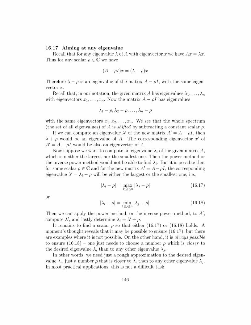
16.17 Aiming at any eigenvalueRecall that for any eigenvalue λ of A with eigenvector x we have Ax = λx.

Thus for any scalar ρ ∈ C we have

(A− ρI)x = (λ− ρ)x

Therefore λ− ρ is an eigenvalue of the matrix A− ρI, with the same eigen-vector x.

Recall that, in our notation, the given matrix A has eigenvalues λ1, . . . , λnwith eigenvectors x1, . . . , xn. Now the matrix A− ρI has eigenvalues

λ1 − ρ, λ2 − ρ, . . . , λn − ρ

with the same eigenvectors x1, x2, . . . , xn. We see that the whole spectrum(the set of all eigenvalues) of A is shifted by subtracting a constant scalar ρ.

If we can compute an eigenvalue λ′ of the new matrix A′ = A− ρI, thenλ + ρ would be an eigenvalue of A. The corresponding eigenvector x′ ofA′ = A− ρI would be also an eigenvector of A.

Now suppose we want to compute an eigenvalue λi of the given matrix A,which is neither the largest nor the smallest one. Then the power method orthe inverse power method would not be able to find λi. But it is possible thatfor some scalar ρ ∈ C and for the new matrix A′ = A−ρI, the correspondingeigenvalue λ′ = λi − ρ will be either the largest or the smallest one, i.e.,

|λi − ρ| = max1≤j≤n

|λj − ρ| (16.17)

or|λi − ρ| = min

1≤j≤n|λj − ρ|. (16.18)

Then we can apply the power method, or the inverse power method, to A′,compute λ′, and lastly determine λi = λ′ + ρ.

It remains to find a scalar ρ so that either (16.17) or (16.18) holds. Amoment’s thought reveals that it may be possible to ensure (16.17), but thereare examples where it is not possible. On the other hand, it is always possibleto ensure (16.18) – one just needs to choose a number ρ which is closer tothe desired eigenvalue λi than to any other eigenvalue λj.

In other words, we need just a rough approximation to the desired eigen-value λi, just a number ρ that is closer to λi than to any other eigenvalue λj.In most practical applications, this is not a difficult task.

146

16.18 Power method with shiftAssume that ρ is a rough approximation to an eigenvalue λi of A, i.e., ρ

is closer to λi than to any other eigenvalue λj of A:

|λi − ρ| < |λj − ρ| ∀j 6= i.

Then the matrix A′ = A − ρI will have the smallest eigenvalue λ′ = λi − ρwith the eigenvector x′ = xi.

We can apply the inverse power method to A′ = A−ρI. It will give us thesmallest eigenvalue λ′ and a corresponding eigenvector x′ of the matrix A′.Then we can determine λi = λ′ + ρ and xi = x′, i.e., the desired eigenvalueand eigenvector of A. This trick is called the power method with shift, becauseit is based on shifting the eigenvalues of A by a conveniently chosen scalarρ ∈ C. That scalar is called the shift.

According to Theorem 16.9 and (16.15), the power method with shift ρconverges linearly, with the ratio

r =|λi − ρ|

minj 6=i |λj − ρ|< 1. (16.19)

16.19 Note on the speed of convergenceThe speed of convergence of the power method depends on how big or

small the ratio r is; see Section 16.4. If r is small (close to zero), the con-vergence is actually pretty fast6. So it is in our best interests to select thescalar ρ so that r will be small. Fortunately, this is often possible.

The formula (16.19) suggests that if we keep changing ρ so that ρ→ λi,then the numerator and denominator of (16.19) have the following limits:

|λi − ρ| → 0minj 6=i |λj − ρ| → minj 6=i |λj − λi| > 0

}=⇒ r → 0.

Thus, the better ρ approximates λi, the smaller r is, and the faster theconvergence will be. We will explore this idea in the next section.

6For example, if r = 0.1, then each iteration adds one accurate decimal digit; hence,in single precision, 6–7 iterations might give us maximum accuracy. If r = 0.01, theneach iteration adds two accurate decimal digits, i.e., 6–7 iterations might suffice in doubleprecision.

147

16.20 Power method with Rayleigh quotient shiftAs it turns out, we do not have to work hard to provide a good approx-

imation ρ to λi that would accelerate the convergence – the power methoditself can do this for us.

Recall that at each iteration we find a vector qk that gets closer andcloser to the eigenspace span{xi} corresponding to the eigenvalue λi of the

matrix A. Thus the corresponding Rayleigh quotientq∗kAqkq∗kqk

would get closer

and closer to λi. Why not to use this Rayleigh quotient as the best availableapproximation to λi? In other words, at every iteration we can reset (update)the shift ρ by using the Rayleigh quotient of the vector qk obtained at theprevious iteration.

This suggests the following scheme. First, one chooses an initial vector q0

and an initial shift ρ0 (which does not have to be a very good approximationto λi). Then for each k ≥ 1 one computes

qk =(A− ρk−1I)−1qk−1

σk(16.20)

where σk is a convenient scaling factor, for example, σk = ‖(A−ρk−1I)−1qk−1‖,and one updates the shift by

ρk =q∗kAqkq∗kqk

This brilliant scheme is known as power method with Rayleigh quotient shift.Its convergence is, generally, quadratic (better than linear). If the matrix

A is Hermitian, the convergence is even faster – it is cubic!!!

16.21 ExampleConsider the symmetric matrix

A =

2 1 11 3 11 1 4

and let q0 = (1, 1, 1)T be the initial vector and q0 = 5 the initial shift. When powermethod with Rayleigh quotient shift is applied to A, the following values ρk are computedat the first two iterations:

ρ1 = 5.2131, ρ2 = 5.214319743184

The actual value is λ = 5.214319743377. After only two iterations, the method produces

10 accurate digits. The next iteration would bring about 30 accurate digits – more than

enough for double precision arithmetic.

148

16.22 Power method: pros and cons

(a) The power method is classic. Its logic is simple, and the method gen-erally works well. The convergence is quadratic, and for Hermitianmatrices the convergence is cubic.

(b) The power method is still very slow for two reasons. The main one isthat each iteration is rather expensive. Indeed, according to (16.20)we need to compute (A − ρk−1I)−1qk−1, i.e., solve a system of linearequations (A−ρk−1I)x = qk−1. This can be done by LU decompositionof the matrix A− ρk−1I, which keeps changing at every iteration (be-cause of ρk−1). Hence the LU decomposition must be performed anewat every iteration, and each LU decomposition takes ≈ 2n3/3 flops(Section 7.10). Thus the cost of computing one eigenvalue is ≈ 2pn3/3,where p is the number of iterations (typically, p is about 5 or 10).

The other reason is that each eigenvalue must be computed indepen-dently – we need to choose an initial vector q0 and an initial shift ρ0, andthen run the inverse power method until its iterations converge. Thus,if we want to compute all n eigenvalues of A, the total computationalcost will be 2pn4/3 flops. This is quite a big number.

(c) Lastly, if the matrix A is real (and this is the most common case inpractice), then in order to compute its non-real complex eigenvaluesλi /∈ R one has to use complex shifts ρk /∈ R. Thus one has to deal withcomplex matrices (A− ρk−1I), which is inconvenient and expensive.

It would be nice to operate with real matrices only, for as long aspossible, and obtain pairs of complex conjugate eigenvalues only at thevery last step. The QR algorithm, to be discussed in the next chapter,provides such a luxury.

Exercise 16.1. (JPE, May 2003) Let A be a symmetric matrix with eigenvalues such that|λ1| > |λ2| ≥ · · · ≥ |λn−1| > |λn|. Suppose z ∈ Rn with zTx1 6= 0, where Ax1 = λ1x1.Prove that, for some constant C,

limk→∞

Akz

λk1= Cx1

and use this result to devise a reliable algorithm for computing λ1 and x1. Explain howthe calculation should be modified to obtain (a) λn and (b) the eigenvalue closest to 2.

149

Exercise 16.2. (JPE, September 1996) The matrix

A =

2 0 00 1 20 2 1

has eigenpairs

(λ, x) =

2,

100

,

−1,

01−1

,

3,

011

,

Suppose the power method is applied with starting vector

z0 = [1, 1,−1]t/√

3

(a) Determine whether or not the iteration will converge to an eigenpair of A, and ifso, which one. Assume exact arithmetic.

(b) Repeat (a), except now use the inverse iteration with the same starting vector z0

and the Rayleigh quotient of z0 as approximation for the eigenvalue.

(c) Now answer both (a) and (b) again, except this time use standard fixed precisionfloating point arithmetic, i.e. computer arithmetic.

150

Chapter 17

Computation of Eigenvalues: QR Algorithm

In this last chapter of the course we present the QR algorithm for com-puting eigenvalues of any matrix A ∈ Cn×n. The QR algorithm (not to beconfused with QR decomposition!) dates back to the early 1960s, and inthe recent decades it became the most widely used method for calculatingeigenvalues.

17.1 “Pure” QR algorithmLet A ∈ Cn×n. The algorithm starts with A0 = A and generates a

sequence of matrices Ak defined as follows:

Ak−1 = QkRk (QR decomposition)

Ak = RkQk (reverse multiplication)

That is, a QR decomposition of the current matrix Ak−1 is computed first, and

then its factors are multiplied together in the reverse order to produce the next

matrix Ak. One iteration of the QR algorithm is called QR step. It consists of two

substeps: (i) QR decomposition and (ii) reverse multiplication.

17.2 Two basic facts

(i) All matrices Ak in the QR algorithm are unitary equivalent.

Proof. Indeed, Ak = RkQk = Q−1k Ak−1Qk. �

As a result, all matrices Ak have the same eigenvalues. They also have the same

2-condition number, ensuring that the QR algorithm is numerically stable.

(ii) If A is a Hermitian matrix, then all Ak’s are Hermitian matrices as well.

Proof. This follows from (i) and Section 3.10. �

The fact (b) ensures that the important Hermitian property is not lost during the

QR procedure.

151

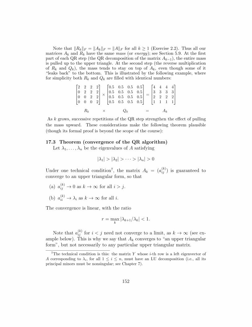
Note that ‖Rk‖F = ‖Ak‖F = ‖A‖F for all k ≥ 1 (Exercise 2.2). Thus all ourmatrices Ak and Rk have the same mass (or energy); see Section 5.9. At the firstpart of each QR step (the QR decomposition of the matrix Ak−1), the entire massis pulled up to the upper triangle. At the second step (the reverse multiplicationof Rk and Qk), the mass tends to stay on top of Ak, even though some of it“leaks back” to the bottom. This is illustrated by the following example, wherefor simplicity both Rk and Qk are filled with identical numbers:

2 2 2 20 2 2 20 0 2 20 0 0 2

×

0.5 0.5 0.5 0.50.5 0.5 0.5 0.50.5 0.5 0.5 0.50.5 0.5 0.5 0.5

=

4 4 4 43 3 3 32 2 2 21 1 1 1

Rk × Qk = Ak

As k grows, successive repetitions of the QR step strengthen the effect of pulling

the mass upward. These considerations make the following theorem plausible

(though its formal proof is beyond the scope of the course):

17.3 Theorem (convergence of the QR algorithm)Let λ1, . . . , λn be the eigenvalues of A satisfying

|λ1| > |λ2| > · · · > |λn| > 0

Under one technical condition7, the matrix Ak = (a(k)ij ) is guaranteed to

converge to an upper triangular form, so that

(a) a(k)ij → 0 as k →∞ for all i > j.

(b) a(k)ii → λi as k →∞ for all i.

The convergence is linear, with the ratio

r = maxk|λk+1/λk| < 1.

Note that a(k)ij for i < j need not converge to a limit, as k →∞ (see ex-

ample below). This is why we say that Ak converges to “an upper triangularform”, but not necessarily to any particular upper triangular matrix.

7The technical condition is this: the matrix Y whose i-th row is a left eigenvector ofA corresponding to λi, for all 1 ≤ i ≤ n, must have an LU decomposition (i.e., all itsprincipal minors must be nonsingular; see Chapter 7).

152

17.4 Example

Here we apply the QR algorithm to the matrix A =

[3 21 1

]. The cal-

culations were performed with MATLAB R©, and the QR decomposition wasdone by the standard MATLAB function qr.

Ak−1 Qk Rk Ak = RkQk

k = 1

[+3.0000 +2.0000+1.0000 +1.0000

] [−0.9487 −0.3162−0.3162 +0.9487

] [−3.1623 −2.2136

0 +0.3162

] [+3.7000 −1.1000−0.1000 +0.3000

]

k = 2

[+3.7000 −1.1000−0.1000 +0.3000

] [−0.9996 +0.0270+0.0270 +0.9996

] [−3.7014 +1.1077

0 +0.2702

] [+3.7299 +1.0073+0.0073 +0.2701

]

k = 3

[+3.7299 +1.0073+0.0073 +0.2701

] [−1.0000 −0.0020−0.0020 +1.0000

] [−3.7299 −1.0078

0 +0.2681

] [+3.7319 −1.0005−0.0005 +0.2681

]

k = 4

[+3.7319 −1.0005−0.0005 +0.2681

] [−1.0000 +0.0001+0.0001 +1.0000

] [−3.7319 +1.0006

0 +0.2680

] [+3.7320 +1.0000+0.0000 +0.2680

]

k = 5

[+3.7320 +1.0000+0.0000 +0.2680

] [−1.0000 −0.0000−0.0000 +1.0000

] [−3.7320 −1.0000

0 +0.2679

] [+3.7321 −1.0000−0.0000 +0.2679

]

The matrix Ak converges to an upper triangular form: its diagonal com-ponents converge to the eigenvalues of A:

λ1 = 2 +√

3 ≈ 3.7321, λ2 = 2−√

3 ≈ 0.2679,

its component below the diagonal converges to zero, and its component abovethe diagonal oscillates between two limit points: +1 and −1.

17.5 Advantages of the QR algorithm

(a) The QR algorithm produces all eigenvalues of A in “one go”, by a singlesequence of iterations. By contrast, the power method (Chapter 16)requires a separate sequence of iterations for each eigenvalue.

(b) The QR algorithm does not require an initialization – there is no needfor an arbitrary choice of an initial vector q0 or an initial shift ρ0 thatthe power method relies upon.

(c) An important case is that of a Hermitian matrix A. We know thatall the Ak’s are Hermitian matrices, too. Since the lower triangle ofAk converges to zero, so does its mirror image – the upper triangle.Therefore Ak converges to a diagonal matrix, a very nice result.

153

Despite all the obvious advantages, the “pure” QR algorithm is still quiteexpensive. Mainly, each iteration is very costly: the QR decomposition takes 2n3

flops (Sect. 9.8), and the multiplication of two n×n matrices Rk and Qk generallytakes 2n3 flops, as one can verify directly. We can take advantage of the triangularstructure of Rk and avoid multiplications by zeros, then the cost of multiplicationRk ×Qk will be half of 2n3 flops, i.e., n3 flops. This makes it 3n3 flops total, foreach QR step. Thus if we make p QR steps, the total cost will be 3pn3.

This seems to be an improvement over 2pn4/3 flops needed by the powermethod (Section 16.22), but in practice this cost is still too high. We also need toremember that the convergence is slow (linear), thus the pure QR algorithm mayrequire many more iterations than the power method does (see Section 16.3).

Fortunately, the computational cost can be dramatically reduced with the help

of Hessenberg matrices, see below. The use of Hessenberg matrices will also allow

us to develop tricks that speed up the convergence, from linear to quadratic.

17.6 Hessenberg matrixA ∈ Cn×n is called an (upper) Hessenberg matrix if aij = 0 for all i > j+1,

i.e., whenever A has the form

A =

× × · · · · · · ×

× ×. . .

. . ....

0 × ×. . .

......

. . .. . .

. . ....

0 · · · 0 × ×

Thus, A may have non-zero components in its upper triangle and on its

subdiagonal. It is just “one step away” from being an upper triangular.Recall that an upper triangular matrix has its eigenvalues on its diagonal,

i.e., its eigenvalues are “exposed”. The eigenvalues of a Hessenberg matrix are

not exposed, they are “hidden”, but if any subdiagonal component is zero, i.e.,

ai+1,i = 0 for some i, then the eigenvalue problem can be simplified:

17.7 Lucky reduction of the eigenvalue problemSuppose A is Hessenberg and ai+1,i = 0 for some 1 ≤ i ≤ n− 1. Then A has a

block-diagonal structure

A =

[A1 B0 A2

]where A1 ∈ Ci×i and A2 ∈ C(n−i)×(n−i). Now the eigenvalues of A consist of those

of A1 and A2. Thus it is enough to find the eigenvalues of the two smaller matrices

A1 and A2, while the matrix B can be completely ignored.

154

17.8 Theorem (Hessenberg decomposition)Every matrix A ∈ Cn×n is unitary equivalent to a Hessenberg matrix, i.e.

A = Q∗HQ

where H is a Hessenberg matrix and Q is a unitary matrix. There is an exactfinite algorithm (Arnoldi algorithm) for computing H and Q.

Proof. The matrix equation A = Q∗HQ can be rewritten as AQ∗ = Q∗H. Denote byqi, 1 ≤ i ≤ n, the columns of the unitary matrix Q∗ and by hij the entries of H. Equatingthe columns of the matrices AQ∗ and Q∗H (and remembering that hij = 0 for i > j + 1)we obtain the following system of equations

Aq1 = h11q1 + h21q2

Aq2 = h12q1 + h22q2 + h32q3

· · ·Aqi = h1iq1 + · · ·+ hiiqi + hi+1,iqi+1

· · ·Aqn = h1nq1 + · · ·+ hn−1,nqn−1 + hn,nqn

Note that the last equation is slightly different from the others, since it terminates on adiagonal entry of H.

Now the Arnoldi algorithm goes along the lines similar to the classical Gram-Schmidtorthogonalization. We pick an arbitrary unit vector q1, compute v1 = Aq1 and

w2 = v1 − 〈v1, q1〉 q1

It is easy to check that w2 will be orthogonal to q1. Then we set h11 = 〈v1, q1〉 andh21 = ‖w2‖ and define q2 = w2/‖w2‖. This enforces the first equation in the abovesystem.

Then, for every i = 2, . . . , n− 1 we make four steps:

Step 1: compute vi = Aqi.

Step 2: for all j = 1, . . . , i compute hji = 〈vi, qj〉.Step 3: compute wi = vi −

∑ij=1 hjiqj .

(note: the vector wi is guaranteed to be orthogonal to q1, . . . , qi).

Step 4: compute hi+1,i = ‖wi‖ and qi+1 = wi/hi+1,i.

Finally, for i = n we execute steps 1 and 2 only.

An exception may occur at step 4 if it happens that hi+1,i = 0. In that case we simply

pick an arbitrary unit vector qi+1 orthogonal to q1, . . . , qi and continue the procedure “as

if nothing happened”. �

155

The exceptional case hi+1,i = 0 in Step 4 is sometimes referred to as thebreakdown of the Arnoldi algorithm. This term is quite misleading, however, sincethe method does not really break down. In fact, the resulting Hessenberg matrixH will then have a simpler structure leading to a lucky reduction of the eigenvalueproblem (Secion 17.7).

The matrices H and Q in Theorem 17.8 are far from being unique. The very

first step of the Arnoldi algorithm is based on an arbitrary choice of a unit vector

q1 (the first column of Q∗). Actually, by choosing a simple vector q1 (such as

q1 = e1), we can reduce the amount of computational work, see next.

17.9 Cost of Arnoldi algorithmThe cost of Step 1 is 2n2 flops, the cost of Step 2 is 2ni flops, the same for

Step 3, and lastly Step 4 takes 3n flops. The total cost is then

n∑i=1

(2n2 + 4ni+ 3n) ∼ 4n3

(by choosing q1 = e1 one can save some work and compute H and Q in 103 n

3 flops;see the textbook for more details). This cost is comparable to the cost of one QRstep for a generic (non-Hessenberg) matrix.

The Hessenberg decomposition can be regarded as a pre-processing of the ma-

trix A; it only needs to be done once, and then the QR algorithm can be applied to

the resulting Hessenberg matrix. It is important, obviously, that the Hessenberg

property is not lost during the QR iterations.

17.10 Preservation of Hessenberg structureIf an invertible matrix A0 is Hessenberg, then all the matrices Ak gener-

ated by the QR algorithm will be Hessenberg matrices as well.

Proof. By induction, let Ak−1 be Hessenberg. Then Ak−1 = QkRk and so Qk =

Ak−1R−1k . This is a product of a Hessenberg matrix Ak−1 and an upper triangular matrix

R−1k . One can verify by direct inspection that such a product is always a Hessenberg

matrix. Now Ak = RkQk is also a product of an upper triangular matrix Rk and a

Hessenberg matrix Qk, so it is a Hessenberg matrix, too. �

For a noninvertible Hessenberg matrix A0, the above property remains valid,

but the proof is more complicated and we leave it out. Basically, one can show

that Qk constructed by Gram-Schmidt orthogonalization (Chapter 9) is also Hes-

senberg, thus Ak will again be a Hessenberg matrix.

156

17.11 Cost of a QR step for Hessenberg matricesFor Hessenberg matrices, the QR algorithm can be implemented with a sub-

stantial reduction of computational cost. First, the QR decomposition can be done

via Givens rotators, it will take 6n2 flops, according to Section 14.15. Second, Qkis a product of n−1 rotators, and the multiplication of Rk by Qk can be organized

so that it will take ≤ 6n2 flops (we omit details). The total for one QR step is

then ≤ 12n2 flops, a dramatic drop from 3n3 flops required for a non-Hessenberg

matrix A (as we said after Section 17.5).

“Pure” QR:

QR withHessenberg:

A

A0

A0

A1

A1103 n

312n2

3n3

A2

A2

12n2

3n3

A3

A3

12n2

3n3

A4

A4

12n2

3n3

A5

A5

12n2

3n3

17.12 The case of Hermitian matricesAn important case is that of Hermitian matrices. In that case A0 will be

both Hermitian (Section SAequiv) and Hessenberg. Hence A0 will be a tridiagonalmatrix (hij = 0 for all |i− j| > 1). Its construction by the Arnoldi algorithm takesonly 4

3n3 flops (see the textbook for details).

The use of Hessenberg matrices greatly reduces the cost of each QR step.Another standing issue is a slow (linear) convergence (Theorem 17.3), with ratio

r = maxk|λk+1/λk| < 1. (17.1)

For example, if A has eigenvalues 1, 9, and 10, then the ratio is r = 0.9, and the

process would be crawling. Fortunately, we have improvement in this respect, too:

17.13 Theorem (without proof)Assume that A0, and hence Ak for all k ≥ 1, are Hessenberg matrices.

Then the convergence a(k)i,i−1 → 0 as k → ∞ in Theorem 17.3 is linear with

ratio ri = |λi/λi−1|. In addition, the convergence a(k)nn → λn is linear with

ratio rn = |λn/λn−1|.Now each subdiagonal entry a

(k)i,i−1 has its own ratio of convergence ri, so some

may converge faster than others. The convergence is no longer governed by one

single ratio (17.1). For example, if A has eigenvalues 1, 9, and 10, then the last

(bottom) subdiagonal entry converges with ratio r = 1/9, which is very fast. This

new flexibility allows us to develop smart tricks accelerating the convergence of

some selected entries first, and then all the remaining entries.

157

17.14 QR algorithm with shiftOne can modify the matrix A to decrease the ratio rn = |λn/λn−1| and

thus make the convergence

a(k)n,n−1 → 0 and a(k)

nn → λn

of the two bottom entries faster.This can be done with the help of shifting, as in Section 16.18. Recall that

for any ρ ∈ C the matrix A− ρI has eigenvalues λ1− ρ, . . . , λn− ρ. The newmatrix A − ρI is still Hessenberg (or Hermitian) if A itself was Hessenberg(resp., Hermitian), so we lose nothing by replacing A with A− ρI.

Now suppose ρ is a good approximation to the smallest eigenvalue λn. Ifwe apply the QR steps to the matrix A′ = A − ρI, then the convergence ofthe two bottom entries of the new matrix will be linear with ratio

r′n = |λn − ρ|/|λn−1 − ρ|.

Now we can control the speed of convergence by choosing/adjusting the shiftρ. Obviously, if ρ → λn, then r′n → 0. Thus the better ρ approximates λnthe faster the convergence of the two bottom entries will be.

17.15 QR algorithm with Rayleigh quotient shiftThe approximation ρ can be updated at every iteration, as in Section 16.20,

by using the Rayleigh quotient

ρ = ρk = u∗kAkuk

where uk is an approximate unit eigenvector of the matrix Ak correspondingto its smallest eigenvalue λn. In practice, a simple and convenient choice foruk is uk = en, which gives ρk = a

(k)nn . Then the QR algorithm with shift goes

as follows:

Ak−1 − ρk−1I = QkRk (QR decomposition of Ak−1 − ρk−1I)

RkQk + ρk−1I = Ak (computation of the next matrix Ak)

ρk = a(k)nn (setting ρk to the trailing entry of Ak)

This is called the Rayleigh quotient shift. The convergence of the two bottomentries of Ak is now quadratic, basically for the same reasons as it was inSection 16.20.

158

The use of Rayleigh quotient shift allows us very quickly – say, in about five

iterations – to “kill” the bottom subdiagonal entry a(k)n,n−1 and find the smallest

eigenvalue λn of the matrix A. But the other subdiagonal entries, a(k)i+1,i, 1 ≤ i ≤

n − 2, will move to zero slowly – linearly, with variable ratios. For example if Ahas eigenvalues 1, 9, and 10, then the smallest one will be found very fast, butthe other two may take 50–100 (or more) iterations, because the convergence willproceed with a pretty bad ratio r = 0.9.

So we apply one more trick – the “lucky reduction” described in Section 17.7

– to “split off” the smallest eigenvalue λn and reduce the size of the matrix A:

17.16 QR algorithm with deflationWhen a

(k)n,n−1 becomes practically zero and a

(k)nn becomes practically equal

to λn, the matrix Ak will have the following form:

Ak =

[Ak bk0 λn

]where Ak is an (n−1)× (n−1) Hessenberg matrix. Its eigenvalues are thoseof A, minus λn, i.e., they are λ1, . . . , λn−1. Now we can apply further steps ofthe QR algorithm (with shift) to the matrix Ak, instead of Ak. This quicklyproduces its smallest eigenvalue, λn−1, which can be split off in the samemanner. Then we reduce our matrix further, to the size (n − 2) × (n − 2),and so on. This procedure is called the deflation of the matrix A:

“cutting lines” are in red

In practice, each eigenvalue of A requires just 3-5 iterations (QR steps),on the average. For Hermitian matrices, it is even faster – just 2-3 iterationsper eigenvalue. Remember also that each QR step for Hessenberg matrices isvery cheap (just 12n2 flops). This is how the QR algorithm with Hessenbergmatrices, Rayleigh quotient shift, and deflation achieves a top speed.

The above procedure works well on generic matrices, but it fails occasionally

in certain exceptional cases. One such case is a matrix A with two equally large

eigenvalues, i.e., |λi| = |λj | for some i 6= j. Such a matrix does not meet the

requirements of Theorem 17.3, so the convergence is not guaranteed. In that case

the QR algorithm may “get stuck”, as illustrated by the following example.

159

17.17 Example

Let A =

[0 11 0

]. Note that A is already a Hessenberg matrix, thus the Hessenberg

decomposition is not needed here. Now the pure QR algorithm gives

A0 = Q1R1 =

[0 11 0

] [1 00 1

]hence

A1 = R1Q1 =

[1 00 1

] [0 11 0

]= A

and we are “back to square one”. The process goes nowhere. The Rayleigh quotient shift

ρ = a22 proposed in Section 17.15 has no effect either, since a22 = 0. The reason of this

failure is that the eigenvalues of A, which are +1 and −1, have equal absolute values –

this is a symmetry which confuses the QR algorithm, it “cannot decide” which eigenvalue

to approach. To break this symmetry, one needs to choose the shift ρ differently.

An alternative shift ρ can be used whenever the procedure “gets stuck”:

17.18 Wilkinson shiftAt step k of the QR algorithm with shift, let Bk denote the trailing 2×2 block

at the bottom right corner of Ak:

Bk =

[a

(k)n−1,n−1 a

(k)n−1,n

a(k)n,n−1 a

(k)n,n

](17.2)

Now set ρk to the eigenvalue of Bk that is closer to a(k)n,n (in case of a tie, either

one can be taken). This is called Wilkinson shift.

The eigenvalues of a 2 × 2 matrix can be easily (and precisely) computed by

the quadratic formula, whether they are real or complex. If they are real, then the

Wilkinson shift will help break the symmetry like in Example 17.17.

17.19 Example 17.17 continuedThe Wilkinson shift here is either ρ = 1 or ρ = −1. Let us choose ρ = −1. Then

A0 − ρI =

[1 11 1

]= Q1R1 =

[1/√

2 1/√

2

1/√

2 −1/√

2

] [√2√

20 0

]and then

A1 = R1Q1 + ρI =

[2 00 0

]+

[−1 0

0 −1

]=

[1 00 −1

].

The matrix A1 is diagonal and its diagonal entries are the eigenvalues of A.

So the QR algorithm with the Wilkinson shift converges in just one step.

160

Lastly, we discuss an important case of real matrices with complex eigenvalues.It was already mentioned in Section 16.22(c).

If the matrix A is real (which is the most common case in practice), then itscomplex eigenvalues come in conjugate pairs a±ib. They have equal absolute values|a+ bi| = |a− bi|, immediately violating the main assumption of Theorem 17.3.

Furthermore, the pure QR algorithm is bound to fail for the following simplereason. If A is real, then all Qk, Rk and Ak will be real matrices as well, thuswe cannot even expect the real diagonal entries of Ak to converge to the complexeigenvalues of A. In this case Ak may not converge to anything at all.

The QR algorithm with shift may be able to find complex eigenvalues of a

real matrix A, but it needs to use complex shifts ρ /∈ R and complex matrices

A − ρI, which is inconvenient and expensive. Fortunately, the QR algorithm can

be organized so that it operates with real matrices only, for as long as possible,

and obtains pairs of complex conjugate eigenvalues only at the very last step:

17.20 Wilkinson shifts for complex eigenvalues of real matricesSuppose at the step k of the QR algorithm, the matrix Ak is still real, but

the eigenvalues of its 2 × 2 trailing block Bk in (17.2) are non-real complexnumbers. Let us denote them by ρk and ρk (remember that they are complexconjugate to each other). Then the Wilkinson shift ρk will be a complexnumber, and the matrix Ak − ρkI will be complex, too. The QR step willthen produce a complex matrix Ak+1, which we do not really want.

In this case one can use the following trick to avoid further working withcomplex matrices: at the very next QR step we set ρk+1 = ρk, i.e., we choosethe shift ρk+1 to be the other complex eigenvalue of Bk. Then, remarkably,the resulting matrix Ak+2 will be real again, for the reasons explained bellow.

Furthermore, the values ρk and ρk will approximate two complex eigen-values of the matrix A. Therefore, the QR algorithm with Wilkinson shift isable to compute conjugate pairs of complex eigenvalues of a real matrix A,and stay with real matrices for as long as possible.

Actually, there is no need to compute the complex matrix Ak+1 mentionedabove. One can just combine the two QR steps together and construct Ak+2

directly from Ak (bypassing Ak+1). This can be carried out entirely in realarithmetic. The resulting all-real procedure is called the double-step QRalgorithm with Wilkinson shift.

In the following, all complex scalars and matrices are marked red. This includes matrix

A2, which will remain hypothetically complex until we prove that it is real.

161

17.21 Analysis of the double-stepLet A0 ∈ Rn×n be a real matrix. Let ρ and ρ be two complex non-real

conjugate numbers that are not eigenvalues of A0. Let us apply two QRsteps with the shifts ρ and ρ:

A0 − ρI = Q1R1 R1Q1 + ρI = A1 (17.3)

A1 − ρI = Q2R2 R2Q2 + ρI = A2 (17.4)

Since the matrices A0 − ρI and A1 − ρI are nonsingular, the above QRdecompositions may be constructed so that R1 and R2 have positive realentries, cf. Section 9.7. Then, remarkably, A2 will be a real matrix.

Proof. It follows from (17.3) that R1 = Q−11 A0 − ρQ−1

1 , hence

A1 = (Q−11 A0 − ρQ−1

1 )Q1 + ρI = Q−11 A0Q1

Similarly, it follows from (17.4) that R2 = Q−12 A1 − ρ Q−1

2 , hence

A2 = (Q−12 A1 − ρ Q−1

2 )Q2 + ρI = Q−12 A1Q2

Next we will compute the product (A0 − ρI)(A0 − ρI) in two ways. First,

(A0 − ρI)(A0 − ρI) = A20 − (ρ+ ρ)A0 + ρρI

= A20 − 2(Re ρ)A0 + |ρ|2I.

Since (Re ρ) and |ρ| are real numbers, the matrix A = (A0 − ρI)(A0 − ρI) is entirely real.On the other hand, we have

A = (A0 − ρI)(A0 − ρI)

= (A0 − ρI)Q1R1

= Q1Q−11 (A0 − ρI)Q1R1

= Q1(Q−11 A0Q1 − ρI)R1

= Q1(A1 − ρI)R1

= Q1Q2R2R1.

This is actually a QR decomposition of the matrix A, with orthogonal matrix Q = Q1Q2

and upper triangular matrix R = R2R1. Since the matrices R1 and R2 have positivediagonal entries, so does its product R. Therefore, according to Section 9.7, the above QRdecomposition is unique.

But every real matrix A has a real QR decomposition A = QR with positive diagonalentries of R (by Sections 9.5 and 9.6), hence by its uniqueness both matrices Q = Q1Q2

and R = R2R1 must be real. Lastly,

A2 = Q−12 A1Q2 = (Q1Q2)−1A0(Q1Q2) = Q−1A0Q.

As a product of three real matrices, A2 must be a real matrix as well. �

162

Exercise 17.1. (JPE, September 2009) Let A ∈ Cn×n be nonsingular. Let A = Q1R1

be a QR decomposition of A, and for k ≥ 1 define inductively AQk = Qk+1Rk+1, a QRdecomposition of AQk.

(a) Prove that there exists an upper triangular matrix Uk such that Qk = AkUk and alower triangular matrix Lk such that Qk = (A∗)−kLk.

(b) Suppose limk→∞Rk = R∞ and limk→∞Qk = Q∞ exist. Determine the eigenvaluesof A in terms of R∞.

Exercise 17.2. (JPE, May 2006) Let A ∈ Cn×n be tri-diagonal and Hermitian, with allits super-diagonal entries nonzero. Prove that the eigenvalues of A are distinct.

(Hint: show that for any scalar λ, the matrix A− λI has rank at least n− 1.)

163