Numerical investigation of the use of externally generated ... · Numerical investigation of the...
123
Numerical investigation of the use of externally generated Lorentz forces to improve the flow pattern in a continuous glass-melting tank Dissertation zur Erlangung des akademischen Grades Doktoringenieur (Dr.-Ing.) vorgelegt der Fakultät für Elektrotechnik und Informationstechnik der Technischen Universität Ilmenau von Herrn M.Sc. Senan Soubeih geboren am 01.06.1981 in Latakia, Syrien Gutachter: Priv.-Doz. Dr.-Ing. habil. Ulrich Lüdtke apl. Prof. Dr.-Ing. habil. Christian Karcher Univ.-Prof. Dr.-Ing. Egbert Baake Tag der wissenschaftlichen Aussprache: 20.10.2016 urn:nbn:de:gbv:ilm1-2016000518
Transcript of Numerical investigation of the use of externally generated ... · Numerical investigation of the...
Numerical investigation of the use of externally generated Lorentz forces to
improve the flow pattern in a continuous glass-melting tank
Dissertation
zur Erlangung des akademischen Grades
Doktoringenieur (Dr.-Ing.)
vorgelegt der
Fakultät für Elektrotechnik und Informationstechnik der
Technischen Universität Ilmenau
von Herrn
M.Sc. Senan Soubeih
geboren am 01.06.1981 in Latakia, Syrien
Gutachter:
Priv.-Doz. Dr.-Ing. habil. Ulrich Lüdtke
apl. Prof. Dr.-Ing. habil. Christian Karcher
Univ.-Prof. Dr.-Ing. Egbert Baake
Tag der wissenschaftlichen Aussprache: 20.10.2016
urn:nbn:de:gbv:ilm1-2016000518
Dissertation Senan Soubeih ii
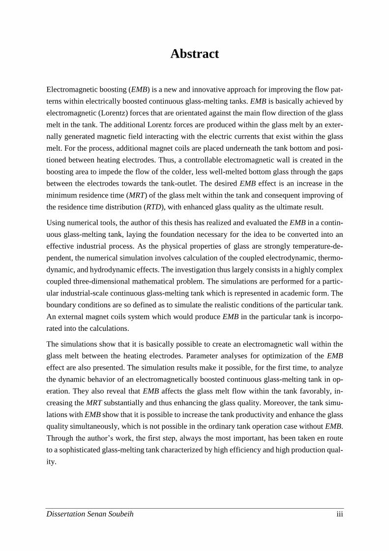
Zusammenfassung
Das elektromagnetische Boosting (EMB) ist ein neuer und innovativer Lösungsansatz zur Ver-
besserung der Strömungsverhältnisse in den kontinuierlich arbeitenden Glasschmelzwannen
mit einer elektrischen Zusatzbeheizung. Das EMB basiert auf der Benutzung von extern indu-
zierten Lorentzkräften, die entgegen der Hauptströmungsrichtung in der Schmelzwanne gerich-
tet sind. Die Generierung dieser zusätzlichen Lorentzkräfte erfolgt durch die Überlagerung ei-
nes externen Magnetfeldes mit der in der Glasschmelze fließenden elektrischen Ströme. Das
externe Magnetfeld wird von zusätzlichen Magnetspulen generiert. Diese werden unterhalb des
Wannenbodens zwischen den Elektroden der Zusatzbeheizung installiert. Dadurch wird ein
steuerbarer elektromagnetischer Wall in der Glasschmelze zwischen den Elektroden realisiert.
Dieser verhindert die unerwünschte Strömung der kälteren, bodennahen Glasschmelze zum
Wannenauslass. Als Ergebnis wird die minimale Verweilzeit (MRT) der Glasschmelze in der
Wanne erhöht und somit die Verweilzeitverteilung (RTD) verbessert. Als Ergebnis wird die
Glasqualität erhöht.
In dieser Dissertation wird das EMB in einer Glasschmelzwanne numerisch untersucht und so-
mit die Grundlage für eine industrielle Anwendung gelegt. Die stark temperaturabhängigen
Materialeigenschaften von Glas erfordern gekoppelte Berechnungen von Elektro-, Thermo-
und Hydrodynamik, die zu hochkomplexen, dreidimensionalen, numerischen Simulationen der
Problemstellung führen. Die Simulationen werden für eine reale industrielle Glasschmelz-
wanne unter Annahme einiger Vereinfachungen durchgeführt. Die Randbedingungen sind so
definiert, dass die realen Betriebsverhältnisse der Wanne simuliert werden können. Für das
EMB wird ein zusätzliches Spulensystem angepasst.
Die Simulationen zeigen, dass es im Prinzip möglich ist, einen steuerbaren elektromagnetischen
Wall im Boostingbereich zu erzeugen. Um die optimale Wirkung des EMB zu erzielen, sind
Parameterstudien durchgeführt worden. Mit diesen Simulationen wird erstmals das dynamische
Betriebsverhalten einer Glasschmelzwanne mit EMB untersucht. Die Ergebnisse zeigen, dass
die gewünschte wesentliche Erhöhung von MRT und die damit verbundene Verbesserung von
RTD mit Hilfe des EMB erzielbar sind, wodurch die Qualität des Endproduktes erhöht wird.
Des Weiteren kann mit Hilfe des EMB die Glasqualität verbessert und gleichzeitig der Durch-
satz der Wanne erhöht werden. Unter normalen Betriebsverhältnissen ohne das EMB ist dies
nicht möglich. Diese theoretischen Untersuchungen bilden den ersten Schritt, das EMB in der
Praxis zu testen und einzusetzen, um neuartige Glasschmelzwannen mit höherem Wirkungs-
grad und verbesserter Qualität des Glasproduktes in der Industrie einzuführen.
Dissertation Senan Soubeih iii
Abstract
Electromagnetic boosting (EMB) is a new and innovative approach for improving the flow pat-
terns within electrically boosted continuous glass-melting tanks. EMB is basically achieved by
electromagnetic (Lorentz) forces that are orientated against the main flow direction of the glass
melt in the tank. The additional Lorentz forces are produced within the glass melt by an exter-
nally generated magnetic field interacting with the electric currents that exist within the glass
melt. For the process, additional magnet coils are placed underneath the tank bottom and posi-
tioned between heating electrodes. Thus, a controllable electromagnetic wall is created in the
boosting area to impede the flow of the colder, less well-melted bottom glass through the gaps
between the electrodes towards the tank-outlet. The desired EMB effect is an increase in the
minimum residence time (MRT) of the glass melt within the tank and consequent improving of
the residence time distribution (RTD), with enhanced glass quality as the ultimate result.
Using numerical tools, the author of this thesis has realized and evaluated the EMB in a contin-
uous glass-melting tank, laying the foundation necessary for the idea to be converted into an
effective industrial process. As the physical properties of glass are strongly temperature-de-
pendent, the numerical simulation involves calculation of the coupled electrodynamic, thermo-
dynamic, and hydrodynamic effects. The investigation thus largely consists in a highly complex
coupled three-dimensional mathematical problem. The simulations are performed for a partic-
ular industrial-scale continuous glass-melting tank which is represented in academic form. The
boundary conditions are so defined as to simulate the realistic conditions of the particular tank.
An external magnet coils system which would produce EMB in the particular tank is incorpo-
rated into the calculations.
The simulations show that it is basically possible to create an electromagnetic wall within the
glass melt between the heating electrodes. Parameter analyses for optimization of the EMB
effect are also presented. The simulation results make it possible, for the first time, to analyze
the dynamic behavior of an electromagnetically boosted continuous glass-melting tank in op-
eration. They also reveal that EMB affects the glass melt flow within the tank favorably, in-
creasing the MRT substantially and thus enhancing the glass quality. Moreover, the tank simu-
lations with EMB show that it is possible to increase the tank productivity and enhance the glass
quality simultaneously, which is not possible in the ordinary tank operation case without EMB.
Through the author’s work, the first step, always the most important, has been taken en route
to a sophisticated glass-melting tank characterized by high efficiency and high production qual-
ity.
Contents
Dissertation Senan Soubeih iv
Contents
1 Introduction ....................................................................................................................... 1
1.1 Glass processing .......................................................................................................... 1
1.2 Numerical simulation in glass technology ................................................................... 2
1.3 About this work ........................................................................................................... 3
2 Continuous glass-manufacturing process ....................................................................... 4
2.1 Continuous glass-melting systems............................................................................... 4
2.2 Flow patterns within continuous glass-melting tanks.................................................. 6
2.3 Residence time distribution (RTD) .............................................................................. 7
3 Electric boosting (EB) ....................................................................................................... 9
3.1 Flow control in continuous glass-melting tanks .......................................................... 9
3.2 Continuous glass-melting tanks with barrier booster ................................................ 10
4 Scope of thesis .................................................................................................................. 13
4.1 Concept of electromagnetic boosting (EMB) ............................................................ 13
4.2 Aim and objectives of the thesis ................................................................................ 15
4.3 Overview of the thesis ............................................................................................... 17
5 Literature, state of the art .............................................................................................. 19
5.1 Numerical simulation of glass-melting tanks ............................................................ 19
5.2 Lorentz forces in glass manufacture .......................................................................... 21
5.2.1 Natural Lorentz forces ........................................................................................ 21
5.2.2 Artificial Lorentz forces ..................................................................................... 23
6 Problem formulation ...................................................................................................... 27
6.1 Tank representation ................................................................................................... 27
6.2 Mathematical model .................................................................................................. 30
6.2.1 Glass material properties .................................................................................... 30
6.2.2 Electromagnetic field ......................................................................................... 31
6.2.3 Flow and temperature fields ............................................................................... 33
7 Numerical methodology .................................................................................................. 35
7.1 Coupling the calculations .......................................................................................... 35
Contents
Dissertation Senan Soubeih v
7.2 Calculating electromagnetic field with FLUENT ..................................................... 36
7.3 Validation by numerical simulation with MAXWELL ............................................. 38
7.3.1 Boundary conditions of the cube-model ............................................................ 39
7.3.2 Results of comparison ........................................................................................ 40
7.4 A simplified tank model with two electrodes ............................................................ 49
7.4.1 The model employed .......................................................................................... 50
7.4.2 Boundary conditions of the middle-section model ............................................ 51
7.4.3 Computational grid and numerical solution ....................................................... 52
7.4.4 Results from the middle-section model .............................................................. 52
7.5 Calculating a steady-state AC system with FLUENT ............................................... 58
8 Numerical grid, solution, and accuracy ........................................................................ 61
8.1 Computational grid .................................................................................................... 61
8.2 Numerical solution .................................................................................................... 63
8.3 Verification and accuracy .......................................................................................... 64
8.3.1 Mesh-convergence study .................................................................................... 65
8.3.2 Residual evaluation study ................................................................................... 67
9 Implementation and results ........................................................................................... 69
9.1 The baseline-case ....................................................................................................... 69
9.1.1 Boundary conditions .......................................................................................... 69
9.1.2 Selected results of the baseline-case simulation ................................................ 72
9.2 Adapting the EMB system ......................................................................................... 76
9.3 Optimizing the EMB system ...................................................................................... 78
9.3.1 The optimum MRT ............................................................................................. 78
9.3.2 Coil diameter study ............................................................................................ 79
9.4 Comparison between the baseline-case and EMB-case ............................................ 81
9.5 Increasing the tank productivity ................................................................................ 87
9.6 Increasing the tank thermal efficiency ....................................................................... 90
9.7 Considering the structural steel girders ..................................................................... 93
9.7.1 Boundary conditions .......................................................................................... 94
Contents
Dissertation Senan Soubeih vi
9.7.2 Results and discussion ........................................................................................ 95
10 Conclusion and outlook .................................................................................................. 99
10.1 Conclusion ............................................................................................................. 99
10.2 Outlook ................................................................................................................ 100
Bibliography ......................................................................................................................... 101
List of abbreviations ............................................................................................................. 110
List of symbols ...................................................................................................................... 111
Chapter 1: Introduction
Dissertation Senan Soubeih 1
1 Introduction
Glass is a unique material that has been manufactured and used without interruption for more
than 5000 years. Glass-making is a very ancient form of industry that is still evolving and con-
stantly improving as the uses for glass expand. A full insight into the evolution of glass making
technology including its cultural implications over the millennia is presented in [1–4].
1.1 Glass processing
Today, life is unthinkable without glass, the manifold uses of which extend into almost every
field of modern science, industry, and our personal lives. Examples are containers, architecture,
touch screens, electronics, communication equipment, medical equipment, laboratory equip-
ment, optics, automotive, aircraft, or spaceship. Glass has been vital to technological advance-
ment, being continually proposed for new applications. Detailed descriptions of glass types and
their applications are given in [4–7].
The most important commercial glasses today are container glass (mainly for holding foods and
drinks) and flat glass (mainly for architecture and automotive applications). These glasses be-
long to a glass type called “soda-lime glass”, and are basically composed of soda (Na2O) and
lime (CaO) beside the main component, namely silica sand (SiO2).
The raw materials that are used for commercial glass manufacture are some of the most abun-
dant in the Earth’s crust, see [8,9] for comprehensive information. After suitable treatment,
these raw materials are weighed and mixed together to the desired composition forming what
is called “batch”. The process in which the raw materials are stored, weighed, mixed, and de-
livered to the melting furnaces is called “batching”. In modern manufacture, it has been fully
automated and improved by computer systems, e.g. [10,11]. Crushed glass called “cullet”,
which helps to accelerate the melting of the sand and to reduce the energy required for melting,
is also added to the batch. Nowadays, recycling of waste glass is becoming increasingly im-
portant to reduce the consumption of energy as well as raw materials.
After the batching stage, a glass-melting furnace receives the batch and heats it strongly to start
the melting, which is the major stage in the glass manufacturing process. Since commercial
glasses are needed in huge amounts, the batch is fed non-stop into the furnace and glass is
melted in a continuous manner. At the end of the melting stage, the glass melt, which has been
obtained, is delivered to forming devices, or molds, for the forming stage, in which glass melt
will cool to the desired shape.
Chapter 1: Introduction
Dissertation Senan Soubeih 2
Glass-melting furnaces are mostly tank-furnaces heated by fossil fuels (natural gas or fuel oils)
and electric power, sometimes independently and sometimes in combination. These tank-fur-
naces are operated continuously for high-tonnage production with a steady flow of glass melt
into the automatic forming devices. The successive processes of glass manufacturing including
the various types of construction and device are thoroughly covered in [12–14].
The flow of molten glass within the glass-melting tank is mainly driven by natural convection
of mass. The flow pattern itself plays an important role in the achievement of a qualitatively
acceptable glass product. Hence, controlling the flow patterns within the glass-melting tanks so
as to improve tank performance is one of the glass industry’s primary challenges. However,
controlling the glass melt flow in these tanks is fraught with difficulties.
1.2 Numerical simulation in glass technology
When industrial processes are being analysed, numerical simulation is an effective tool. It can
predict the dynamic regime behavior after changes in process conditions. Moreover, if systems
are to be developed that involve risky working conditions and high constructional costs, as the
case with continuous glass-melting tanks, numerical simulation offers wide possibilities at low
cost and with rapid response time and no risk involved. Thus, numerical models have come to
be of vital importance in the development of industrial systems.
In the glass industry, numerical simulation is now a reliable and effective tool for developing
new products, reducing production costs, and improving glass quality. It also offers the possi-
bility in glass manufacture of obtaining data that are difficult to measure in the real process and
of finding new parameter configurations without disturbing the operation.
Sine qua non to the simulation of industrial operations which involve highly complicated chem-
ical and physical processes, such as glass melting process, is a deep understanding of the un-
derlying physics and chemistry. As yet, there is no simulation tool that covers all processes in
glass technology. Computational fluid dynamics (CFD) is often the basis of the mathematical
models. The CFD models are linked with additional sub-models that have been developed to
simulate different problems in the glass melting process. Several special purpose software pack-
ages are thus used and linked together.
The glass industry is always in search of ways of optimizing the glass manufacturing process
especially improving glass quality and reducing energy consumption. Numerical models of
glass technology are essential not only for optimizing current furnace design and operating pa-
rameters, but also for studying new furnace designs and evaluating new techniques. Thus, nu-
merical models provide a solid foundation for important development decisions.
Chapter 1: Introduction
Dissertation Senan Soubeih 3
1.3 About this work
This thesis extends the possibilities for the development of industrial glass-melting tanks. The
author shows his numerical investigation of the potential of an unconventional method for con-
trolling the flow pattern within a continuous glass-melting tank. The method relies on electro-
magnetic flow control, where additionally generated electromagnetic (Lorentz) forces are
brought to bear on the glass melt. To do so, an additional magnet system must be adapted and
installed. This new and innovative approach is called “electromagnetic boosting”. The approach
of employing additionally generated Lorentz forces to improve the flow patterns in continuous
glass-melting tanks is, as yet, by no means an established technique. This thesis with its numer-
ical investigation represents the sole groundwork to date for an industrial continuous glass-
melting tank with new sophistication.
Using numerical simulation to develop engineering technologies and evaluate new approaches
requires technical understanding and scientific analysis of the physical system studied. Addi-
tionally, it presuppose a degree of engineering inspiration to enable the physical and functional
behaviors to be integrated. In the present research, the numerical simulations of the system
considered were carried out with the commercially available software package ANSYS, which
is general purpose simulation software.
Chapter 2: Continuous glass-manufacturing process
Dissertation Senan Soubeih 4
2 Continuous glass-manufacturing process
This chapter describes industrial continuous glass furnaces, their process conditions, and some
of their most important operating parameters.
2.1 Continuous glass-melting systems
Most types of the world’s commercial glass are produced using tank-furnaces which operate in
a continuous manufacturing process, and are able to produce large amounts of glass melt for
automated production of the final item. In such furnaces, batch is constantly fed into the surface
of the glass melt bath at one end of the furnace, and fully molten glass is continuously with-
drawn from the other end. The glass mass flow rate is typically in the range of several kilograms
per second, with an output of several hundred tons per day.
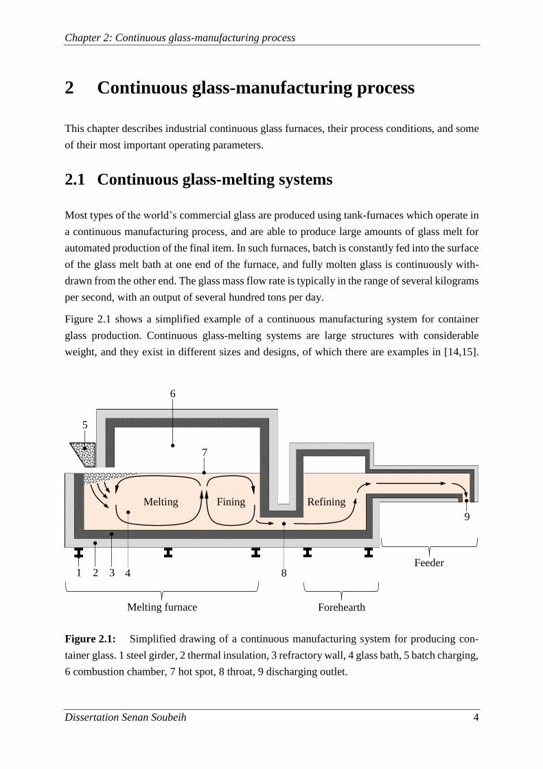
Figure 2.1 shows a simplified example of a continuous manufacturing system for container
glass production. Continuous glass-melting systems are large structures with considerable
weight, and they exist in different sizes and designs, of which there are examples in [14,15].
Figure 2.1: Simplified drawing of a continuous manufacturing system for producing con-
tainer glass. 1 steel girder, 2 thermal insulation, 3 refractory wall, 4 glass bath, 5 batch charging,
6 combustion chamber, 7 hot spot, 8 throat, 9 discharging outlet.
Melting Fining Refining
Feeder
Melting furnace Forehearth
1 2 3
6
7
8
5
4
9
Chapter 2: Continuous glass-manufacturing process
Dissertation Senan Soubeih 5
The system illustrated consists of a melting furnace, a forehearth, and feeders. For the construc-
tion, refractory bricks, mostly of the fused cast alumina-zirconia-silica (AZS) type, are used
[16,17]. There is a layer of thermal insulation bricks on the exterior of the furnace to reduce the
wall heat losses. The whole construction stands on supporting steel girders.
The melting furnace, which is where the melting stage takes place, is a large tank with an inte-
grated combustion chamber above. The tank has a capacity of dozens of cubic meters and the
melting surface is dozens of square meters in area. The batch is fed into one or more openings
in the sides of the tank, forming a blanket on the glass melt. The heat fusing the disparate batch
materials is steadily transferred from the combustion chamber to the surface of the glass bath
by radiation and convection. It comes from fossil fuel burners which shoot horizontal flames
above the glass bath surface.
In the melting tank, the first of the three basic processes that take place is thus the melting. The
other two are fining and homogenizing. The melting process is accomplished in the “melting
zone” which extends over about two-thirds of the tank length. In this zone the batch materials
are completely fused and dissolved, so that the melting process which begins when the batch
enters the melting tank is completed when the glass melt becomes batch-free. The freshly mol-
ten glass contains numerous gaseous bubbles. These are removed by the fining process in which
the bubbles rise to the glass bath surface and escape into the combustion space. This process is
accomplished in the “fining zone” which is the last third of the melting tank. The homogenizing
process, accomplished in the whole tank, is the thorough mixing of the molten glass to achieve
uniformly distributed temperature throughout the glass melt, which will thus be thermally and
chemically homogenous. In the melting zone, the homogenizing also involves uniformly dis-
tributing the batch components within the melt.
The glass melt obtained leaves the melting tank at a temperature of about 1350 °C, passing to
a “forehearth” through a connecting throat. In the forehearth, the glass melt is slowly cooled
from the necessary melting temperature to a defined temperature. This process allows the re-
maining small gaseous bubbles to dissolve in the glass melt, and is called “refining”. The fore-
hearth is connected to automatic molds by several feeders which are usually ducts. In the feed-
ers, the glass melt cools slowly from the refining temperature to the suitable forming tempera-
ture. The final glass melt product is discharged from the feeder-outlet to the automatic molds
at a certain mass flow rate. Temperature homogenizing is also necessary in the forehearth and
feeders to avoid defects, which can be caused if there are strong temperature gradients within
the glass melt.
Chapter 2: Continuous glass-manufacturing process
Dissertation Senan Soubeih 6
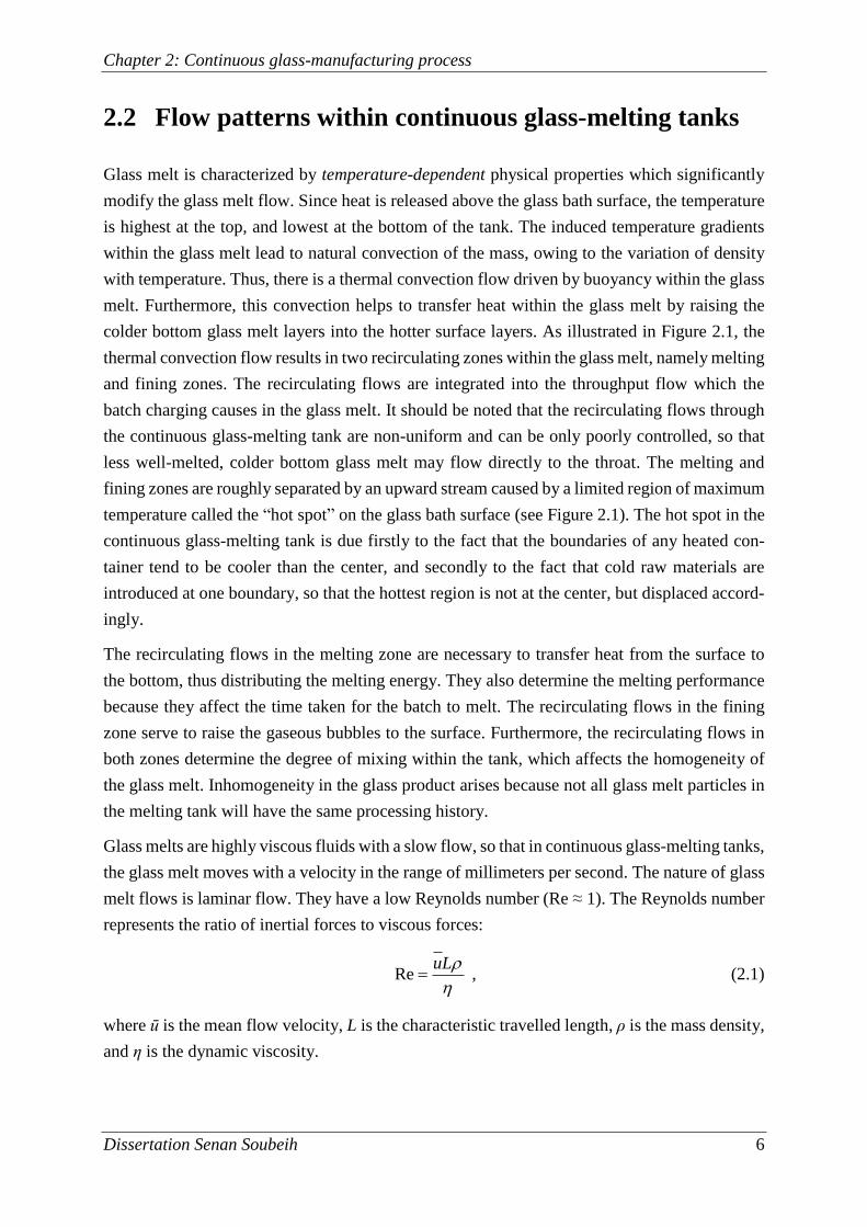
2.2 Flow patterns within continuous glass-melting tanks
Glass melt is characterized by temperature-dependent physical properties which significantly
modify the glass melt flow. Since heat is released above the glass bath surface, the temperature
is highest at the top, and lowest at the bottom of the tank. The induced temperature gradients
within the glass melt lead to natural convection of the mass, owing to the variation of density
with temperature. Thus, there is a thermal convection flow driven by buoyancy within the glass
melt. Furthermore, this convection helps to transfer heat within the glass melt by raising the
colder bottom glass melt layers into the hotter surface layers. As illustrated in Figure 2.1, the
thermal convection flow results in two recirculating zones within the glass melt, namely melting
and fining zones. The recirculating flows are integrated into the throughput flow which the
batch charging causes in the glass melt. It should be noted that the recirculating flows through
the continuous glass-melting tank are non-uniform and can be only poorly controlled, so that
less well-melted, colder bottom glass melt may flow directly to the throat. The melting and
fining zones are roughly separated by an upward stream caused by a limited region of maximum
temperature called the “hot spot” on the glass bath surface (see Figure 2.1). The hot spot in the
continuous glass-melting tank is due firstly to the fact that the boundaries of any heated con-
tainer tend to be cooler than the center, and secondly to the fact that cold raw materials are
introduced at one boundary, so that the hottest region is not at the center, but displaced accord-
ingly.
The recirculating flows in the melting zone are necessary to transfer heat from the surface to
the bottom, thus distributing the melting energy. They also determine the melting performance
because they affect the time taken for the batch to melt. The recirculating flows in the fining
zone serve to raise the gaseous bubbles to the surface. Furthermore, the recirculating flows in
both zones determine the degree of mixing within the tank, which affects the homogeneity of
the glass melt. Inhomogeneity in the glass product arises because not all glass melt particles in
the melting tank will have the same processing history.
Glass melts are highly viscous fluids with a slow flow, so that in continuous glass-melting tanks,
the glass melt moves with a velocity in the range of millimeters per second. The nature of glass
melt flows is laminar flow. They have a low Reynolds number (Re ≈ 1). The Reynolds number
represents the ratio of inertial forces to viscous forces:
LuRe , (2.1)
where ū is the mean flow velocity, L is the characteristic travelled length, ρ is the mass density,
and η is the dynamic viscosity.
Chapter 2: Continuous glass-manufacturing process
Dissertation Senan Soubeih 7
2.3 Residence time distribution (RTD)
Continuous glass-melting tanks are large thermo-chemical reactors with very complex flow
patterns. For adequate processing, the glass melt requires a minimum residence time (MRT)
within the melting tank. This processing includes completely dissolving the raw materials, thor-
oughly mixing the glass melt, and properly degassing it to yield a product that satisfies the
quality standards. MRT is determined by the recirculating flows within the glass-melting tanks.
A very low MRT implies that a part of the glass melt has not had enough time to be completely
melted, thoroughly mixed, and properly degassed. Thus, MRT is an indicative parameter and a
decisive criterion for evaluating glass quality.
Differences in residence time are imposed by the hardly controllable flow patterns within con-
tinuous glass-melting tanks. The glass melt particles travel along an unlimited number of dif-
ferent possible paths between the various positions at the charging opening and the destinations
at the throat. The glass melt particles will also, clearly, have non-uniform recirculating history
through the tank. As travelling along a certain path takes a certain length of time, the different
glass melt particles will spend different lengths of time within the tank. So, each glass melt
particle by following its path will have a particular residence time within the tank. These resi-
dence time differences and variations in the processing time of the glass melt particles cause
inhomogeneity in the glass melt.
An ideal melting cycle (Figure 2.2 (a)) assumes, in a simplified manner, that all glass melt
particles flow uniformly through the tank. Accordingly, if the melting cycle were ideal, all glass
melt particles would have the same residence time within the tank. This uniform residence time
would be equal to the mean residence time τ, which is given by the ratio of the tank space
volume V (glass bath volume) to the volumetric flow rate through the tank V :
V
V
. (2.2)
The slightly recirculated glass melt particles will, clearly, have shorter residence times than the
ideal. Thus, some parts of the glass product will be less-well processed and will be of lower
quality than the average, while excessively recirculated glass parts will have longer residence
times than the ideal and will be responsible for wasted consumption of energy.
The distribution of the lengths of time spent by every glass melt particle within the melting tank
is called “residence time distribution” (RTD). Continuous glass-melting tanks show wide RTD
(see Figure 2.2 (b)). In typical tanks, MRT is between 7% and 15% of the mean residence time
τ. The result is inhomogeneity in the glass melt product. The element of the glass melt with the
MRT has the worst quality.
Chapter 2: Continuous glass-manufacturing process
Dissertation Senan Soubeih 8
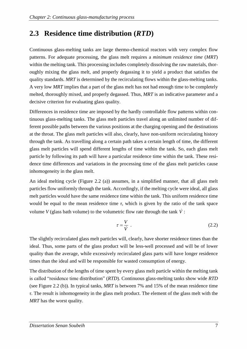
In chemical reaction engineering, RTD is an important parameter for assessing the reactor op-
eration. RTD is usually found by tracer studies, in which an amount of tracer is introduced at
the tank-inlet, and the change in its concentration over time is measured at the tank-outlet. The
RTD transition function (also called the “F curve”) describes the cumulative RTD. The F curve
can be established by plotting the mass fraction rise from zero to unity at the tank-outlet as a
function of time, see Figure 2.2 [18]. In other words, the F curve describes the glass melt par-
ticles leaving the tank as a function of time. Consider a quantity of glass that is introduced at
the tank-inlet at t = 0. The observer is measuring at the tank-outlet. A fraction of the introduced
glass will be observed arriving at the tank-outlet first after an MRT. Then, the fraction arriving
the tank-outlet will continue to increase until the complete glass amount, which represents
unity, has left the tank after a maximum residence time tmax.
The mean residence time τ, which is constant at a constant volumetric flow rate through the
tank (see Equation (2.2)), is represented by the area above the F curve:
max
max
t
MRT
dtt F , (2.3)
with MRT ≤ τ and tmax ≥ τ.
As these mathematical observations reveal, it would be possible significantly to enhance both
glass melt quality and homogeneity by increasing the MRT in continuous glass-melting tanks.
Furthermore, an increase in MRT will be accompanied by a decrease in tmax (see Equation (2.3)),
resulting in a narrower RTD, which means more homogeneous processing of all parts of the
glass melt. An ideal RTD would be attained if MRT = tmax = τ, cf. Figure 2.2 (a) and (b).
Controlling the flow patterns within the glass-melting tanks is a key technique for increasing
MRT and consequently improving RTD, which is one of the glass industry’s primary challenges
and also the main motivation for this thesis.
Figure 2.2: Transition function or F curve describing the cumulative residence time distri-
bution in a reactor: (a) ideal F curve and (b) typical F curve for continuous glass-melting tanks.
F F
t t τ τ
0
1
0
1
MRT
(a) (b)
Area = τ
Area = τ
tmax
Chapter 3: Electric boosting (EB)
Dissertation Senan Soubeih 9
3 Electric boosting (EB)
This chapter turns to the electrically boosted continuous glass-melting tanks which are specific
to the investigation reported in this thesis.
3.1 Flow control in continuous glass-melting tanks
Chapter 2 has already described the complex flow pattern within continuous glass-melting
tanks, and how significantly it affects the melting process. It has also explained how controlling
the glass melt flow within the tank can improve both melting performance and glass quality.
However, glass melt flow in continuous glass-melting tanks is extremely difficult to influence
and can be only poorly controlled. In the glass industry, it is common to apply one or more of
two well-established methods to control the glass melt flow within the continuous glass-melting
tanks. These are bubbling and electric boosting. A description follows.
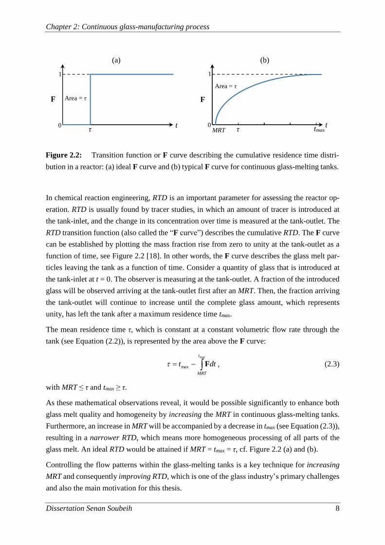
To achieve a certain amount of flow control, the natural convection in continuous glass-melting
tanks is locally enhanced by an additional flow induced near the hot spot location. The addi-
tional flow improves the mixing by raising the colder, less-well melted glass from the bottom
towards the surface. It also intensifies the upward stream which separates the melting and fining
processes. The effect is produced either by “bubbling”, which is blowing air or other gases
through special nozzles installed in the tank bottom near the hot spot location, or by “electric
boosting” which applies direct electric heating to introduce additional heat into the glass bath,
especially near the hot spot location. The electrically generated heat induces an additional ther-
mal convection current within the glass melt, which will bear the bottom glass melt upwards,
see Figure 3.1. The direct electric heating generates Joule heat within the glass melt by using
electrodes. As glass melt is itself a good electrolyte, the electrodes conduct electric currents
directly through it. There is detailed information on the electrochemistry of glass melts in [19–
21]. Although glass in its solid state is a good electrical insulator, it is electrically conducting
when molten, for there is a temperature-dependent increase in electrical conductivity. In gen-
eral, glass melts have an electrical conductivity about five times higher than that of sea water.
Bubbling in comparison with electric boosting has the disadvantage of cooling the glass melt,
while the latter introduces additional heat and intensifies the hot spot. However, both methods
have the disadvantage of exercising only localized influence on the glass melt flow.
As the thesis addresses the use of additional Lorentz forces, the existence of electric current
density within the glass melt is crucial.
Chapter 3: Electric boosting (EB)
Dissertation Senan Soubeih 10
3.2 Continuous glass-melting tanks with barrier booster
For the purposes of the investigation, an industrial continuous glass-melting tank equipped with
an electric boosting system called the “barrier booster” is considered. The barrier booster con-
sists of a rod electrode configuration installed near the hot spot location. The glass bath is thus
heated in the location of the electrodes, so that a thermal barrier is created [22,23], which sup-
ports the hot spot effect and fixes its location. The barrier booster is typically composed of six
rod electrodes introduced into the glass bath vertically through the tank bottom. The boosting
electrodes are spaced evenly in a row across the width of the tank. They are made of molyb-
denum which is the material most compatible with almost all glass types [24,25]. Figures 3.1
and 3.2 provide a schematic representation of the continuous glass-melting tanks that are
equipped with a barrier booster system. It is common to install a barrier wall of refractory ma-
terial behind the barrier booster. This type of continuous glass melting-tank is used for the pro-
duction of container glass. It has a capacity of about 50 m3 and a glass mass flow rate of about
100 T/D (tons per day).
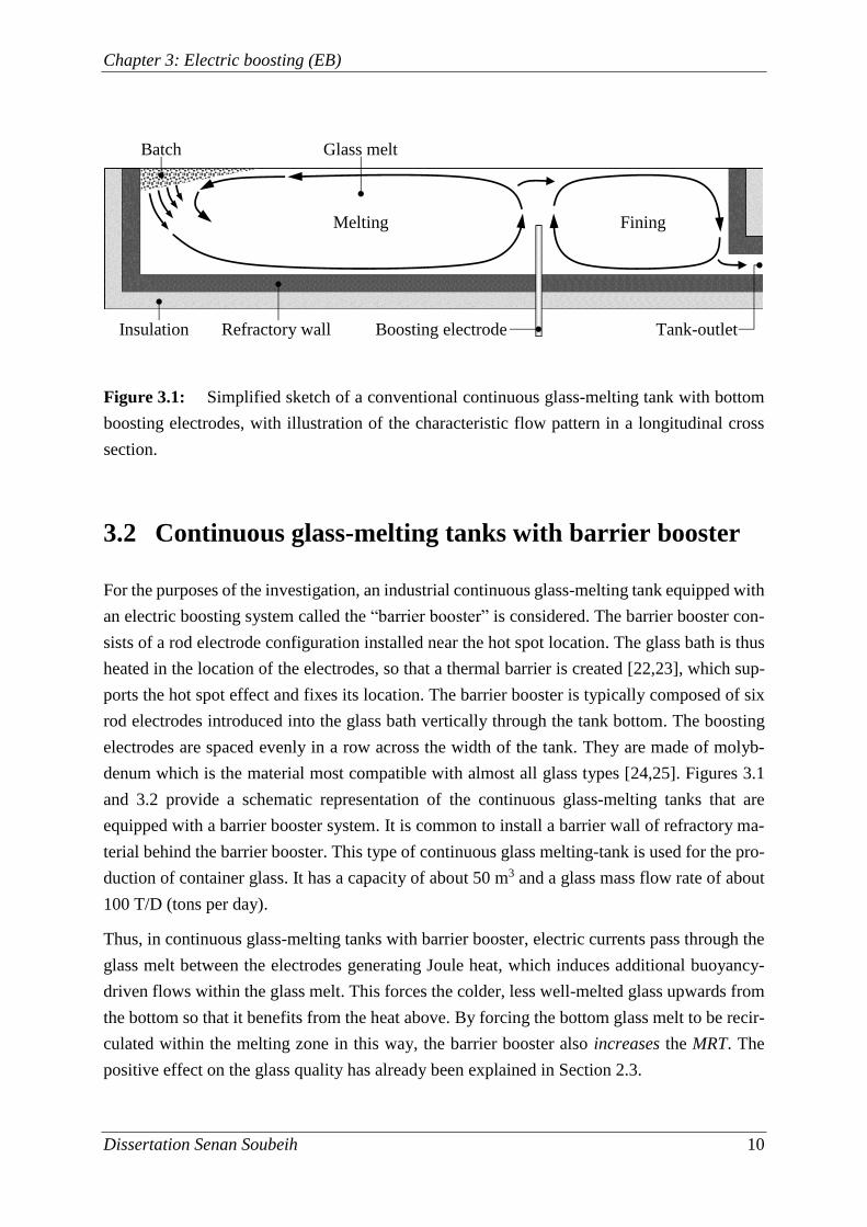
Thus, in continuous glass-melting tanks with barrier booster, electric currents pass through the
glass melt between the electrodes generating Joule heat, which induces additional buoyancy-
driven flows within the glass melt. This forces the colder, less well-melted glass upwards from
the bottom so that it benefits from the heat above. By forcing the bottom glass melt to be recir-
culated within the melting zone in this way, the barrier booster also increases the MRT. The
positive effect on the glass quality has already been explained in Section 2.3.
Figure 3.1: Simplified sketch of a conventional continuous glass-melting tank with bottom
boosting electrodes, with illustration of the characteristic flow pattern in a longitudinal cross
section.
Batch
Melting
Refractory wall
Fining
Insulation Tank-outlet
Glass melt
Boosting electrode
Chapter 3: Electric boosting (EB)
Dissertation Senan Soubeih 11
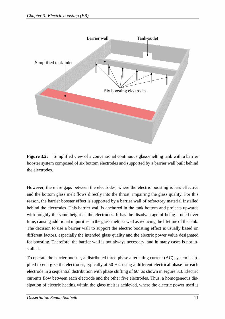
However, there are gaps between the electrodes, where the electric boosting is less effective
and the bottom glass melt flows directly into the throat, impairing the glass quality. For this
reason, the barrier booster effect is supported by a barrier wall of refractory material installed
behind the electrodes. This barrier wall is anchored in the tank bottom and projects upwards
with roughly the same height as the electrodes. It has the disadvantage of being eroded over
time, causing additional impurities in the glass melt, as well as reducing the lifetime of the tank.
The decision to use a barrier wall to support the electric boosting effect is usually based on
different factors, especially the intended glass quality and the electric power value designated
for boosting. Therefore, the barrier wall is not always necessary, and in many cases is not in-
stalled.
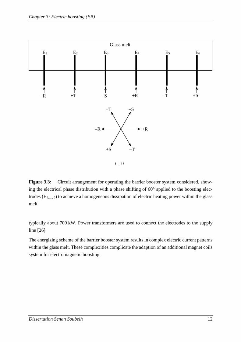
To operate the barrier booster, a distributed three-phase alternating current (AC) system is ap-
plied to energize the electrodes, typically at 50 Hz, using a different electrical phase for each
electrode in a sequential distribution with phase shifting of 60° as shown in Figure 3.3. Electric
currents flow between each electrode and the other five electrodes. Thus, a homogeneous dis-
sipation of electric heating within the glass melt is achieved, where the electric power used is
Figure 3.2: Simplified view of a conventional continuous glass-melting tank with a barrier
booster system composed of six bottom electrodes and supported by a barrier wall built behind
the electrodes.
Tank-outlet Barrier wall
Simplified tank-inlet
Six boosting electrodes
Chapter 3: Electric boosting (EB)
Dissertation Senan Soubeih 12
typically about 700 kW. Power transformers are used to connect the electrodes to the supply
line [26].
The energizing scheme of the barrier booster system results in complex electric current patterns
within the glass melt. These complexities complicate the adaption of an additional magnet coils
system for electromagnetic boosting.
Figure 3.3: Circuit arrangement for operating the barrier booster system considered, show-
ing the electrical phase distribution with a phase shifting of 60° applied to the boosting elec-
trodes (E1,…, 6) to achieve a homogeneous dissipation of electric heating power within the glass
melt.
–R +R –S –T +S +T
Glass melt
–R
+T –S
+R
–T +S
E1 E2 E3 E4 E5 E6
t = 0
Chapter 4: Scope of thesis
Dissertation Senan Soubeih 13
4 Scope of thesis
This chapter states the main substance of this thesis, the concept of electromagnetic boosting in
electrically boosted continuous glass-melting tanks. It also includes a presentation of the aim
and objectives, then concludes with an overview.
4.1 Concept of electromagnetic boosting (EMB)
Electromagnetic boosting (EMB) is a new and innovative approach to improving the flow pat-
terns within the electrically boosted continuous glass-melting tanks. The idea of EMB is to
create a controllable electromagnetic barrier between the boosting electrodes which will hinder
the flow of the bottom glass melt. Furthermore, the electromagnetic barrier, being material-free,
causes no additional impurities in the glass melt, and can replace the traditional barrier wall.
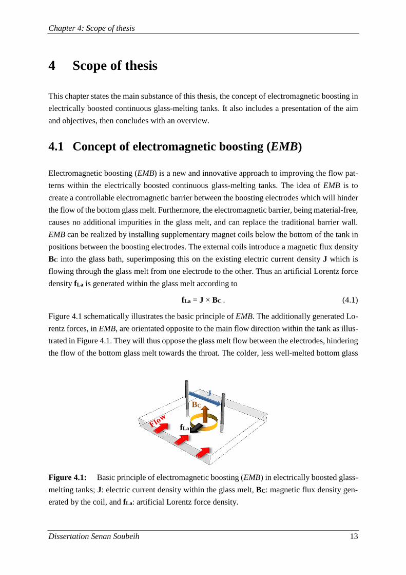
EMB can be realized by installing supplementary magnet coils below the bottom of the tank in
positions between the boosting electrodes. The external coils introduce a magnetic flux density
BC into the glass bath, superimposing this on the existing electric current density J which is
flowing through the glass melt from one electrode to the other. Thus an artificial Lorentz force
density fLa is generated within the glass melt according to
fLa = J × BC . (4.1)
Figure 4.1 schematically illustrates the basic principle of EMB. The additionally generated Lo-
rentz forces, in EMB, are orientated opposite to the main flow direction within the tank as illus-
trated in Figure 4.1. They will thus oppose the glass melt flow between the electrodes, hindering
the flow of the bottom glass melt towards the throat. The colder, less well-melted bottom glass
Figure 4.1: Basic principle of electromagnetic boosting (EMB) in electrically boosted glass-
melting tanks; J: electric current density within the glass melt, BC: magnetic flux density gen-
erated by the coil, and fLa: artificial Lorentz force density.
J
BC
fLa
Chapter 4: Scope of thesis
Dissertation Senan Soubeih 14
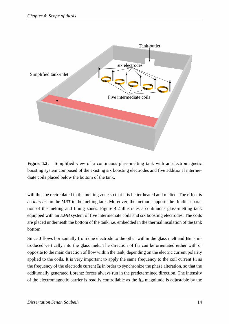
will thus be recirculated in the melting zone so that it is better heated and melted. The effect is
an increase in the MRT in the melting tank. Moreover, the method supports the fluidic separa-
tion of the melting and fining zones. Figure 4.2 illustrates a continuous glass-melting tank
equipped with an EMB system of five intermediate coils and six boosting electrodes. The coils
are placed underneath the bottom of the tank, i.e. embedded in the thermal insulation of the tank
bottom.
Since J flows horizontally from one electrode to the other within the glass melt and BC is in-
troduced vertically into the glass melt. The direction of fLa can be orientated either with or
opposite to the main direction of flow within the tank, depending on the electric current polarity
applied to the coils. It is very important to apply the same frequency to the coil current IC as
the frequency of the electrode current IE in order to synchronize the phase alteration, so that the
additionally generated Lorentz forces always run in the predetermined direction. The intensity
of the electromagnetic barrier is readily controllable as the fLa magnitude is adjustable by the
Figure 4.2: Simplified view of a continuous glass-melting tank with an electromagnetic
boosting system composed of the existing six boosting electrodes and five additional interme-
diate coils placed below the bottom of the tank.
Five intermediate coils
Tank-outlet
Simplified tank-inlet
Six electrodes
Chapter 4: Scope of thesis
Dissertation Senan Soubeih 15
BC magnitude (see Equation (4.1)). Hence, the external control parameter for EMB is the elec-
tric current passed through the coils IC. The desired EMB effect would be an increase in the
MRT and consequently improving of the RTD, and finally an enhancement of the glass quality.
4.2 Aim and objectives of the thesis
It is the author’s aim in this thesis to present his numerical realisation of electromagnetic boost-
ing (EMB) in a continuous glass-melting tank, together with an assessment of the EMB effects,
so as to lay the foundation for converting the idea into an effective industrial process.
This is a challenging aim because a highly complex three-dimensional problem is involved. In
its solution, it is necessary to pursue five objectives.
The first objective is to derive a simplified representation of the actual glass-melting furnace as
the basis for an academic numerical model. This necessitates deriving the mathematical model
that describes the three-dimensional problem considered. The industrially available numerical
models of actual continuous glass-melting tanks comprise the melting tank model with addi-
tional sub-models for the batch melting and combustion chamber. A combination of several
special purpose software packages is used. However, for this academic investigation it is more
useful to consider a tank model with simplified boundary conditions to reduce the simulation
complexities. This approach serves the goal of the model, which is to investigate the pure EMB
effects and study certain parameters by which the system can be analyzed and optimized.
The second objective is to develop a reliable numerical methodology for coupling the electro-
magnetic, flow, and temperature fields. The mathematical model of the problem considered
involves the conservation laws of momentum, mass, and energy. It also involves the governing
equations of the electromagnetic aspect. The necessity for strong coupling of the calculations
arises from the temperature-dependent glass properties. The dynamic viscosity η(T) and mass
density ρ(T) of molten glass decrease with temperature, while the electrical conductivity κ(T)
increases with temperature. Furthermore, the temperature dependence of η(T) and κ(T) is non-
linear. Thus, the temperature distribution within the glass melt T(x,y,z) determines the localized
value of the electrical conductivity of the glass melt κ(T), which, in turn, determines the Lorentz
force density distribution fL(x,y,z) as well as the electric current density distribution J(x,y,z)
within the glass melt. The Lorentz force density distribution affects the glass melt flow, i.e. the
velocity distribution u(x,y,z), which, in turn, has an important influence on the temperature dis-
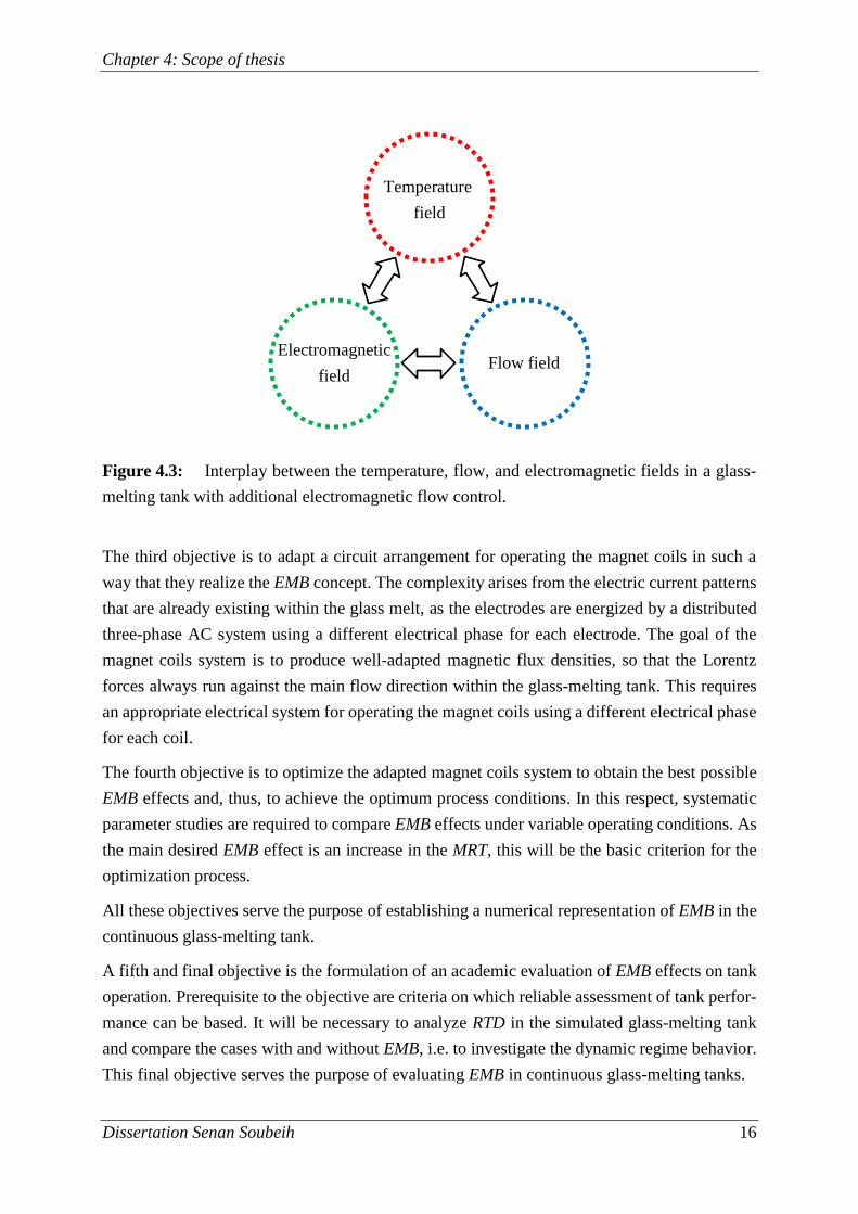
tribution within the glass melt. Figure 4.3 illustrates how the three fields interplay in a closed
loop. As the underlying nonlinear system of governing equations is strongly coupled, it be-
comes necessary to employ a reliable numerical methodology that can effectively solve the
coupled nonlinear three-dimensional problem.
Chapter 4: Scope of thesis
Dissertation Senan Soubeih 16
The third objective is to adapt a circuit arrangement for operating the magnet coils in such a
way that they realize the EMB concept. The complexity arises from the electric current patterns
that are already existing within the glass melt, as the electrodes are energized by a distributed
three-phase AC system using a different electrical phase for each electrode. The goal of the
magnet coils system is to produce well-adapted magnetic flux densities, so that the Lorentz
forces always run against the main flow direction within the glass-melting tank. This requires
an appropriate electrical system for operating the magnet coils using a different electrical phase
for each coil.
The fourth objective is to optimize the adapted magnet coils system to obtain the best possible
EMB effects and, thus, to achieve the optimum process conditions. In this respect, systematic
parameter studies are required to compare EMB effects under variable operating conditions. As
the main desired EMB effect is an increase in the MRT, this will be the basic criterion for the
optimization process.
All these objectives serve the purpose of establishing a numerical representation of EMB in the
continuous glass-melting tank.
A fifth and final objective is the formulation of an academic evaluation of EMB effects on tank
operation. Prerequisite to the objective are criteria on which reliable assessment of tank perfor-
mance can be based. It will be necessary to analyze RTD in the simulated glass-melting tank
and compare the cases with and without EMB, i.e. to investigate the dynamic regime behavior.
This final objective serves the purpose of evaluating EMB in continuous glass-melting tanks.
Figure 4.3: Interplay between the temperature, flow, and electromagnetic fields in a glass-
melting tank with additional electromagnetic flow control.
Electromagnetic
field Flow field
Temperature
field
Chapter 4: Scope of thesis
Dissertation Senan Soubeih 17
4.3 Overview of the thesis
This thesis with its numerical simulation provides the groundwork for the use of the novel and
innovative EMB approach to improve the RTD in electrically boosted continuous glass-melting
tanks. In the simulation, an additional magnet coils system is adapted and assumed to be in-
stalled into the tank to generate additional Lorentz forces within the glass melt. These forces
act against the main flow direction of the glass melt in the tank. The influence of the additionally
generated Lorentz forces on the RTD in a continuous glass-melting tank is systematically stud-
ied using three-dimensional numerical simulations based on the geometry of a real industrial
glass-melting tank. Furthermore, the physical properties of soda-lime glass are taken into ac-
count: the temperature dependence of the electrical conductivity, the dynamic viscosity, and
the mass density. The tank performance with and without EMB is compared, to investigate the
feasibility of EMB in continuous glass-melting tanks. The optimum operating conditions are
also sought with a view to optimizing the EMB.
The literature on the subject is referred to in Chapter 5. The literature draws its relevance from
two aspects, namely numerical simulation of glass-melting tanks and Lorentz forces in glass
manufacture. Both aspects lead to useful conclusions and possible approaches.
Following the literature review, Chapter 6 presents the model for the tank under consideration,
deriving therefrom the appropriate mathematical model. This describes the physical phenomena
which characterize the operation of the tank. It also defines the real three-dimensional problem
by means of a system of equations.
Chapter 7 presents the numerical methodology employed to couple the calculations. Calcula-
tions of simplified examples to validate and test the method are also provided in this chapter.
The methodology adapted is to include the electromagnetic field calculation in software which
was developed for calculating coupled hydrodynamic and thermodynamic effects, the commer-
cial program FLUENT. This numerical methodology was first applied in [27] with highly sim-
plified considerations, which were later systematically developed to the complete system in
[28–31]. In these developments, the author was a member of the investigative team.
In Chapter 8, the author presents details of the computational grid, followed by a discussion of
the numerical solution for the governing equations. The chapter concludes with different sys-
tematic studies by which the numerical accuracy is verified.
The numerical simulation of the actual continuous glass-melting tank is the subject of Chap-
ter 9. The boundary conditions are so defined as to simulate the realistic conditions in the tank.
The chapter also contains a determination of the circuit arrangement for operating the magnet
coils so as to realize the EMB concept. There are parameter studies to establish the optimum
process conditions. The simulation results are thoroughly discussed and comparisons are made,
indicating a fruitful investigation. In the last section of Chapter 9, an additional fact is taken
Chapter 4: Scope of thesis
Dissertation Senan Soubeih 18
into account: the structural steel of the tank construction. This is relevant to the installation of
additional magnet coils. The fact that the magnetic field is generated near steel construction
elements requires exploration.
The last chapter, Chapter 10, presents the conclusions and outlook.
The work and its main results have been published at events in [32–34] and in a peer-reviewed
international scientific journal [35]. The tank simulations and their results have also been pre-
sented, discussed and published at specialized conferences of the international glass industry
[36–38] and at the specialized conference on ANSYS numerical simulation [39].
Chapter 5: Literature, state of the art
Dissertation Senan Soubeih 19
5 Literature, state of the art
Here follows a comprehensive survey of the literature on subjects that are relevant to the present
work. The literature falls into two groups, namely that relating to numerical simulation of glass-
melting tanks and that on Lorentz forces in glass manufacture. The author draws the content
into a presentation of the state of the art in each field.
5.1 Numerical simulation of glass-melting tanks
There is constant demand for better glass quality and lower glass processing costs. The demand
can only be met by full insight into the glass melting process. Numerical simulation is already
a tried and trusted tool in the glass industry. With the advent of the computer in the second half
of the 20th century, mathematical models could come into practical use for glass-melting tanks.
The evolution of simulation tools which have been used to model glass-melting furnaces is
outlined in [40]. An overview of mathematical modeling in glass manufacture is presented in
[41–43]. The report on mathematical modeling in glass processing in [44] is particularly useful.
The most influential papers on numerical simulation of glass-melting tanks are reviewed in the
following.
Curran [45] did pioneering work in 1971. He formulated a two-dimensional computer model to
study various electrode configurations in a hypothetical all-electric tank-furnace. Curran used
contour maps in his work to visualize the isotherms and streamlines, and this is still the main
means of presenting results today. This two-dimensional simulation was followed by another
work of Curran [46], in which he studied the effects of various glass colors. He used Rosseland
approximation to derive an effective thermal conductivity for the glass melt, which has been
successfully employed ever since. Additional progress in the two-dimensional models came
when Austin & Bourne [47], followed by Leyens [48], Mase & Oda [49], and Mardorf & Woelk
[50] included the calculation of the batch feeding and melting.
Leyens & Smrček [51] studied the effects of the feeding rate and tank depth on RTD, while the
papers published by Leyens et al. [52] and Nolet [53] included tracer studies performed on
operating furnaces to compare the RTD with the predictions of two-dimensional mathematical
models. Indeed, they found good agreement.
An early attempt at a three-dimensional numerical model of glass-melting furnaces was made
by Chen & Goodson [54] in 1972. Their purpose was only to develop an efficient computational
approach, using a highly simplified furnace model, as the limits of computational capacities at
that time restricted the computation of realistic three-dimensional models for glass-melting fur-
Chapter 5: Literature, state of the art
Dissertation Senan Soubeih 20
naces. With the advent of commercial powerful computers in the early 1980’s, it became pos-
sible to use three-dimensional models for analyzing glass process. The newly established
method was employed to study a variety of glass furnace problems. An early three-dimensional
study by Moult [55] concentrated on the throat region of the glass-melting furnace. Simonis et
al. [56] considered the influences of the glass flow rate, of bubbling, and of electric boosting.
Ungan & Viskanta [57,58] developed a coupling of the combustion, batch melting, and tank
models. They also used their coupled models to study the effects of electric boosting and air
bubblers in the glass-melting furnace. Choudhary [59,60] developed a three-dimensional model
and with it studied an all-electric furnace. While Ghandakly & Curran [61] developed a tech-
nique to model the electrical resistances between the electrodes in electric glass-melting fur-
naces. Murnane et al. [62] analyzed a variety of glass processing problems. Further papers [63–
68] also appeared in the field of mathematical modeling of industrial glass-melting furnaces.
The various authors of these papers addressed the control of the glass melt flow by evaluating
the effects of bubbling, electric boosting, barrier wall, natural convection, and electrode ar-
rangements. In other papers, for instance [69], the energy balance in glass-melting furnaces was
described. Gopalakrishnan et al. [70] investigated time-dependent electrode energizing to im-
prove the mixing in an all-electric glass-melting furnace.
In order to establish a benchmark test for the modeling of glass-melting tanks, the Technical
Committee 21 (TC 21) of the International Commission on Glass (ICG) ran the first Round
Robin Test (RRT1), in which a very simplified glass-melting tank was considered. The purpose
was to test tank simulation codes by comparing the calculated velocity distributions, tempera-
ture distributions, and MRT’s. The results submitted by the participants were compared and
published by Muschick & Muysenberg [71]. Moukarzel et al. [72] recalculated the RRT1 using
the commercial software FLUENT, and demonstrated the importance of numerical precision
for MRT calculation.
Many of the publications discussed the calculation and analysis of RTD in glass-melting tanks.
The authors of [56,60], obtained the RTD by simulating a tracer experiment. This method was
found to have the disadvantage of slow calculation and low accuracy. An alternative powerful
method that involves performing particle tracing was applied in [64,65,72,73]. This method
was found quick and accurate and, furthermore, able to provide information on MRT and parti-
cle path. In the last decades, the validation of mathematical models using data of operating
glass-melting tanks has often been the subject of papers and has shown that the results reason-
ably agree with practical observations. The authors are agreed that qualitatively good predic-
tions are attainable from numerical simulation, see [52,53,65,68,74–76].
Conclusions drawn from numerical simulation of glass-melting tanks
Today’s mathematical models, as is shown in the progression recounted above, are becoming
more accurate than physical models to simulate glass-melting tanks and they are replacing them
Chapter 5: Literature, state of the art
Dissertation Senan Soubeih 21
increasingly. This arises from their ability to use the real glass material properties which are
usually provided by measurements, and to address the real processing conditions in the furnace.
Numerical simulation using CFD models is shown in the literature to be a reliable tool for op-
timizing the operating parameters of the glass-melting tank, predicting glass quality, and eval-
uating new configurations and designs. The calculation technique most often applied is the Fi-
nite Volume Method (FVM), which is widely available in such commercial software programs
as FLUENT. So far, there is no simulation tool that completely covers all processes in glass
technology. Hence, in the literature, the CFD models are linked with additional sub-models to
include the calculations of combustion and batch melting processes, using thus several special
purpose software packages. For purposes of better control of the flow of the glass melt, numer-
ical simulation has been used to study the effects of natural convection, bubbling, electric boost-
ing, and electrode arrangements. The importance of MRT as a critical parameter for evaluating
glass quality has also been emphasized in the literature by authors who studied and analyzed
RTD to understand the flow behavior within the tank and to evaluate the tank performance. The
particle tracing technique, as also reported in the literature, offers a reliable and powerful nu-
merical method to calculate RTD and to provide the particle path and MRT.
5.2 Lorentz forces in glass manufacture
Two types of Lorentz forces are known in glass manufacture, and are distinguished by their
origin. The one type occurs naturally in directly electrically heated glass melts, and is referred
to as “natural Lorentz force”. The other type is artificially imposed on the electrically heated
glass melts to obtain control of the flow, and is referred to as “artificial Lorentz force”.
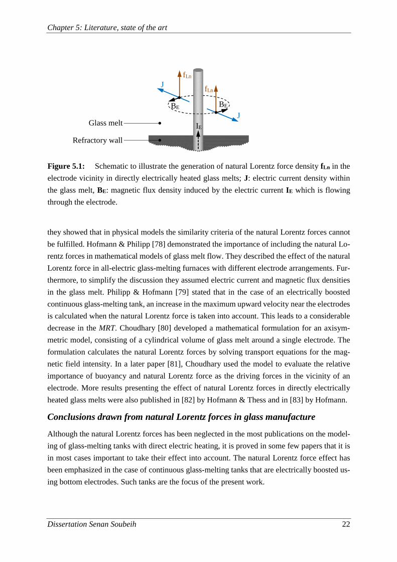
5.2.1 Natural Lorentz forces
When glass melt is electrically heated using rod electrodes, Lorentz force densities arise natu-
rally in the vicinity of the heating electrode. The natural Lorentz force density fLn is induced
when the radial electric current density J, which is flowing from the electrode into the glass
melt, interacts with the magnetic flux density BE called “eigenfield” which is induced by the
electric current passing through the electrode itself:
fLn = J × BE. (5.1)
As illustrated in Figure 5.1, the natural Lorentz forces always run towards the tip of the elec-
trode, causing an extra flow component in the tiny area surrounding the electrode.
The contribution of natural Lorentz forces as a flow component was initially neglected in the
computations of flow and heat transfer in electrically heated glass melts. However, in 1991,
Hofmann & Kaliski [77] indicated the importance of considering natural Lorentz forces as a
second driving force beside buoyancy in the immediate vicinity of the electrodes. Moreover,
Chapter 5: Literature, state of the art
Dissertation Senan Soubeih 22
they showed that in physical models the similarity criteria of the natural Lorentz forces cannot
be fulfilled. Hofmann & Philipp [78] demonstrated the importance of including the natural Lo-
rentz forces in mathematical models of glass melt flow. They described the effect of the natural
Lorentz force in all-electric glass-melting furnaces with different electrode arrangements. Fur-
thermore, to simplify the discussion they assumed electric current and magnetic flux densities
in the glass melt. Philipp & Hofmann [79] stated that in the case of an electrically boosted
continuous glass-melting tank, an increase in the maximum upward velocity near the electrodes
is calculated when the natural Lorentz force is taken into account. This leads to a considerable
decrease in the MRT. Choudhary [80] developed a mathematical formulation for an axisym-
metric model, consisting of a cylindrical volume of glass melt around a single electrode. The
formulation calculates the natural Lorentz forces by solving transport equations for the mag-
netic field intensity. In a later paper [81], Choudhary used the model to evaluate the relative
importance of buoyancy and natural Lorentz force as the driving forces in the vicinity of an
electrode. More results presenting the effect of natural Lorentz forces in directly electrically
heated glass melts were also published in [82] by Hofmann & Thess and in [83] by Hofmann.
Conclusions drawn from natural Lorentz forces in glass manufacture
Although the natural Lorentz forces has been neglected in the most publications on the model-
ing of glass-melting tanks with direct electric heating, it is proved in some few papers that it is
in most cases important to take their effect into account. The natural Lorentz force effect has
been emphasized in the case of continuous glass-melting tanks that are electrically boosted us-
ing bottom electrodes. Such tanks are the focus of the present work.
Figure 5.1: Schematic to illustrate the generation of natural Lorentz force density fLn in the
electrode vicinity in directly electrically heated glass melts; J: electric current density within
the glass melt, BE: magnetic flux density induced by the electric current IE which is flowing
through the electrode.
IE
fLn
J
BE
fLn
BE
J Glass melt
Refractory wall
Chapter 5: Literature, state of the art
Dissertation Senan Soubeih 23
5.2.2 Artificial Lorentz forces
While flow control using Lorentz forces is a widely applied technology in many metallurgical
processes, no use of Lorentz forces in glass manufacture has yet become established. The dif-
ficulty arises from the relatively small electrical conductivity of molten glass (about five orders
of magnitude less than molten metals). Therefore, in glass processing, the essential effect of
electric current is to generate Joule heat within the glass melt. However, a number of proposals
has been made for applying artificial Lorentz force in glass manufacture. A review follows.
There is a patent registered as early as 1932 by Bates & Haskell [84]. The inventors suggest a
method for controlling the successive delivery of molten glass to forming device using artificial
Lorentz forces. Furthermore, the orientation of artificial Lorentz forces is alternated to either
accelerate or retard the glass melt flow through a feeder discharge passage. The inventors sug-
gest two arrangements of annular coils with iron frames for the magnetic circuit. For the coil
arrangements they suggest a two-phase winding and a distributed three-phase winding, for
which they give a detailed switching diagram. According to the suggested method, the gener-
ated magnetic flux density will induce electric current density within the glass melt. However,
at the suggested low frequency of 60 Hz, the induced electric currents cannot be expected to
have the desired effect, because molten glass has such low electrical conductivity. Therefore,
in this author’s eyes, the method remains doubtful. Moreover, the patent lacks the operation
requirements, i.e. the setup dimensions and the magnitudes of magnetic flux density and in-
duced electric current density.
Forty years later, in 1972, Walkden [85] patented a method for homogenizing glass melts using
artificial Lorentz forces. The given method relates to the glass melts that are electrically heated
using electrodes, mainly in forehearths and all-electric furnaces. The inventor suggests different
arrangements of electromagnets connected in series with the heating electrodes. The electro-
magnets are thus energized by the same electric current as the electrodes, using either a single-
phase or a three-phase alternating current system at 50 Hz. The patent schematically describes
different glass melt flow patterns obtained in a forehearth that is equipped with three heating
electrodes and two additional intermediate electromagnets.
In 1981, Mikelson et al. [86] patented an arrangement for refining and homogenizing optical
glasses in crucibles using artificial Lorentz forces. In this case, the arrangement consists in three
pairs of electrodes and two electromagnets. The electrodes pass alternating electric current
through the glass melt, and the electromagnets introduce alternating magnetic flux density into
it. The electric current is sequentially changed in three directions that are perpendicular to each
other. Simultaneously, the magnetic field is changed in two directions that are perpendicular to
each other and to the electric current. The inventors propose a specific glass melt flow regime,
which rotates the glass melt in three planes that are perpendicular to each other. The active
plane alternates every few seconds according to the switching sequence that is applied to the
Chapter 5: Literature, state of the art
Dissertation Senan Soubeih 24
electric current and magnetic field. Osmanis et al. [87] obtained a further patent in which an
additional suggestion is given. Here an additional high-frequency magnetic field is applied to
generate vibrations in the glass melt.
Fekolin & Stupak [88] report on physical model based on the similarity theory to investigate
the electromagnetic stirring in electrically heated feeders. The model comprises a channel, an
electrode arrangement, an electromagnet, and a glycerin-based model liquid. The authors study
the dependence of the liquid’s maximum velocity in the stirring zone on the magnetic flux
density magnitude at different electric currents applied to the electrodes. However, as the sim-
ilarity criteria of the temperature-dependent material properties are not considered, results from
such a model remains doubtful.
A theoretical view of the application of Lorentz force in glass melts has been published by
Hofmann & Thess [82]. They provide an overview of the magnetohydrodynamic effects and
highlight the potential for controlling glass melt flow. A later computed example is given by
Hofmann in [83].
A method using artificial Lorentz forces to control the glass melt mass flow rate in feeders was
patented in 2005 by Kunert et al. [89]. According to this method, the artificial Lorentz forces
are orientated either in or opposite to the glass melt flow direction. This will either accelerate
or decelerate the glass melt flow in the feeder channel. The inventors suggest introducing an
electric current and a magnetic field simultaneously into the glass melt. These fields are per-
pendicular to each other and both are perpendicular to the flow direction. The concept of elec-
tromagnetically controlled mass flow rate in feeder channels has been further investigated by
Giessler et al. [90–92] using a simplified representation of the system. They consider a pipe
with circular cross-section to study the effects of artificial Lorentz forces on temperature distri-
bution and velocity. To simplify the study, they use a one-dimensional analytical model [90],
and validate the results by two-dimensional axisymmetric numerical simulations [91].
A first demonstration of how artificial Lorentz forces can be effectively used to stir and homog-
enize the glass melts in a crucible is given by Hülsenberg et al. [93] and Krieger et al. [94,95].
They use a laboratory-scale cylindrical crucible, in which two electrodes are immersed in the
glass melt to introduce electric current. Furthermore, a magnetic flux density that is perpendic-
ular to the electric current density is introduced to the glass melt using an external magnet sys-
tem. Thus, artificial Lorentz forces are generated, of which the direction can be changed ac-
cording to the magnetic field and electric current directions. The authors show, by experimental
studies, how artificial Lorentz forces enhance both thermal and chemical homogeneity of the
glass melt. The experimental measurements of temperature distribution within the glass melt
are then compared with numerical results by Cepite et al. [96]. The crucible setup is also used
Chapter 5: Literature, state of the art
Dissertation Senan Soubeih 25
by Giessler et al. [92,97–99], who study the relations between velocity, temperature, and artifi-
cial Lorentz force. They formulate a simple one-dimensional analytical model in [97,98], and
perform three-dimensional numerical simulations in [99].
In 2007, Halbedel et al. [100] patented a method for electromagnetically stirring and homoge-
nizing technical glasses within the discharging channel. The inventors suggest an arrangement
composed of inner and outer cylindrical electrodes enclosed by a magnet coil system. The glass
discharging channel, which is an electrically conducting pipe with circular cross-section, con-
stitutes the outer electrode. The inner electrode is a rod inserted axially into the channel. The
radial electric current density within the glass melt interacts with the axial magnetic flux density
generated by the coils. Thus artificial Lorentz forces are generated perpendicular to the flow
direction.
Two years later, Hofmann [101] gives in his patent a method for electromagnetically mixing,
degassing, and homogenizing the electrically heated glass melts. The inventor suggests apply-
ing unequal frequencies for each electric current and magnetic field, thus obtaining artificial
Lorentz forces that change their direction. According to the difference value between the ap-
plied frequencies, the artificial Lorentz forces change their direction at longer or shorter inter-
vals so that the mixing behavior will be appropriate either to degassing or to homogenizing.
Gopalakrishnan & Thess [102] report on their numerical investigation of an electromagnetic
pipe mixer which is proposed for homogenizing optical glasses. The mixer is composed of an
electrically conducting pipe, two inner rod electrodes energized alternately, and surrounding
coils which generate an axial magnetic flux density. Another evaluation including validation
by a physical model is given by Torres & Halbedel [103].
In his thesis for the German Diplom, Kelm [104] describes three-dimensional numerical simu-
lations that are related to the EMB concept. The simulations are carried out for a simple ar-
rangement composed of a magnet coil placed between two rod electrodes that are immersed in
a glass melt cube. A single-phase alternating current system at 50 Hz is assumed for the elec-
trodes and coil. Furthermore, constant glass material properties are assumed. The temperature
effect and gravity term are not considered in the simulations. Kelm investigates the basic influ-
ence of artificial Lorentz forces on the glass melt flow between two boosting electrodes. The
natural Lorentz forces are considered in the simulations. First, the electromagnetic field is cal-
culated by the commercial software MAXWELL. The calculated Lorentz force densities are
then exported into the commercial software FLUENT to perform the flow field calculations.
There is a recent addition to the literature by Torres et al. [105], who investigate the artificial
Lorentz force application to improve the glass coloring process in forehearths. They propose an
arrangement composing three rod electrodes and two magnet coils. Both are energized with a
single-phase alternating current system at 50 Hz. The coils are placed underneath the forehearth
refractory bottom in positions between the electrodes which are introduced into the glass melt
Chapter 5: Literature, state of the art
Dissertation Senan Soubeih 26
through the forehearth bottom. The artificial Lorentz forces are orientated in the opposite di-
rection to the glass melt flow to induce an upward push. This improves the mixing conditions
in the forehearth, ultimately resulting in a better color homogenizing process.
Conclusions drawn from artificial Lorentz forces in glass manufacture
From this comprehensive survey of the fairly limited number of publications in the field, it is
concluded that Lorentz force application to control glass melt flow is still in its infancy. Some
attention has been given to homogenizing the glass melt and controlling the glass melt mass
flow rate using artificial Lorentz forces. Furthermore, a variety of setups has been proposed for
different glass compositions. The control parameters have been the magnetic flux density, elec-
tric current density, and frequency. The investigations have been accomplished by experimental
studies, physical models and numerical simulations. The published results have demonstrated
the effective application of artificial Lorentz force to control glass melt flow, which provides a
contactless method. However, there has been no investigation to date of other potential appli-
cations that are related to artificial Lorentz forces in glass melts, such as the improvement of
RTD in continuous glass-melting tanks. The current work attempts to remedy this.
Chapter 6: Problem formulation
Dissertation Senan Soubeih 27
6 Problem formulation
This chapter presents the system under consideration and derives the governing equations to
describe the three-dimensional problem in mathematical terms.
6.1 Tank representation
The author’s work takes for its academic purposes a simplified model of an industrial-scale
glass-melting tank used to produce container glass. The model is illustrated in Figure 4.2 and
the dimensions are shown in Figures 6.1 and 6.2. The tank walls are assumed to have a uniform
thickness that is equal to the sum of the thickness of the refractory and of the thermal insulation
(each is assumed to be 200 mm). An equivalent thermal conductivity is assumed for the tank
walls. A simplified tank-inlet is used for the numerical simulation. The model here applied takes
a tank-inlet that is a bounded surface on the glass melt bath. The complicated chemical reactions
and heat transfer within the batch are not included in the model, and the batch is assumed to be
molten glass that has a constant mass flow rate with a prescribed temperature at the simplified
tank-inlet.
The tank is equipped with an electric boosting system composed of six molybdenum electrodes
installed through the tank bottom. The boosting electrodes are operated by a three-phase AC
system at 50 Hz, using a different electrical phase for each electrode, as shown in Figure 3.3.
The electric boosting system introduces a specified amount of electric power into the glass melt,
which provides additional heating near the electrodes. In the model, no barrier wall is consid-
ered as the purpose is to study the pure EMB effects, and to compare the dynamic regime be-
havior with and without EMB. Furthermore, a case that considers the barrier wall cannot serve
as a baseline for comparison with EMB case in which the barrier wall is essentially discarded,
the comparison would not be of like with like.
The EMB system considered comprises five intermediate coils in addition to the six boosting
electrodes, as shown in Figure 6.2. The coils are considered to be placed 200 mm under the
glass melt, i.e. in the thermal insulation directly under the refractory bottom. With an outer
diameter of 600 mm, the coils can be assumed to cover the area in which EB is less effective.
In practice, the coils can be made of a copper conductor cooled by passing water through a gap
inside the conductor itself. In this thesis, a square cross section with 10 mm side length is as-
sumed for the copper conductor. 20 turns are assumed for each coil, making the coil height
200 mm in total.
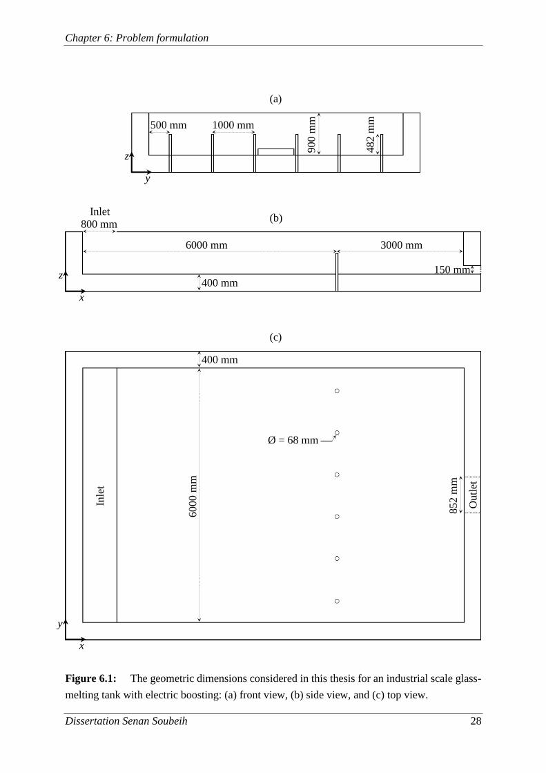
Chapter 6: Problem formulation
Dissertation Senan Soubeih 28
Figure 6.1: The geometric dimensions considered in this thesis for an industrial scale glass-
melting tank with electric boosting: (a) front view, (b) side view, and (c) top view.
y
z
x
z
x
y
150 mm
800 mm
6000 mm 3000 mm
482 m
m
400 mm
500 mm 1000 mm
852 m
m
6000 m
m
400 mm
Ø = 68 mm
Inle
t
Inlet
Outl
et
(a)
(b)
(c)
900 m
m

Chapter 6: Problem formulation
Dissertation Senan Soubeih 29
Figure 6.2: The coil dimensions and locations considered for the EMB system: (a) front
view, (b) side view, and (c) top view. E1,…, 6 and C1,…, 5 are the electrodes and coils respectively.
y
z
x
z
x
y
200 mm
Ø = 600 mm
Inlet
600 mm
(a)
(b)
(c)
Outlet
E1
E2
E3
E4
E5
E6
C1
C2
C4
C5
C3
Chapter 6: Problem formulation
Dissertation Senan Soubeih 30
6.2 Mathematical model
The mathematical model involves the equations governing the electromagnetic aspect, the glass
melt flow, and the transfer of heat.
6.2.1 Glass material properties
To start with the nature of glass itself, the soda-lime glass composition known as “DGG-Stand-
ardglas Ia” [106], whose physical properties have been measured experimentally, is assumed.
The glass melt has a very high dynamic viscosity η(T) which decreases nonlinearly with tem-
perature T. Furthermore, η(T) is approximated on the base of Vogel-Fulcher-Tammann equation
[13] using the logarithmic function
T
BAT )(log , (6.1)
where A and B are constants pertaining to the glass composition.
The mass density ρ(T) of the glass melt decreases with temperature T, and is considered to obey
the linear approximation:
ρ(T) = – aT + b, (6.2)
where the constants a and b also pertain to the glass composition.
In contrast to η(T) and ρ(T), the electrical conductivity κ(T) of the glass melt increases with
temperature T. Furthermore, κ(T) changes nonlinearly with T, and is approximated by the log-
arithmic function
T
DCT )(log . (6.3)
Again, C and D are constants pertaining to the glass composition.
Glass melt is typically considered to have an effective thermal conductivity λeff which represents
a thermal conductivity for heat transfer by both radiation and conduction within the glass melt.
Furthermore, effective thermal conductivity is derived by Rosseland approximation [107]. In
this thesis, both λeff and specific heat capacity cp of the glass melt are considered to be constant
and independent of temperature [108].
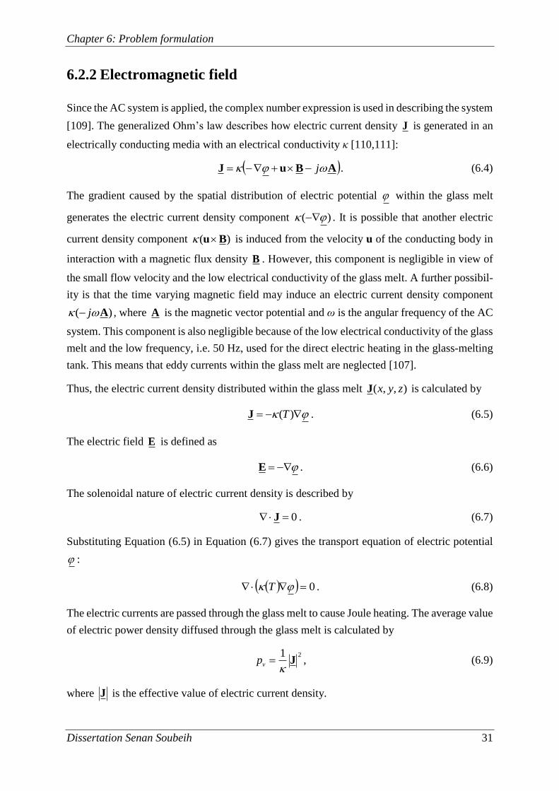
Chapter 6: Problem formulation
Dissertation Senan Soubeih 31
6.2.2 Electromagnetic field
Since the AC system is applied, the complex number expression is used in describing the system
[109]. The generalized Ohm’s law describes how electric current density J is generated in an
electrically conducting media with an electrical conductivity κ [110,111]:
ABuJ j . (6.4)
The gradient caused by the spatial distribution of electric potential within the glass melt
generates the electric current density component )( . It is possible that another electric
current density component )( Bu is induced from the velocity u of the conducting body in
interaction with a magnetic flux density B . However, this component is negligible in view of
the small flow velocity and the low electrical conductivity of the glass melt. A further possibil-
ity is that the time varying magnetic field may induce an electric current density component
)( A j , where A is the magnetic vector potential and ω is the angular frequency of the AC
system. This component is also negligible because of the low electrical conductivity of the glass
melt and the low frequency, i.e. 50 Hz, used for the direct electric heating in the glass-melting
tank. This means that eddy currents within the glass melt are neglected [107].
Thus, the electric current density distributed within the glass melt ),,( zyxJ is calculated by
)(TJ . (6.5)
The electric field E is defined as
E . (6.6)
The solenoidal nature of electric current density is described by
0 J . (6.7)
Substituting Equation (6.5) in Equation (6.7) gives the transport equation of electric potential
:
0 T . (6.8)
The electric currents are passed through the glass melt to cause Joule heating. The average value
of electric power density diffused through the glass melt is calculated by
21
J
vp , (6.9)
where J is the effective value of electric current density.
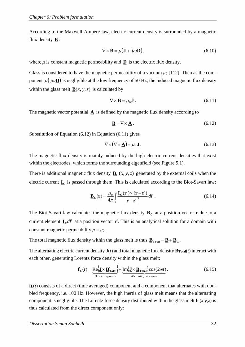
Chapter 6: Problem formulation
Dissertation Senan Soubeih 32
According to the Maxwell-Ampere law, electric current density is surrounded by a magnetic
flux density B :
DJB j , (6.10)
where μ is constant magnetic permeability and D is the electric flux density.
Glass is considered to have the magnetic permeability of a vacuum μ0 [112]. Then as the com-
ponent D j is negligible at the low frequency of 50 Hz, the induced magnetic flux density
within the glass melt ),,( zyxB is calculated by
JB 0 . (6.11)
The magnetic vector potential A is defined by the magnetic flux density according to
AB . (6.12)
Substitution of Equation (6.12) in Equation (6.11) gives
JA 0 . (6.13)
The magnetic flux density is mainly induced by the high electric current densities that exist
within the electrodes, which forms the surrounding eigenfield (see Figure 5.1).
There is additional magnetic flux density ),,( zyxCB generated by the external coils when the
electric current CI is passed through them. This is calculated according to the Biot-Savart law:
l
ld3
0 )()(
4)(
rr
rrrIrB C
C
. (6.14)
The Biot-Savart law calculates the magnetic flux density CB at a position vector r due to a
current element ld CI at a position vector rʹ. This is an analytical solution for a domain with
constant magnetic permeability μ = μ0.
The total magnetic flux density within the glass melt is thus CTotal BBB .
The alternating electric current density J(t) and total magnetic flux density BTotal(t) interact with
each other, generating Lorentz force density within the glass melt:
componentgAlternatincomponentDirect
tt
Total
TotalL BJBJf )2cos(ImRe)(
. (6.15)
fL(t) consists of a direct (time averaged) component and a component that alternates with dou-
bled frequency, i.e. 100 Hz. However, the high inertia of glass melt means that the alternating
component is negligible. The Lorentz force density distributed within the glass melt fL(x,y,z) is
thus calculated from the direct component only:
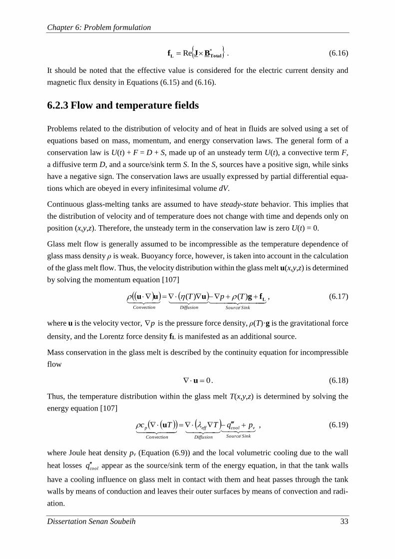
Chapter 6: Problem formulation
Dissertation Senan Soubeih 33
TotalL BJf Re . (6.16)
It should be noted that the effective value is considered for the electric current density and
magnetic flux density in Equations (6.15) and (6.16).
6.2.3 Flow and temperature fields
Problems related to the distribution of velocity and of heat in fluids are solved using a set of
equations based on mass, momentum, and energy conservation laws. The general form of a
conservation law is U(t) + F = D + S, made up of an unsteady term U(t), a convective term F,
a diffusive term D, and a source/sink term S. In the S, sources have a positive sign, while sinks
have a negative sign. The conservation laws are usually expressed by partial differential equa-
tions which are obeyed in every infinitesimal volume dV.
Continuous glass-melting tanks are assumed to have steady-state behavior. This implies that
the distribution of velocity and of temperature does not change with time and depends only on
position (x,y,z). Therefore, the unsteady term in the conservation law is zero U(t) = 0.
Glass melt flow is generally assumed to be incompressible as the temperature dependence of
glass mass density ρ is weak. Buoyancy force, however, is taken into account in the calculation
of the glass melt flow. Thus, the velocity distribution within the glass melt u(x,y,z) is determined
by solving the momentum equation [107]
SinkSourceDiffusionConvection
TpT
/
)()( Lfguuu , (6.17)
where u is the velocity vector, p is the pressure force density, ρ(T)·g is the gravitational force
density, and the Lorentz force density fL is manifested as an additional source.
Mass conservation in the glass melt is described by the continuity equation for incompressible
flow
0 u . (6.18)
Thus, the temperature distribution within the glass melt T(x,y,z) is determined by solving the
energy equation [107]
SinkSource
vcool
Diffusion
eff
Convection
p pqTTc
/
u , (6.19)
where Joule heat density pv (Equation (6.9)) and the local volumetric cooling due to the wall
heat losses coolq appear as the source/sink term of the energy equation, in that the tank walls
have a cooling influence on glass melt in contact with them and heat passes through the tank
walls by means of conduction and leaves their outer surfaces by means of convection and radi-
ation.
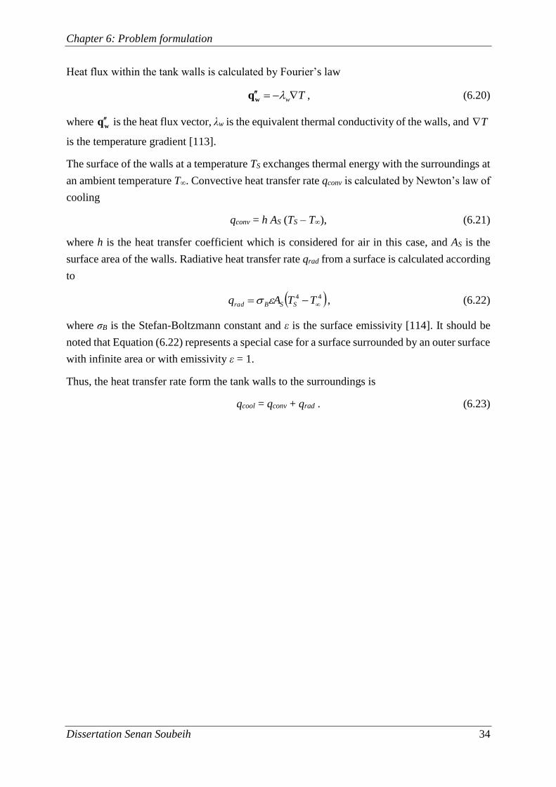
Chapter 6: Problem formulation
Dissertation Senan Soubeih 34
Heat flux within the tank walls is calculated by Fourier’s law
Tw wq , (6.20)
where wq is the heat flux vector, λw is the equivalent thermal conductivity of the walls, and T
is the temperature gradient [113].
The surface of the walls at a temperature TS exchanges thermal energy with the surroundings at
an ambient temperature T∞. Convective heat transfer rate qconv is calculated by Newton’s law of
cooling
qconv = h AS (TS – T∞), (6.21)
where h is the heat transfer coefficient which is considered for air in this case, and AS is the
surface area of the walls. Radiative heat transfer rate qrad from a surface is calculated according
to
44
TTAq SSBrad , (6.22)
where σB is the Stefan-Boltzmann constant and ε is the surface emissivity [114]. It should be
noted that Equation (6.22) represents a special case for a surface surrounded by an outer surface
with infinite area or with emissivity ε = 1.
Thus, the heat transfer rate form the tank walls to the surroundings is
qcool = qconv + qrad . (6.23)
Chapter 7: Numerical methodology
Dissertation Senan Soubeih 35
7 Numerical methodology
Here the subject is the numerical approach employed to couple the calculations, followed by
test-simulations which form part of the model developing process. The test-simulations are per-
formed using simplified examples intended to validate and test the numerical approach.
7.1 Coupling the calculations
Numerically solving the coupled nonlinear system of equations presented in Chapter 6 would
require a simulation tool that is able to calculate coupled electrodynamic, thermodynamic, and
hydrodynamic effects. In modeling the tank, one should also take into account the huge volume
of glass melt (approximately 50 m3) and the complex flow pattern. Numerical simulation of
such a system thus requires a massive computational grid consisting of several million cells.
The computational effort involved in coupling two different simulation tools with an exchange
between electromagnetic field calculation on one side and flow field including temperature field
calculation on the other side would be enormous. Such two-way coupling is necessary as the
value of the temperature-dependent electrical conductivity must be updated in the solution do-
main so that the electric current and Lorentz force densities can be recalculated. Such a highly
complex problem will overload even the available commercial software tools that are suitable
for Multiphysics calculations.
A reliable computational approach must be found that is able to efficiently solve the problem.
The approach taken is to reduce the need for numerical programming and make use of the state
of the art in pre- and post-processing by implementing the electrodynamics calculation in the
commercial software FLUENT. This program was developed to calculate coupled thermody-
namic and hydrodynamic effects on the basis of FVM. Therewith, the governing equations for
the magnetic field are referred to the general form of diffusion equation, making it thus possible
to solve these equations using the same computational algorithm used for flow and temperature
fields, a technique which allows all fields to be calculated iteratively in one computational pro-
cedure. There is a further advantage in using FLUENT: the possibility of calculating the coil
magnetic field by analytical solution using the so-called user-defined function (UDF). It is also
useful that FLUENT has a parallel solver which features solution partitioning using multiple
processes that can be executed on one computer, or on different computers in a network cluster,
which can significantly reduce the computational time [115].
Chapter 7: Numerical methodology
Dissertation Senan Soubeih 36
7.2 Calculating electromagnetic field with FLUENT
FLUENT bases its solution of the partial differential equations of mass, momentum, and energy
conservation on the use of FVM. FLUENT allows the solving of up to 50 user-defined scalar
(UDS) transport equations [116]. For an arbitrary scalar ϕk, FLUENT solves the general scalar
transport equation
Sources
Diffusion
i
kk
Convection
ki
i
Unsteady
k
kS
xu
xt
, Nk ,...,1 . (7.1)
The diffusion coefficient Γk and source term k
S are provided by the user for each of the N
scalar transport equations. The idea is to calculate the electromagnetic field with FLUENT,
which is an innovative use of the program. Then it is possible to calculate the electromagnetic,
the thermodynamic, and the hydrodynamic effects in one computational procedure. Further-
more, the governing equations of the electromagnetic, flow, and temperature fields will thus be
solved using the same kind of computational algorithm [115].
To simplify the discussion initially, what follows is the case of a direct current (DC) system.
As shown in Subsection 6.2.2, electric current density is given by
J , (7.2)
and the solenoidal nature of J is described by
0 J . (7.3)
Substituting Equation (7.2) in Equation (7.3) gives the transport equation of electric potential
φ:
0 . (7.4)
Electric current density induces a magnetic flux density which is given by [110]
JB 0 . (7.5)
The magnetic vector potential A is defined by the magnetic flux density according to
AB . (7.6)
Equation (7.6) substituted in Equation (7.5) gives
JA 0 . (7.7)
Applying the vector equality AAA 2 to the left-hand side of Equation
(7.7), one obtains [117]
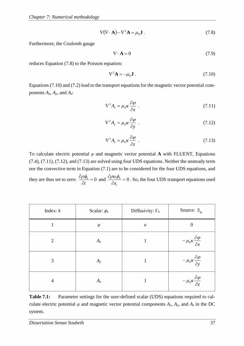
Chapter 7: Numerical methodology
Dissertation Senan Soubeih 37
JAA 0
2 . (7.8)
Furthermore, the Coulomb gauge
0 A (7.9)
reduces Equation (7.8) to the Poisson equation:
JA 0
2 . (7.10)
Equations (7.10) and (7.2) lead to the transport equations for the magnetic vector potential com-
ponents Ax, Ay, and Az:
x
Ax
0
2 . (7.11)
y
Ay
0
2 . (7.12)
z
Az
0
2 . (7.13)
To calculate electric potential φ and magnetic vector potential A with FLUENT, Equations
(7.4), (7.11), (7.12), and (7.13) are solved using four UDS equations. Neither the unsteady term
nor the convective term in Equation (7.1) are to be considered for the four UDS equations, and
they are thus set to zero: 0
t
k and 0
i
ki
x
u . So, the four UDS transport equations used
Index: k Scalar: ϕk Diffusivity: Γk Source: k
S
1 φ κ 0
2 Ax 1 x
0
3 Ay 1 y
0
4 Az 1 z
0
Table 7.1: Parameter settings for the user-defined scalar (UDS) equations required to cal-
culate electric potential φ and magnetic vector potential components Ax, Ay, and Az in the DC
system.
Chapter 7: Numerical methodology
Dissertation Senan Soubeih 38
to calculate φ, Ax, Ay, and Az are defined by setting the parameters for the diffusive and source
terms in Equation (7.1), as shown in Table 7.1.
After that, the calculated values of φ, Ax, Ay, and Az are used to calculate electric current density
J and its induced magnetic flux density B using Equations (7.2) and (7.6) respectively. This is
performed using UDF which can be dynamically loaded with the FLUENT solver.
Also by means of UDF, the additional magnetic flux density generated by the coils BC is cal-
culated using the Biot-Savart law for each turn of each coil:
l
ld3
0 )()(
4)(
rr
rrrIrB C
C
. (7.14)
Equation (7.14) provides an analytical solution for a domain with constant magnetic permea-
bility.
The total magnetic flux density is then defined as
BTotal = B + BC. (7.15)
The Lorentz force density is calculated using UDF for
fL = J × BTotal. (7.16)
fL is set as an additional parameter for source term k
S in the momentum equation which is
solved by FLUENT to calculate the flow field.
Joule heat density caused by J is calculated using UDF for
21
J
vp . (7.17)
Likewise, pv is set as an additional parameter for source term k
S in the energy equation which
is solved by FLUENT to calculate the temperature field.
7.3 Validation by numerical simulation with MAXWELL
In the modeling of a system, validation is evaluating the accuracy of the model by comparing
the results with those from a different modeling approach [118,119]. Numerical models are
usually validated by comparing their results with those of experiments [120]. Another possibil-
ity, when experiments or measurements are not possible, is to compare the results with those
obtained by a different numerical method. This section of the present thesis is largely concerned
with validating the electrodynamics calculation modeled within FLUENT. The FLUENT re-
sults are compared with that of a reference code which employs a different numerical method
for the calculation of the electromagnetic field. The choice of reference software is MAX-
WELL, which was developed to calculate electromagnetic effects on the basis of the Finite
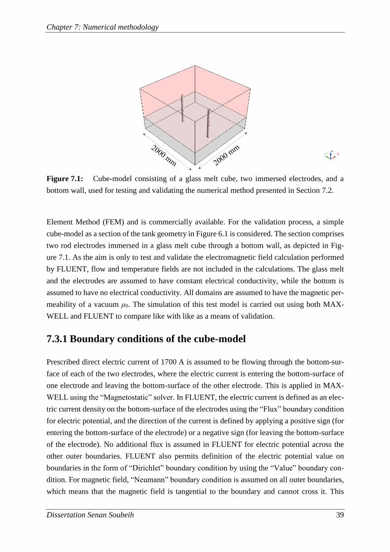
Chapter 7: Numerical methodology
Dissertation Senan Soubeih 39
Element Method (FEM) and is commercially available. For the validation process, a simple
cube-model as a section of the tank geometry in Figure 6.1 is considered. The section comprises
two rod electrodes immersed in a glass melt cube through a bottom wall, as depicted in Fig-
ure 7.1. As the aim is only to test and validate the electromagnetic field calculation performed
by FLUENT, flow and temperature fields are not included in the calculations. The glass melt
and the electrodes are assumed to have constant electrical conductivity, while the bottom is
assumed to have no electrical conductivity. All domains are assumed to have the magnetic per-
meability of a vacuum μ0. The simulation of this test model is carried out using both MAX-
WELL and FLUENT to compare like with like as a means of validation.
7.3.1 Boundary conditions of the cube-model
Prescribed direct electric current of 1700 A is assumed to be flowing through the bottom-sur-
face of each of the two electrodes, where the electric current is entering the bottom-surface of
one electrode and leaving the bottom-surface of the other electrode. This is applied in MAX-
WELL using the “Magnetostatic” solver. In FLUENT, the electric current is defined as an elec-
tric current density on the bottom-surface of the electrodes using the “Flux” boundary condition
for electric potential, and the direction of the current is defined by applying a positive sign (for
entering the bottom-surface of the electrode) or a negative sign (for leaving the bottom-surface
of the electrode). No additional flux is assumed in FLUENT for electric potential across the
other outer boundaries. FLUENT also permits definition of the electric potential value on
boundaries in the form of “Dirichlet” boundary condition by using the “Value” boundary con-
dition. For magnetic field, “Neumann” boundary condition is assumed on all outer boundaries,
which means that the magnetic field is tangential to the boundary and cannot cross it. This
Figure 7.1: Cube-model consisting of a glass melt cube, two immersed electrodes, and a
bottom wall, used for testing and validating the numerical method presented in Section 7.2.
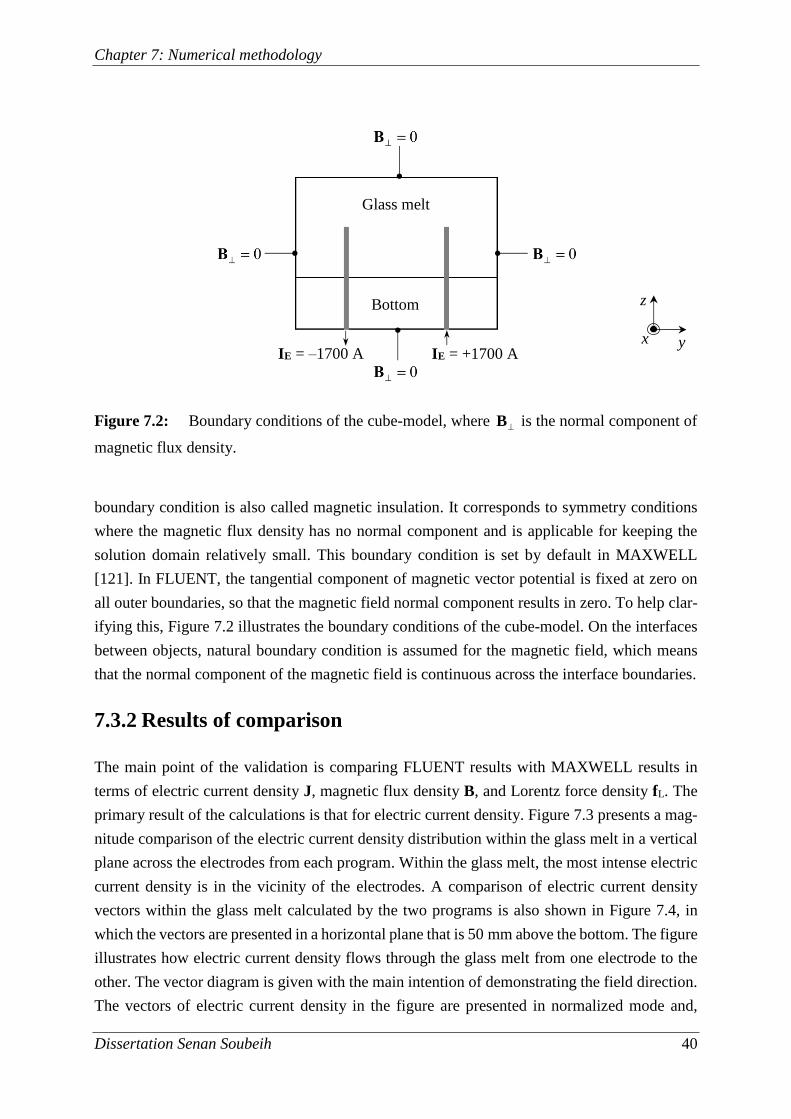
Chapter 7: Numerical methodology
Dissertation Senan Soubeih 40
boundary condition is also called magnetic insulation. It corresponds to symmetry conditions
where the magnetic flux density has no normal component and is applicable for keeping the
solution domain relatively small. This boundary condition is set by default in MAXWELL
[121]. In FLUENT, the tangential component of magnetic vector potential is fixed at zero on
all outer boundaries, so that the magnetic field normal component results in zero. To help clar-
ifying this, Figure 7.2 illustrates the boundary conditions of the cube-model. On the interfaces
between objects, natural boundary condition is assumed for the magnetic field, which means
that the normal component of the magnetic field is continuous across the interface boundaries.
7.3.2 Results of comparison
The main point of the validation is comparing FLUENT results with MAXWELL results in
terms of electric current density J, magnetic flux density B, and Lorentz force density fL. The
primary result of the calculations is that for electric current density. Figure 7.3 presents a mag-
nitude comparison of the electric current density distribution within the glass melt in a vertical
plane across the electrodes from each program. Within the glass melt, the most intense electric
current density is in the vicinity of the electrodes. A comparison of electric current density
vectors within the glass melt calculated by the two programs is also shown in Figure 7.4, in
which the vectors are presented in a horizontal plane that is 50 mm above the bottom. The figure
illustrates how electric current density flows through the glass melt from one electrode to the
other. The vector diagram is given with the main intention of demonstrating the field direction.
The vectors of electric current density in the figure are presented in normalized mode and,
Figure 7.2: Boundary conditions of the cube-model, where B is the normal component of
magnetic flux density.
IE = +1700 A IE = –1700 A
Glass melt
Bottom
y
z
x
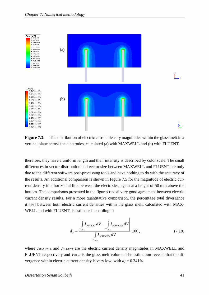
Chapter 7: Numerical methodology
Dissertation Senan Soubeih 41
therefore, they have a uniform length and their intensity is described by color scale. The small
differences in vector distribution and vector size between MAXWELL and FLUENT are only
due to the different software post-processing tools and have nothing to do with the accuracy of
the results. An additional comparison is shown in Figure 7.5 for the magnitude of electric cur-
rent density in a horizontal line between the electrodes, again at a height of 50 mm above the
bottom. The comparisons presented in the figures reveal very good agreement between electric
current density results. For a more quantitative comparison, the percentage total divergence
dJ [%] between both electric current densities within the glass melt, calculated with MAX-
WELL and with FLUENT, is estimated according to
100
Glass
GlassGlass
V
MAXWELL
V
MAXWELL
V
FLUENT
JdVJ
dVJdVJ
d , (7.18)
where JMAXWELL and JFLUENT are the electric current density magnitudes in MAXWELL and
FLUENT respectively and VGlass is the glass melt volume. The estimation reveals that the di-
vergence within electric current density is very low, with dJ = 0.341%.
Figure 7.3: The distribution of electric current density magnitudes within the glass melt in a
vertical plane across the electrodes, calculated (a) with MAXWELL and (b) with FLUENT.
(b)
(a)
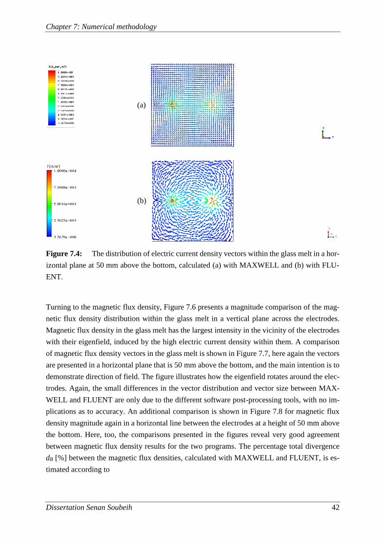
Chapter 7: Numerical methodology
Dissertation Senan Soubeih 42
Turning to the magnetic flux density, Figure 7.6 presents a magnitude comparison of the mag-
netic flux density distribution within the glass melt in a vertical plane across the electrodes.
Magnetic flux density in the glass melt has the largest intensity in the vicinity of the electrodes
with their eigenfield, induced by the high electric current density within them. A comparison
of magnetic flux density vectors in the glass melt is shown in Figure 7.7, here again the vectors
are presented in a horizontal plane that is 50 mm above the bottom, and the main intention is to
demonstrate direction of field. The figure illustrates how the eigenfield rotates around the elec-
trodes. Again, the small differences in the vector distribution and vector size between MAX-
WELL and FLUENT are only due to the different software post-processing tools, with no im-
plications as to accuracy. An additional comparison is shown in Figure 7.8 for magnetic flux
density magnitude again in a horizontal line between the electrodes at a height of 50 mm above
the bottom. Here, too, the comparisons presented in the figures reveal very good agreement
between magnetic flux density results for the two programs. The percentage total divergence
dB [%] between the magnetic flux densities, calculated with MAXWELL and FLUENT, is es-
timated according to
Figure 7.4: The distribution of electric current density vectors within the glass melt in a hor-
izontal plane at 50 mm above the bottom, calculated (a) with MAXWELL and (b) with FLU-
ENT.
(b)
(a)
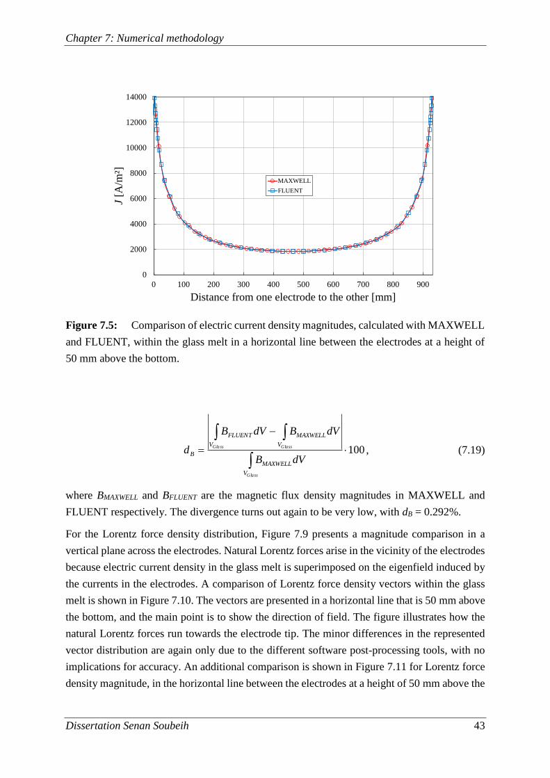
Chapter 7: Numerical methodology
Dissertation Senan Soubeih 43
100
Glass
GlassGlass
V
MAXWELL
V
MAXWELL
V
FLUENT
BdVB
dVBdVB
d , (7.19)
where BMAXWELL and BFLUENT are the magnetic flux density magnitudes in MAXWELL and
FLUENT respectively. The divergence turns out again to be very low, with dB = 0.292%.
For the Lorentz force density distribution, Figure 7.9 presents a magnitude comparison in a
vertical plane across the electrodes. Natural Lorentz forces arise in the vicinity of the electrodes
because electric current density in the glass melt is superimposed on the eigenfield induced by
the currents in the electrodes. A comparison of Lorentz force density vectors within the glass
melt is shown in Figure 7.10. The vectors are presented in a horizontal line that is 50 mm above
the bottom, and the main point is to show the direction of field. The figure illustrates how the
natural Lorentz forces run towards the electrode tip. The minor differences in the represented
vector distribution are again only due to the different software post-processing tools, with no
implications for accuracy. An additional comparison is shown in Figure 7.11 for Lorentz force
density magnitude, in the horizontal line between the electrodes at a height of 50 mm above the
Figure 7.5: Comparison of electric current density magnitudes, calculated with MAXWELL
and FLUENT, within the glass melt in a horizontal line between the electrodes at a height of
50 mm above the bottom.
0
2000
4000
6000
8000
10000
12000
14000
0 100 200 300 400 500 600 700 800 900
J[A
/m²]
Distance from one electrode to the other [mm]
MAXWELL
FLUENT
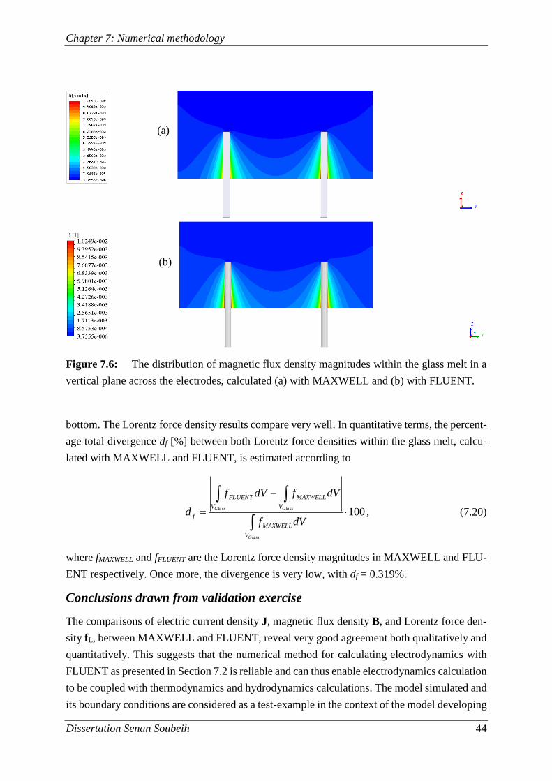
Chapter 7: Numerical methodology
Dissertation Senan Soubeih 44
bottom. The Lorentz force density results compare very well. In quantitative terms, the percent-
age total divergence df [%] between both Lorentz force densities within the glass melt, calcu-
lated with MAXWELL and FLUENT, is estimated according to
100
Glass
GlassGlass
V
MAXWELL
V
MAXWELL
V
FLUENT
fdVf
dVfdVf
d , (7.20)
where fMAXWELL and fFLUENT are the Lorentz force density magnitudes in MAXWELL and FLU-
ENT respectively. Once more, the divergence is very low, with df = 0.319%.
Conclusions drawn from validation exercise
The comparisons of electric current density J, magnetic flux density B, and Lorentz force den-
sity fL, between MAXWELL and FLUENT, reveal very good agreement both qualitatively and
quantitatively. This suggests that the numerical method for calculating electrodynamics with
FLUENT as presented in Section 7.2 is reliable and can thus enable electrodynamics calculation
to be coupled with thermodynamics and hydrodynamics calculations. The model simulated and
its boundary conditions are considered as a test-example in the context of the model developing
Figure 7.6: The distribution of magnetic flux density magnitudes within the glass melt in a
vertical plane across the electrodes, calculated (a) with MAXWELL and (b) with FLUENT.
(b)
(a)
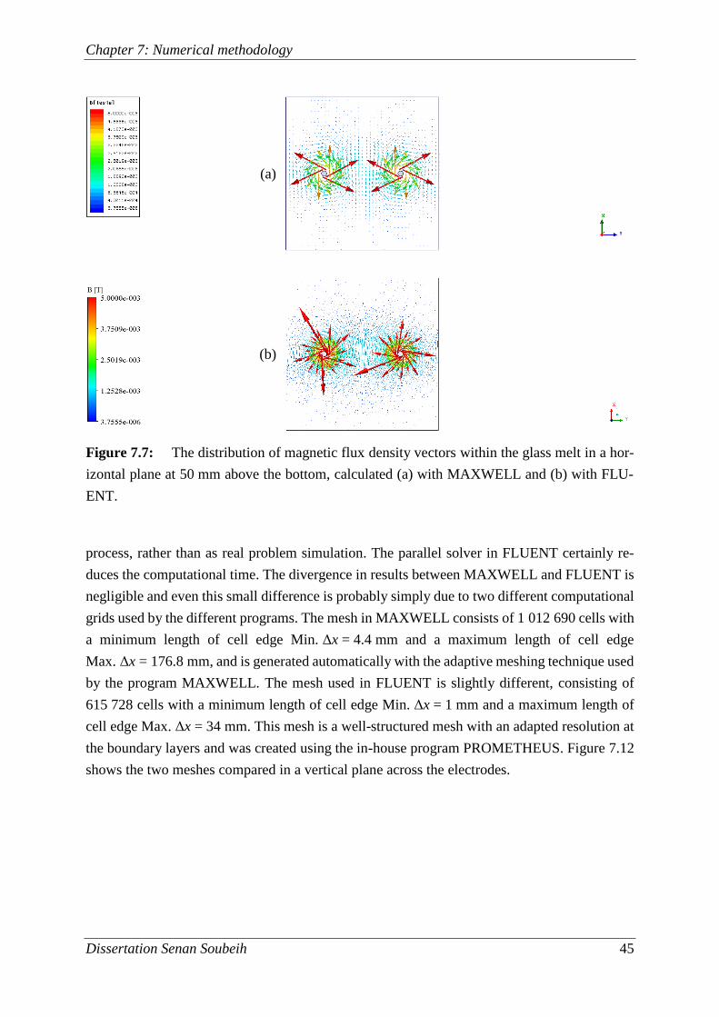
Chapter 7: Numerical methodology
Dissertation Senan Soubeih 45
process, rather than as real problem simulation. The parallel solver in FLUENT certainly re-
duces the computational time. The divergence in results between MAXWELL and FLUENT is
negligible and even this small difference is probably simply due to two different computational
grids used by the different programs. The mesh in MAXWELL consists of 1 012 690 cells with
a minimum length of cell edge Min. Δx = 4.4 mm and a maximum length of cell edge
Max. Δx = 176.8 mm, and is generated automatically with the adaptive meshing technique used
by the program MAXWELL. The mesh used in FLUENT is slightly different, consisting of
615 728 cells with a minimum length of cell edge Min. Δx = 1 mm and a maximum length of
cell edge Max. Δx = 34 mm. This mesh is a well-structured mesh with an adapted resolution at
the boundary layers and was created using the in-house program PROMETHEUS. Figure 7.12
shows the two meshes compared in a vertical plane across the electrodes.
Figure 7.7: The distribution of magnetic flux density vectors within the glass melt in a hor-
izontal plane at 50 mm above the bottom, calculated (a) with MAXWELL and (b) with FLU-
ENT.
(b)
(a)
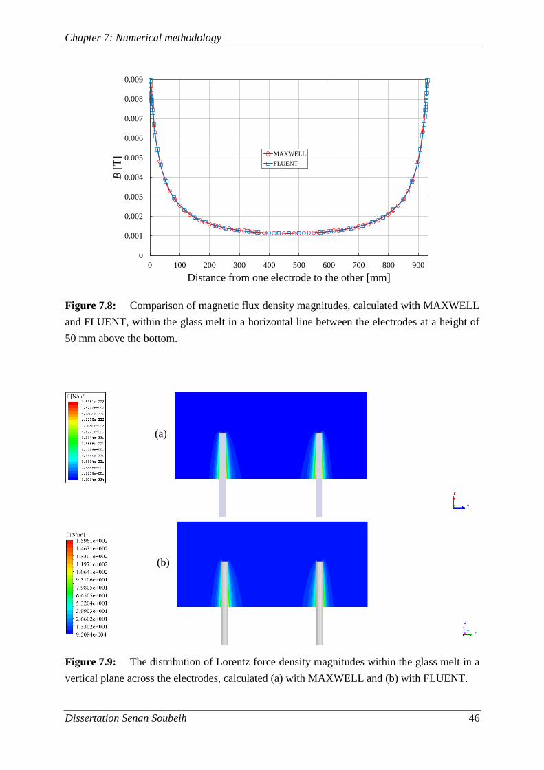
Chapter 7: Numerical methodology
Dissertation Senan Soubeih 46
Figure 7.8: Comparison of magnetic flux density magnitudes, calculated with MAXWELL
and FLUENT, within the glass melt in a horizontal line between the electrodes at a height of
50 mm above the bottom.
Figure 7.9: The distribution of Lorentz force density magnitudes within the glass melt in a
vertical plane across the electrodes, calculated (a) with MAXWELL and (b) with FLUENT.
0
0.001
0.002
0.003
0.004
0.005
0.006
0.007
0.008
0.009
0 100 200 300 400 500 600 700 800 900
B[T
]
Distance from one electrode to the other [mm]
MAXWELL
FLUENT
(b)
(a)
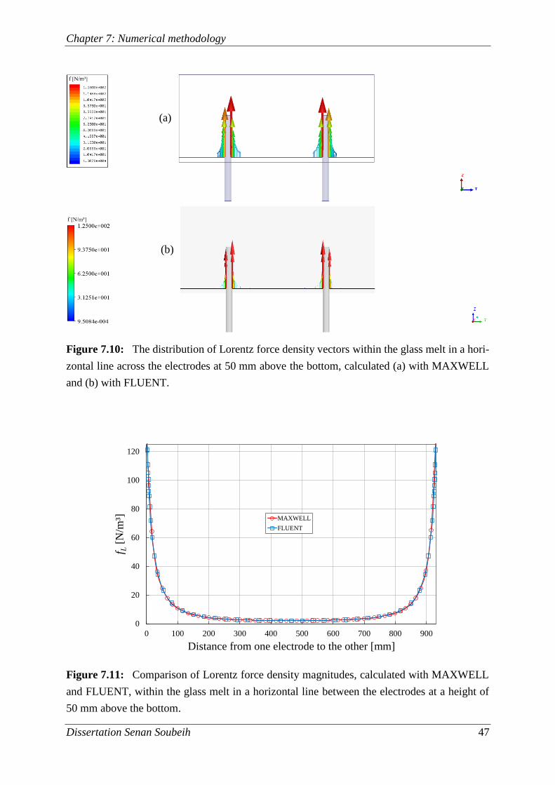
Chapter 7: Numerical methodology
Dissertation Senan Soubeih 47
Figure 7.10: The distribution of Lorentz force density vectors within the glass melt in a hori-
zontal line across the electrodes at 50 mm above the bottom, calculated (a) with MAXWELL
and (b) with FLUENT.
Figure 7.11: Comparison of Lorentz force density magnitudes, calculated with MAXWELL
and FLUENT, within the glass melt in a horizontal line between the electrodes at a height of
50 mm above the bottom.
0
20
40
60
80
100
120
0 100 200 300 400 500 600 700 800 900
f L[N
/m³]
Distance from one electrode to the other [mm]
MAXWELL
FLUENT
(b)
(a)
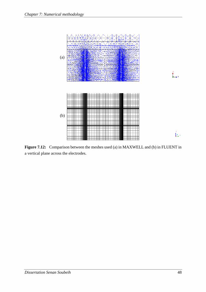
Chapter 7: Numerical methodology
Dissertation Senan Soubeih 48
Figure 7.12: Comparison between the meshes used (a) in MAXWELL and (b) in FLUENT in
a vertical plane across the electrodes.
(b)
(a)
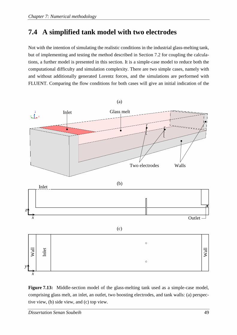
Chapter 7: Numerical methodology
Dissertation Senan Soubeih 49
7.4 A simplified tank model with two electrodes
Not with the intention of simulating the realistic conditions in the industrial glass-melting tank,
but of implementing and testing the method described in Section 7.2 for coupling the calcula-
tions, a further model is presented in this section. It is a simple-case model to reduce both the
computational difficulty and simulation complexity. There are two simple cases, namely with
and without additionally generated Lorentz forces, and the simulations are performed with
FLUENT. Comparing the flow conditions for both cases will give an initial indication of the
Figure 7.13: Middle-section model of the glass-melting tank used as a simple-case model,
comprising glass melt, an inlet, an outlet, two boosting electrodes, and tank walls: (a) perspec-
tive view, (b) side view, and (c) top view.
Inlet
Inle
t
Outlet
Wal
l
Wal
l
Two electrodes
Inlet Glass melt
(a)
(b)
(c)
Walls
x
z
x
y
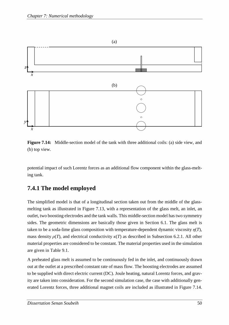
Chapter 7: Numerical methodology
Dissertation Senan Soubeih 50
potential impact of such Lorentz forces as an additional flow component within the glass-melt-
ing tank.
7.4.1 The model employed
The simplified model is that of a longitudinal section taken out from the middle of the glass-
melting tank as illustrated in Figure 7.13, with a representation of the glass melt, an inlet, an
outlet, two boosting electrodes and the tank walls. This middle-section model has two symmetry
sides. The geometric dimensions are basically those given in Section 6.1. The glass melt is
taken to be a soda-lime glass composition with temperature-dependent dynamic viscosity η(T),
mass density ρ(T), and electrical conductivity κ(T) as described in Subsection 6.2.1. All other
material properties are considered to be constant. The material properties used in the simulation
are given in Table 9.1.
A preheated glass melt is assumed to be continuously fed in the inlet, and continuously drawn
out at the outlet at a prescribed constant rate of mass flow. The boosting electrodes are assumed
to be supplied with direct electric current (DC). Joule heating, natural Lorentz forces, and grav-
ity are taken into consideration. For the second simulation case, the case with additionally gen-
erated Lorentz forces, three additional magnet coils are included as illustrated in Figure 7.14.
Figure 7.14: Middle-section model of the tank with three additional coils: (a) side view, and
(b) top view.
(a)
(b)
x
z
x
y
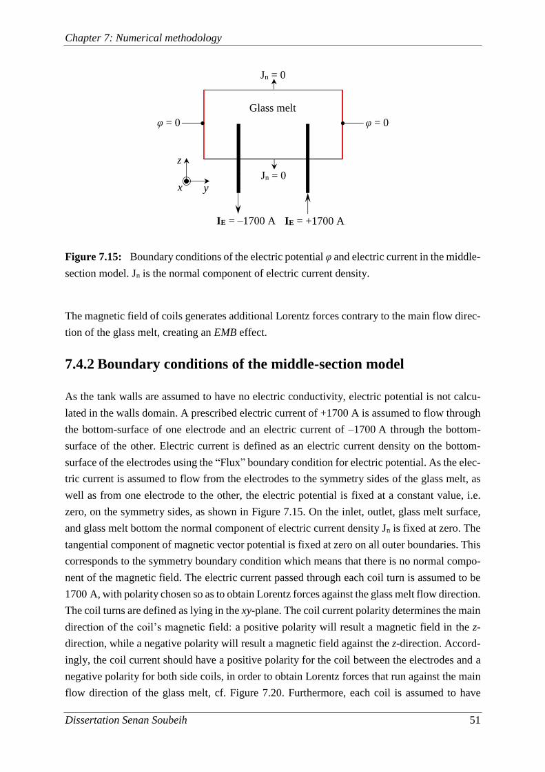
Chapter 7: Numerical methodology
Dissertation Senan Soubeih 51
The magnetic field of coils generates additional Lorentz forces contrary to the main flow direc-
tion of the glass melt, creating an EMB effect.
7.4.2 Boundary conditions of the middle-section model
As the tank walls are assumed to have no electric conductivity, electric potential is not calcu-
lated in the walls domain. A prescribed electric current of +1700 A is assumed to flow through
the bottom-surface of one electrode and an electric current of –1700 A through the bottom-
surface of the other. Electric current is defined as an electric current density on the bottom-
surface of the electrodes using the “Flux” boundary condition for electric potential. As the elec-
tric current is assumed to flow from the electrodes to the symmetry sides of the glass melt, as
well as from one electrode to the other, the electric potential is fixed at a constant value, i.e.
zero, on the symmetry sides, as shown in Figure 7.15. On the inlet, outlet, glass melt surface,
and glass melt bottom the normal component of electric current density Jn is fixed at zero. The
tangential component of magnetic vector potential is fixed at zero on all outer boundaries. This
corresponds to the symmetry boundary condition which means that there is no normal compo-
nent of the magnetic field. The electric current passed through each coil turn is assumed to be
1700 A, with polarity chosen so as to obtain Lorentz forces against the glass melt flow direction.
The coil turns are defined as lying in the xy-plane. The coil current polarity determines the main
direction of the coil’s magnetic field: a positive polarity will result a magnetic field in the z-
direction, while a negative polarity will result a magnetic field against the z-direction. Accord-
ingly, the coil current should have a positive polarity for the coil between the electrodes and a
negative polarity for both side coils, in order to obtain Lorentz forces that run against the main
flow direction of the glass melt, cf. Figure 7.20. Furthermore, each coil is assumed to have
Figure 7.15: Boundary conditions of the electric potential φ and electric current in the middle-
section model. Jn is the normal component of electric current density.
y
z
x
IE = +1700 A IE = –1700 A
φ = 0 φ = 0
Glass melt
Jn = 0
Jn = 0
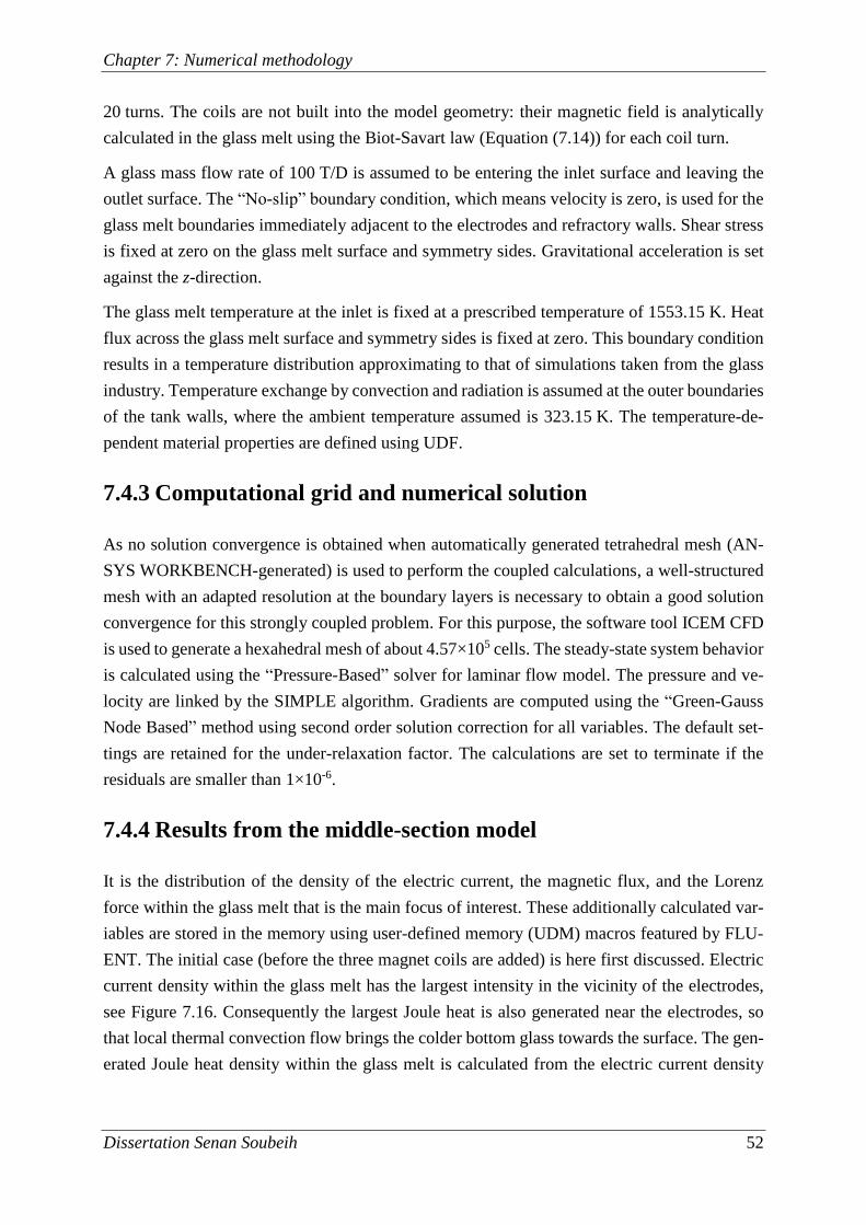
Chapter 7: Numerical methodology
Dissertation Senan Soubeih 52
20 turns. The coils are not built into the model geometry: their magnetic field is analytically
calculated in the glass melt using the Biot-Savart law (Equation (7.14)) for each coil turn.
A glass mass flow rate of 100 T/D is assumed to be entering the inlet surface and leaving the
outlet surface. The “No-slip” boundary condition, which means velocity is zero, is used for the
glass melt boundaries immediately adjacent to the electrodes and refractory walls. Shear stress
is fixed at zero on the glass melt surface and symmetry sides. Gravitational acceleration is set
against the z-direction.
The glass melt temperature at the inlet is fixed at a prescribed temperature of 1553.15 K. Heat
flux across the glass melt surface and symmetry sides is fixed at zero. This boundary condition
results in a temperature distribution approximating to that of simulations taken from the glass
industry. Temperature exchange by convection and radiation is assumed at the outer boundaries
of the tank walls, where the ambient temperature assumed is 323.15 K. The temperature-de-
pendent material properties are defined using UDF.
7.4.3 Computational grid and numerical solution
As no solution convergence is obtained when automatically generated tetrahedral mesh (AN-
SYS WORKBENCH-generated) is used to perform the coupled calculations, a well-structured
mesh with an adapted resolution at the boundary layers is necessary to obtain a good solution
convergence for this strongly coupled problem. For this purpose, the software tool ICEM CFD
is used to generate a hexahedral mesh of about 4.57×10⁵ cells. The steady-state system behavior
is calculated using the “Pressure-Based” solver for laminar flow model. The pressure and ve-
locity are linked by the SIMPLE algorithm. Gradients are computed using the “Green-Gauss
Node Based” method using second order solution correction for all variables. The default set-
tings are retained for the under-relaxation factor. The calculations are set to terminate if the
residuals are smaller than 1×10⁻⁶.
7.4.4 Results from the middle-section model
It is the distribution of the density of the electric current, the magnetic flux, and the Lorenz
force within the glass melt that is the main focus of interest. These additionally calculated var-
iables are stored in the memory using user-defined memory (UDM) macros featured by FLU-
ENT. The initial case (before the three magnet coils are added) is here first discussed. Electric
current density within the glass melt has the largest intensity in the vicinity of the electrodes,
see Figure 7.16. Consequently the largest Joule heat is also generated near the electrodes, so
that local thermal convection flow brings the colder bottom glass towards the surface. The gen-
erated Joule heat density within the glass melt is calculated from the electric current density
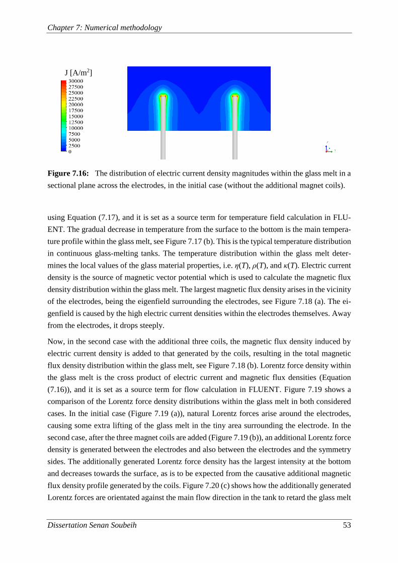
Chapter 7: Numerical methodology
Dissertation Senan Soubeih 53
using Equation (7.17), and it is set as a source term for temperature field calculation in FLU-
ENT. The gradual decrease in temperature from the surface to the bottom is the main tempera-
ture profile within the glass melt, see Figure 7.17 (b). This is the typical temperature distribution
in continuous glass-melting tanks. The temperature distribution within the glass melt deter-
mines the local values of the glass material properties, i.e. η(T), ρ(T), and κ(T). Electric current
density is the source of magnetic vector potential which is used to calculate the magnetic flux
density distribution within the glass melt. The largest magnetic flux density arises in the vicinity
of the electrodes, being the eigenfield surrounding the electrodes, see Figure 7.18 (a). The ei-
genfield is caused by the high electric current densities within the electrodes themselves. Away
from the electrodes, it drops steeply.
Now, in the second case with the additional three coils, the magnetic flux density induced by
electric current density is added to that generated by the coils, resulting in the total magnetic
flux density distribution within the glass melt, see Figure 7.18 (b). Lorentz force density within
the glass melt is the cross product of electric current and magnetic flux densities (Equation
(7.16)), and it is set as a source term for flow calculation in FLUENT. Figure 7.19 shows a
comparison of the Lorentz force density distributions within the glass melt in both considered
cases. In the initial case (Figure 7.19 (a)), natural Lorentz forces arise around the electrodes,
causing some extra lifting of the glass melt in the tiny area surrounding the electrode. In the
second case, after the three magnet coils are added (Figure 7.19 (b)), an additional Lorentz force
density is generated between the electrodes and also between the electrodes and the symmetry
sides. The additionally generated Lorentz force density has the largest intensity at the bottom
and decreases towards the surface, as is to be expected from the causative additional magnetic
flux density profile generated by the coils. Figure 7.20 (c) shows how the additionally generated
Lorentz forces are orientated against the main flow direction in the tank to retard the glass melt
Figure 7.16: The distribution of electric current density magnitudes within the glass melt in a
sectional plane across the electrodes, in the initial case (without the additional magnet coils).
J [A/m2]
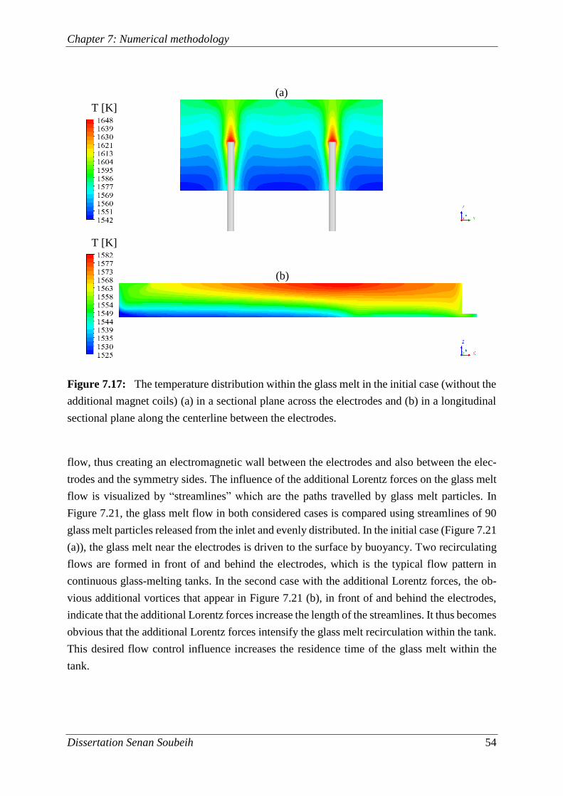
Chapter 7: Numerical methodology
Dissertation Senan Soubeih 54
flow, thus creating an electromagnetic wall between the electrodes and also between the elec-
trodes and the symmetry sides. The influence of the additional Lorentz forces on the glass melt
flow is visualized by “streamlines” which are the paths travelled by glass melt particles. In
Figure 7.21, the glass melt flow in both considered cases is compared using streamlines of 90
glass melt particles released from the inlet and evenly distributed. In the initial case (Figure 7.21
(a)), the glass melt near the electrodes is driven to the surface by buoyancy. Two recirculating
flows are formed in front of and behind the electrodes, which is the typical flow pattern in
continuous glass-melting tanks. In the second case with the additional Lorentz forces, the ob-
vious additional vortices that appear in Figure 7.21 (b), in front of and behind the electrodes,
indicate that the additional Lorentz forces increase the length of the streamlines. It thus becomes
obvious that the additional Lorentz forces intensify the glass melt recirculation within the tank.
This desired flow control influence increases the residence time of the glass melt within the
tank.
Figure 7.17: The temperature distribution within the glass melt in the initial case (without the
additional magnet coils) (a) in a sectional plane across the electrodes and (b) in a longitudinal
sectional plane along the centerline between the electrodes.
T [K]
(b)
(a)
T [K]
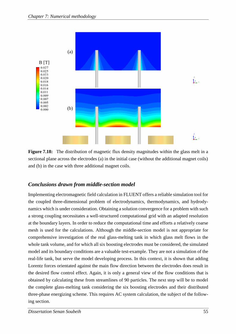
Chapter 7: Numerical methodology
Dissertation Senan Soubeih 55
Conclusions drawn from middle-section model
Implementing electromagnetic field calculation in FLUENT offers a reliable simulation tool for
the coupled three-dimensional problem of electrodynamics, thermodynamics, and hydrody-
namics which is under consideration. Obtaining a solution convergence for a problem with such
a strong coupling necessitates a well-structured computational grid with an adapted resolution
at the boundary layers. In order to reduce the computational time and efforts a relatively coarse
mesh is used for the calculations. Although the middle-section model is not appropriate for
comprehensive investigation of the real glass-melting tank in which glass melt flows in the
whole tank volume, and for which all six boosting electrodes must be considered, the simulated
model and its boundary conditions are a valuable test-example. They are not a simulation of the
real-life tank, but serve the model developing process. In this context, it is shown that adding
Lorentz forces orientated against the main flow direction between the electrodes does result in
the desired flow control effect. Again, it is only a general view of the flow conditions that is
obtained by calculating these from streamlines of 90 particles. The next step will be to model
the complete glass-melting tank considering the six boosting electrodes and their distributed
three-phase energizing scheme. This requires AC system calculation, the subject of the follow-
ing section.
Figure 7.18: The distribution of magnetic flux density magnitudes within the glass melt in a
sectional plane across the electrodes (a) in the initial case (without the additional magnet coils)
and (b) in the case with three additional magnet coils.
B [T]
(b)
(a)
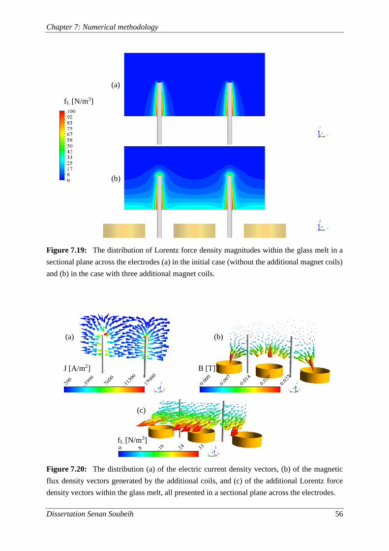
Chapter 7: Numerical methodology
Dissertation Senan Soubeih 56
Figure 7.19: The distribution of Lorentz force density magnitudes within the glass melt in a
sectional plane across the electrodes (a) in the initial case (without the additional magnet coils)
and (b) in the case with three additional magnet coils.
Figure 7.20: The distribution (a) of the electric current density vectors, (b) of the magnetic
flux density vectors generated by the additional coils, and (c) of the additional Lorentz force
density vectors within the glass melt, all presented in a sectional plane across the electrodes.
fL [N/m3]
(b)
(a)
(b)
(c)
(a)
fL [N/m3]
B [T] J [A/m2]
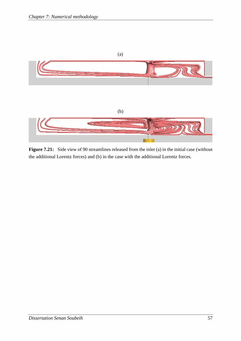
Chapter 7: Numerical methodology
Dissertation Senan Soubeih 57
Figure 7.21: Side view of 90 streamlines released from the inlet (a) in the initial case (without
the additional Lorentz forces) and (b) in the case with the additional Lorentz forces.
(a)
(b)
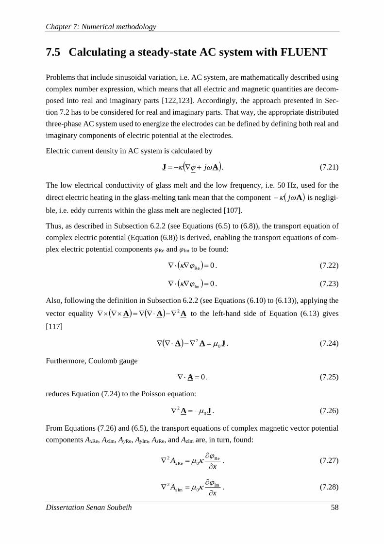
Chapter 7: Numerical methodology
Dissertation Senan Soubeih 58
7.5 Calculating a steady-state AC system with FLUENT
Problems that include sinusoidal variation, i.e. AC system, are mathematically described using
complex number expression, which means that all electric and magnetic quantities are decom-
posed into real and imaginary parts [122,123]. Accordingly, the approach presented in Sec-
tion 7.2 has to be considered for real and imaginary parts. That way, the appropriate distributed
three-phase AC system used to energize the electrodes can be defined by defining both real and
imaginary components of electric potential at the electrodes.
Electric current density in AC system is calculated by
AJ j . (7.21)
The low electrical conductivity of glass melt and the low frequency, i.e. 50 Hz, used for the
direct electric heating in the glass-melting tank mean that the component A j is negligi-
ble, i.e. eddy currents within the glass melt are neglected [107].
Thus, as described in Subsection 6.2.2 (see Equations (6.5) to (6.8)), the transport equation of
complex electric potential (Equation (6.8)) is derived, enabling the transport equations of com-
plex electric potential components φRe and φIm to be found:
0Re . (7.22)
0Im . (7.23)
Also, following the definition in Subsection 6.2.2 (see Equations (6.10) to (6.13)), applying the
vector equality AAA 2 to the left-hand side of Equation (6.13) gives
[117]
JAA 0
2 . (7.24)
Furthermore, Coulomb gauge
0 A . (7.25)
reduces Equation (7.24) to the Poisson equation:
JA 0
2 . (7.26)
From Equations (7.26) and (6.5), the transport equations of complex magnetic vector potential
components AxRe, AxIm, AyRe, AyIm, AzRe, and AzIm are, in turn, found:
x
Ax
Re
0Re
2 . (7.27)
x
Ax
Im
0Im
2 . (7.28)
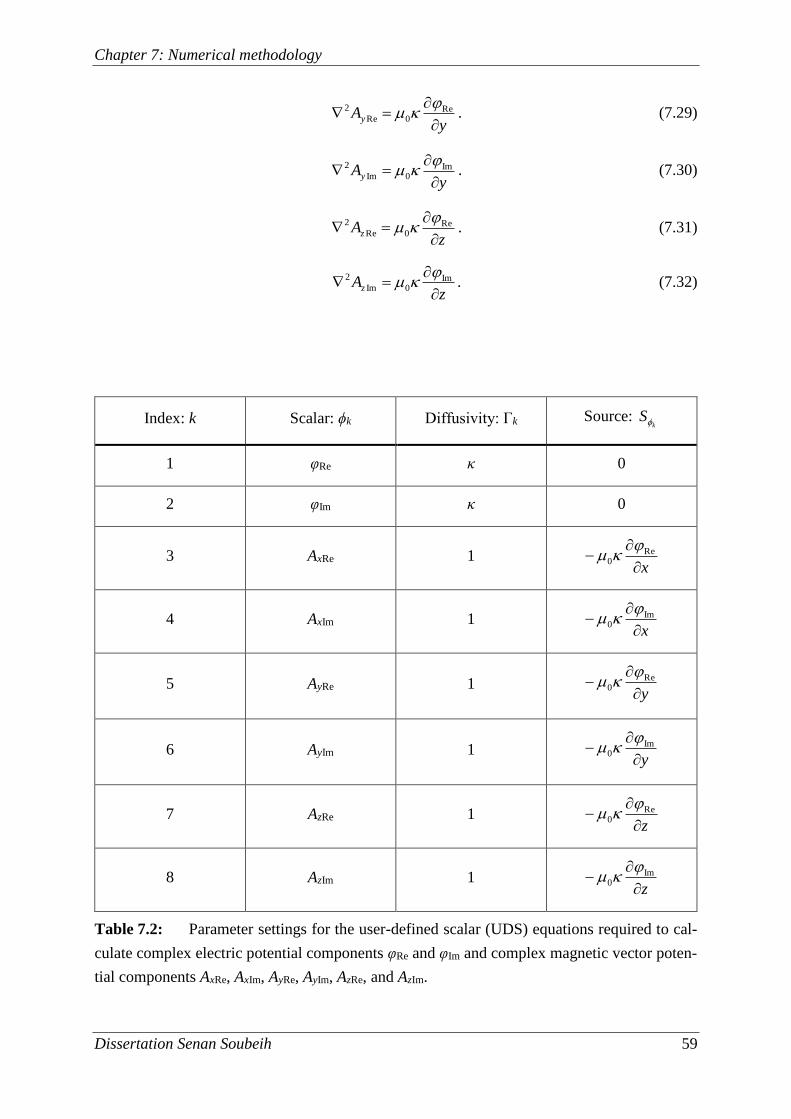
Chapter 7: Numerical methodology
Dissertation Senan Soubeih 59
y
Ay
Re
0Re
2 . (7.29)
y
Ay
Im
0Im
2 . (7.30)
z
Az
Re
0Re
2 . (7.31)
z
Az
Im
0Im
2 . (7.32)
Index: k Scalar: ϕk Diffusivity: Γk Source: k
S
1 φRe κ 0
2 φIm κ 0
3 AxRe 1 x
Re
0
4 AxIm 1 x
Im
0
5 AyRe 1 y
Re
0
6 AyIm 1 y
Im
0
7 AzRe 1 z
Re
0
8 AzIm 1 z
Im
0
Table 7.2: Parameter settings for the user-defined scalar (UDS) equations required to cal-
culate complex electric potential components φRe and φIm and complex magnetic vector poten-
tial components AxRe, AxIm, AyRe, AyIm, AzRe, and AzIm.
Chapter 7: Numerical methodology
Dissertation Senan Soubeih 60
Equations (7.22), (7.23), (7.27), (7.28), (7.29), (7.30), (7.31), and (7.32) are solved using eight
UDS equations, as defined in Table 7.2. Both the unsteady term and the convective term in
Equation (7.1) are set to zero.
After that, the calculated values of φRe, φIm, AxRe, AxIm, AyRe, AyIm, AzRe, and AzIm are used to
calculate electric current density J and its induced magnetic flux density B using Equations
(6.5) and (6.12) respectively. This is performed using UDF which can be dynamically loaded
with the FLUENT solver.
Also by means of UDF, the additional complex magnetic flux density generated by the coils
CB is calculated using the Biot-Savart law for each turn of each coil, i.e. Equation (6.14), which
provides an analytical solution for a domain with constant magnetic permeability.
The total complex magnetic flux density is then defined as
CTotal BBB . (7.33)
Lorentz force density fL (time averaged) is calculated using UDF for Equation (6.16). Further-
more, fL is set as an additional parameter for source term k
S in the momentum equation which
is solved by FLUENT to calculate the flow field.
Joule heat density pv is calculated using UDF for Equation (6.9) and set as an additional param-
eter for source term k
S in the energy equation which is solved by FLUENT to calculate the
temperature field.
Chapter 8: Numerical grid, solution, and accuracy
Dissertation Senan Soubeih 61
8 Numerical grid, solution, and accuracy
This chapter gives details of the computational grid on which the numerical solution is created.
There follows a note on the numerical solution for the governing equations. Finally, various
studies are carried out to verify the numerical accuracy.
8.1 Computational grid
To obtain a numerical solution of partial differential equations, the computational domain re-
quires division into geometrical elements (cells). The resultant cell structure forms the compu-
tational grid (mesh), which can be also viewed as points (nodes) connected by straight lines.
Mesh is one of the most important considerations for numerical simulations as it is the structure
on which the numerical solution is built [124]. The structure is basically of triangles or quadri-
laterals in two-dimensions, and tetrahedra or hexahedra in three-dimensions. As hexahedral
cells provide higher solution accuracy than tetrahedral cells, they tend to be more numerically
stable. Also, when a hexahedral mesh is compared with a tetrahedral one with the same number
of nodes, the number of elements is several times lower. Consequently, hexahedral meshes offer
reduced numerical error and less computational time than tetrahedral ones. On the other hand,
for volume mesh generation, tetrahedral mesh is more easily generated even for models with
complex geometries. Tetrahedral mesh generators also provide more automatic generation pro-
cess with the ability to add mesh controls to improve the accuracy in critical regions. In contrast,
hexahedral mesh generation is more difficult to perform and automate, and takes several orders
of magnitude longer than tetrahedral mesh generation [125].
The mesh quality strongly influences the simulation accuracy. In general, fluid dynamics sim-
ulations require very high-quality meshes in both cell shape and smoothness of size variation.
For the strongly coupled problem of hydrodynamics, thermodynamics, and electrodynamics
considered in this work, the test simulations have shown that no solution convergence can be
obtained using an automatically generated unstructured mesh, i.e. tetrahedral mesh. The use of
a structured mesh, i.e. hexahedral mesh, thus becomes a basic prerequisite for the numerical
simulations. Both geometric configuration and physical solution must be considered in design-
ing the mesh structure. The mesh interior should vary smoothly between the boundaries. As
distribution within the mesh is critical for numerical solution, it should capture the physical
field features. The physical field should be properly resolved in critical regions to minimize the
variation in the field variables from cell to cell. In general, no field passage should be repre-
sented by fewer than five cells and the change in cell size should be gradual. For high-quality
meshes, highly skewed cells and cells with high aspect ratios should be avoided where possible,
as such badly shaped cells tend to decrease the numerical stability. Skewness represents the
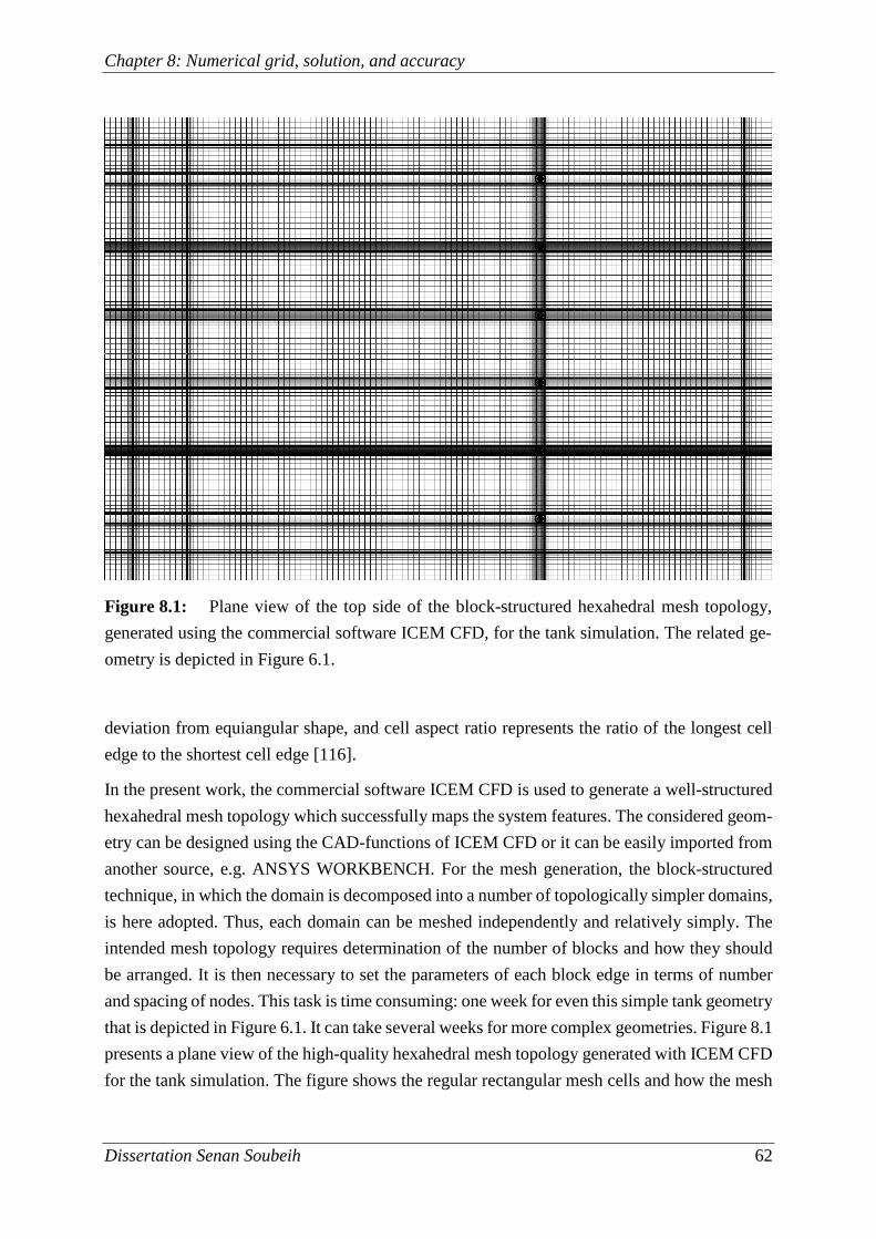
Chapter 8: Numerical grid, solution, and accuracy
Dissertation Senan Soubeih 62
deviation from equiangular shape, and cell aspect ratio represents the ratio of the longest cell
edge to the shortest cell edge [116].
In the present work, the commercial software ICEM CFD is used to generate a well-structured
hexahedral mesh topology which successfully maps the system features. The considered geom-
etry can be designed using the CAD-functions of ICEM CFD or it can be easily imported from
another source, e.g. ANSYS WORKBENCH. For the mesh generation, the block-structured
technique, in which the domain is decomposed into a number of topologically simpler domains,
is here adopted. Thus, each domain can be meshed independently and relatively simply. The
intended mesh topology requires determination of the number of blocks and how they should
be arranged. It is then necessary to set the parameters of each block edge in terms of number
and spacing of nodes. This task is time consuming: one week for even this simple tank geometry
that is depicted in Figure 6.1. It can take several weeks for more complex geometries. Figure 8.1
presents a plane view of the high-quality hexahedral mesh topology generated with ICEM CFD
for the tank simulation. The figure shows the regular rectangular mesh cells and how the mesh
Figure 8.1: Plane view of the top side of the block-structured hexahedral mesh topology,
generated using the commercial software ICEM CFD, for the tank simulation. The related ge-
ometry is depicted in Figure 6.1.
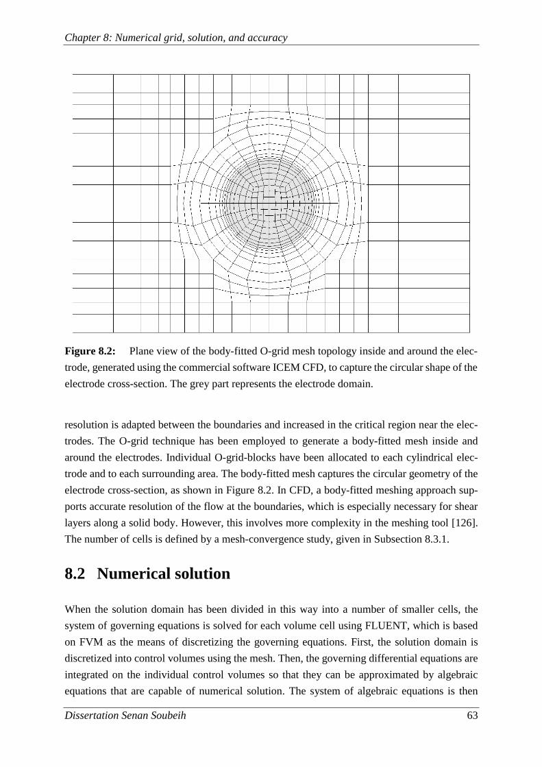
Chapter 8: Numerical grid, solution, and accuracy
Dissertation Senan Soubeih 63
resolution is adapted between the boundaries and increased in the critical region near the elec-
trodes. The O-grid technique has been employed to generate a body-fitted mesh inside and
around the electrodes. Individual O-grid-blocks have been allocated to each cylindrical elec-
trode and to each surrounding area. The body-fitted mesh captures the circular geometry of the
electrode cross-section, as shown in Figure 8.2. In CFD, a body-fitted meshing approach sup-
ports accurate resolution of the flow at the boundaries, which is especially necessary for shear
layers along a solid body. However, this involves more complexity in the meshing tool [126].
The number of cells is defined by a mesh-convergence study, given in Subsection 8.3.1.
8.2 Numerical solution
When the solution domain has been divided in this way into a number of smaller cells, the
system of governing equations is solved for each volume cell using FLUENT, which is based
on FVM as the means of discretizing the governing equations. First, the solution domain is
discretized into control volumes using the mesh. Then, the governing differential equations are
integrated on the individual control volumes so that they can be approximated by algebraic
equations that are capable of numerical solution. The system of algebraic equations is then
Figure 8.2: Plane view of the body-fitted O-grid mesh topology inside and around the elec-
trode, generated using the commercial software ICEM CFD, to capture the circular shape of the
electrode cross-section. The grey part represents the electrode domain.
Chapter 8: Numerical grid, solution, and accuracy
Dissertation Senan Soubeih 64
solved to produce discrete values that approximate the solution of the partial differential system.
The solution loop is carried out iteratively to converge the numerical solution. A steady-state
system behavior is calculated with FLUENT using the Pressure-Based solver which was devel-
oped for low-speed incompressible flows. The laminar flow model is specified in the present
case. Pressure and velocity are linked by the SIMPLE algorithm, which is suitable for compli-
cated problems. Gradients are computed using the Green-Gauss Node Based method, as this
method will give higher accuracy than the cell based one. For all variables, second order solu-
tion correction is the option chosen, to provide the highest accuracy of the convergence. Less
convergence stability is, however, available with this option. To achieve stable convergence
behavior, the under-relaxation factors of density, body force, momentum, energy and all UDS’s
are reduced from their default values to 0.7, 0.9, 0.5, 0.9, and 0.9 respectively. Under-relaxation
of equations is used to control the update of calculated variables at each iteration. Reducing
under-relaxation factors is usually a necessity in strongly coupled problems where unstable
convergence behavior can be observed. The technique damps strong parameter variations, giv-
ing the solution algorithm a certain number of iterations to adjust to the new parameters. Nev-
ertheless, convergence behavior of a completely stable kind is still not achievable. To overcome
this problem, the initial conditions are built up gradually over two hundred iterations. These are
performed using cell based gradient computation and first order solution correction, providing
the greater convergence stability which is desirable regardless of the lower accuracy. It is a
feature of this initial calculation that an initial temperature must be set or there will be calcula-
tion disturbance. The initial guess gained over the two hundred iterations is then used as a start
solution for the simulation. The convergence criterion for terminating the calculation is speci-
fied by a study as described in Subsection 8.3.2. After the steady-state simulation has been
calculated, the velocity vectors will be saved in each grid cell. There will thus be a mapped
velocity in the solution domain. RTD can then be calculated using the particle tracing technique
in CFD. This technique uses an infinitesimal volume of material called a “particle” to follow
the velocity vectors. In this way, particle trajectory and particle residence time are calculated.
The particle trajectory (also called a streamline) is the curve that is tangential to the velocity
vectors. The particle tracing process is available in FLUENT within the “Discrete Phase
Model”.
8.3 Verification and accuracy
Solution verification is the process of evaluating the numerical accuracy of the obtained solu-
tion. As such, it deals with solution accuracy and should not be confused with the validation
term which addresses the modeling accuracy. Both processes are, of course, essential for every
numerical simulation as they are the basis for quantifying the accuracy of the results and the
reliability of the calculation [118,119]. In this section, the focus is on the verification.
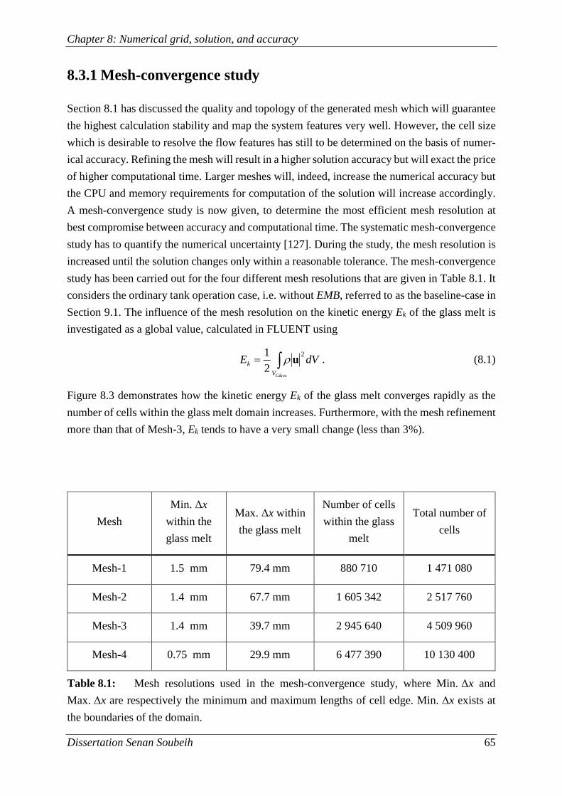
Chapter 8: Numerical grid, solution, and accuracy
Dissertation Senan Soubeih 65
8.3.1 Mesh-convergence study
Section 8.1 has discussed the quality and topology of the generated mesh which will guarantee
the highest calculation stability and map the system features very well. However, the cell size
which is desirable to resolve the flow features has still to be determined on the basis of numer-
ical accuracy. Refining the mesh will result in a higher solution accuracy but will exact the price
of higher computational time. Larger meshes will, indeed, increase the numerical accuracy but
the CPU and memory requirements for computation of the solution will increase accordingly.
A mesh-convergence study is now given, to determine the most efficient mesh resolution at
best compromise between accuracy and computational time. The systematic mesh-convergence
study has to quantify the numerical uncertainty [127]. During the study, the mesh resolution is
increased until the solution changes only within a reasonable tolerance. The mesh-convergence
study has been carried out for the four different mesh resolutions that are given in Table 8.1. It
considers the ordinary tank operation case, i.e. without EMB, referred to as the baseline-case in
Section 9.1. The influence of the mesh resolution on the kinetic energy Ek of the glass melt is
investigated as a global value, calculated in FLUENT using
GlassV
k dVE2
2
1u . (8.1)
Figure 8.3 demonstrates how the kinetic energy Ek of the glass melt converges rapidly as the
number of cells within the glass melt domain increases. Furthermore, with the mesh refinement
more than that of Mesh-3, Ek tends to have a very small change (less than 3%).
Mesh
Min. Δx
within the
glass melt
Max. Δx within
the glass melt
Number of cells
within the glass
melt
Total number of
cells
Mesh-1 1.5 mm 79.4 mm 880 710 1 471 080
Mesh-2 1.4 mm 67.7 mm 1 605 342 2 517 760
Mesh-3 1.4 mm 39.7 mm 2 945 640 4 509 960
Mesh-4 0.75 mm 29.9 mm 6 477 390 10 130 400
Table 8.1: Mesh resolutions used in the mesh-convergence study, where Min. Δx and
Max. Δx are respectively the minimum and maximum lengths of cell edge. Min. Δx exists at
the boundaries of the domain.
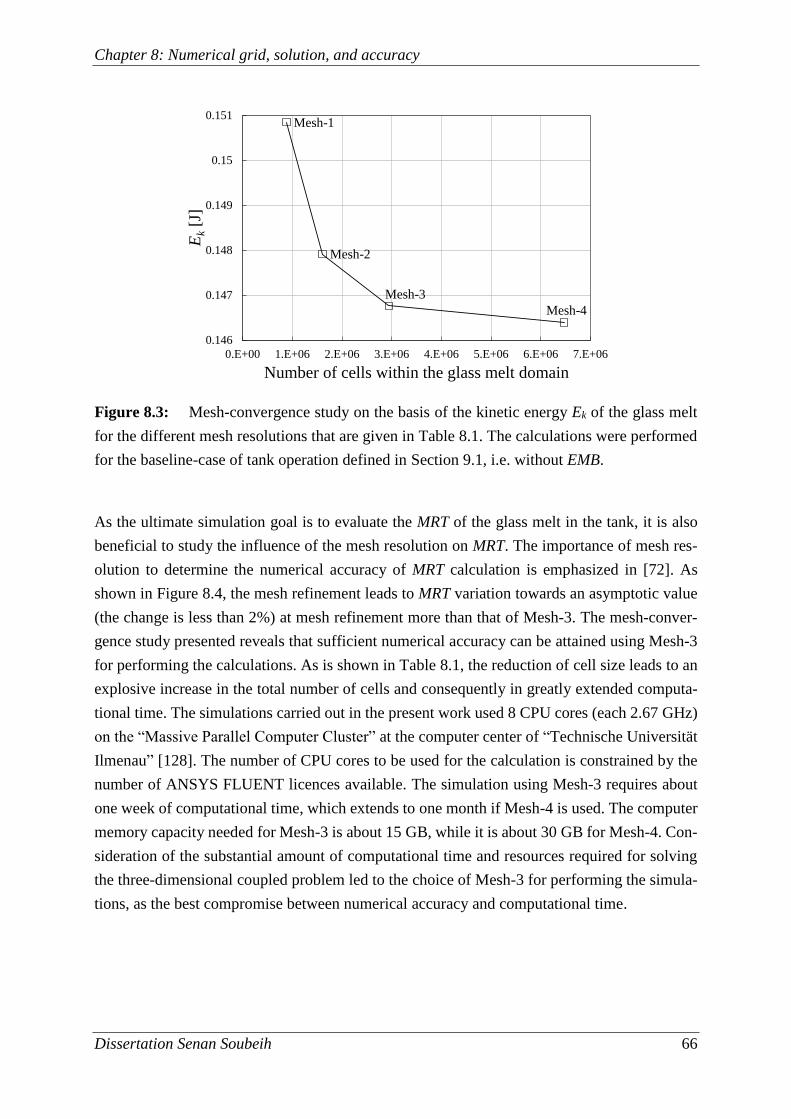
Chapter 8: Numerical grid, solution, and accuracy
Dissertation Senan Soubeih 66
As the ultimate simulation goal is to evaluate the MRT of the glass melt in the tank, it is also
beneficial to study the influence of the mesh resolution on MRT. The importance of mesh res-
olution to determine the numerical accuracy of MRT calculation is emphasized in [72]. As
shown in Figure 8.4, the mesh refinement leads to MRT variation towards an asymptotic value
(the change is less than 2%) at mesh refinement more than that of Mesh-3. The mesh-conver-
gence study presented reveals that sufficient numerical accuracy can be attained using Mesh-3
for performing the calculations. As is shown in Table 8.1, the reduction of cell size leads to an
explosive increase in the total number of cells and consequently in greatly extended computa-
tional time. The simulations carried out in the present work used 8 CPU cores (each 2.67 GHz)
on the “Massive Parallel Computer Cluster” at the computer center of “Technische Universität
Ilmenau” [128]. The number of CPU cores to be used for the calculation is constrained by the
number of ANSYS FLUENT licences available. The simulation using Mesh-3 requires about
one week of computational time, which extends to one month if Mesh-4 is used. The computer
memory capacity needed for Mesh-3 is about 15 GB, while it is about 30 GB for Mesh-4. Con-
sideration of the substantial amount of computational time and resources required for solving
the three-dimensional coupled problem led to the choice of Mesh-3 for performing the simula-
tions, as the best compromise between numerical accuracy and computational time.
Figure 8.3: Mesh-convergence study on the basis of the kinetic energy Ek of the glass melt
for the different mesh resolutions that are given in Table 8.1. The calculations were performed
for the baseline-case of tank operation defined in Section 9.1, i.e. without EMB.
0.146
0.147
0.148
0.149
0.15
0.151
0.E+00 1.E+06 2.E+06 3.E+06 4.E+06 5.E+06 6.E+06 7.E+06
Ek
[J]
Number of cells within the glass melt domain
Mesh-1
Mesh-2
Mesh-3
Mesh-4
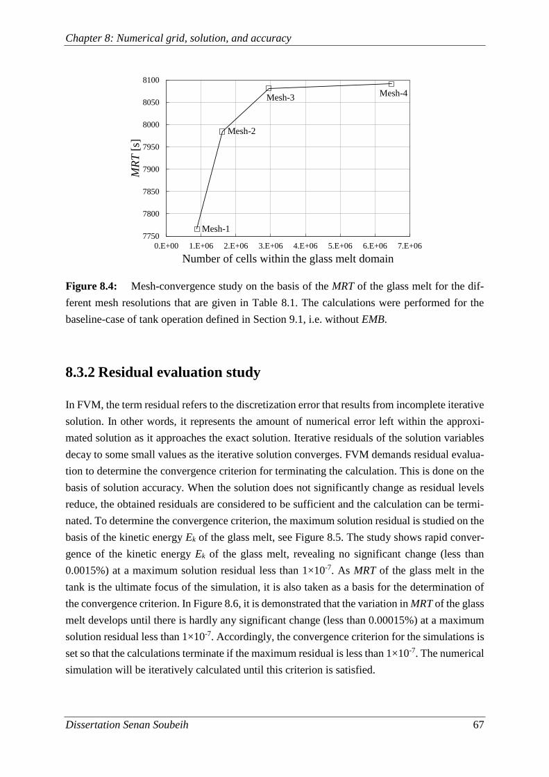
Chapter 8: Numerical grid, solution, and accuracy
Dissertation Senan Soubeih 67
8.3.2 Residual evaluation study
In FVM, the term residual refers to the discretization error that results from incomplete iterative
solution. In other words, it represents the amount of numerical error left within the approxi-
mated solution as it approaches the exact solution. Iterative residuals of the solution variables
decay to some small values as the iterative solution converges. FVM demands residual evalua-
tion to determine the convergence criterion for terminating the calculation. This is done on the
basis of solution accuracy. When the solution does not significantly change as residual levels
reduce, the obtained residuals are considered to be sufficient and the calculation can be termi-
nated. To determine the convergence criterion, the maximum solution residual is studied on the
basis of the kinetic energy Ek of the glass melt, see Figure 8.5. The study shows rapid conver-
gence of the kinetic energy Ek of the glass melt, revealing no significant change (less than
0.0015%) at a maximum solution residual less than 1×10⁻⁷. As MRT of the glass melt in the
tank is the ultimate focus of the simulation, it is also taken as a basis for the determination of
the convergence criterion. In Figure 8.6, it is demonstrated that the variation in MRT of the glass
melt develops until there is hardly any significant change (less than 0.00015%) at a maximum
solution residual less than 1×10⁻⁷. Accordingly, the convergence criterion for the simulations is
set so that the calculations terminate if the maximum residual is less than 1×10⁻⁷. The numerical
simulation will be iteratively calculated until this criterion is satisfied.
Figure 8.4: Mesh-convergence study on the basis of the MRT of the glass melt for the dif-
ferent mesh resolutions that are given in Table 8.1. The calculations were performed for the
baseline-case of tank operation defined in Section 9.1, i.e. without EMB.
7750
7800
7850
7900
7950
8000
8050
8100
0.E+00 1.E+06 2.E+06 3.E+06 4.E+06 5.E+06 6.E+06 7.E+06
MR
T[s
]
Number of cells within the glass melt domain
Mesh-1
Mesh-2
Mesh-3 Mesh-4
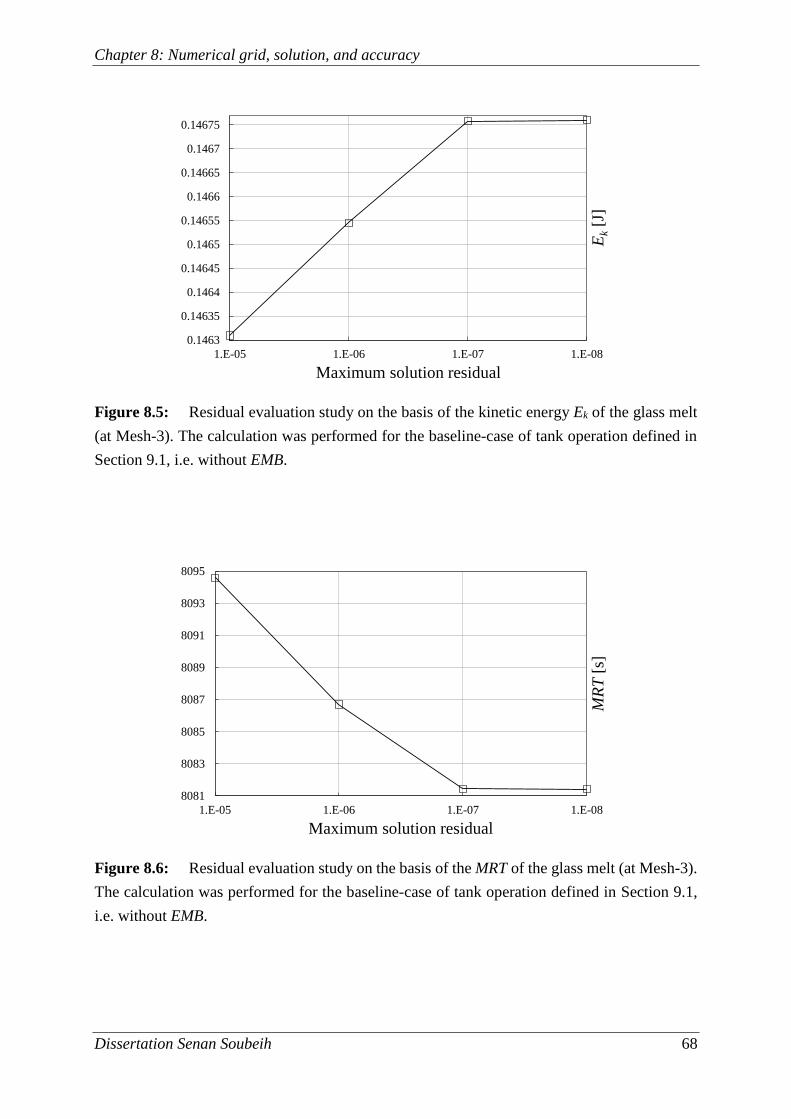
Chapter 8: Numerical grid, solution, and accuracy
Dissertation Senan Soubeih 68
Figure 8.5: Residual evaluation study on the basis of the kinetic energy Ek of the glass melt
(at Mesh-3). The calculation was performed for the baseline-case of tank operation defined in
Section 9.1, i.e. without EMB.
Figure 8.6: Residual evaluation study on the basis of the MRT of the glass melt (at Mesh-3).
The calculation was performed for the baseline-case of tank operation defined in Section 9.1,
i.e. without EMB.
0.1463
0.14635
0.1464
0.14645
0.1465
0.14655
0.1466
0.14665
0.1467
0.14675
1.E-081.E-071.E-061.E-05
Ek
[J]
Maximum solution residual
8081
8083
8085
8087
8089
8091
8093
8095
1.E-081.E-071.E-061.E-05
MR
T[s
]
Maximum solution residual
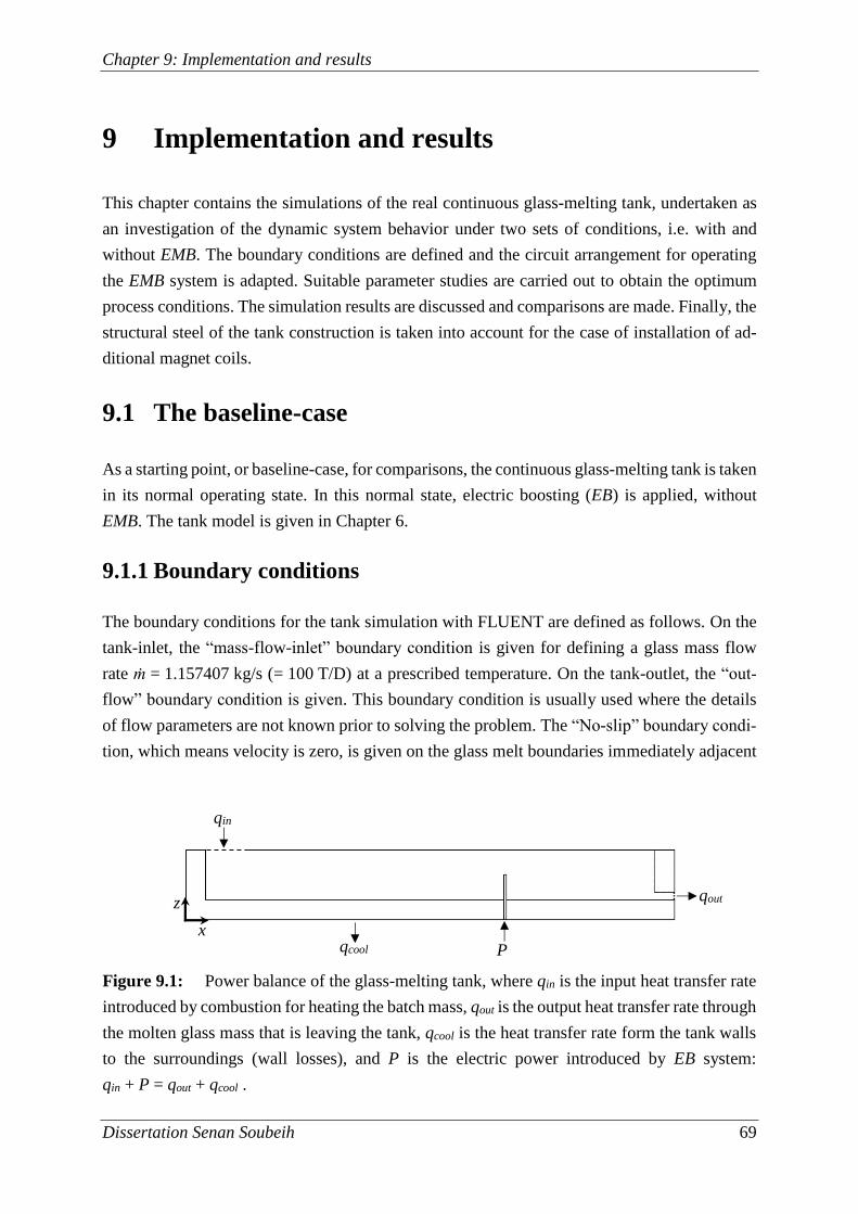
Chapter 9: Implementation and results
Dissertation Senan Soubeih 69
9 Implementation and results
This chapter contains the simulations of the real continuous glass-melting tank, undertaken as
an investigation of the dynamic system behavior under two sets of conditions, i.e. with and
without EMB. The boundary conditions are defined and the circuit arrangement for operating
the EMB system is adapted. Suitable parameter studies are carried out to obtain the optimum
process conditions. The simulation results are discussed and comparisons are made. Finally, the
structural steel of the tank construction is taken into account for the case of installation of ad-
ditional magnet coils.
9.1 The baseline-case
As a starting point, or baseline-case, for comparisons, the continuous glass-melting tank is taken
in its normal operating state. In this normal state, electric boosting (EB) is applied, without
EMB. The tank model is given in Chapter 6.
9.1.1 Boundary conditions
The boundary conditions for the tank simulation with FLUENT are defined as follows. On the
tank-inlet, the “mass-flow-inlet” boundary condition is given for defining a glass mass flow
rate ṁ = 1.157407 kg/s (= 100 T/D) at a prescribed temperature. On the tank-outlet, the “out-
flow” boundary condition is given. This boundary condition is usually used where the details
of flow parameters are not known prior to solving the problem. The “No-slip” boundary condi-
tion, which means velocity is zero, is given on the glass melt boundaries immediately adjacent
Figure 9.1: Power balance of the glass-melting tank, where qin is the input heat transfer rate
introduced by combustion for heating the batch mass, qout is the output heat transfer rate through
the molten glass mass that is leaving the tank, qcool is the heat transfer rate form the tank walls
to the surroundings (wall losses), and P is the electric power introduced by EB system:
qin + P = qout + qcool .
qin
qcool P
qout
x
z
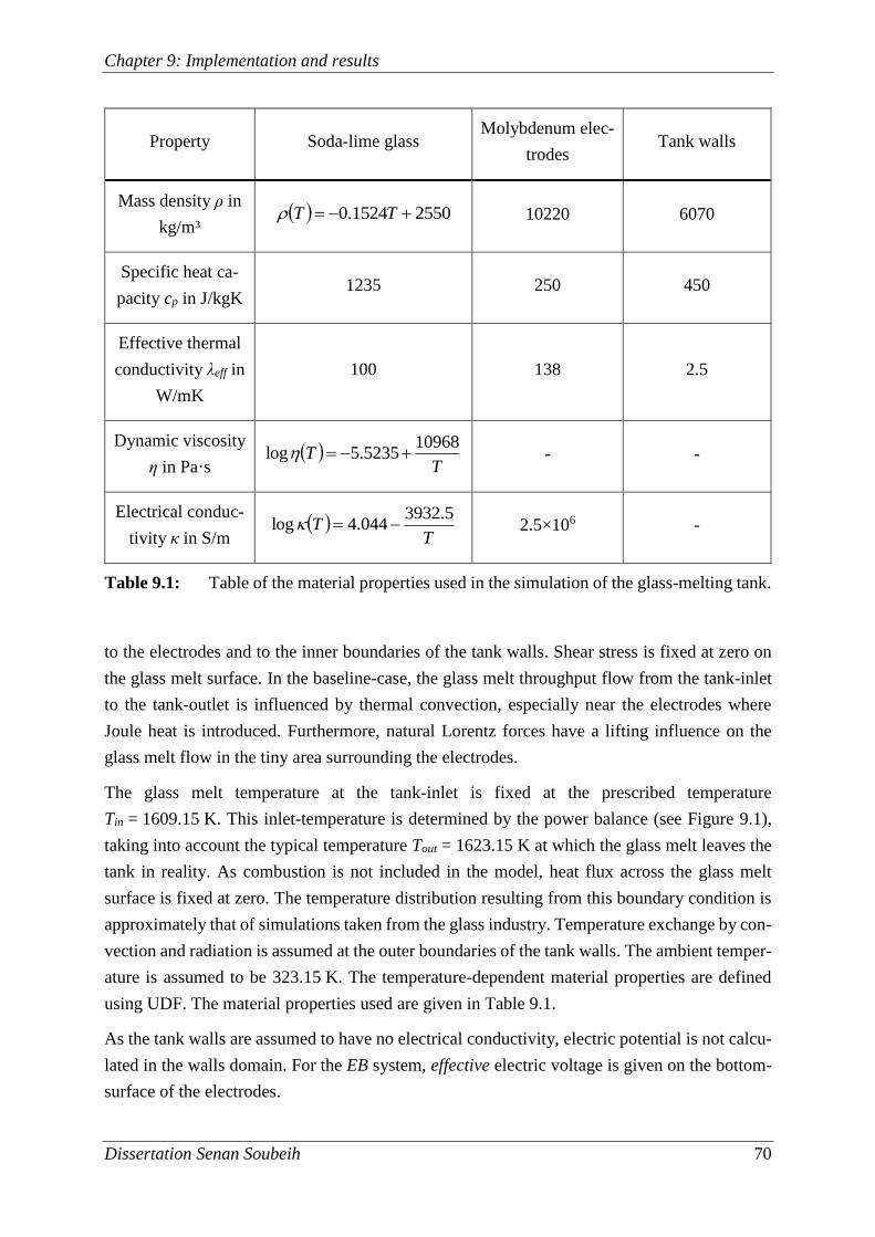
Chapter 9: Implementation and results
Dissertation Senan Soubeih 70
to the electrodes and to the inner boundaries of the tank walls. Shear stress is fixed at zero on
the glass melt surface. In the baseline-case, the glass melt throughput flow from the tank-inlet
to the tank-outlet is influenced by thermal convection, especially near the electrodes where
Joule heat is introduced. Furthermore, natural Lorentz forces have a lifting influence on the
glass melt flow in the tiny area surrounding the electrodes.
The glass melt temperature at the tank-inlet is fixed at the prescribed temperature
Tin = 1609.15 K. This inlet-temperature is determined by the power balance (see Figure 9.1),
taking into account the typical temperature Tout = 1623.15 K at which the glass melt leaves the
tank in reality. As combustion is not included in the model, heat flux across the glass melt
surface is fixed at zero. The temperature distribution resulting from this boundary condition is
approximately that of simulations taken from the glass industry. Temperature exchange by con-
vection and radiation is assumed at the outer boundaries of the tank walls. The ambient temper-
ature is assumed to be 323.15 K. The temperature-dependent material properties are defined
using UDF. The material properties used are given in Table 9.1.
As the tank walls are assumed to have no electrical conductivity, electric potential is not calcu-
lated in the walls domain. For the EB system, effective electric voltage is given on the bottom-
surface of the electrodes.
Property Soda-lime glass Molybdenum elec-
trodes Tank walls
Mass density ρ in
kg/m³ 25501524.0 TT 10220 6070
Specific heat ca-
pacity cp in J/kgK 1235 250 450
Effective thermal
conductivity λeff in
W/mK
100 138 2.5
Dynamic viscosity
η in Pa·s
TT
109685235.5log - -
Electrical conduc-
tivity κ in S/m
TT
5.3932044.4log 2.5×10⁶ -
Table 9.1: Table of the material properties used in the simulation of the glass-melting tank.
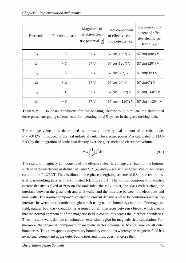
Chapter 9: Implementation and results
Dissertation Senan Soubeih 71
The voltage value is so determined as to result in the typical amount of electric power
P = 700 kW introduced in the real industrial tank. The electric power P is calculated in FLU-
ENT by the integration of Joule heat density over the glass melt and electrodes volume:
V
dVP21
J
(9.1)
The real and imaginary components of the effective electric voltage are fixed on the bottom-
surface of the electrodes as defined in Table 9.2. φRe and φIm are set using the “Value” boundary
condition in FLUENT. The distributed three-phase energizing scheme of EB in the real indus-
trial glass-melting tank is thus simulated (cf. Figure 3.3). The normal component of electric
current density is fixed at zero on the tank-inlet, the tank-outlet, the glass melt surface, the
interface between the glass melt and tank walls, and the interface between the electrodes and
tank walls. The normal component of electric current density is set to be continuous across the
interface between the electrodes and glass melt using natural boundary condition. For magnetic
field, natural boundary condition is assumed on all interfaces between objects, which means
that the normal component of the magnetic field is continuous across the interface boundaries.
Thus, the tank walls domain constitutes an extension region for magnetic field calculation. Fur-
thermore, the tangential component of magnetic vector potential is fixed at zero on all outer
boundaries. This corresponds to symmetry boundary conditions whereby the magnetic field has
no normal component at the outer boundaries and, thus, does not cross them.
Electrode Electrical phase
Magnitude of
effective elec-
tric potential
Real component
of effective elec-
tric potential φRe
Imaginary com-
ponent of effec-
tive electric po-
tential φIm
E1 – R 57 V 57 cos(180°) V 57 sin(180°) V
E2 + T 57 V 57 cos(120°) V 57 sin(120°) V
E3 – S 57 V 57 cos(60°) V 57 sin(60°) V
E4 + R 57 V 57 cos(0°) V 57 sin(0°) V
E5 – T 57 V 57 cos(– 60°) V 57 sin(– 60°) V
E6 + S 57 V 57 cos(– 120°) V 57 sin(– 120°) V
Table 9.2: Boundary conditions for the boosting electrodes to simulate the distributed
three-phase energizing scheme used for operating the EB system in the glass-melting tank.
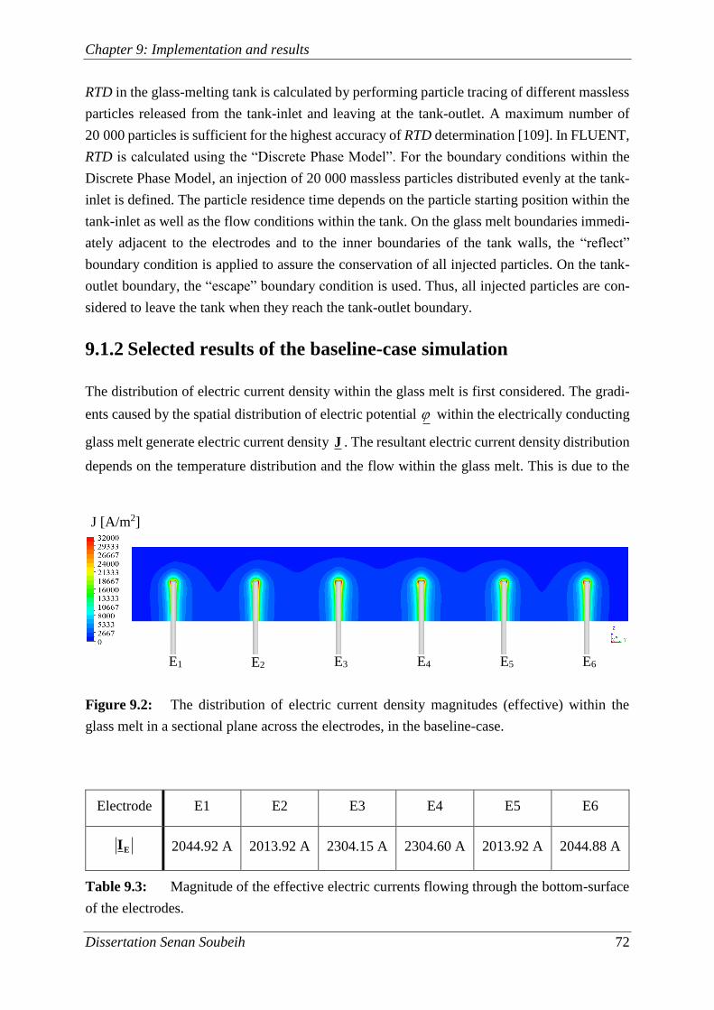
Chapter 9: Implementation and results
Dissertation Senan Soubeih 72
RTD in the glass-melting tank is calculated by performing particle tracing of different massless
particles released from the tank-inlet and leaving at the tank-outlet. A maximum number of
20 000 particles is sufficient for the highest accuracy of RTD determination [109]. In FLUENT,
RTD is calculated using the “Discrete Phase Model”. For the boundary conditions within the
Discrete Phase Model, an injection of 20 000 massless particles distributed evenly at the tank-
inlet is defined. The particle residence time depends on the particle starting position within the
tank-inlet as well as the flow conditions within the tank. On the glass melt boundaries immedi-
ately adjacent to the electrodes and to the inner boundaries of the tank walls, the “reflect”
boundary condition is applied to assure the conservation of all injected particles. On the tank-
outlet boundary, the “escape” boundary condition is used. Thus, all injected particles are con-
sidered to leave the tank when they reach the tank-outlet boundary.
9.1.2 Selected results of the baseline-case simulation
The distribution of electric current density within the glass melt is first considered. The gradi-
ents caused by the spatial distribution of electric potential within the electrically conducting
glass melt generate electric current density J . The resultant electric current density distribution
depends on the temperature distribution and the flow within the glass melt. This is due to the
Figure 9.2: The distribution of electric current density magnitudes (effective) within the
glass melt in a sectional plane across the electrodes, in the baseline-case.
Electrode E1 E2 E3 E4 E5 E6
EI 2044.92 A 2013.92 A 2304.15 A 2304.60 A 2013.92 A 2044.88 A
Table 9.3: Magnitude of the effective electric currents flowing through the bottom-surface
of the electrodes.
J [A/m2]
E1 E2 E3 E4 E5 E6
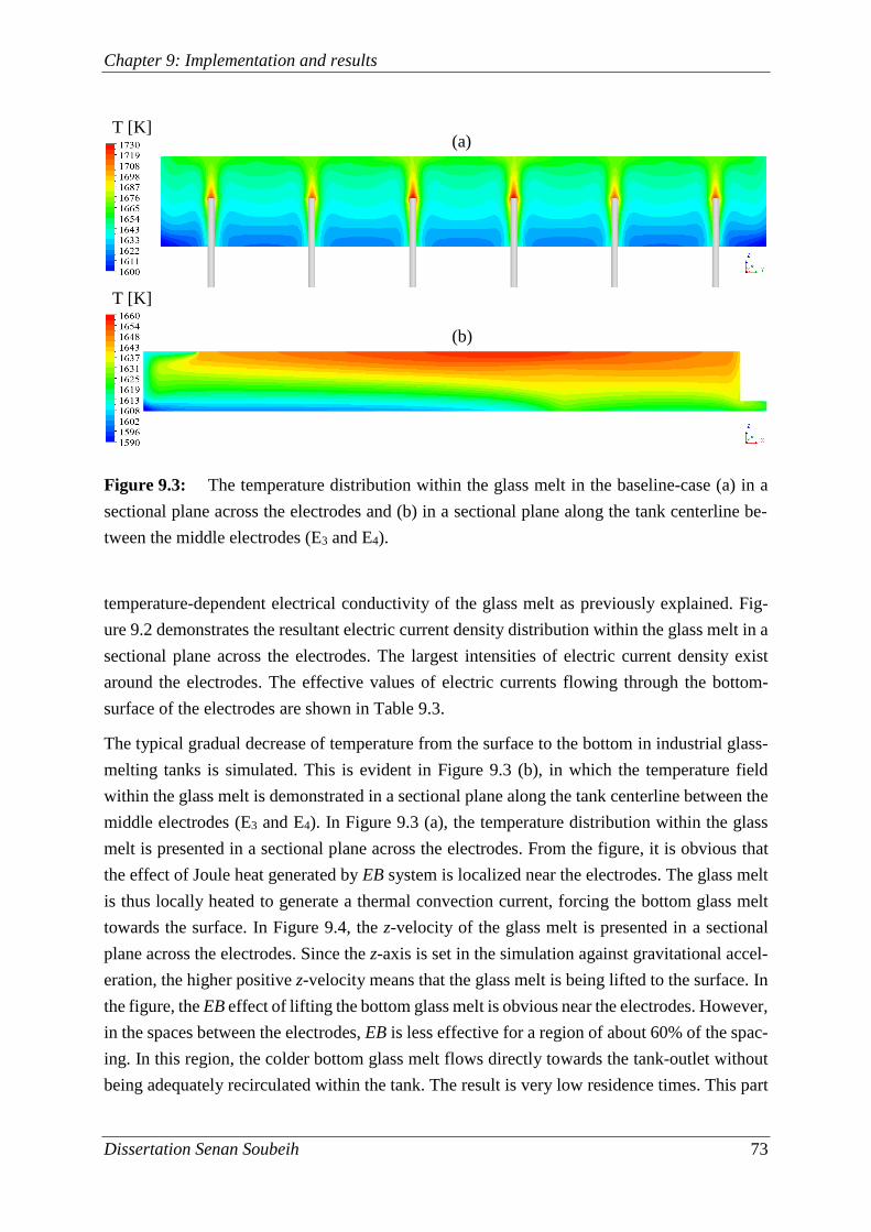
Chapter 9: Implementation and results
Dissertation Senan Soubeih 73
temperature-dependent electrical conductivity of the glass melt as previously explained. Fig-
ure 9.2 demonstrates the resultant electric current density distribution within the glass melt in a
sectional plane across the electrodes. The largest intensities of electric current density exist
around the electrodes. The effective values of electric currents flowing through the bottom-
surface of the electrodes are shown in Table 9.3.
The typical gradual decrease of temperature from the surface to the bottom in industrial glass-
melting tanks is simulated. This is evident in Figure 9.3 (b), in which the temperature field
within the glass melt is demonstrated in a sectional plane along the tank centerline between the
middle electrodes (E3 and E4). In Figure 9.3 (a), the temperature distribution within the glass
melt is presented in a sectional plane across the electrodes. From the figure, it is obvious that
the effect of Joule heat generated by EB system is localized near the electrodes. The glass melt
is thus locally heated to generate a thermal convection current, forcing the bottom glass melt
towards the surface. In Figure 9.4, the z-velocity of the glass melt is presented in a sectional
plane across the electrodes. Since the z-axis is set in the simulation against gravitational accel-
eration, the higher positive z-velocity means that the glass melt is being lifted to the surface. In
the figure, the EB effect of lifting the bottom glass melt is obvious near the electrodes. However,
in the spaces between the electrodes, EB is less effective for a region of about 60% of the spac-
ing. In this region, the colder bottom glass melt flows directly towards the tank-outlet without
being adequately recirculated within the tank. The result is very low residence times. This part
Figure 9.3: The temperature distribution within the glass melt in the baseline-case (a) in a
sectional plane across the electrodes and (b) in a sectional plane along the tank centerline be-
tween the middle electrodes (E3 and E4).
T [K]
T [K] (a)
(b)
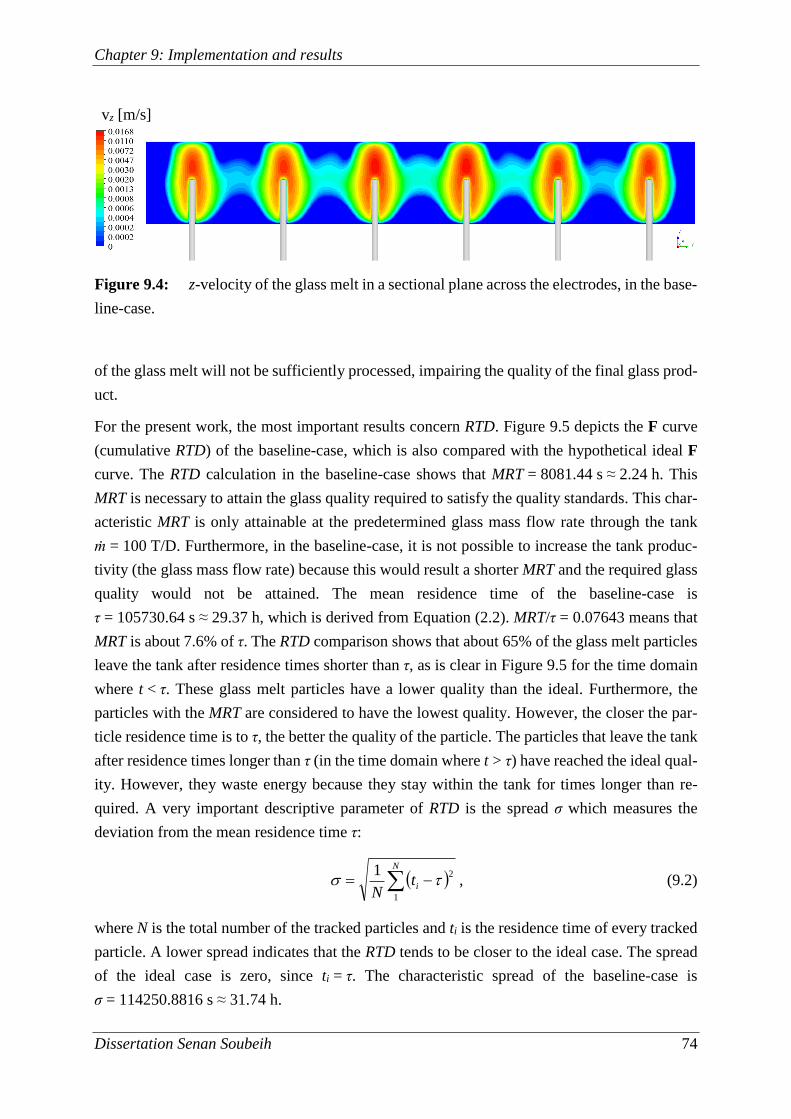
Chapter 9: Implementation and results
Dissertation Senan Soubeih 74
of the glass melt will not be sufficiently processed, impairing the quality of the final glass prod-
uct.
For the present work, the most important results concern RTD. Figure 9.5 depicts the F curve
(cumulative RTD) of the baseline-case, which is also compared with the hypothetical ideal F
curve. The RTD calculation in the baseline-case shows that MRT = 8081.44 s ≈ 2.24 h. This
MRT is necessary to attain the glass quality required to satisfy the quality standards. This char-
acteristic MRT is only attainable at the predetermined glass mass flow rate through the tank
ṁ = 100 T/D. Furthermore, in the baseline-case, it is not possible to increase the tank produc-
tivity (the glass mass flow rate) because this would result a shorter MRT and the required glass
quality would not be attained. The mean residence time of the baseline-case is
τ = 105730.64 s ≈ 29.37 h, which is derived from Equation (2.2). MRT/τ = 0.07643 means that
MRT is about 7.6% of τ. The RTD comparison shows that about 65% of the glass melt particles
leave the tank after residence times shorter than τ, as is clear in Figure 9.5 for the time domain
where t < τ. These glass melt particles have a lower quality than the ideal. Furthermore, the
particles with the MRT are considered to have the lowest quality. However, the closer the par-
ticle residence time is to τ, the better the quality of the particle. The particles that leave the tank
after residence times longer than τ (in the time domain where t > τ) have reached the ideal qual-
ity. However, they waste energy because they stay within the tank for times longer than re-
quired. A very important descriptive parameter of RTD is the spread σ which measures the
deviation from the mean residence time τ:
N
itN 1
21 , (9.2)
where N is the total number of the tracked particles and ti is the residence time of every tracked
particle. A lower spread indicates that the RTD tends to be closer to the ideal case. The spread
of the ideal case is zero, since ti = τ. The characteristic spread of the baseline-case is
σ = 114250.8816 s ≈ 31.74 h.
Figure 9.4: z-velocity of the glass melt in a sectional plane across the electrodes, in the base-
line-case.
vz [m/s]
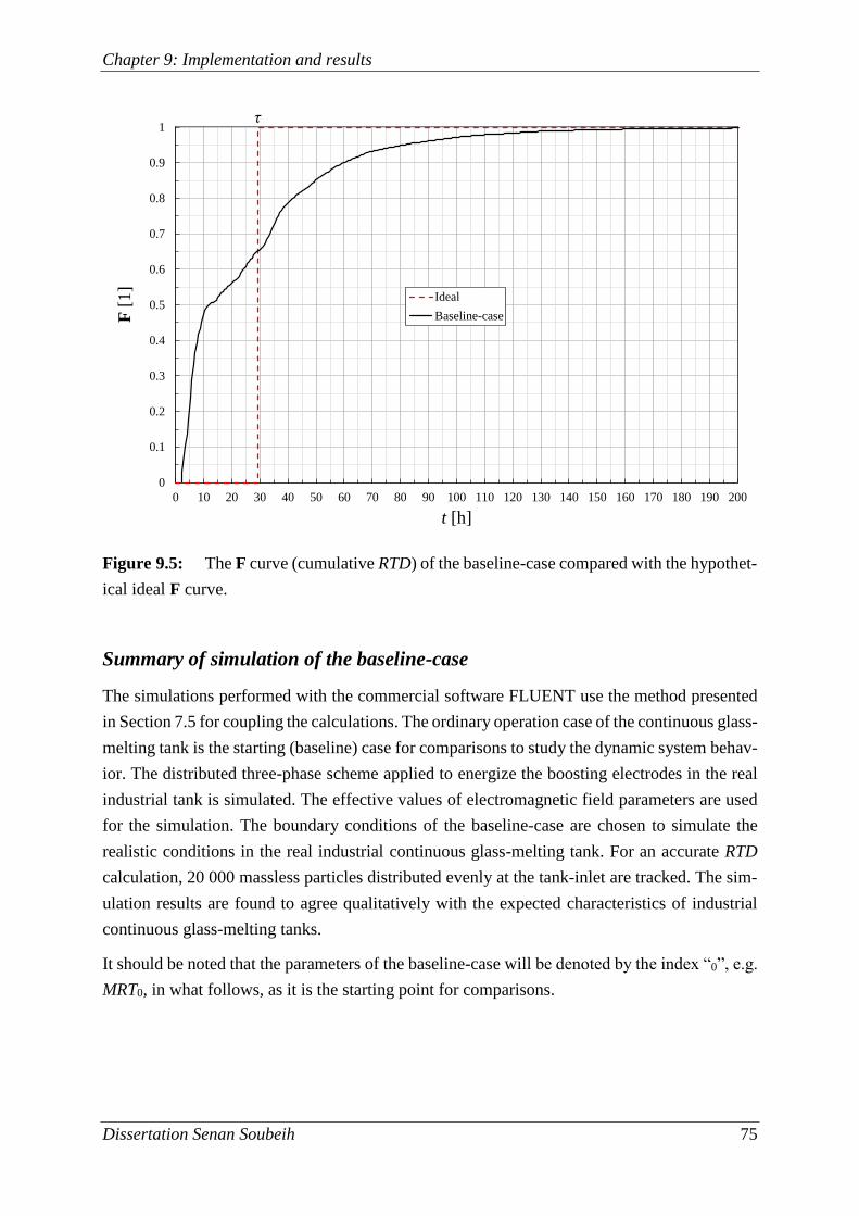
Chapter 9: Implementation and results
Dissertation Senan Soubeih 75
Summary of simulation of the baseline-case
The simulations performed with the commercial software FLUENT use the method presented
in Section 7.5 for coupling the calculations. The ordinary operation case of the continuous glass-
melting tank is the starting (baseline) case for comparisons to study the dynamic system behav-
ior. The distributed three-phase scheme applied to energize the boosting electrodes in the real
industrial tank is simulated. The effective values of electromagnetic field parameters are used
for the simulation. The boundary conditions of the baseline-case are chosen to simulate the
realistic conditions in the real industrial continuous glass-melting tank. For an accurate RTD
calculation, 20 000 massless particles distributed evenly at the tank-inlet are tracked. The sim-
ulation results are found to agree qualitatively with the expected characteristics of industrial
continuous glass-melting tanks.
It should be noted that the parameters of the baseline-case will be denoted by the index “0”, e.g.
MRT0, in what follows, as it is the starting point for comparisons.
Figure 9.5: The F curve (cumulative RTD) of the baseline-case compared with the hypothet-
ical ideal F curve.
0
0.1
0.2
0.3
0.4
0.5
0.6
0.7
0.8
0.9
1
0 10 20 30 40 50 60 70 80 90 100 110 120 130 140 150 160 170 180 190 200
F[1
]
t [h]
Ideal
Baseline-case
τ
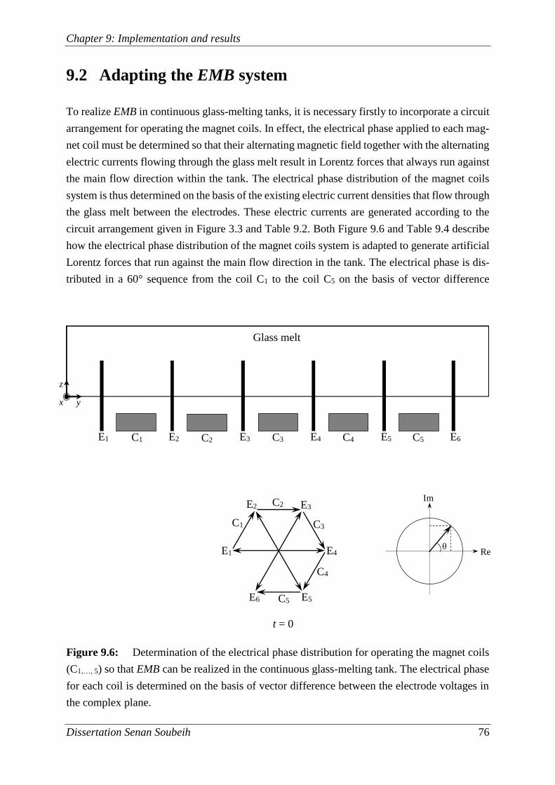
Chapter 9: Implementation and results
Dissertation Senan Soubeih 76
9.2 Adapting the EMB system
To realize EMB in continuous glass-melting tanks, it is necessary firstly to incorporate a circuit
arrangement for operating the magnet coils. In effect, the electrical phase applied to each mag-
net coil must be determined so that their alternating magnetic field together with the alternating
electric currents flowing through the glass melt result in Lorentz forces that always run against
the main flow direction within the tank. The electrical phase distribution of the magnet coils
system is thus determined on the basis of the existing electric current densities that flow through
the glass melt between the electrodes. These electric currents are generated according to the
circuit arrangement given in Figure 3.3 and Table 9.2. Both Figure 9.6 and Table 9.4 describe
how the electrical phase distribution of the magnet coils system is adapted to generate artificial
Lorentz forces that run against the main flow direction in the tank. The electrical phase is dis-
tributed in a 60° sequence from the coil C1 to the coil C5 on the basis of vector difference
Figure 9.6: Determination of the electrical phase distribution for operating the magnet coils
(C1,…, 5) so that EMB can be realized in the continuous glass-melting tank. The electrical phase
for each coil is determined on the basis of vector difference between the electrode voltages in
the complex plane.
Glass melt
E1
E2 E3
E4
E5 E6
E1 E2 E3 E4 E5 E6
C3
C2
C1
C4
C5
C1 C2 C3 C4 C5
y
z
x
t = 0
Re
Im
θ
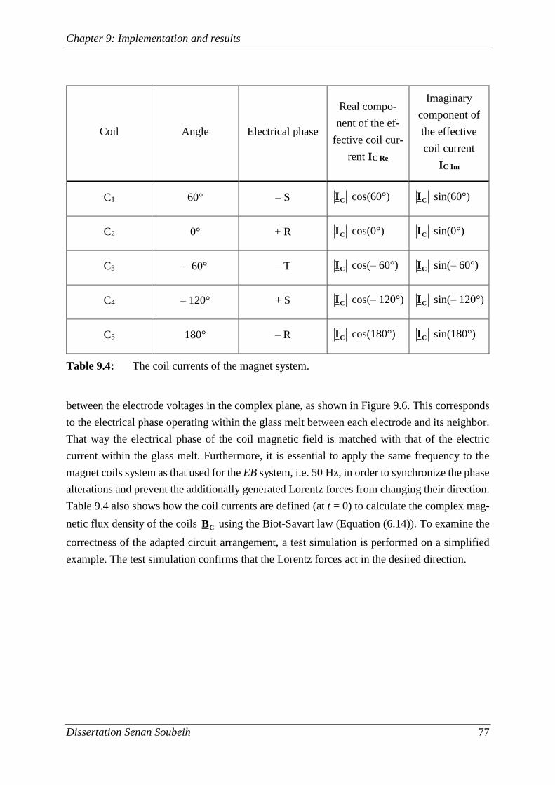
Chapter 9: Implementation and results
Dissertation Senan Soubeih 77
between the electrode voltages in the complex plane, as shown in Figure 9.6. This corresponds
to the electrical phase operating within the glass melt between each electrode and its neighbor.
That way the electrical phase of the coil magnetic field is matched with that of the electric
current within the glass melt. Furthermore, it is essential to apply the same frequency to the
magnet coils system as that used for the EB system, i.e. 50 Hz, in order to synchronize the phase
alterations and prevent the additionally generated Lorentz forces from changing their direction.
Table 9.4 also shows how the coil currents are defined (at t = 0) to calculate the complex mag-
netic flux density of the coils CB using the Biot-Savart law (Equation (6.14)). To examine the
correctness of the adapted circuit arrangement, a test simulation is performed on a simplified
example. The test simulation confirms that the Lorentz forces act in the desired direction.
Coil Angle Electrical phase
Real compo-
nent of the ef-
fective coil cur-
rent IC Re
Imaginary
component of
the effective
coil current
IC Im
C1 60° – S CI cos(60°) CI sin(60°)
C2 0° + R CI cos(0°) CI sin(0°)
C3 – 60° – T CI cos(– 60°) CI sin(– 60°)
C4 – 120° + S CI cos(– 120°) CI sin(– 120°)
C5 180° – R CI cos(180°) CI sin(180°)
Table 9.4: The coil currents of the magnet system.
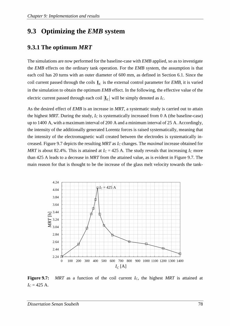
Chapter 9: Implementation and results
Dissertation Senan Soubeih 78
9.3 Optimizing the EMB system
9.3.1 The optimum MRT
The simulations are now performed for the baseline-case with EMB applied, so as to investigate
the EMB effects on the ordinary tank operation. For the EMB system, the assumption is that
each coil has 20 turns with an outer diameter of 600 mm, as defined in Section 6.1. Since the
coil current passed through the coils CI is the external control parameter for EMB, it is varied
in the simulation to obtain the optimum EMB effect. In the following, the effective value of the
electric current passed through each coil CI will be simply denoted as IC.
As the desired effect of EMB is an increase in MRT, a systematic study is carried out to attain
the highest MRT. During the study, IC is systematically increased from 0 A (the baseline-case)
up to 1400 A, with a maximum interval of 200 A and a minimum interval of 25 A. Accordingly,
the intensity of the additionally generated Lorentz forces is raised systematically, meaning that
the intensity of the electromagnetic wall created between the electrodes is systematically in-
creased. Figure 9.7 depicts the resulting MRT as IC changes. The maximal increase obtained for
MRT is about 82.4%. This is attained at IC = 425 A. The study reveals that increasing IC more
than 425 A leads to a decrease in MRT from the attained value, as is evident in Figure 9.7. The
main reason for that is thought to be the increase of the glass melt velocity towards the tank-
Figure 9.7: MRT as a function of the coil current IC, the highest MRT is attained at
IC = 425 A.
2.24
2.44
2.64
2.84
3.04
3.24
3.44
3.64
3.84
4.04
4.24
0 100 200 300 400 500 600 700 800 900 1000 1100 1200 1300 1400
MR
T[h
]
IC [A]
IC = 425 A
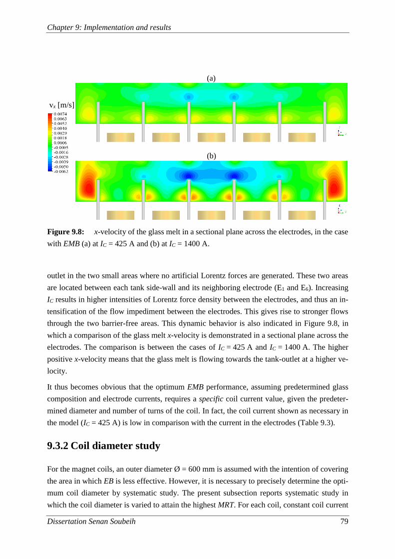
Chapter 9: Implementation and results
Dissertation Senan Soubeih 79
outlet in the two small areas where no artificial Lorentz forces are generated. These two areas
are located between each tank side-wall and its neighboring electrode (E1 and E6). Increasing
IC results in higher intensities of Lorentz force density between the electrodes, and thus an in-
tensification of the flow impediment between the electrodes. This gives rise to stronger flows
through the two barrier-free areas. This dynamic behavior is also indicated in Figure 9.8, in
which a comparison of the glass melt x-velocity is demonstrated in a sectional plane across the
electrodes. The comparison is between the cases of IC = 425 A and IC = 1400 A. The higher
positive x-velocity means that the glass melt is flowing towards the tank-outlet at a higher ve-
locity.
It thus becomes obvious that the optimum EMB performance, assuming predetermined glass
composition and electrode currents, requires a specific coil current value, given the predeter-
mined diameter and number of turns of the coil. In fact, the coil current shown as necessary in
the model (IC = 425 A) is low in comparison with the current in the electrodes (Table 9.3).
9.3.2 Coil diameter study
For the magnet coils, an outer diameter Ø = 600 mm is assumed with the intention of covering
the area in which EB is less effective. However, it is necessary to precisely determine the opti-
mum coil diameter by systematic study. The present subsection reports systematic study in
which the coil diameter is varied to attain the highest MRT. For each coil, constant coil current
Figure 9.8: x-velocity of the glass melt in a sectional plane across the electrodes, in the case
with EMB (a) at IC = 425 A and (b) at IC = 1400 A.
vx [m/s]
(a)
(b)
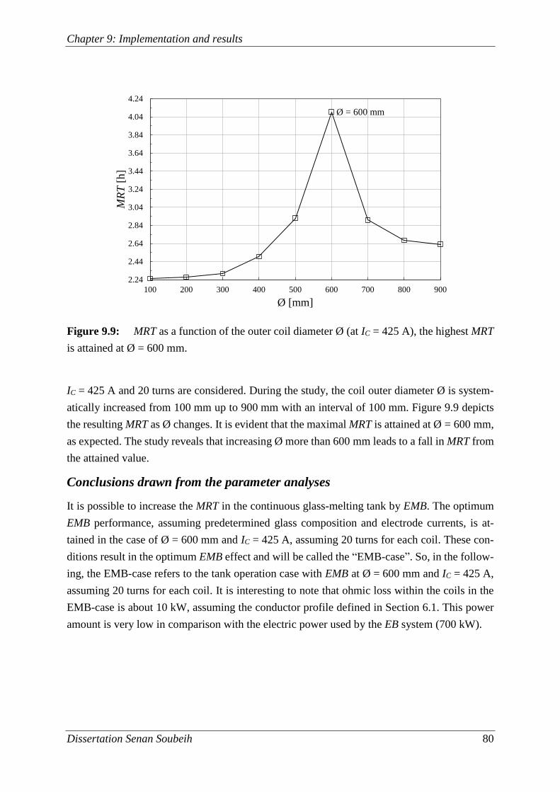
Chapter 9: Implementation and results
Dissertation Senan Soubeih 80
IC = 425 A and 20 turns are considered. During the study, the coil outer diameter Ø is system-
atically increased from 100 mm up to 900 mm with an interval of 100 mm. Figure 9.9 depicts
the resulting MRT as Ø changes. It is evident that the maximal MRT is attained at Ø = 600 mm,
as expected. The study reveals that increasing Ø more than 600 mm leads to a fall in MRT from
the attained value.
Conclusions drawn from the parameter analyses
It is possible to increase the MRT in the continuous glass-melting tank by EMB. The optimum
EMB performance, assuming predetermined glass composition and electrode currents, is at-
tained in the case of Ø = 600 mm and IC = 425 A, assuming 20 turns for each coil. These con-
ditions result in the optimum EMB effect and will be called the “EMB-case”. So, in the follow-
ing, the EMB-case refers to the tank operation case with EMB at Ø = 600 mm and IC = 425 A,
assuming 20 turns for each coil. It is interesting to note that ohmic loss within the coils in the
EMB-case is about 10 kW, assuming the conductor profile defined in Section 6.1. This power
amount is very low in comparison with the electric power used by the EB system (700 kW).
Figure 9.9: MRT as a function of the outer coil diameter Ø (at IC = 425 A), the highest MRT
is attained at Ø = 600 mm.
2.24
2.44
2.64
2.84
3.04
3.24
3.44
3.64
3.84
4.04
4.24
100 200 300 400 500 600 700 800 900
MR
T[h
]
Ø [mm]
Ø = 600 mm
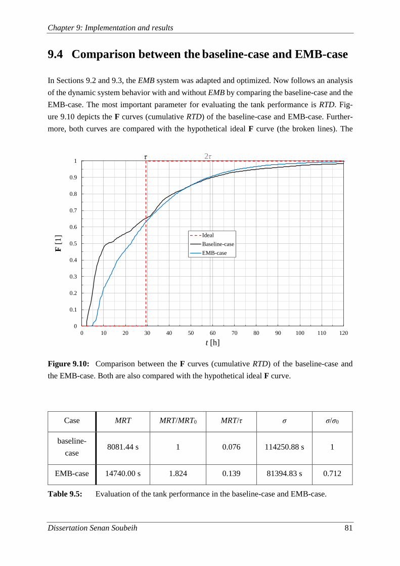
Chapter 9: Implementation and results
Dissertation Senan Soubeih 81
9.4 Comparison between the baseline-case and EMB-case
In Sections 9.2 and 9.3, the EMB system was adapted and optimized. Now follows an analysis
of the dynamic system behavior with and without EMB by comparing the baseline-case and the
EMB-case. The most important parameter for evaluating the tank performance is RTD. Fig-
ure 9.10 depicts the F curves (cumulative RTD) of the baseline-case and EMB-case. Further-
more, both curves are compared with the hypothetical ideal F curve (the broken lines). The
Figure 9.10: Comparison between the F curves (cumulative RTD) of the baseline-case and
the EMB-case. Both are also compared with the hypothetical ideal F curve.
Case MRT MRT/MRT0 MRT/τ σ σ/σ0
baseline-
case 8081.44 s 1 0.076 114250.88 s 1
EMB-case 14740.00 s 1.824 0.139 81394.83 s 0.712
Table 9.5: Evaluation of the tank performance in the baseline-case and EMB-case.
0
0.1
0.2
0.3
0.4
0.5
0.6
0.7
0.8
0.9
1
0 10 20 30 40 50 60 70 80 90 100 110 120
F[1
]
t [h]
Ideal
Baseline-case
EMB-case
τ 2τ

Chapter 9: Implementation and results
Dissertation Senan Soubeih 82
mean residence time τ is the same for both cases, being defined by Equation (2.2). MRT of the
baseline-case is about 7.6% of τ, while that of the EMB-case is about 13.9% of τ. The RTD
comparative analysis shows that in the EMB-case, MRT is increased by about 82.4%. Moreover,
the RTD comparison in Figure 9.10 shows that about 15% of the glass melt particles in the
baseline-case have residence times that are lower than the MRT of the EMB-case. These glass
melt particles have quality lower than the minimum quality in the EMB-case. In the time do-
main where t < τ, the EMB-case allows fewer particles to leave the tank, so that the glass melt
will have a longer processing time and consequently a better quality. Moreover, if the time
domain exceeds twice the mean residence time t > 2τ, the EMB-case allows more particles to
leave the tank, shortening the unnecessary processing. The EMB-case has thus a spread σ that
is reduced by about 28.8%. In Figure 9.10, it is obvious how the F curve (cumulative RTD) is
brought closer to the ideal case by EMB. As a result, the timed distribution of the energy con-
sumed will be more homogeneous and, consequently, the glass quality will be enhanced. The
tank performance evaluation in the baseline-case and EMB-case is summarized in Table 9.5.
Figure 9.11 presents a magnitude comparison of the magnetic flux density distribution within
the glass melt in a vertical plane across the electrodes. The comparison is between the baseline-
case and EMB-case. In both cases, the eigenfield induced by the electrode currents has similar
intensities surrounding the electrodes. In the EMB-case, the additional magnetic flux density
generated by the coils (at IC = 425 A) between the electrodes can be distinguished. This mag-
netic flux density has a maximum intensity of about 6 mT at the bottom of the glass bath. The
Figure 9.11: The distribution of magnetic flux density magnitudes (effective) within the glass
melt in a sectional plane across the electrodes (a) in the baseline-case and (b) in the EMB-case.
B [T]
(a)
(b)
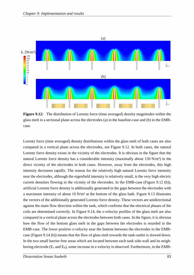
Chapter 9: Implementation and results
Dissertation Senan Soubeih 83
Lorentz force (time averaged) density distributions within the glass melt of both cases are also
compared in a vertical plane across the electrodes, see Figure 9.12. In both cases, the natural
Lorentz force density exists in the vicinity of the electrodes. It is obvious in the figure that the
natural Lorentz force density has a considerable intensity (maximally about 150 N/m³) in the
direct vicinity of the electrodes in both cases. However, away from the electrodes, this high
intensity decreases rapidly. The reason for the relatively high natural Lorentz force intensity
near the electrodes, although the eigenfield intensity is relatively small, is the very high electric
current densities flowing in the vicinity of the electrodes. In the EMB-case (Figure 9.12 (b)),
artificial Lorentz force density is additionally generated in the gaps between the electrodes with
a maximum intensity of about 10 N/m³ at the bottom of the glass bath. Figure 9.13 illustrates
the vectors of the additionally generated Lorentz force density. These vectors are unidirectional
against the main flow direction within the tank, which confirms that the electrical phases of the
coils are determined correctly. In Figure 9.14, the x-velocity profiles of the glass melt are also
compared in a vertical plane across the electrodes between both cases. In the figure, it is obvious
how the flow of the bottom glass melt in the gaps between the electrodes is retarded in the
EMB-case. The lower positive x-velocity near the bottom between the electrodes in the EMB-
case (Figure 9.14 (b)) means that the flow of glass melt towards the tank-outlet is slowed down.
In the two small barrier-free areas which are located between each tank side-wall and its neigh-
boring electrode (E1 and E6), some increase in x-velocity is observed. Furthermore, in the EMB-
Figure 9.12: The distribution of Lorentz force (time averaged) density magnitudes within the
glass melt in a sectional plane across the electrodes (a) in the baseline-case and (b) in the EMB-
case.
fL [N/m³]
(a)
(b)
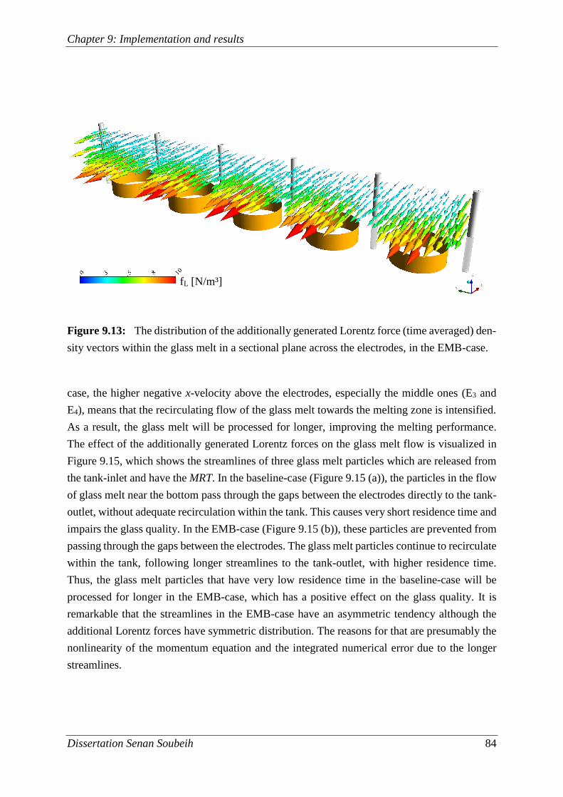
Chapter 9: Implementation and results
Dissertation Senan Soubeih 84
case, the higher negative x-velocity above the electrodes, especially the middle ones (E3 and
E4), means that the recirculating flow of the glass melt towards the melting zone is intensified.
As a result, the glass melt will be processed for longer, improving the melting performance.
The effect of the additionally generated Lorentz forces on the glass melt flow is visualized in
Figure 9.15, which shows the streamlines of three glass melt particles which are released from
the tank-inlet and have the MRT. In the baseline-case (Figure 9.15 (a)), the particles in the flow
of glass melt near the bottom pass through the gaps between the electrodes directly to the tank-
outlet, without adequate recirculation within the tank. This causes very short residence time and
impairs the glass quality. In the EMB-case (Figure 9.15 (b)), these particles are prevented from
passing through the gaps between the electrodes. The glass melt particles continue to recirculate
within the tank, following longer streamlines to the tank-outlet, with higher residence time.
Thus, the glass melt particles that have very low residence time in the baseline-case will be
processed for longer in the EMB-case, which has a positive effect on the glass quality. It is
remarkable that the streamlines in the EMB-case have an asymmetric tendency although the
additional Lorentz forces have symmetric distribution. The reasons for that are presumably the
nonlinearity of the momentum equation and the integrated numerical error due to the longer
streamlines.
Figure 9.13: The distribution of the additionally generated Lorentz force (time averaged) den-
sity vectors within the glass melt in a sectional plane across the electrodes, in the EMB-case.
fL [N/m³]
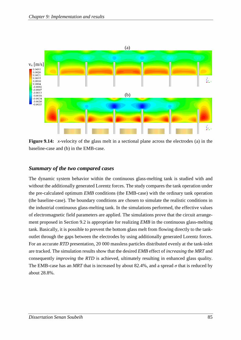
Chapter 9: Implementation and results
Dissertation Senan Soubeih 85
Summary of the two compared cases
The dynamic system behavior within the continuous glass-melting tank is studied with and
without the additionally generated Lorentz forces. The study compares the tank operation under
the pre-calculated optimum EMB conditions (the EMB-case) with the ordinary tank operation
(the baseline-case). The boundary conditions are chosen to simulate the realistic conditions in
the industrial continuous glass-melting tank. In the simulations performed, the effective values
of electromagnetic field parameters are applied. The simulations prove that the circuit arrange-
ment proposed in Section 9.2 is appropriate for realizing EMB in the continuous glass-melting
tank. Basically, it is possible to prevent the bottom glass melt from flowing directly to the tank-
outlet through the gaps between the electrodes by using additionally generated Lorentz forces.
For an accurate RTD presentation, 20 000 massless particles distributed evenly at the tank-inlet
are tracked. The simulation results show that the desired EMB effect of increasing the MRT and
consequently improving the RTD is achieved, ultimately resulting in enhanced glass quality.
The EMB-case has an MRT that is increased by about 82.4%, and a spread σ that is reduced by
about 28.8%.
Figure 9.14: x-velocity of the glass melt in a sectional plane across the electrodes (a) in the
baseline-case and (b) in the EMB-case.
vx [m/s]
(a)
(b)
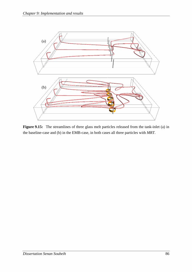
Chapter 9: Implementation and results
Dissertation Senan Soubeih 86
Figure 9.15: The streamlines of three glass melt particles released from the tank-inlet (a) in
the baseline-case and (b) in the EMB-case, in both cases all three particles with MRT.
(a)
(b)
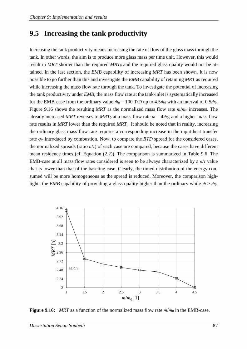
Chapter 9: Implementation and results
Dissertation Senan Soubeih 87
9.5 Increasing the tank productivity
Increasing the tank productivity means increasing the rate of flow of the glass mass through the
tank. In other words, the aim is to produce more glass mass per time unit. However, this would
result in MRT shorter than the required MRT0 and the required glass quality would not be at-
tained. In the last section, the EMB capability of increasing MRT has been shown. It is now
possible to go further than this and investigate the EMB capability of retaining MRT as required
while increasing the mass flow rate through the tank. To investigate the potential of increasing
the tank productivity under EMB, the mass flow rate at the tank-inlet is systematically increased
for the EMB-case from the ordinary value ṁ0 = 100 T/D up to 4.5ṁ0 with an interval of 0.5ṁ0.
Figure 9.16 shows the resulting MRT as the normalized mass flow rate ṁ/ṁ0 increases. The
already increased MRT reverses to MRT0 at a mass flow rate ṁ = 4ṁ0, and a higher mass flow
rate results in MRT lower than the required MRT0. It should be noted that in reality, increasing
the ordinary glass mass flow rate requires a corresponding increase in the input heat transfer
rate qin introduced by combustion. Now, to compare the RTD spread for the considered cases,
the normalized spreads (ratio σ/τ) of each case are compared, because the cases have different
mean residence times (cf. Equation (2.2)). The comparison is summarized in Table 9.6. The
EMB-case at all mass flow rates considered is seen to be always characterized by a σ/τ value
that is lower than that of the baseline-case. Clearly, the timed distribution of the energy con-
sumed will be more homogeneous as the spread is reduced. Moreover, the comparison high-
lights the EMB capability of providing a glass quality higher than the ordinary while ṁ > ṁ0.
Figure 9.16: MRT as a function of the normalized mass flow rate ṁ/ṁ0 in the EMB-case.
2
2.24
2.48
2.72
2.96
3.2
3.44
3.68
3.92
4.16
1 1.5 2 2.5 3 3.5 4 4.5
MR
T[h
]
ṁ/ṁ0 [1]
MRT0
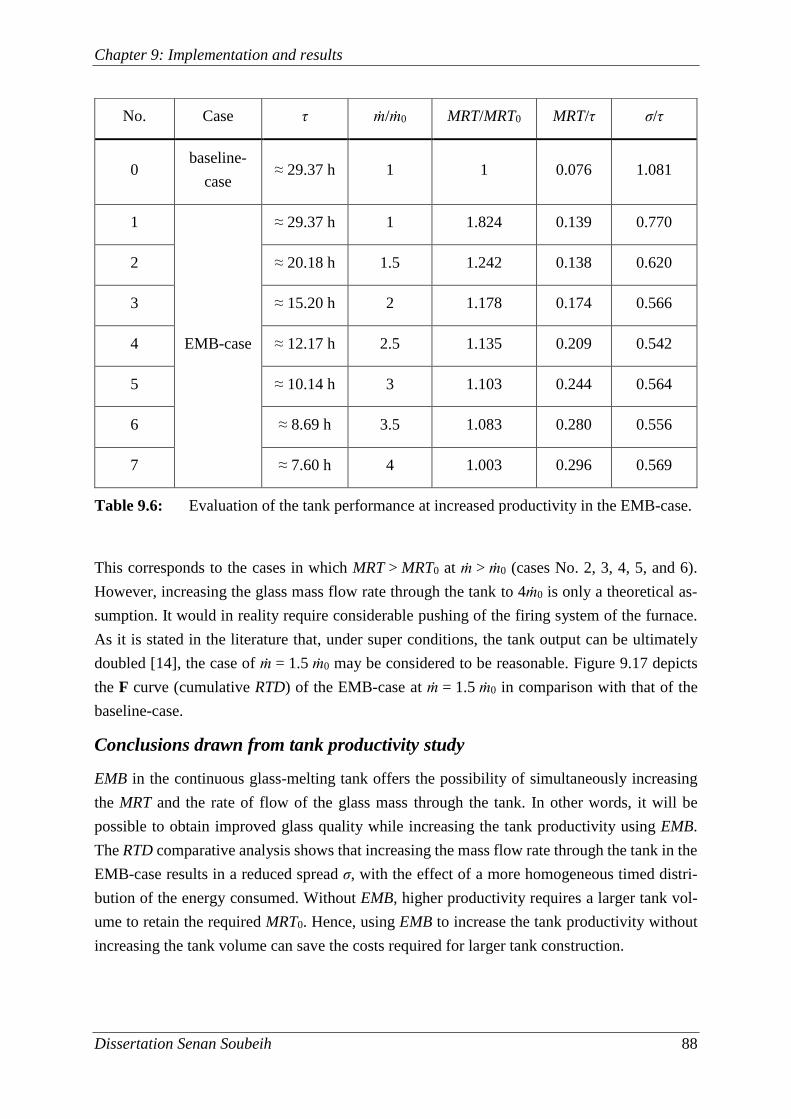
Chapter 9: Implementation and results
Dissertation Senan Soubeih 88
This corresponds to the cases in which MRT > MRT0 at ṁ > ṁ0 (cases No. 2, 3, 4, 5, and 6).
However, increasing the glass mass flow rate through the tank to 4ṁ0 is only a theoretical as-
sumption. It would in reality require considerable pushing of the firing system of the furnace.
As it is stated in the literature that, under super conditions, the tank output can be ultimately
doubled [14], the case of ṁ = 1.5 ṁ0 may be considered to be reasonable. Figure 9.17 depicts
the F curve (cumulative RTD) of the EMB-case at ṁ = 1.5 ṁ0 in comparison with that of the
baseline-case.
Conclusions drawn from tank productivity study
EMB in the continuous glass-melting tank offers the possibility of simultaneously increasing
the MRT and the rate of flow of the glass mass through the tank. In other words, it will be
possible to obtain improved glass quality while increasing the tank productivity using EMB.
The RTD comparative analysis shows that increasing the mass flow rate through the tank in the
EMB-case results in a reduced spread σ, with the effect of a more homogeneous timed distri-
bution of the energy consumed. Without EMB, higher productivity requires a larger tank vol-
ume to retain the required MRT0. Hence, using EMB to increase the tank productivity without
increasing the tank volume can save the costs required for larger tank construction.
No. Case τ ṁ/ṁ0 MRT/MRT0 MRT/τ σ/τ
0 baseline-
case ≈ 29.37 h 1 1 0.076 1.081
1
EMB-case
≈ 29.37 h 1 1.824 0.139 0.770
2 ≈ 20.18 h 1.5 1.242 0.138 0.620
3 ≈ 15.20 h 2 1.178 0.174 0.566
4 ≈ 12.17 h 2.5 1.135 0.209 0.542
5 ≈ 10.14 h 3 1.103 0.244 0.564
6 ≈ 8.69 h 3.5 1.083 0.280 0.556
7 ≈ 7.60 h 4 1.003 0.296 0.569
Table 9.6: Evaluation of the tank performance at increased productivity in the EMB-case.
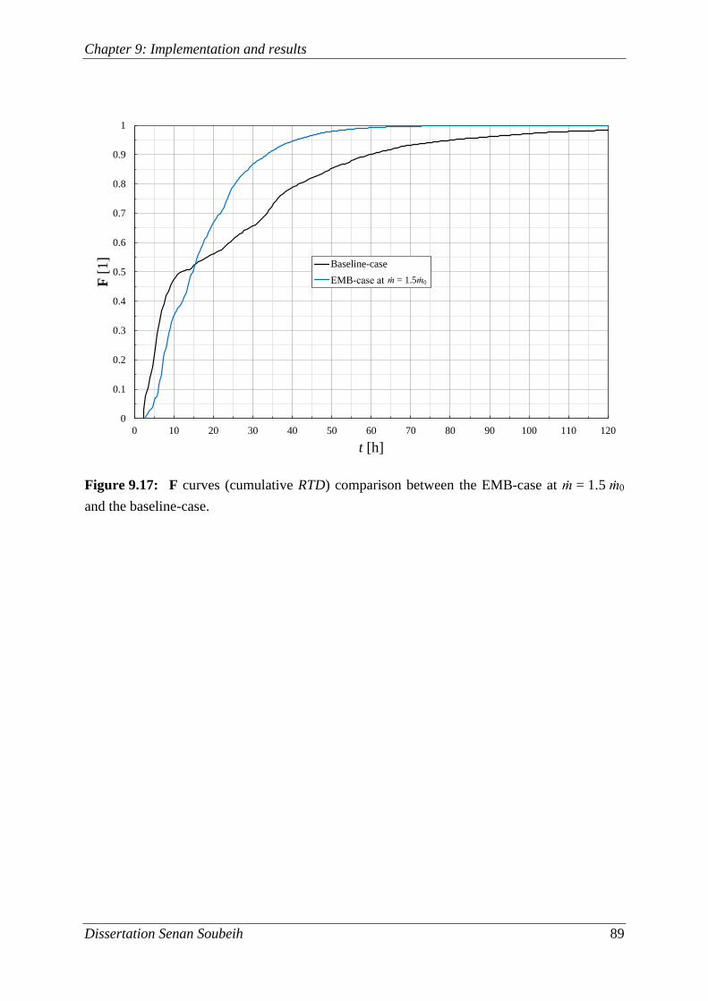
Chapter 9: Implementation and results
Dissertation Senan Soubeih 89
Figure 9.17: F curves (cumulative RTD) comparison between the EMB-case at ṁ = 1.5 ṁ0
and the baseline-case.
0
0.1
0.2
0.3
0.4
0.5
0.6
0.7
0.8
0.9
1
0 10 20 30 40 50 60 70 80 90 100 110 120
F[1
]
t [h]
Baseline-case
EMB-case at ṁ=1.5ṁ₀
ṁ = 1.5ṁ0
Chapter 9: Implementation and results
Dissertation Senan Soubeih 90
9.6 Increasing the tank thermal efficiency
In the ordinary tank operation case, if higher tank productivity is required, a larger tank volume
should be used to attain the required MRT0. This gives rise to higher thermal energy exchange
with the surroundings through the tank walls, cf. Equations (6.21) and (6.22), so that the wall
losses qcool will increase. EMB offers the possibility of increasing the tank productivity without
increasing its volume, thus keeping the wall losses qcool constant. This is to be interpreted as
energy saving that is evaluated by the tank thermal efficiency. The present section is concerned
with the theoretical investigation of how the tank thermal efficiency is improved by increasing
the tank productivity under EMB.
The ordinary tank thermal efficiency is calculated by
coolout
outth
q
0
00 , this also gives 0
0
0out
th
outcool q
. (9.3)
Under EMB, the ordinary tank output can be increased by the factor ṁ/ṁ0:
0
0
outout qm
mq
, (9.4)
where in the theoretical study 1 ≤ ṁ/ṁ0 ≤ 4.
The tank thermal efficiency resulting from an increased output will be
coolout
outth
q
. (9.5)
If qcool and qout (Equations (9.3) and (9.4) respectively) are substituted in Equation (9.5), the
resulting equation is
11
00
0
th
th
m
m
m
m
. (9.6)
Equation (9.6) gives the relation between the tank thermal efficiency and the increased produc-
tivity. The ordinary thermal efficiency of the tank under consideration is assumed ηth0 = 0.75.
Now, the potential improvement in tank thermal efficiency can be investigated by increasing
the ratio ṁ/ṁ0 systematically. The ratio ṁ/ṁ0 is raised from 1 up to 4 at intervals of 0.5, as
described in the last section. Figure 9.18 depicts how the tank thermal efficiency ηth in the
EMB-case increases together with the factor ṁ/ṁ0 according to Equation (9.6). The details of
the studied cases are also presented in Table 9.7. The cases at 1.5ṁ0 and 2ṁ0 can be considered
to be realistic. The thermal efficiency in these two cases has been increased by 9.3 % and 14.7%
respectively, which is advantageous in both economic and environmental terms. It should be
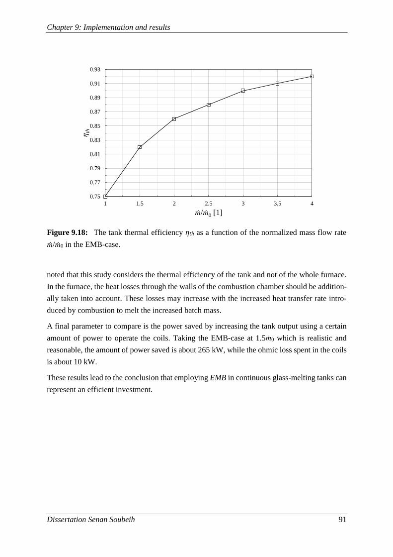
Chapter 9: Implementation and results
Dissertation Senan Soubeih 91
noted that this study considers the thermal efficiency of the tank and not of the whole furnace.
In the furnace, the heat losses through the walls of the combustion chamber should be addition-
ally taken into account. These losses may increase with the increased heat transfer rate intro-
duced by combustion to melt the increased batch mass.
A final parameter to compare is the power saved by increasing the tank output using a certain
amount of power to operate the coils. Taking the EMB-case at 1.5ṁ0 which is realistic and
reasonable, the amount of power saved is about 265 kW, while the ohmic loss spent in the coils
is about 10 kW.
These results lead to the conclusion that employing EMB in continuous glass-melting tanks can
represent an efficient investment.
Figure 9.18: The tank thermal efficiency ηth as a function of the normalized mass flow rate
ṁ/ṁ0 in the EMB-case.
0.75
0.77
0.79
0.81
0.83
0.85
0.87
0.89
0.91
0.93
1 1.5 2 2.5 3 3.5 4
ηth
ṁ/ṁ0 [1]
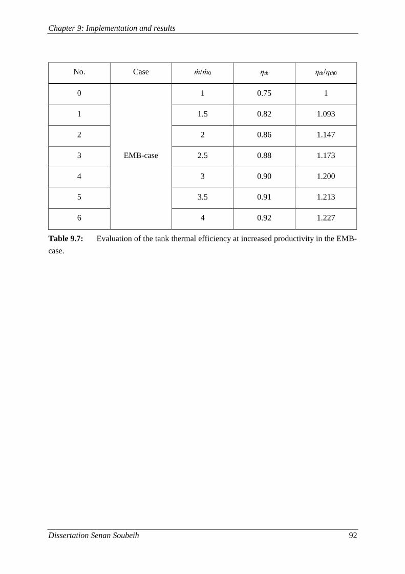
Chapter 9: Implementation and results
Dissertation Senan Soubeih 92
No. Case ṁ/ṁ0 ηth ηth/ηth0
0
EMB-case
1 0.75 1
1 1.5 0.82 1.093
2 2 0.86 1.147
3 2.5 0.88 1.173
4 3 0.90 1.200
5 3.5 0.91 1.213
6 4 0.92 1.227
Table 9.7: Evaluation of the tank thermal efficiency at increased productivity in the EMB-
case.
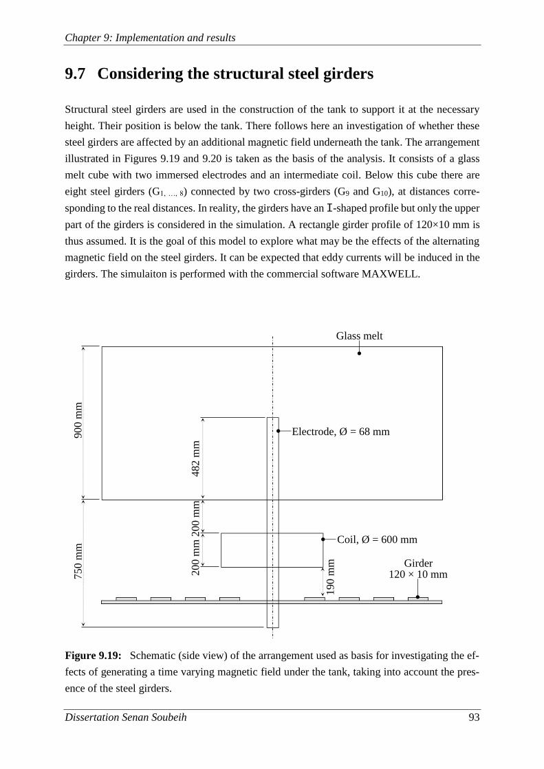
Chapter 9: Implementation and results
Dissertation Senan Soubeih 93
9.7 Considering the structural steel girders
Structural steel girders are used in the construction of the tank to support it at the necessary
height. Their position is below the tank. There follows here an investigation of whether these
steel girders are affected by an additional magnetic field underneath the tank. The arrangement
illustrated in Figures 9.19 and 9.20 is taken as the basis of the analysis. It consists of a glass
melt cube with two immersed electrodes and an intermediate coil. Below this cube there are
eight steel girders (G1, …, 8) connected by two cross-girders (G9 and G10), at distances corre-
sponding to the real distances. In reality, the girders have an I-shaped profile but only the upper
part of the girders is considered in the simulation. A rectangle girder profile of 120×10 mm is
thus assumed. It is the goal of this model to explore what may be the effects of the alternating
magnetic field on the steel girders. It can be expected that eddy currents will be induced in the
girders. The simulaiton is performed with the commercial software MAXWELL.
Figure 9.19: Schematic (side view) of the arrangement used as basis for investigating the ef-
fects of generating a time varying magnetic field under the tank, taking into account the pres-
ence of the steel girders.
900 m
m
750 m
m
482 m
m
200 m
m
200 m
m
19
0 m
m
120 × 10 mm
Glass melt
Electrode, Ø = 68 mm
Coil, Ø = 600 mm
Girder
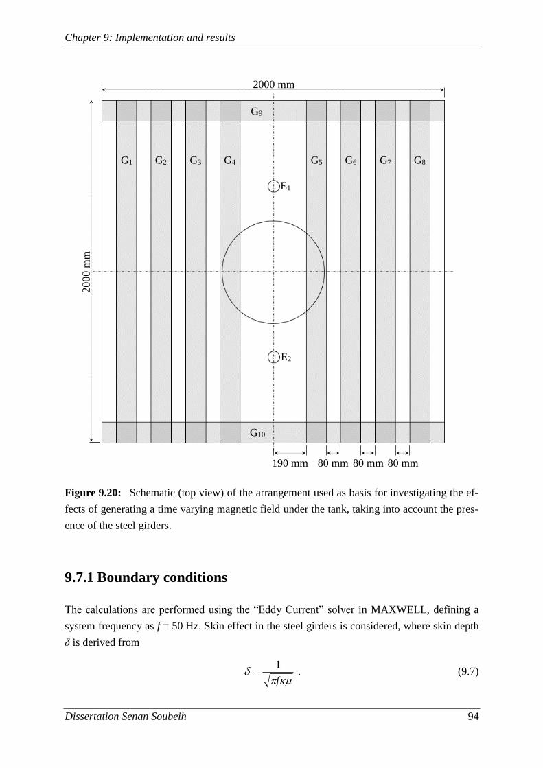
Chapter 9: Implementation and results
Dissertation Senan Soubeih 94
9.7.1 Boundary conditions
The calculations are performed using the “Eddy Current” solver in MAXWELL, defining a
system frequency as f = 50 Hz. Skin effect in the steel girders is considered, where skin depth
δ is derived from
f
1 . (9.7)
Figure 9.20: Schematic (top view) of the arrangement used as basis for investigating the ef-
fects of generating a time varying magnetic field under the tank, taking into account the pres-
ence of the steel girders.
2000 mm 2000 m
m
190 mm 80 mm 80 mm 80 mm
G1 G2 G3 G4 G5 G6 G7 G8
G9
G10
E2
E1
Chapter 9: Implementation and results
Dissertation Senan Soubeih 95
κ and μ are respectively the electrical conductivity and magnetic permeability of the steel gird-
ers. The simulation assumes κ = 7142857 S/m and a simplified relative magnetic permeability
μr = 1000. With these assumptions δ = 0.842169 mm. These material properties are typical of
the S235JR type of structural steel which is usually used in the construction of glass-melting
furnaces. To enhance the accuracy of the calculation, the case-characteristic skin depth
δ = 0.842169 mm is used to define a “Skin Depth Based” adaptive mesh refinement in MAX-
WELL, to be applied to the upper surface of the girders.
The coil is modeled as a single object made of copper conductor material, with a terminal in
the cross section. On the terminal, the current source applied is a “Stranded” alternating current
source with a peak value of 204252 A (assuming the effective value IC = 425 A of the
EMB-case). With the Stranded boundary condition, the electric current density will be uni-
formly distributed over the coil terminal. A coil with 20 turns and a peak electric current of
4252 A through each turn is thus represented. At the bottom surface of the electrodes, a
current source with a peak value of 5.23042 A is defined. The electrode current is assumed
to be entering through the bottom surface of the electrode E1 and exiting from that of the elec-
trode E2. The magnetic field of the coil and the eigenfield of the electrodes are added together,
forming the total magnetic field. Additionally, a region of ambient air is defined with a padding
percentage of 200%. For the magnetic field, “Neumann” boundary condition is assumed on all
outer boundaries. Under this condition, the magnetic field is tangential to the boundary and
cannot cross it. The Neumann boundary condition corresponds to symmetry conditions and is
set by default in MAXWELL. On the interfaces between objects, the natural boundary condition
is assumed for the magnetic field, which means that the normal component of the magnetic
field is continuous across the interface boundaries.
9.7.2 Results and discussion
Figure 9.21 demonstrates the electric current density induced in the girder G4, in which the
largest eddy current intensity exists. The figure represents the electric current density in a cross
sectional plane through the centre of G4. Eddy currents have the largest density of about
8×10⁵ A/m² in the region of the upper surface of the girder. However, the greater the distance
between a girder and the coil, the less intense the eddy current induced. The ohmic loss density
is shown in Figure 9.22 for the same cross sectional plane of G4. Again, the largest ohmic loss
exists in the region of the upper surface of the girder with a density of about 1.5×10⁵ W/m³. In
addition to the eddy currents, sinusoidal short-circuit currents flow through the connected gird-
ers. The maximum currents flow through G9 and G10. The peak values of the short-circuit cur-
rents flowing through the girders are presented in Table 9.8.
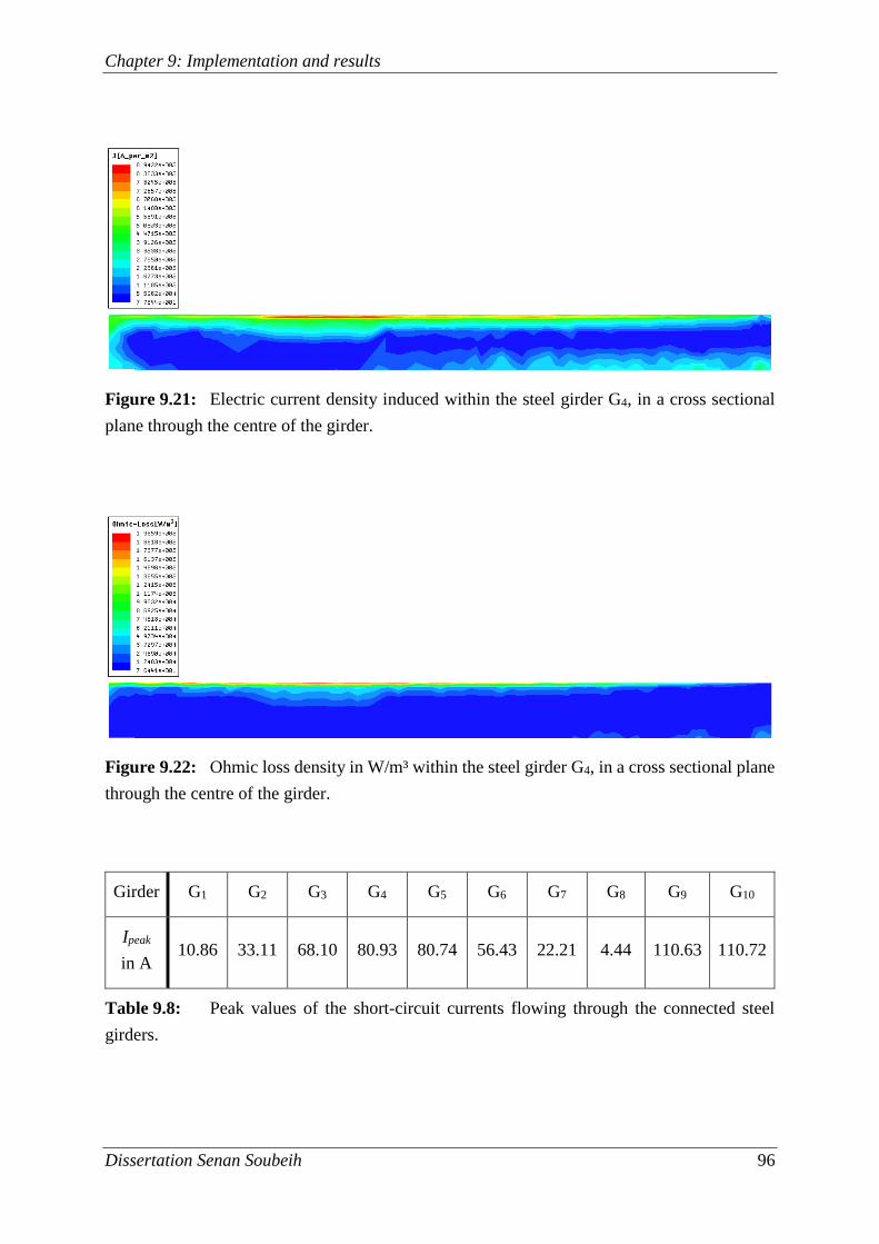
Chapter 9: Implementation and results
Dissertation Senan Soubeih 96
Figure 9.21: Electric current density induced within the steel girder G4, in a cross sectional
plane through the centre of the girder.
Figure 9.22: Ohmic loss density in W/m³ within the steel girder G4, in a cross sectional plane
through the centre of the girder.
Girder G1 G2 G3 G4 G5 G6 G7 G8 G9 G10
Ipeak
in A 10.86 33.11 68.10 80.93 80.74 56.43 22.21 4.44 110.63 110.72
Table 9.8: Peak values of the short-circuit currents flowing through the connected steel
girders.
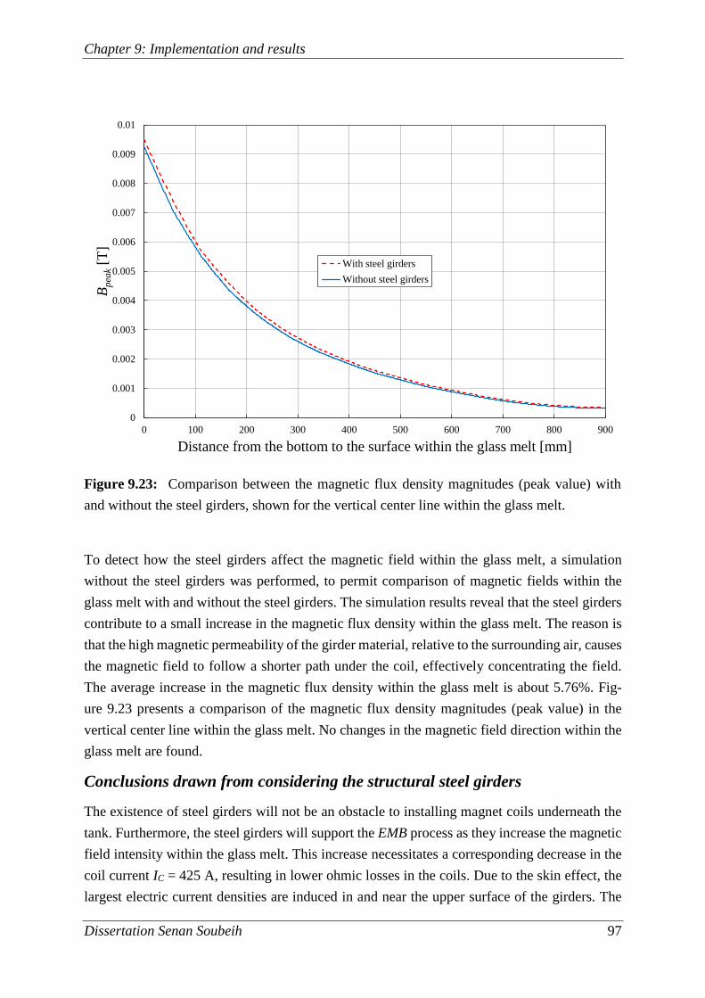
Chapter 9: Implementation and results
Dissertation Senan Soubeih 97
To detect how the steel girders affect the magnetic field within the glass melt, a simulation
without the steel girders was performed, to permit comparison of magnetic fields within the
glass melt with and without the steel girders. The simulation results reveal that the steel girders
contribute to a small increase in the magnetic flux density within the glass melt. The reason is
that the high magnetic permeability of the girder material, relative to the surrounding air, causes
the magnetic field to follow a shorter path under the coil, effectively concentrating the field.
The average increase in the magnetic flux density within the glass melt is about 5.76%. Fig-
ure 9.23 presents a comparison of the magnetic flux density magnitudes (peak value) in the
vertical center line within the glass melt. No changes in the magnetic field direction within the
glass melt are found.
Conclusions drawn from considering the structural steel girders
The existence of steel girders will not be an obstacle to installing magnet coils underneath the
tank. Furthermore, the steel girders will support the EMB process as they increase the magnetic
field intensity within the glass melt. This increase necessitates a corresponding decrease in the
coil current IC = 425 A, resulting in lower ohmic losses in the coils. Due to the skin effect, the
largest electric current densities are induced in and near the upper surface of the girders. The
Figure 9.23: Comparison between the magnetic flux density magnitudes (peak value) with
and without the steel girders, shown for the vertical center line within the glass melt.
0
0.001
0.002
0.003
0.004
0.005
0.006
0.007
0.008
0.009
0.01
0 100 200 300 400 500 600 700 800 900
Bp
eak
[T]
Distance from the bottom to the surface within the glass melt [mm]
With steel girders
Without steel girders
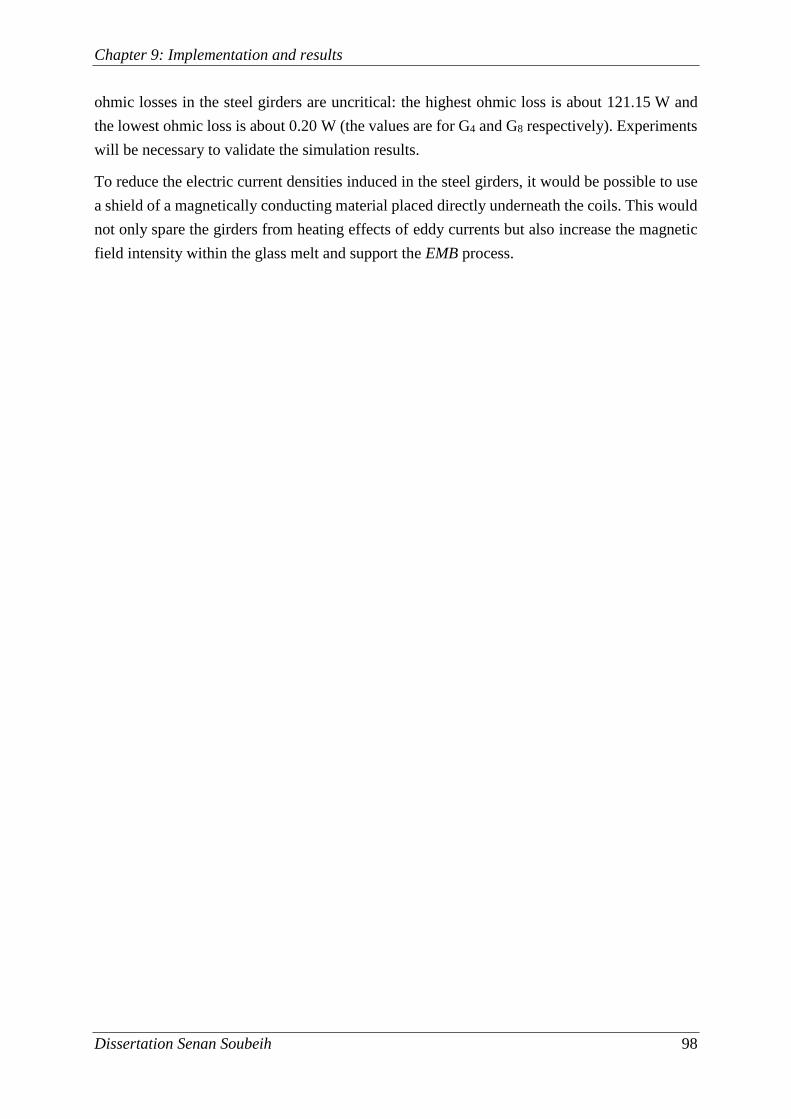
Chapter 9: Implementation and results
Dissertation Senan Soubeih 98
ohmic losses in the steel girders are uncritical: the highest ohmic loss is about 121.15 W and
the lowest ohmic loss is about 0.20 W (the values are for G4 and G8 respectively). Experiments
will be necessary to validate the simulation results.
To reduce the electric current densities induced in the steel girders, it would be possible to use
a shield of a magnetically conducting material placed directly underneath the coils. This would
not only spare the girders from heating effects of eddy currents but also increase the magnetic
field intensity within the glass melt and support the EMB process.
Chapter 10: Conclusion and outlook
Dissertation Senan Soubeih 99
10 Conclusion and outlook
10.1 Conclusion
This thesis has reported numerical simulations which explore how Lorentz forces generated
additionally to the conventional forces in an electrically boosted continuous glass-melting tank
can improve the RTD. The additional Lorentz forces come in this case from an externally gen-
erated magnetic field interacting with the electric currents that are flowing through the glass
melt. For this purpose, additional magnet coils are placed underneath the tank bottom and po-
sitioned between the boosting electrodes. The additional Lorentz forces are orientated against
the main direction of flow within the tank, with the effect of preventing the colder, less well-
melted bottom glass from flowing between the electrodes directly to the tank-outlet. This bot-
tom glass thus has a longer residence time within the tank. The new and innovative approach is
called electromagnetic boosting, EMB. The work represents the first investigation of the em-
ployment of additionally generated Lorentz forces to improve the performance of an industrial
continuous glass-melting tank.
Because of the temperature-dependent physical properties of glass, coupled electrodynamic,
thermodynamic, and hydrodynamic effects have to be calculated for the numerical simulation.
Coupling of the calculations is achieved by implementing electromagnetic field calculation in
the commercial software program FLUENT (developed for calculating coupled hydrodynamic
and thermodynamic effects on the basis of FVM). This coupling method has been tested, and
the electromagnetic field calculation with FLUENT has been validated by numerical simulation
using the commercial software MAXWELL (developed for calculating electromagnetic effects
on the basis of FEM). The author has found the method to be reliable and accurate.
The simulations have been performed for an actual industrial-scale continuous glass-melting
tank using an academic representation of the tank. The goal was a model permitting investiga-
tion of the pure effects of the additionally generated Lorentz forces on the flow pattern within
the tank and basic evaluation of the EMB. The boundary conditions were so defined as to sim-
ulate the realistic conditions in the actual tank. The numerical simulations were thoroughly
verified to ensure sufficient numerical accuracy. The simulation results were found to agree
qualitatively with the expected characteristics of the industrial continuous glass-melting tank.
An external magnet coils system was adapted to realize EMB in the tank considered. The sim-
ulations showed that it is basically possible to create an electromagnetic wall within the glass
melt between the boosting electrodes. Further parameter analyses were carried out to establish
the optimum EMB effects, which are optimally increased MRT and improved RTD. With the
simulation, it was possible for the first time to predict and analyze the dynamic behavior of
Chapter 10: Conclusion and outlook
Dissertation Senan Soubeih 100
operating electromagnetically boosted continuous glass-melting tank. This dynamic operation
was analyzed for the case both with and without EMB. The comparison revealed that EMB is
favorably affecting the glass melt flow within the tank, increasing the MRT substantially and
thus enhancing the glass quality. RTD in the tank was also improved, which, in turn, resulted
in more homogeneous timed distribution of the energy consumed. Moreover, with EMB, the
tank simulations showed that it is possible to simultaneously increase the tank productivity and
enhance the glass quality. This is not possible in the ordinary tank operation case without EMB.
The rise in tank productivity leads to higher tank thermal efficiency. As an ultimate result, the
tank performance has been substantially enhanced by EMB.
10.2 Outlook
In this work, the calculations have been coupled by a numerical method which is an efficient
means of addressing Multiphysics problems. The method can be extended to a wide range of
coupled problems. It would be possible to include eddy currents and the currents induced by
movement of conducting bodies in future simulations.
The new innovative concept of EMB to provide a contactless flow control in continuous glass-
melting tanks can be further supported by plates of a magnetically conducting material to in-
crease the magnetic field intensity within the glass melt. Such plates would mean that ohmic
losses in the coils could be reduced by decreasing the currents in them, but would involve ad-
ditional costs.
Installing an EMB system is viable investment which will improve the operational flexibility of
continuous glass-melting tanks. The present work is the foundation necessary to convert the
idea into an effective industrial process in the future. The results have already been discussed
at specialized conferences of the glass industry and found to be promising. However, no indus-
trial partner is yet ready to embark on a costly and large construction with risky conditions so
that the process is performed on an operating tank. The first step, always the most important,
has been taken en route to a sophisticated glass-melting tank characterized by high efficiency
and high production quality. Using EMB to improve the tank efficiency and increase the pro-
duction quality simultaneously will serve the constant aim of glass manufacturing, which is to
produce high quality glass as cheaply as possible. The range of application of the technique
could also be extended to different tank types and sizes, enabling a variety of goals to be met,
among them a substantial reduction in energy consumed.
Bibliography
Dissertation Senan Soubeih 101
Bibliography
[1] P. McCray (Ed.), The prehistory & history of glassmaking technology: [proceedings of
the Prehistory and History of Glassmaking Technology Symposium, held at the 99th An-
nual Meeting of the American Ceramic Society in Cincinnati, Ohio, May 4 - 7, 1997],
American Ceramic Soc, Westerville, Ohio, 1998.
[2] W.S. Ellis, Glass: From the first mirror to fiber optics, the story of the substance that
changed the world, 1st ed., Avon Books, New York, c1998.
[3] S.C. Rasmussen, How glass changed the world: The history and chemistry of glass from
antiquity to the 13th century, Springer, Heidelberg, 2012.
[4] H.G. Pfaender, Schott guide to glass, 2nd ed., Chapman & Hall, London, 1996.
[5] S. Spauszus, D. Schnapp, Glas allgemeinverständlich: Eine Einführung in Theorie und
Praxis, 1st ed., VEB Fachbuchverlag, Leipzig, 1977.
[6] I. Fanderlik (Ed.), Silica glass and its application, Elsevier, Amsterdam, 1991.
[7] H. Rawson, Properties and applications of glass, 1st ed., Elsevier, Amsterdam, 1984.
[8] C.W. Sinton, Raw materials for glass and ceramics: Sources, processes, and quality con-
trol, Wiley, Hoboken, NJ, 2006.
[9] J. Lange, Rohstoffe der Glasindustrie ; mit 128 Tabellen, 3rd ed., Dt. Verl. für Grund-
stoffindustrie, Leipzig, 1993.
[10] T.H. Finger, Glass Batch Plant Control with Small Computers, IEEE Trans. on Ind. Ap-
plicat. IA-8 (1972) 168–172.
[11] J.E. Polcyn, W.C. Susor, Computer Controlled Glass Batching System, IEEE Trans. on
Ind. Applicat. IA-8 (1972) 542–548.
[12] P.J. Doyle, Glass-making today: An introduction to current practice in glass manufacture,
Portcullis Press; Available from International Publications Service, Collins, Redhill
[England], New York, 1979.
[13] G. Nölle, Technik der Glasherstellung: 41 Tabellen, 3rd ed., Dt. Verl. für Grund-
stoffindustrie, Stuttgart, 1997.
[14] F.V. Tooley, The Handbook of glass manufacture: a book of reference for the plant exec-
utive, technologist and engineer, Books for Industry Inc., New York, 1974.
[15] W. Trier, Glasschmelzöfen: Konstruktion und Betriebsverhalten ; mit 63 Tabellen, Sprin-
ger, Berlin, 1984.
Bibliography
Dissertation Senan Soubeih 102
[16] O. Verworner, K. Berndt, Feuerfeste Baustoffe für Glasschmelzanlagen: Feuerfeste Bau-
stoffe ; Glasschmelzanlagen ; Bauelemente der Glasschmelzanlagen, ihre Baustoffe und
Beanspruchung ; mit 112 Bildern, 49 Tabellen, 1st ed., Dt. Verl. für Grundstoffindustrie,
Leipzig, 1978.
[17] G.A. Pecoraro, J.C. Marra, J.T. Wenzel (Eds.), Corrosion of materials by molten glass,
American Ceramic Society, Westerville, Ohio, 1996.
[18] O. Levenspiel, Chemical reaction engineering, 3rd ed., Wiley, Hoboken, NJ, 1999.
[19] H. Bach, Baucke, Friedrich G. K., D. Krause, Electrochemistry of glasses and glass
melts, including glass electrodes: With 22 tables, Springer, Berlin, 2001.
[20] S.K. Sundaram (Ed.), Electrochemistry of glass and ceramics: [proceedings of the Elec-
trochemistry of Glass and Ceramics Symposium, held at the 100th annual meeting of the
American Ceramic Society in Cincinnati, Ohio, May 3 - 6, 1998], American Ceramic So-
ciety, Westerville, Ohio, 1999.
[21] R.H. Doremus, Glass science, 2nd ed., Wiley, New York, NY, 1994.
[22] Nikolaus Sorg GmbH & Co KG, Glass Melting Technology. GlasE/10.08/V2.2.
[23] R. Kessel, R. Sims, Die elektrische Zusatzbeheizung für Schmelzwannen - Technologie-
stand 2005, in: Proceedings 79. Glasstechnische Tagung, Würzburg, 2005.
[24] R.D. Argent, Modern trends in electrode utilization, IEEE Trans. on Ind. Applicat. 26
(1990) 175–182.
[25] J.S. Stroud, Molybdenum Electrodes in Glass Tanks, IEEE Trans. on Ind. Applicat. IA-
13 (1977) 618–625.
[26] IEEE Institute of Electrical and Electronics Engineers, Inc, IEEE Recommended Pratice
for Electrical Heating Applications to Melting Furnaces and Forehearths in the Glass In-
dustry, IEEE, New York, 1986.
[27] U. Lüdtke, S. Soubeih, B. Halbedel, U. Krieger, A. Kelm, Numerische Simulation der
Strömung einer Glasschmelze unter dem Einfluss von extern generierten Lorentzkräften,
in: Tagungsband Workshop Elektroprozesstechnik, Heyda, Germany, 2011.
[28] U. Lüdtke, S. Soubeih, B. Halbedel, Numerische Simulation der Strömung in einer Glas-
wanne mit Barriere-Boostelektroden unter dem Einfluss von extern generierten Lorentz-
kräften, in: Tagungsband Workshop Elektroprozesstechnik, Heyda, Germany, 2012.
[29] U. Luedtke, S. Soubeih, B. Halbedel, Numerical simulation of induced alterations of flow
patterns within glass melts using external Lorentz forces, Journal of iron and steel re-
search international 19 (2012) 471–474.
Bibliography
Dissertation Senan Soubeih 103
[30] U. Luedtke, S. Soubeih, B. Halbedel, Numerical simulation of electromagnetically con-
trolled flow in glass melting tanks, in: Proceedings of the International Conference on
Heating by Electromagnetic Sources HES-13, Padua, Italy, 2013, pp. 45–52.
[31] U. Lüdtke, S. Soubeih, B. Halbedel, Numerische Simulation von Glaswannen mit Barrie-
rebooster unter dem Einfluss von extern generierten Lorentzkräften - Vergleich verschie-
dener Spulensysteme, in: Tagungsband Workshop Elektroprozesstechnik, Heyda, Ger-
many, 2013.
[32] B. Halbedel, J.O. Torres, U. Lüdtke, S. Soubeih, Nutzung von Lorentzkräften in der
Glasschmelztechnik, in: Thüringer Werkstofftag 2013, Ilmenau, Germany, 2013, pp. 25–
32.
[33] S. Soubeih, U. Lüdtke, B. Halbedel, Numerical simulation and optimization of a glass
melting tank with magnet coil system to improve the residence time distribution, in: Ta-
gungsband Workshop Elektroprozesstechnik, Heyda, Germany, 2014.
[34] U. Lüdtke, S. Soubeih, B. Halbedel, Using Numerical Simulation to Optimize the Exter-
nal Magnet System Needed to Improve the Residence Time Distribution of Glass Melt-
ing Tanks, in: Proceedings of the International Scientific Colloquium Modelling for Elec-
tromagnetic Processing, Hannover, Germany, 2014, pp. 177–182.
[35] S. Soubeih, U. Luedtke, B. Halbedel, Improving Residence Time Distribution in Glass
Melting Tanks Using Additionally Generated Lorentz Forces, J. Chem. Chem. Eng. 9
(2015) 203–210.
[36] S. Soubeih, U. Luedtke, B. Halbedel, Numerical simulation of electromagnetically con-
trolled flow in glass melting process, in: Proceedings of the 23rd International Congress
on Glass, Prague, Czech Republic, 2013.
[37] S. Soubeih, U. Luedtke, B. Halbedel, Using numerical simulation to study the effects of
how an external magnet system improves the residence time distribution on glass melting
tanks, in: Proceedings of the 1st Joint Meeting of DGG – ACerS GOMD, Aachen, Ger-
many, 2014.
[38] S. Soubeih, U. Luedtke, B. Halbedel, Numerical simulation of a glass melting tank with a
magnet system to improve the residence time distribution, in: Proceedings of the 12th
ESG Conference, Parma, Italy, 2014.
[39] S. Soubeih, U. Lüdtke, B. Halbedel, Using Numerical Simulation to Investigate How Ad-
ditional Lorentz Forces Improve the Residence Time Distribution in Industrial Glass
Melting Tanks, in: Proceedings of the ANSYS Conference & 33. CADFEM Users' Meet-
ing, Bremen, Germany, 2015, pp. 2.7.6.
Bibliography
Dissertation Senan Soubeih 104
[40] R.A. Murnane, D.A. Nolet, Evolution of simulation techniques to model electric glass
furnaces, in: Conference Record of the IEEE Industry Applications Society Annual
Meeting, San Diego, CA, USA, 1-5 Oct. 1989, pp. 1384–1394.
[41] H. De Waal, Mathematical modeling of the glass melting process, Glastech. Ber. 63K
(1990) 1–18.
[42] S.R. Venkateswaran, J.L. Conrad, G.A. Walzer, Modeling of the glass melting process,
in: Conference Record of the 1990 IEEE Industry Applications Society Annual Meeting,
Seattle, WA, USA, 7-12 Oct. 1990, pp. 1343–1348.
[43] M.K. Choudhary, N.T. Huff, Mathematical modeling in the glass industry: An overview
of status and needs, Glastech. Ber. Glass Sci. Technol. 70 (1997) 363–370.
[44] H. Loch, D. Krause (Eds.), Mathematical simulation in glass technology: With 17 tables
and 27 videos on CD, Springer, Berlin, 2002.
[45] R.L. Curran, Use of Mathematical Modeling in Determining the Effects of Electrode
Configuration on Convection Currents in an Electric Glass Melter, IEEE Trans. on Ind.
Gen. Applicat. IGA-7 (1971) 116–129.
[46] R.L. Curran, Mathematical Model of an Electric Glass Furnace: Effects of Glass Color
and Resistivity, IEEE Trans. on Ind. Applicat. IA-9 (1973) 348–357.
[47] M.J. Austin, D.E. Bourne, A mathematical model of an electric glass furnace, Glass
Technology 14 (1973) 78–84.
[48] G. Leyens, Beitrag zur Berechnung zweidimensionaler Konvektionsströmungen in konti-
nuierlich betriebenen Glasschmelzwannen: Teil 1. Mathematisches Modell. Teil 2. Er-
gebnisse der Berechnungen, Glastech. Ber. 47 (1974) 251-259 & 261-270.
[49] H. Mase, K. Oda, Mathematical model of glass tank furnace with batch melting process,
Journal of Non-Crystalline Solids 38 & 39 (1980) 807–812.
[50] L. Mardorf, G. Woelk, Berechnung des Verhaltens einer elektrisch beheizten Glas-
schmelzwanne mit einem mathematischen Modell, Glastech. Ber. 56 (1983) 73–84.
[51] G. Leyens, J. Smrček, Einfluß der Badtiefe und des Durchsatzes auf die Strömungen in
der Glasschmelzwanne, Glastech. Ber. 55 (1982) 81–87.
[52] G. Leyens, J. Smrček, J. Thyn, Anwendung der Isotopen-Meßtechnik und eines mathe-
matischen Modells zur Bestimmung der Strömungsverteilung in einer Schmelzwanne,
Glastech. Ber. 53 (1980) 124–129.
[53] D.A. Nolet, Applications of modeling and process analysis to furnace operations and re-
design, in: Proceedings of the 46th Conference on Glass Problems, Urbana, USA, 1985,
pp. 329–339.
Bibliography
Dissertation Senan Soubeih 105
[54] T.-S. Chen, R.E. Goodson, Computation of three-dimensional temperature and convec-
tive flow profiles for an electric glass furnace, Glass Technology 13 (1972).
[55] A. Moult, Two and three dimensional mathematical models of glass tank furnaces, Glass
Technology 23 (1982) 106–112.
[56] F. Simonis, H. De Waal, R.C.G. Beerkens, Influence of furnace design and operation pa-
rameters on the residence time distribution of glass tanks, predicted by 3-D computer
simulation, in: Collected papers, XIV International Congress on Glass, Calcutta, 1986,
pp. 118–127.
[57] A. Ungan, R. Viskanta, Three-Dimensional Numerical Simulation of Circulation and
Heat Transfer in an Electrically Boosted Glass Melting Tank, IEEE Trans. on Ind. Ap-
plicat. IA-22 (1986) 922–933.
[58] A. Ungan, R. Viskanta, Three-dimensional numerical modeling of circulation and heat
transfer in a glass melting tank: Part 1. Mathematical formulation. Part 2. Sample simula-
tions, Glastech. Ber. 60 (1987).
[59] M.K. Choudhary, A Three-Dimensional Mathematical Model for Flow and Heat Transfer
in Electrical Glass Furnaces, IEEE Trans. on Ind. Applicat. IA-22 (1986) 912–921.
[60] M.K. Choudhary, A modeling study of flow and heat transfer in an electric melter, Jour-
nal of Non-Crystalline Solids 101 (1988) 41–53.
[61] A.A. Ghandakly, R.L. Curran, Accurate modeling of interelectrode resistance and power
dissipation in electric glass melters, IEEE Trans. on Ind. Applicat. 24 (1988) 1057–1061.
[62] R.A. Murnane, W.W. Johnson, N.J. Moreland, The analysis of glass melting processes
using three-dimensional finite elements, International Journal for Numerical Methods in
Fluids 8 (1988) 1491–1511.
[63] M.G. Carvalho, M. Nogueira, Modelling of glass melting industrial process, JOURNAL
DE PHYSIQUE IV 3/C7 (1993) 1357–1366.
[64] R.G.C. Beerkens, T. van der Heijden, E. Muijsenberg, Possibilities of glass tank model-
ing for the prediction of the quality of melting processes, Ceram. Eng. Sci. Proc. 14(3-4)
(1993) 139–160.
[65] R. Beerkens, Heutige Möglichkeiten zur Modellierung von Glasschmelzöfen voraussa-
gen zur Qualität des Glasschmelzprozesses, Glastech. Ber. Glass Sci. Technol. 71 (1998).
[66] K.O. Lim, T.H. Song, K.S. Lee, Patterns of natural convection driven by the free surface
temperature distribution in a glass melting furnace, Glass Technology 39 (1998) 27–31.
Bibliography
Dissertation Senan Soubeih 106
[67] L. Pilon, G. Zhao, R. Viskanta, Three-dimensional flow and thermal structures in glass
melting furnaces: Part I. effects of the heat flux distribution. Part II. effects of batch blan-
ket and bubbles, Glass Sci. Technol. 75 (2002) 55–68 & 115-124.
[68] T. Hiejima, H. Azuma, M. Sawasaki, Numerical analysis and measurement of glass flow
in a small melting furnace, Glass Sci. Technol. 76 (2003) 155–165.
[69] V. Sardeshpande, U.N. Gaitonde, R. Banerjee, Model based energy benchmarking for
glass furnace, Energy Conversion and Management 48 (2007) 2718–2738.
[70] S. Gopalakrishnan, A. Thess, G. Weidmann, U. Lange, Chaotic mixing in a Joule-heated
glass melt, Phys. Fluids 22 (2010) 013101.
[71] W. Muschick, E. Muysenberg, Round robin for glass tank models: Report of the Interna-
tional Commission on Glass (ICG) Technical Committee 21 "Modeling of Glass Melts",
Glastech. Ber. Glass Sci. Technol. 71 (1998) 153–156.
[72] C. Moukarzel, W.S. Kuhn, D. Clodic, Numerical precision of minimum residence time
calculations for glass tanks: Recalculation of Round Robin Test 1 of Technical Commit-
tee 21 "Modelling of Glass Melts" of the International Commission on Glass (ICG),
Glass Sci. Technol. 76 (2003).
[73] R. Beerkens, Analysis of elementary process steps in industrial glass melting tanks -
Some ideas on innovations in industrial glass melting, Ceramics − Silikáty 52 (2008)
206–217.
[74] H.P.H. Muysenberg, F. Simonis, Verification of 3D mathematical simulation with meas-
ured temperature profiles during furnace operation, Glastech. Ber. Glass Sci. Technol.
68C2 (1995) 55–62.
[75] J. Bauer, U. Roger, P. Simons, Validation of a mathematical glass tank model, Glastech.
Ber. Glass Sci. Technol. 72 (1999) 171–181.
[76] E. Muysenberg, M. Nováčková, M. Trochta, P. Viktorin, Advanced melter operation and
training tool, Glass Sci. Technol. 75 (2002) 209–215.
[77] O.R. Hofmann, H. Kaliski, Die elektromagnetische Kraftwirkung auf die Glasschmelze
in Elektrodennähe, Silikattechnik 42 (1991) 19–21.
[78] O.R. Hofmann, G. Philipp, Importance of the Lorentz force in electrically heated glass
melts, Glastech. Ber. 65 (1992) 142–149.
[79] G. Philipp, O.R. Hofmann, Modelling of electrically heated glass melting furnaces needs
inclusion of Lorentz force, in: Fundamentals of glass science and technology 1993: Pro-
ceedings of the Second Conference of the European Society of Glass Science and Tech-
nology, Venice, Italy, 1993, pp. 235–240.
Bibliography
Dissertation Senan Soubeih 107
[80] M.K. Choudhary, Mathematical modeling of MHD and buoyancy driven flow in electric
furnaces, in: Proceedings II International Seminar on Mathematical Simulation in the
Glass Melting, Vsetin, Czech Republic, 1993, pp. 87–98.
[81] M.K. Choudhary, A modeling study of flow and heat transfer in the vicinity of an elec-
trode, in: Proceedings of the XVII International Congress on Glass, Beijing, China, 1995,
pp. 100–107.
[82] O.R. Hofmann, A. Thess, Elektromagnetische Beeinflussung der Glasbadströmung - ein
neues Anwendungsgebiet der Magnetohydrodynamik, Glas-Ingenieur 1 (2002) 39–45.
[83] O.R. Hofmann, Electromagnetic force in electric glass melting, Glass Sci. Technol. 76
(2003).
[84] L.G. Bates, F.E. Haskell US1853843, 1932.
[85] A.J. Walkden GB1289317, 1972.
[86] A.E. Mikelson, V.N. Moshnyaga, A.D. Osmanis, V.T. Slavyanskij, V.S. Shashkin
SU814904, 1981.
[87] A.D. Osmanis, A.E. Mikelson, L.Y. Pochs, I. Barbans, O.M. Mezhdrejs, V.V. Troshin,
V.I. Butaeva, N.M. Vygorka, A.I. Grigorev, V.M. Zalevskij SU1024423A.
[88] V.N. Fekolin, F.A. Stupak, The application of the magnetohydrodynamic effect to the ag-
itation of glass, Glass Ceram 41 (1984) 531–535.
[89] C. Kunert, A. Langsdorf, F.T. Lentes, K.D. Duch, A. Thess, Y. Kolesnikow
DE102004015055A1, 2005.
[90] C. Giessler, U. Lange, A. Thess, Nonlinear laminar pipe flow of fluids with strongly tem-
perature-dependent material properties, Phys. Fluids 19 (2007) 043601.
[91] C. Giessler, R. Schlegel, A. Thess, Numerical investigation of the flow of a glass melt
through a long circular pipe, International Journal of Heat and Fluid Flow 29 (2008)
1462–1468.
[92] C. Gießler, Theoretical investigations of electromagnetic control of glass melt flow. Dis-
sertation, Technische Universität Ilmenau, 2008.
[93] D. Hülsenberg, B. Halbedel, G. Conrad, A. Thess, Y. Kolesnikov, U. Lüdtke, Electro-
magnetic stirring of glass melts using Lorentz forces - Experimental results, Glass Sci.
Technol. 77 (2004) 186–193.
[94] U. Krieger, Einfluss elektromagnetisch generierter Kraftwirkungen auf die Strömung in
Glasschmelzen. Dissertation, Technische Universität Ilmenau, 2007.
[95] U. Krieger, B. Halbedel, D. Hülsenberg, A. Thess, Electromagnetic effects on glass melt
flow in crucibles, Glass Technol.: Eur. J. Glass Sci. Technol. A 49 (2008) 33–40.
Bibliography
Dissertation Senan Soubeih 108
[96] D. Cepite, A. Jakovičs, B. Halbedel, U. Krieger, Modelling of electromagnetic glass con-
vection with temperature-dependent properties of the melt, Magnetohydrodynamics 43
(2007) 195–204.
[97] C. Giessler, C. Sievert, U. Krieger, B. Halbedel, D. Huelsenberg, U. Luedtke, A. Thess,
A model for electromagnetic control of buoyancy driven convection in glass melts,
FDMP 1 (2005) 247–266.
[98] C. Giessler, A. Thess, Electromagnetic control of thermal convection of a fluid with
strongly temperature-dependent material properties, J. Fluid Mech. 618 (2009) 135–154.
[99] C. Giessler, A. Thess, Numerical simulation of electromagnetically controlled thermal
convection of glass melt in a crucible, International Journal of Heat and Mass Transfer
52 (2009) 3373–3389.
[100] B. Halbedel, D. Hülsenberg, U. Krieger, U. Lüdtke, G. Carl, H.-J. Linz
DE102005058729A1, 2007.
[101] O.R. Hofmann DE102008011008A1, 2009.
[102] S. Gopalakrishnan, A. Thess, Electromagnetically induced chaotic mixing in a pipe
mixer, Chemical Engineering Science 65 (2010) 6282–6291.
[103] J.O. Torres, B. Halbedel, A novel electromagnetic mixer for the glass melt homogeni-
zation - evaluation with a numerical and physical model, in: Tagungsband Workshop
Elektroprozesstechnik, Heyda, Germany, 2012.
[104] A.P. Kelm, Numerische Simulation der Strömungsbeeinflussung einer Glasschmelze
mit Hilfe von Lorentzkräften. Diplomarbeit, Technische Universität Ilmenau, 2010.
[105] J.O. Torres, B. Halbedel, C. Weber, R. Reche, High-performance forehearth coloring
using Lorentz forces, in: Tagungsband Workshop Elektroprozesstechnik, Heyda, Ger-
many, 2014.
[106] HVG and DGG, Standardglas I der DGG (Kalk-Natron-Glas), available at
http://www.hvg-dgg.de/fileadmin/dateien/verein/Standardglas_Ia.pdf (2012).
[107] H. Loch, Overview, in: H. Loch, D. Krause (Eds.), Mathematical simulation in glass
technology: With 17 tables and 27 videos on CD, Springer, Berlin, 2002, pp. 1–15.
[108] B. Halbedel, Messberichte (unpublished document). Technische Universität Ilmenau,
Fachgebiet Anorganisch-nichtmetallische Werkstoffe, Ilmenau, 2012.
[109] R.G. Beerkens, Modeling of the melting process in industrial glass furnaces, in: H.
Loch, D. Krause (Eds.), Mathematical simulation in glass technology: With 17 tables
and 27 videos on CD, Springer, Berlin, 2002, pp. 17–73.
[110] J.D. Jackson, Classical electrodynamics, 3rd ed., Wiley, New York, NY, c 1999.
Bibliography
Dissertation Senan Soubeih 109
[111] R.J. Moreau, Magnetohydrodynamics, Kluwer, Dordrecht, 1990.
[112] F.-T. Lentes, High-frequency melting of glass in crucibles, in: H. Loch, D. Krause
(Eds.), Mathematical simulation in glass technology: With 17 tables and 27 videos on
CD, Springer, Berlin, 2002, pp. 126–155.
[113] W.M. Rohsenow (Ed.), Handbook of heat transfer, 3rd ed., McGraw-Hill, New York,
NY, 1998.
[114] G. Nellis, S. Klein, Heat transfer, Cambridge Univ. Press, Cambridge, 2009.
[115] U. Lüdtke, Numerische Simulation gekoppelter Felder in der Elektroprozesstechnik.
Habilitationsschrift, Technische Universität Ilmenau, 2014.
[116] ANSYS FLUENT: Help, ANSYS Inc., 2014.
[117] N. Ida, Engineering electromagnetics, Springer, New York, 2000.
[118] P.J. Roache, Verification and validation in computational science and engineering,
Hermosa Publishers, Albuquerque, N.M., 1998.
[119] W.L. Oberkampf, C.J. Roy, Verification and validation in scientific computing, Cam-
bridge Univ. Press, Cambridge, 2010.
[120] R. Schwarze, CFD-Modellierung: Grundlagen und Anwendungen bei Strömungspro-
zessen, Springer Vieweg, Berlin, 2013.
[121] ANSYS MAXWELL: Help, ANSYS Inc., 2014.
[122] K.J. Binns, P.J. Lawrenson, C.W. Trowbridge, The analytical and numerical solution
of electric and magnetic fields, Wiley, Chichester, 1994.
[123] A. Kost, Numerische Methoden in der Berechnung elektromagnetischer Felder, Sprin-
ger, Berlin, 1994.
[124] J.F. Thompson, Warsi, Z. U. A, C.W. Mastin, Numerical grid generation: Foundations
and applications, North-Holland; Elsevier Science Pub. Co. [distributor], New York,
1985.
[125] ANSYS, Inc., 8. Thür. ANSYS Hochschultag, Ilmenau, 2013.
[126] J. Blazek, Computational fluid dynamics: Principles and applications, 2nd ed., Else-
vier, Amsterdam, 2007.
[127] P.J. Roache, Quantification of uncertainty in computational fluid dynamics, Annu.
Rev. Fluid. Mech. 29 (1997) 123–160.
[128] Technische Universität Ilmenau, available at http://www.tu-ilmenau.de/it-ser-
vice/struktureinheiten/advanced-computing/hardware/ (2014).
List of abbreviations
Dissertation Senan Soubeih 110
List of abbreviations
AC alternating current
AZS alumina-zirconia-silica
baseline-case the ordinary tank operation case (with EB but no EMB)
C1,…, 5 coil number 1,…, 5
CFD computational fluid dynamics
CPU central processing unit
DC direct current
E1,…, 6 electrode number 1,…, 6
EB electric boosting
EMB electromagnetic boosting
EMB-case tank operation case with EMB under the optimum process conditions
FEM Finite Element Method
FVM Finite Volume Method
ICG International Commission on Glass
MRT minimum residence time
RRT1 first Round Robin Test
RTD residence time distribution
TC 21 Technical Committee 21
UDF user-defined function
UDM user-defined memory
UDS user-defined scalar
List of symbols
Dissertation Senan Soubeih 111
List of symbols
A magnetic vector potential (vector field) [Wb/m]
A complex magnetic vector potential (vector field) [Wb/m]
Ax x-component of magnetic vector potential in Cartesian coordinate system
[Wb/m]
AxRe real part of x-component of complex magnetic vector potential in Cartesian co-
ordinate system [Wb/m]
AxIm imaginary part of x-component of complex magnetic vector potential in Carte-
sian coordinate system [Wb/m]
Ay y-component of magnetic vector potential in Cartesian coordinate system
[Wb/m]
AyRe real part of y-component of complex magnetic vector potential in Cartesian co-
ordinate system [Wb/m]
AyIm imaginary part of y-component of complex magnetic vector potential in Carte-
sian coordinate system [Wb/m]
Az z-component of magnetic vector potential in Cartesian coordinate system
[Wb/m]
AzRe real part of z-component of complex magnetic vector potential in Cartesian co-
ordinate system [Wb/m]
AzIm imaginary part of z-component of complex magnetic vector potential in Carte-
sian coordinate system [Wb/m]
AS surface area of the tank walls
B magnetic flux density (vector field) [T]
B complex magnetic flux density (vector field) [T]
BC magnetic flux density of the coils (vector field) [T]
CB complex magnetic flux density of the coils (vector field) [T]
BE magnetic flux density of the electrodes “eigenfield” (vector field) [T]
EB complex magnetic flux density of the electrodes “eigenfield” (vector field) [T]
BTotal total magnetic flux density (vector field) [T]
List of symbols
Dissertation Senan Soubeih 112
TotalB complex total magnetic flux density (vector field) [T]
B normal component of magnetic flux density (vector field) [T]
BFLUENT magnetic flux density magnitude calculated with FLUENT [T]
BMAXWELL magnetic flux density magnitude calculated with MAXWELL [T]
Bpeak peak value of alternating magnetic flux density [T]
CaO calcium oxide
cp specific heat capacity [J/kg.K]
D electric flux density (vector field) [C/m²]
D complex electric flux density (vector field) [C/m²]
dB percentage total divergence between the magnetic flux densities within the
glass melt calculated with MAXWELL and FLUENT [%]
df percentage total divergence between the Lorentz force densities within the
glass melt calculated with MAXWELL and FLUENT [%]
dJ percentage total divergence between the electric current densities within the
glass melt calculated with MAXWELL and FLUENT [%]
dlʹ infinitesimal length [m]
dt infinitesimal time [s]
∂/∂t partial derivative with respect to time [1/s]
∂/∂xi partial derivative with respect to space [1/m]
∂/∂x partial derivative with respect to x-coordinate in Cartesian system [1/m]
∂/∂y partial derivative with respect to y-coordinate in Cartesian system [1/m]
∂/∂z partial derivative with respect to z-coordinate in Cartesian system [1/m]
dV infinitesimal volume [m³]
E electric field intensity (vector field) [V/m]
E complex electric field intensity (vector field) [V/m]
Ek kinetic energy [J]
F mass fraction [1]
f frequency [Hz]
fL Lorenz force density (vector field) [N/m³]
List of symbols
Dissertation Senan Soubeih 113
fL(t) time-dependent Lorenz force density (vector field) [N/m³]
fL(x,y,z) Lorentz force density (vector field) spatial distribution in Cartesian system
[N/m³]
fLa artificial Lorentz force density [N/m³]
fLn natural Lorentz force density [N/m³]
fFLUENT Lorentz force density magnitude calculated with FLUENT [N/m³]
fMAXWELL Lorentz force density magnitude calculated with MAXWELL [N/m³]
g gravitational acceleration vector [m/s²]
h heat transfer coefficient [W/m²K]
IC coil current (vector field) [A]
CI complex coil current (vector field) [A]
IC Re real part of complex coil current (vector field) [A]
IC Im imaginary part of complex coil current (vector field) [A]
IC magnitude of effective complex coil current [A]
IE electrode current (vector field) [A]
EI complex electrode current (vector field) [A]
Ipeak peak value of alternating electric current [A]
J electric current density (vector field) [A/m²]
J complex electric current density (vector field) [A/m²]
JFLUENT electric current density magnitude calculated with FLUENT [A/m²]
JMAXWELL electric current density magnitude calculated with MAXWELL [A/m²]
L characteristic travelled length [m]
ṁ mass flow rate [kg/s]
ṁ0 ordinary mass flow rate [kg/s]
Max. Δx maximum length of mesh cell edge [m]
Min. Δx minimum length of mesh cell edge [m]
MRT minimum residence time [s]
MRT0 ordinary minimum residence time [s]
N a total number
List of symbols
Dissertation Senan Soubeih 114
Na2O sodium oxide
P electric power [W]
pv Joule heat density [W/m³]
qconv convective heat transfer rate [W]
qcool wall losses [W]
coolq volumetric wall losses [W/m³]
qin input heat transfer rate [W]
qout output heat transfer rate [W]
qout0 ordinary output heat transfer rate [W]
qrad radiative heat transfer rate [W]
wq heat flux vector [W/m]
r, rʹ position vectors [m]
Re Reynolds number
kS source term of an arbitrary scalar ϕk
SiO2 silicon dioxide
T temperature [K]
T(x,y,z) temperature spatial distribution in Cartesian system [T]
Tin input temperature [t]
Tout output temperature [T]
TS surface temperature [T]
T∞ ambient temperature [T]
t time [s]
ti residence time of the particle i [s]
tmax maximum residence time [s]
u velocity (vector field) [m/s]
ū mean flow velocity [m/s]
ui velocity component with respect to coordinate [m/s]
V volume [m³]
V volumetric flow rate [m³/s]
List of symbols
Dissertation Senan Soubeih 115
δ skin depth [m]
ε surface emissivity
Ø diameter [m]
ϕk arbitrary scalar
φ electric potential [V]
complex electric potential [V]
φRe real part of complex electric potential [V]
φRe real part of complex electric potential [V]
η dynamic viscosity [Pa·s]
η(T) temperature-dependent dynamic viscosity [Pa·s]
ηth thermal efficiency
ηth0 ordinary thermal efficiency
l
integration over the path l
GlassV
integration over the glass melt volume
κ electrical conductivity [S/m]
κ(T) temperature-dependent electrical conductivity [S/m]
λeff effective thermal conductivity [W/mK]
λw equivalent effective thermal conductivity of the tank walls [W/mK]
μ magnetic permeability [H/m]
μ0 magnetic permeability of a vacuum μ0 = 4π×10-7 [H/m]
μr relative magnetic permeability μr = μ/μ0
p pressure force density [N/m³]
gradient operator
divergence operator
curl operator
2 Laplace operator
ω angular frequency [rad/s]
List of symbols
Dissertation Senan Soubeih 116
ρ mass density [kg/m³]
ρ(T) temperature-dependent mass density [kg/m³]
N
i 1
summation from i = 1 to i = N
σ spread of residence time distribution [s]
σ0 ordinary spread of residence time distribution [s]
σB Stefan-Boltzmann constant [W/m² K4]
τ mean residence time distribution [s]
Dissertation Senan Soubeih 117
Erklärung
Ich versichere, dass ich die vorliegende Arbeit ohne unzulässige Hilfe Dritter und ohne Benut-
zung anderer als der angegebenen Hilfsmittel angefertigt habe. Die aus anderen Quellen direkt
oder indirekt übernommenen Daten und Konzepte sind unter Angabe der Quelle gekennzeich-
net.
Bei der Auswahl und Auswertung folgenden Materials haben mir die nachstehend aufgeführten
Personen in der jeweils beschriebenen Weise unentgeltlich geholfen:
Die fachliche Betreuung der Arbeit erfolgte durch PD Dr.-Ing. habil. Ulrich Lüdtke und Dr.-
Ing. Bernd Halbedel.
Weitere Personen waren an der inhaltlich-materiellen Erstellung der vorliegenden Arbeit nicht
beteiligt. Insbesondere habe ich hierfür nicht die entgeltliche Hilfe von Vermittlungs- bzw. Be-
ratungsdiensten (Promotionsberater oder anderer Personen) in Anspruch genommen. Niemand
hat von mir unmittelbar oder mittelbar geldwerte Leistungen für Arbeiten erhalten, die im Zu-
sammenhang mit dem Inhalt der vorgelegten Dissertation stehen.
Die Arbeit wurde bisher weder im In- noch im Ausland in gleicher oder ähnlicher Form einer
Prüfungsbehörde vorgelegt.
Ich bin darauf hingewiesen worden, dass die Unrichtigkeit der vorstehenden Erklärung als Täu-
schungsversuch bewertet wird und gemäß § 7 Abs. 10 der Promotionsordnung den Abbruch
des Promotionsverfahrens zur Folge hat.
Ilmenau, den 25.02.2016 Senan Soubeih