NUMERICAL INVESTIGATION OF RADIAL FAN WITH FORWARD...
66
MISKOLCI EGYETEM Gépészmérnöki és Informatikai Kar Áramlás- és Hőtechnikai Gépek Tanszéke NUMERICAL INVESTIGATION OF RADIAL FAN WITH FORWARD CURVED BLADES FINAL THESIS power engineer mechanical faculty. Made by: BALÁZS SÁRA Neptun code: GZ94B8 Miskolc – Egyetemváros 2013
Transcript of NUMERICAL INVESTIGATION OF RADIAL FAN WITH FORWARD...

MISKOLCI EGYETEM Gépészmérnöki és Informatikai Kar
Áramlás- és Hőtechnikai Gépek Tanszéke
NUMERICAL INVESTIGATION OF RADIAL FAN WITH FORWARD CURVED BLADES
FINAL THESIS power engineer
mechanical faculty.
Made by:
BALÁZS SÁRA Neptun code: GZ94B8
Miskolc – Egyetemváros
2013

ii
UNIVERSITY OF MISKOLC
FACULTY OF MECHANICAL ENGINEERING AND
INFORMATICS
DEPARTMENT OF HEAT AND FLUID ENGINEERING
3515 Miskolc – Egyetemváros Hungary
Nr. AH-03-XXI-2013
BSc THESIS
BALÁZS SÁRA NEPTUN CODE: GZ94B8
General topic: Energy engineering Title: Numerical investigation of radial fan with forward
curved blades
TASK IN DETAILS:
1. Theoretical background of centrifugal fan with forward curved blades 2. Geometry and mesh description 3. Theoretical background of numerical investigation 4. Computation description 5. Data evaluation
Supervisor’s name: Ing. Roman Gaspar, Ph.D Student Advisor’s name: Doc. Ing Jiri Polansky Ph.D, Head of Department of Power
System Enginnering
Date assigned: 22.02.2013 Deadline for submission: 17.05.2013
Miskolc, 17.05.2013
Ph.
Doc. Ing Jiri Polansky Ph.D Head of Department of Power
System Engineering University of West Bohemina.
Prof. Szilárd Szabó Head, Department of Fluid and
Heat Engineering

iii
1. Location of final internship:
2. External advisor‟s name:
3. The thesis tasks require / do not require modification1
date supervisor If modification is needed, please list on a separate sheet
4. Dates of supervision:
date supervisor
5. The thesis is / is not ready for submission.1
date
supervisor
advisor
6. The thesis contains
pages and the following documents
drawings supplementary documents other supplements (CD, etc.)
7. The thesis is / is not ready to be sent to the external reviewer.1
The external reviewer‟s name:
date
Head of Department
8. Final evaluation of thesis: External reviewer‟s opinion: Departmental opinion: Decision of the State Examining Board:
Miskolc,
President of the State Examining
Board
1Please underline appropriate text.

iv
Eredetiségi nyilatkozat
Alulírott
(neptun kód: )a Miskolci Egyetem Gépészmérnöki és
Informatikai Karának végzős
szakos hallgatója ezennel büntetőjogi és fegyelmi felelősségem tudatában
nyilatkozom és aláírásommal igazolom, hogy a
című komplex feladatom/ szakdolgozatom/diplomamunkám2saját, önálló munkám;
az abban hivatkozott szakirodalom felhasználása a forráskezelés szabályi szerint
történt.
Tudomásul veszem, hogy plágiumnak számit:
szószerinti idézet közlése idézőjel és hivatkozás megjelölése nélkül;
tartalmi idézet hivatkozás megjelölése nélkül;
más publikált gondolatainak saját gondolatként való feltüntetése.
Alulírott kijelentem, hogy a plágium fogalmát megismertem, és tudomásul veszem,
hogy plágium esetén a szakdolgozat visszavonásra kerül.
Miskolc, 20 év hó nap
2 Megfelelő rész aláhúzandó

v
I. SUMMARY
My thesis aims to investigate a fan with forward curved blades with numerical
method. Before the examination the classification of ventilators was presented.
Then I wrote a grouping of centrifugal fans. Paid special attention was on the
forward curved blade fan. The classification and sort was reasoned to provide
information about the usage of types possibilities, and about them characteristics.
Next was the description of geometry and mesh. In this Section, we got know
about how to work the test types. Architectural differences between the seven
types were also presented. The structure of geometry and the grid was built with
Fluent 13 program by Doc. Ing. Jiri Polansky and Ing. Roman Gaspar. My task
was to evaluate the finished simulations datas. Before it I introduced the
theoretical background of numeric analysis.
The beginning of calculation wad steady-state, and then it changed to unsteady-
state. Description of steady-state was with Petrov-Galerkin weighting (SUPG)
maden. The investigation was conducted with Spalart-Allmaras model. This model
helped to gave the other boundary conditions. The energy equation was used for
calculation, which introduced.
In the last Sections, I made the post processing and conclusion. Datas was read
with code of Octave from Fluent 13. In the Section 6 was shown these evaluator
programs working. After read the data was grouped, and then got the
characteristics of version of ventilators.
The final thesis finished with analysis of characteristics. With analysis and
conclusion we have know about which fan has got better efficiency.

II. ÖSSZEFOGLALÁS
Szakdolgozatom célja, hogy egy előrehajló lapáttal rendelkező ventilátort
numerikus módszerrel vizsgáljak meg. A vizsgálat megkezdése előtt a ventilátorok
osztályozása került bemutatásra. Majd a radiális ventilátorok csoportosítását írtam
le. Külön hangsúlyt került az előrehajló lapátú ventilátorokra. Az osztályozás és
ismertetés célja az volt, hogy információt nyújtson a típusok használati
lehetőségeiről, jelleggörbéiről.
Ezután a geometria és a háló leírása következett. Ebben a fejezetben
megtudhattuk, hogy a vizsgálat milyen típusokkal dolgozik. A hét típus közötti
felépítésbeli különbségeket is bemutattam. A geometriát és a hálózást Doc. Ing Jiri
Polansky és Ing Roman Gaspar építette fel a Fluent 13 nevű programban. Az én
feladatom az volt, hogy az elvégzett szimulációkat kiértékeljem. Előtte a Fluent 13-
ban használt beállítások matematikai ismertetését mutattam be.
A kezdeti szimulációk stacionárius állapotúak voltak, majd az időben változóvá
váltak. Az időben változatlan állapot leírását Petrov-Galerkin súlyozással (SUPG)
végeztem el. A vizsgálatot Spalart-Allmaras modellel lett elvégezve. A modell
segítséget adott a többi peremfeltétel megadásához. A számításokhoz az energia
egyenlet is figyelembe vettem.
Az utolsó fejezetekben az kiértékeléseket és elemzéseket írtam le. A Fluent 13-ból
kivett adatok beolvasásához az Octave nevű programot használtam. A 6.
fejezetben ezeknek programoknak bemutatását láthatjuk. A beolvasás után a
csoportosítás következett, majd az adatokból a ventilátor típusoknak a
jelleggörbéit kaptuk meg.
A szakdolgozat a jelleggörbék elemzésével ér véget. Az elemzéssel és
konklúzióval megtudhatjuk az adott ventilátornál szükséges-e több lapát
használata, hogy nagyobb hatásfokot érjünk el.

1
1. TABLE OF CONTENTS
1. TABLE OF CONTENTS ................................................................................................................ 1
2. LIST OF NOMENCLATURE AND SUBSCRIPT ........................................................................... 2
3. INTRODUCTION ............................................................................................................................ 4
4. DEFINITION AND CLASSIFICATION ........................................................................................... 5
4.1 GENERAL INFORMATION ABOUT VENTILATORS ............................................................................. 5 4.2 CENTRIFUGAL FANS ................................................................................................................... 8
4.2.1 Airfoil or backward aerofoil blades (AF) ................................................................................... 9 4.2.2 Backward curved blades (BC) ................................................................................................. 11 4.2.3 Reverse curve blades (BC) ...................................................................................................... 12 4.2.4 Backward inclined blades (BI) ................................................................................................. 13 4.2.5 Radial tipped blades (RT) ......................................................................................................... 14 4.2.6 Shrouded radial blades (RT) .................................................................................................... 15 4.2.7 Open paddle blades (RB) ......................................................................................................... 16 4.2.8 Backplated paddle impellers (RB) ........................................................................................... 17 4.2.9 Forward curved (FC) ................................................................................................................. 18 4.3.0 Deep vane forward curved (FC) .............................................................................................. 23
5. GEOMETRY AND MESH DESCRIPTION ................................................................................... 23
6. THEORETICAL BACKGROUND OF NUMERICAL INVESTIGATION ...................................... 28
6.1 STEADY-STATE DESCRIPTION ................................................................................................... 29 6.1.1 General remarks ........................................................................................................................ 29 6.1.2 Streamline (Upwind) Petrov-Galerkin weighting (SUPG) .................................................... 30
6.2 SPALART-ALLMARAS MODEL .................................................................................................... 32 6.2.1 Overview ..................................................................................................................................... 32 6.2.2 Transport Equation for the Spalart-Allmaras Model ............................................................. 33 6.2.3 Modeling the Turbulent Viscosity ............................................................................................ 33 6.2.4 Modeling the Turbulent Production ......................................................................................... 33 6.2.5 Modeling the Turbulent Destruction ........................................................................................ 34 6.2.5 Model Constants ........................................................................................................................ 35 6.2.6 Wall Boundary Conditions ........................................................................................................ 36
6.3 ENERGY EQUATION ................................................................................................................... 36
7 COMPUTATOIN DESCRIPTION .................................................................................................. 38
7.1 GENERAL INFORMATION ABOUT COMPUTATION .......................................................................... 38 7.1 PRESSURE COEFFICIENTS AND RADIAL COORDINATES IN THE BLADES ......................................... 39 7.2 VENTILATOR CHARACTERISTIC PROGRAMS ................................................................................ 41
8. DATA EVALUATION ................................................................................................................... 49
8.1 SLIP FACTOR ............................................................................................................................ 49 8.2 PRESSURE COEFFICIENT VS. FLOW COEFFICIENT ........................................................................ 50 8.3 THE EFFICIENCIES .................................................................................................................... 51 8.4 RELATIVE-TOTAL PRESSURE VS. FLOW COEFFICIENT .................................................................. 53 8.5 RADIAL COORDINATES VS. PRESSURE COEFFICIENT ................................................................... 54
9. ABSTRACT .................................................................................................................................. 57
10. ACKNOWLEDGEMENT ............................................................................................................ 58
11. BIBLIOGRAPHY ........................................................................................................................ 59
M1. CD1
M2. CD2
2
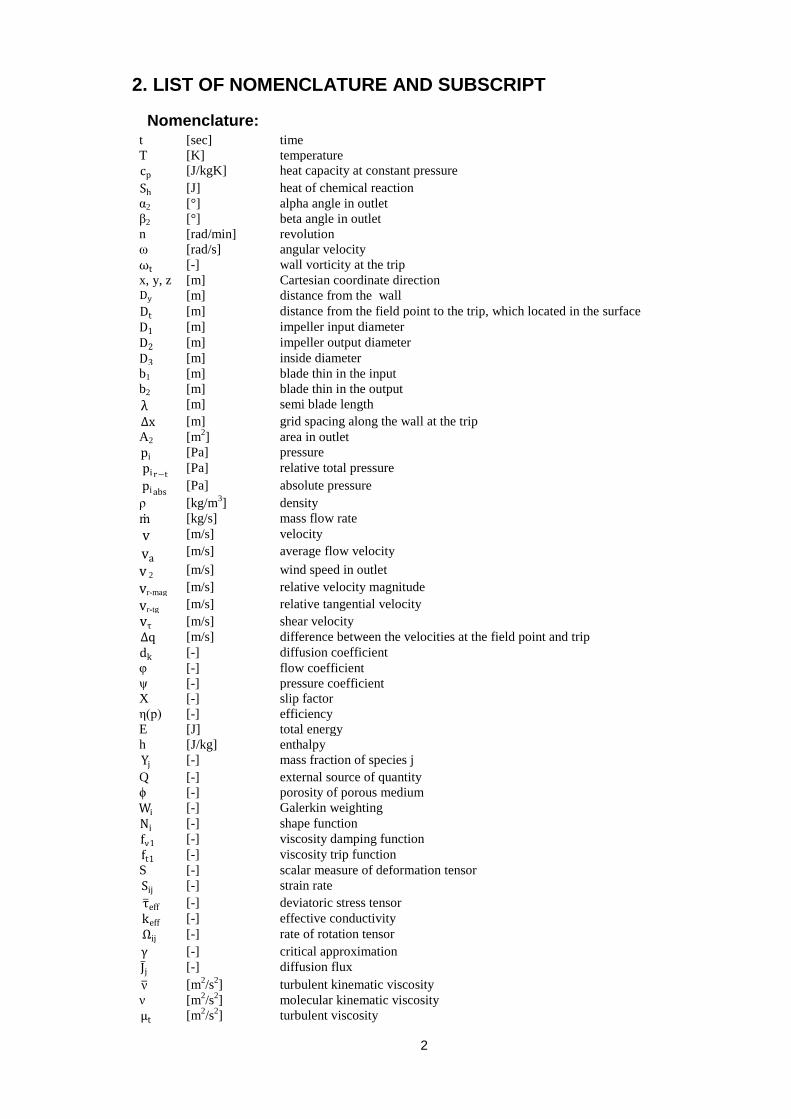
2. LIST OF NOMENCLATURE AND SUBSCRIPT
Nomenclature: t [sec] time
T [K] temperature
cp [J/kgK] heat capacity at constant pressure
Sh [J] heat of chemical reaction
α2 [°] alpha angle in outlet
β2 [°] beta angle in outlet
n [rad/min] revolution
ω [rad/s] angular velocity
ωt [-] wall vorticity at the trip
x, y, z [m] Cartesian coordinate direction Dy [m] distance from the wall
Dt [m] distance from the field point to the trip, which located in the surface
D1 [m] impeller input diameter
D2 [m] impeller output diameter
D3 [m] inside diameter
b1 [m] blade thin in the input
b2 [m] blade thin in the output
λ [m] semi blade length
∆x [m] grid spacing along the wall at the trip
A2 [m2] area in outlet
pi [Pa] pressure
pi r−t [Pa] relative total pressure
pi abs [Pa] absolute pressure
ρ [kg/m3] density
m [kg/s] mass flow rate
v [m/s] velocity
va [m/s] average flow velocity
v 2 [m/s] wind speed in outlet
vr-mag [m/s] relative velocity magnitude
vr-tg [m/s] relative tangential velocity
vτ [m/s] shear velocity
∆q [m/s] difference between the velocities at the field point and trip
dk [-] diffusion coefficient
φ [-] flow coefficient
ψ [-] pressure coefficient
X [-] slip factor
η(p) [-] efficiency
E [J] total energy
h [J/kg] enthalpy
Yj [-] mass fraction of species j
Q [-] external source of quantity
ϕ [-] porosity of porous medium
Wi [-] Galerkin weighting
Ni [-] shape function
fν1 [-] viscosity damping function
ft1 [-] viscosity trip function
S [-] scalar measure of deformation tensor
Sij [-] strain rate
τ eff [-] deviatoric stress tensor
keff [-] effective conductivity
Ωij [-] rate of rotation tensor
γ [-] critical approximation
J j [-] diffusion flux
ν [m2/s
2] turbulent kinematic viscosity
ν [m2/s
2] molecular kinematic viscosity
μt [m2/s
2] turbulent viscosity

3
Subscript: i, j, k [-] coordinate components
k [W/(m∙K)] conductivity
Gν [-] productivity of turbulent viscosity
Yν [-] distribution of turbulent viscosity

4
3. INTRODUCTION
The goal of final thesis to investigate a forward curved radial ventilator with
numerical methods. From the previous semester experience I learned the basics
about numeric simulation, and I would like to deepen my knowledge. My opinion is
with this store of learning man can get good job. In addition I would like to increase
my language knowledge too. Because of these two reasons I choose the
ERASMUS program.
In the thesis beside of experience I used several references. They are found in
the chapter of Bibliography. Most of allusion collected from user manuals and CFD
description, but the most useful was Aerodynamic performance of centrifugal fan
with forward curved blades. This work made by my consultant and supervisor.

5
4. DEFINITION AND CLASSIFICATION
4.1 General information about ventilators
The invention of ventilation was raised after the 2nd industrial revolution. In that
time the electric motor drive had appeared besides the conventional motor drive.
Traditionally the ventilators used in heavy industry especially in mining. The
classification did not followed the pace of development, and later it was troublous
for academics, engineers and administrators too. Until 1972 that Eurovent
produced its document 1/1 which gave agreed terms and definitions for fan sand
their components. This document was subsequently adopted by ISO and became
ISO 13348 [1].This standard proving can be sometimes limited, but for average
good this is fair enough. The biggest problem was to wrote the definition of what
exactly is a fan has proved difficult for the industry to accept [1]. But what is
exactly the difference between fan and compressor? According to Eurovent 1/1
and ISO 13348 is as follow:
“A fan is a rotary-bladed machine which receives mechanical energy and utilizes it
by means of one or more impellers fitted with blades to maintain a continuous flow
of air or other gas passing through it and whose work per unit mass does not
normally exceed 25 kJ/kg.”
Overall I should follow the experience of authors of “Fans & Ventilation a Practical
Guide”. His definition is:
“A fan is a rotary-bladed machine which delivers a continuous flow of air or gas at
some pressure, without materially changing its density.” [1]
After all the deviation is fairly thin between compressors and fans. ASME, in its
performance test Code PTC11 says that the boundary is “rather vague”.
AMCA/ASHRAE in Standard 210/51 state that “the scope has been broadened by
eliminating the upper limit of compression ratio”. Nevertheless, a boundary exists
somewhere. ISO/TC117 has proposed that a maximum absolute pressure rise of
30% should be adopted. This equates to 30 kPa when handling standard air. For
any others not yet fully metricated, this is about ~947000 mm water gauge.
However, there are machines which we would recognize as fans developing
pressures up to ~179068 mm water gauge or 60 kPa. Equally there are machines
recognizable as compressors developing less than 6 kPa. The prime function of a

6
fan is, therefore, to move relatively large volumes of air at pressures sufficient to
overcome the resistance of the systems to which they are attached. A fan’s
aerodynamic performance in terms of the pressure it generates as a functions of
flowrate, and how efficiently this is done, is what differentiates one fan type from
another. For any specific duty of flowrate and pressure rise, an infinite number of
fans of varying types could be offered. [1]
In general we have got the rules, how to design fans particularly impellers. The
units could be of small diameter running at high rotational speed or conversely
larger fans at low speeds. The selection of an appropriate fan will be influenced by
space availability, driving method, noise limitations, aerodynamic and mechanical
efficiency, mechanical strength and even, alas, capital cost and lead time [1]. In
manufacturing program the optimum setups cannot reach because of the
production‟s prize. In Figure 1 we can see the continuous range of aerodynamic
designs from low flowrate/ high pressure through to high flowrate/ low pressure.
Figure 1: End elevation of impellers showing variation with flowrate and pressure [1]
There is a continuing increase of inlet area available to the air from the narrow
centrifugal fans though to the propeller fans where the total swept area is open to
the flow [1]. The next I would like to show the main classification of ventilators. By
“Fans & Ventilation a Practical Guide” we can divide them though their impellers:
Propeller or axial flow where the effective movement of the air is straight
through the impeller at a constant distance from its axis. The major
component of blade force on the air is detected axially from the inlet to
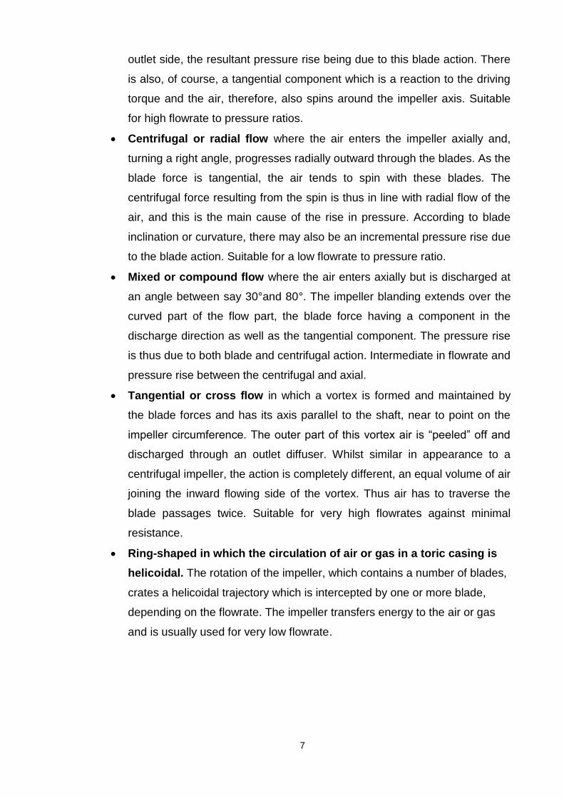
7
outlet side, the resultant pressure rise being due to this blade action. There
is also, of course, a tangential component which is a reaction to the driving
torque and the air, therefore, also spins around the impeller axis. Suitable
for high flowrate to pressure ratios.
Centrifugal or radial flow where the air enters the impeller axially and,
turning a right angle, progresses radially outward through the blades. As the
blade force is tangential, the air tends to spin with these blades. The
centrifugal force resulting from the spin is thus in line with radial flow of the
air, and this is the main cause of the rise in pressure. According to blade
inclination or curvature, there may also be an incremental pressure rise due
to the blade action. Suitable for a low flowrate to pressure ratio.
Mixed or compound flow where the air enters axially but is discharged at
an angle between say 30°and 80°. The impeller blanding extends over the
curved part of the flow part, the blade force having a component in the
discharge direction as well as the tangential component. The pressure rise
is thus due to both blade and centrifugal action. Intermediate in flowrate and
pressure rise between the centrifugal and axial.
Tangential or cross flow in which a vortex is formed and maintained by
the blade forces and has its axis parallel to the shaft, near to point on the
impeller circumference. The outer part of this vortex air is “peeled” off and
discharged through an outlet diffuser. Whilst similar in appearance to a
centrifugal impeller, the action is completely different, an equal volume of air
joining the inward flowing side of the vortex. Thus air has to traverse the
blade passages twice. Suitable for very high flowrates against minimal
resistance.
Ring-shaped in which the circulation of air or gas in a toric casing is
helicoidal. The rotation of the impeller, which contains a number of blades,
crates a helicoidal trajectory which is intercepted by one or more blade,
depending on the flowrate. The impeller transfers energy to the air or gas
and is usually used for very low flowrate.
8
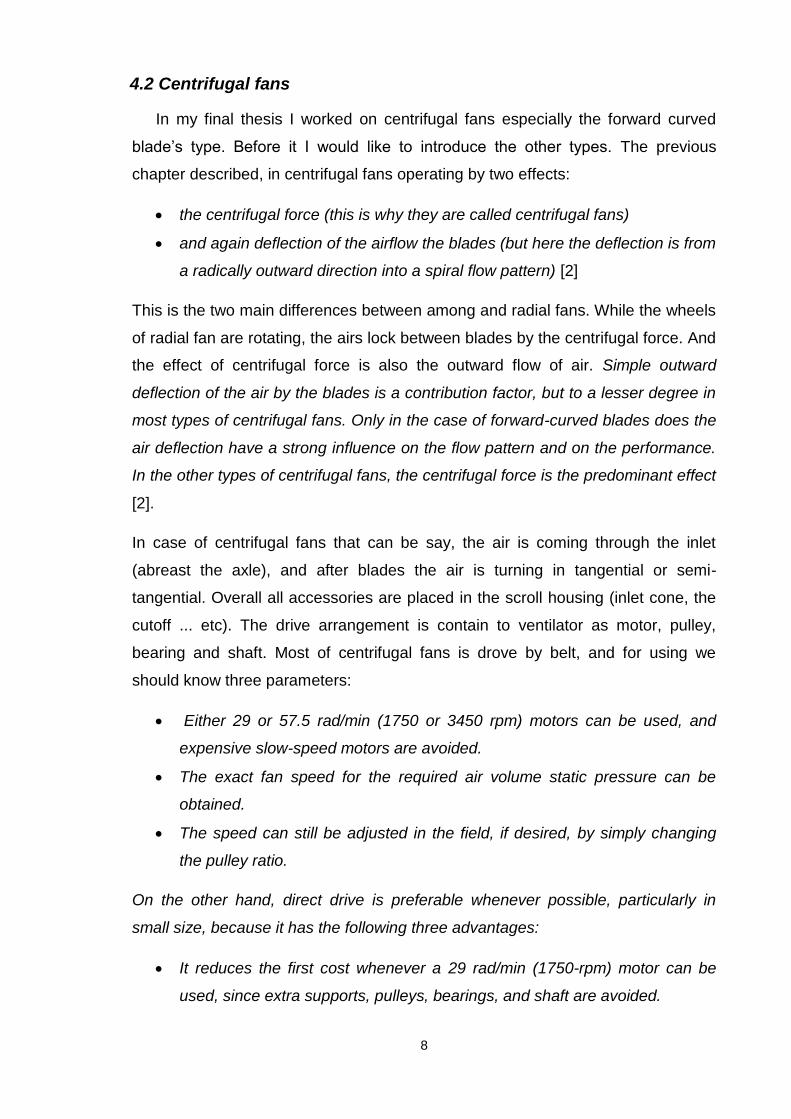
4.2 Centrifugal fans
In my final thesis I worked on centrifugal fans especially the forward curved
blade‟s type. Before it I would like to introduce the other types. The previous
chapter described, in centrifugal fans operating by two effects:
the centrifugal force (this is why they are called centrifugal fans)
and again deflection of the airflow the blades (but here the deflection is from
a radically outward direction into a spiral flow pattern) [2]
This is the two main differences between among and radial fans. While the wheels
of radial fan are rotating, the airs lock between blades by the centrifugal force. And
the effect of centrifugal force is also the outward flow of air. Simple outward
deflection of the air by the blades is a contribution factor, but to a lesser degree in
most types of centrifugal fans. Only in the case of forward-curved blades does the
air deflection have a strong influence on the flow pattern and on the performance.
In the other types of centrifugal fans, the centrifugal force is the predominant effect
[2].
In case of centrifugal fans that can be say, the air is coming through the inlet
(abreast the axle), and after blades the air is turning in tangential or semi-
tangential. Overall all accessories are placed in the scroll housing (inlet cone, the
cutoff ... etc). The drive arrangement is contain to ventilator as motor, pulley,
bearing and shaft. Most of centrifugal fans is drove by belt, and for using we
should know three parameters:
Either 29 or 57.5 rad/min (1750 or 3450 rpm) motors can be used, and
expensive slow-speed motors are avoided.
The exact fan speed for the required air volume static pressure can be
obtained.
The speed can still be adjusted in the field, if desired, by simply changing
the pulley ratio.
On the other hand, direct drive is preferable whenever possible, particularly in
small size, because it has the following three advantages:
It reduces the first cost whenever a 29 rad/min (1750-rpm) motor can be
used, since extra supports, pulleys, bearings, and shaft are avoided.

9
It avoids a 5 to 10 percent loss in brake horsepower, consumed by the belt
drive.
New belts usually stretch 10 to 15 percent in operation, requiring belt
adjustments. Direct drive avoids this maintenance [2].
In the following I would like to introduce the types of centrifugal fan‟s blade. By
Bleier we can separate six main types: airfoil (AF), backward-curved (BC),
backward inlet (BI), radial tip (RT), forward-curved (FC), and radial blade (RB). W
T W (Bill) Cory supplements to disunite the radial and backward curved blades. In
the next I will indicate the name of utility and the main type‟s short form.
In generally the designer have to decide which type is the best for using. Of course
the best choose is the low costs fan with the maximum efficiency. Best efficiency
can be reached by airfoil blades, and the worth is the radial type. For all duties the
higher initial cost of backward bladed fans can usually be recouped many times
over during the life of the unit, as the energy consumption will often be reduced by
25% compared with forward curved fans. Driving motors will also be smaller, and
as the fans have a non-overloading power characteristic only a small margin is
necessary over the absorbed power [1]
Figure 2: six blade shapes [1]
4.2.1 Airfoil or backward aerofoil blades (AF)
The impeller is shown in Figure 3. The blades produce lift forces, which
counteract inter-blade circulation without requiring precise angles. Thus smooth
flow conditions are maintained over a considerable portion of the characteristic [1].
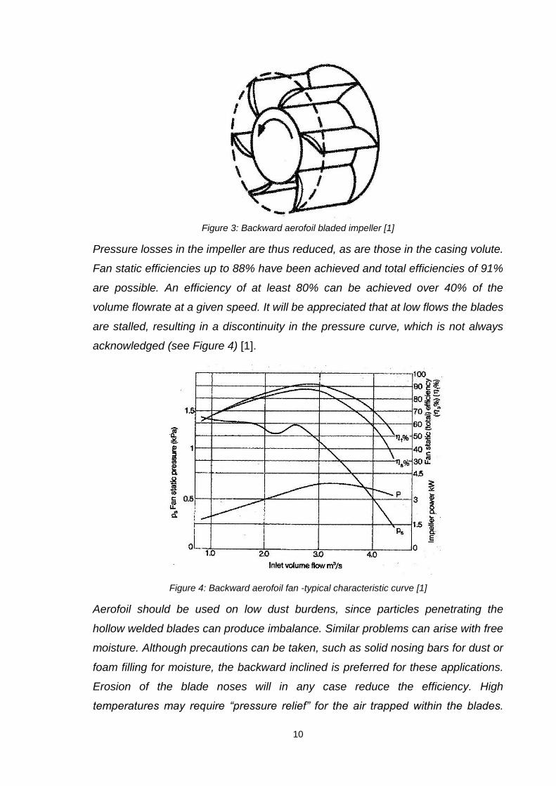
10
Figure 3: Backward aerofoil bladed impeller [1]
Pressure losses in the impeller are thus reduced, as are those in the casing volute.
Fan static efficiencies up to 88% have been achieved and total efficiencies of 91%
are possible. An efficiency of at least 80% can be achieved over 40% of the
volume flowrate at a given speed. It will be appreciated that at low flows the blades
are stalled, resulting in a discontinuity in the pressure curve, which is not always
acknowledged (see Figure 4) [1].
Figure 4: Backward aerofoil fan -typical characteristic curve [1]
Aerofoil should be used on low dust burdens, since particles penetrating the
hollow welded blades can produce imbalance. Similar problems can arise with free
moisture. Although precautions can be taken, such as solid nosing bars for dust or
foam filling for moisture, the backward inclined is preferred for these applications.
Erosion of the blade noses will in any case reduce the efficiency. High
temperatures may require “pressure relief” for the air trapped within the blades.

11
Whenever operating costs are of paramount importance, as when large powers
are involved and where is continuous operation at high load factor, the aerofoil is
to be preferred. In general the advantages are not significant for fans below size 1
m. Aerofoils may also be necessary when increased duty is required from existing
power lines: in many cases the power saved may allow a smaller motor to be
installed so that the overall cost is the same. In other cases the additional fan price
may be recovered in energy cost differences long before expiry of the period
allowed for amortizing plan costs [1].
4.2.2 Backward curved blades (BC)
These impellers are shown in Figure 5 and are preferred for certain
applications where there may be disadvantages in the use of the backward
inclined type. Due to the curvature, the blade angle at inlet can be made stepper
for a given outlet angle. This generally enables shock losses to be kept low, whilst
the curvature itself develops a certain degree of lift. It is therefore possible to
arrange such fans with a pressure curve continually rising to zero flow [1].
Figure 5: Backward curved bladed impeller [1]
They can be extremely stable, with none of the “bumps” in their curves found with
other types, and most suitable for operation in parallel on multi-fan plants. With the
special blade curvatures now used, efficiencies exceed 82% static, approaching
those attained by aerofoil bladed fans. The steeper inlet angle also results in a
stronger blade, which can rotate at higher speeds. This is offset to a large extent,
however, by the need to run at higher speeds for a given duty as compared with
the backward inclined type. They are also more expensive as, unless complex
press tools are used to “stretch” the metal, the blades cannot be flanged for
riveting or spot welding and have to be arc welded in position.

12
Figure 6: Backward curved fan -typical characteristics curves [1]
The curvature of backward curved blades (concave on the underside of the
blades) is inclined to encourage the build-up of dust. As the impeller in its rotation
tends to develop a positive pressure on the working convex face of the blade and
negative effect on the underside, dust can lodge within the camber. This becomes
more pronounced on the narrowest fans where the camber is substantial and the
chord is very much shorter than the developed blade length. The wider units have
less curvature, although the effects are offset by the shallow outlet angles.
Generally backward curved impellers are not so suitable for high temperature
operation, as differential expansion between blades and shrouds can be severe
inducing additional stresses. Gas temperatures should therefore be limited to 623
K. Other advantages are the same as those of the backward include type,
including a relatively steep pressure characteristic and non-overloading power
curve (see Figure 6) [1].
4.2.3 Reverse curve blades (BC)
These blades are backward curved at their tips but forward curved at the heel
(see Figure 7). Characteristics are generally similar to the backward curved type
with the same limitations to their use. Shock losses at entry to the blade passages
are reduced however and a slightly higher efficiency maintained outside the range
of the b.e.p [1].
13
Figure 7: Reverse curve bladed impeller [1]
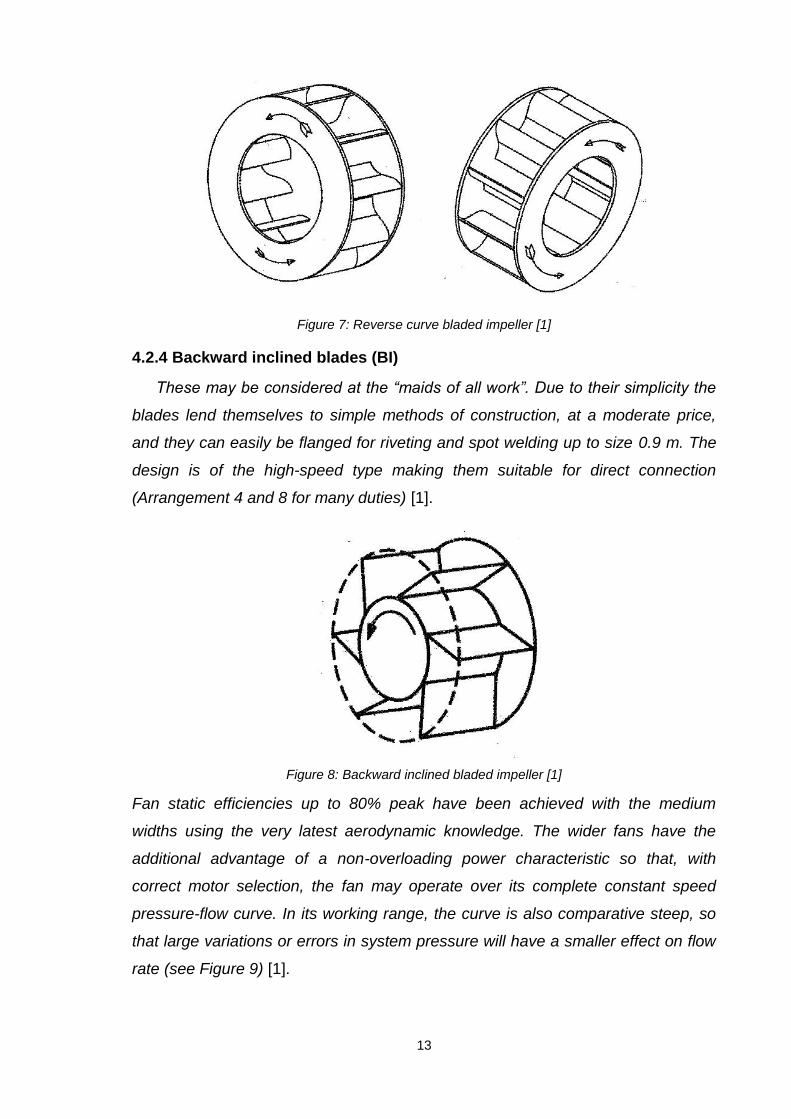
4.2.4 Backward inclined blades (BI)
These may be considered at the “maids of all work”. Due to their simplicity the
blades lend themselves to simple methods of construction, at a moderate price,
and they can easily be flanged for riveting and spot welding up to size 0.9 m. The
design is of the high-speed type making them suitable for direct connection
(Arrangement 4 and 8 for many duties) [1].
Figure 8: Backward inclined bladed impeller [1]
Fan static efficiencies up to 80% peak have been achieved with the medium
widths using the very latest aerodynamic knowledge. The wider fans have the
additional advantage of a non-overloading power characteristic so that, with
correct motor selection, the fan may operate over its complete constant speed
pressure-flow curve. In its working range, the curve is also comparative steep, so
that large variations or errors in system pressure will have a smaller effect on flow
rate (see Figure 9) [1].

14
Figure 9: Backward inclined bladed -typical characteristic curves [1]
The blades are self-cleaning to a certain degree and are in any case easy to clean
because of their single plate flat form. They are therefore suitable for free-flowing
granular dust burdens or moisture-laden air. In the absence of special factors, this
impeller is the recommended form for all applications including commercial and
industrial ventilation system, low and high velocity air conditioning, the clean side
of collectors in dust extract systems, fume extraction, etc.
Standard fans are available for operation at gas temperatures up to 623 K and
special units employing high temperature alloys can be custom-manufactured for
gases up to 773 K. In general terms, the narrower the impeller, the fewer the
number of blades and the greater the blade outlet angle. Both these factors are
conductive to the acceptance of higher dust burdens but counter-balanced to a
certain extent by boundary layer effects and higher abrasive velocities [1].
4.2.5 Radial tipped blades (RT)
This blade from is used as an alternative to the shrouded radial. Generally
there is an increasing number of blades and the heel of these is forward curved to
reduce shock losses. The efficiency and flowrate are therefore improved for a
given size, but the characteristics are otherwise similar. Fan static efficiencies up
to 73% are possible [1].
15
Figure 10: Radial tipped impellers [1]
The units are widely used for included draught on water tube boilers where low
efficiency dust collectors are incorporated. Dust burdens similar to those of the
shrouded radial [1].
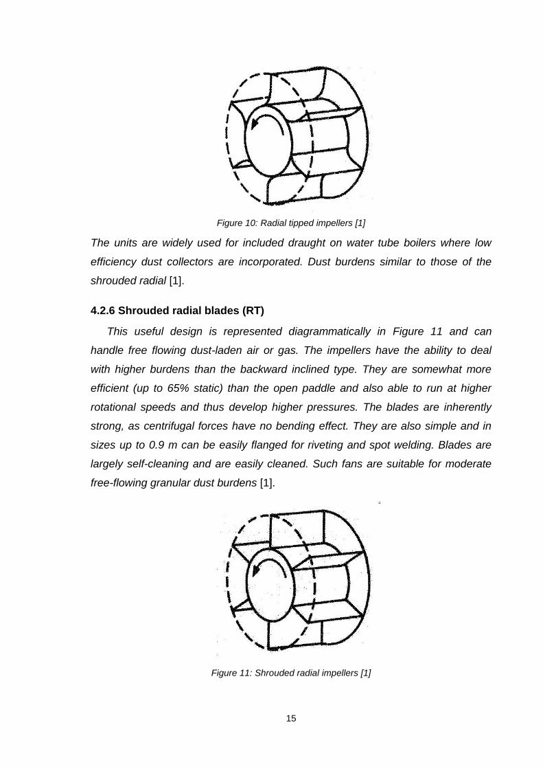
4.2.6 Shrouded radial blades (RT)
This useful design is represented diagrammatically in Figure 11 and can
handle free flowing dust-laden air or gas. The impellers have the ability to deal
with higher burdens than the backward inclined type. They are somewhat more
efficient (up to 65% static) than the open paddle and also able to run at higher
rotational speeds and thus develop higher pressures. The blades are inherently
strong, as centrifugal forces have no bending effect. They are also simple and in
sizes up to 0.9 m can be easily flanged for riveting and spot welding. Blades are
largely self-cleaning and are easily cleaned. Such fans are suitable for moderate
free-flowing granular dust burdens [1].
Figure 11: Shrouded radial impellers [1]

16
It should be noted that the power rises continually towards free air (zero pressure)
and a reasonable margin is necessary over the absorbed power, unless the
system pressure can be accurately assessed. As the impeller has a backplate,
wear is concentrated on this, but casing wear is correspondingly reduced
compared with the open paddle. Because of its characteristics, the shrouded radial
impeller is widely used in gas streams having a significant dust burden, for
example induced draught on rotary driers for the quarry and roadstone industries.
A typical characteristic curve is shown in Figure 12 [1].
Figure 12: Shrouded radial -typical characteristic curves [1]
4.2.7 Open paddle blades (RB)
This is the impeller for heavy dust burdens in excess of those possible with the
shrouded radial. Its efficiency is only moderate (up to 60% static) but it is suitable
for high temperatures. As there are no shrouds or backplates, the blades are free
to expand. Standard units may therefore be used with gases up to 623 K, but
special alloy wheels can be designed for the very highest temperatures [1].
17
Figure 13: Open paddle impellers [1]
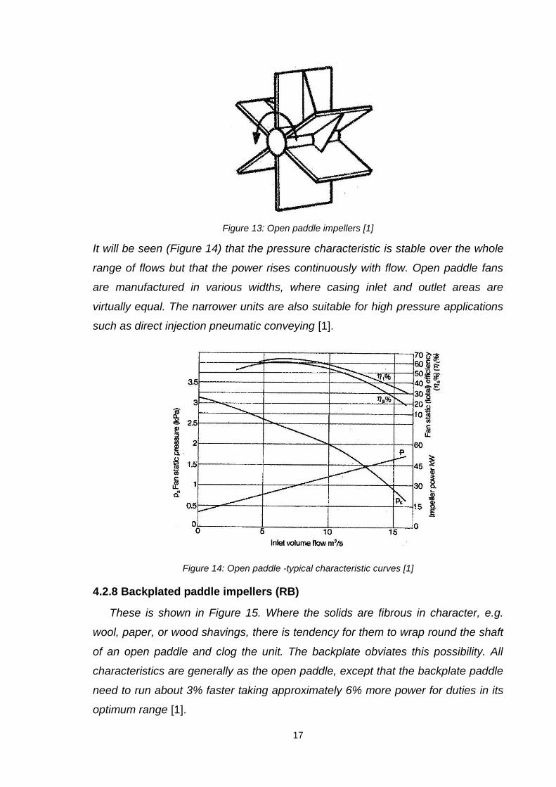
It will be seen (Figure 14) that the pressure characteristic is stable over the whole
range of flows but that the power rises continuously with flow. Open paddle fans
are manufactured in various widths, where casing inlet and outlet areas are
virtually equal. The narrower units are also suitable for high pressure applications
such as direct injection pneumatic conveying [1].
Figure 14: Open paddle -typical characteristic curves [1]
4.2.8 Backplated paddle impellers (RB)
These is shown in Figure 15. Where the solids are fibrous in character, e.g.
wool, paper, or wood shavings, there is tendency for them to wrap round the shaft
of an open paddle and clog the unit. The backplate obviates this possibility. All
characteristics are generally as the open paddle, except that the backplate paddle
need to run about 3% faster taking approximately 6% more power for duties in its
optimum range [1].

18
Figure 15: Backplated paddle impellers [1]
4.2.9 Forward curved (FC)
If we take BI blade and curve the outer portion in the forward direction of
rotation until the blade tip is radial, we will obtain a radial tip (RT) blade. If we now
continue curving the blade even more in the forward direction, we will obtain a
forward curved (FC) blade [2].
The main differs from the previous is in the ability of deliver. The forward curved
centrifugal fan has got much better skills (air volume, production static pressure)
than the other blade types (AF, BC, or BI) in the same size and speed. The
general fields of application are for heating (for furnace), for air conditioning
(ventilating), and for cooling of electric application or other equipment where the
low speed is needed to prevent the vibration.
They are used mainly in small and medium sizes 0.05- to 0.9 m wheel diameter (in
inch: 2 to 36 wheel diameter) where their lower efficiency is less objectionable but
occasionally in sizes up to 1.85 m wheel diameter (73-in). To accommodate the
airflow, which is large relative to size and speed, the diameter ratio D1/D2 is also
large, from 0,75 for small sizes to 0,90 for large size [2].
It means they have a large inside diameter D1 and a narrow annual space left for
blades. The narrow annulus calls for greater number of blades, usually between
0.6 (meter the small sizes) and 1.6 (meter the larger sizes). In other words, the
passages between adjacent blades are short and are made narrower (by using
more blades) for better guidance of the airflow. The shroud is a flat ring, so b1=b2.
The shroud inside diameter is often slightly larger than the blade inside diameter
so that portions of the blades protrude inward beyond the shroud inside diameter.

19
This will somewhat improve the flow conditions by leaving more room for the right-
angle turn from axial to radially outward. The inlet clearance is made larger than
for AF, BC, BI or RT fans. The maximum blade width is large, often as much as 65
percent of the blade inside diameter D1 [2].
The blade angles are very large to obtain the large air volume. At the leading
edge, the blade angle β1 is usually between 80° and 120°, so the relative airflow
hits the leading edge of the blade at a large, unfavorite angle, far from any
tangential condition, At the blade tip, the blade angle β2 is even larger, between
120°and 160°. This results in a large and almost circumferential (about 20° from
circumferential) absolute air velocity v2 at the blade tip. v2 is larger than the tip
speed, i.e., the velocity of the blade tip itself. This is a result of the scooping action
of the blades. The scroll housing is the same size and shape as for AF, BC, and BI
fans, but the cutoff protrudes higher into the outlet. The large air velocity v2 (kinetic
energy) is gradually slowed down in the scroll housing and partially converted into
static pressure (potential energy). A good portion of the static pressure is
produced in the scroll housing as a result of this conversion from velocity pressure
into static pressure. For this reason, FC centrifugal fans can function properly only
in a scroll housing. For radial discharge, as in plug fans or in roof ventilators, AF,
BC, and BI centrifugal fans can be used, but not FC fans (see Figure 16) [2].
Figure 16: Performance curves for typical FC centrifugal fan [2]
The main reason for the lower efficiency of FC fans is that the airflow through the
blade channels of FC fans has to change its direction by almost 180°, i.e. more

20
than in other centrifugal fan types. The air stream can hardly follow the strong
curvature of the blades, tangential conditions are no longer prevailing, and the flow
is far from being smooth. It is more turbulent than in AF, BC, BI, or RT fans.
Because the fan efficiency is comparatively low anyway, slight manufacturing
inaccuracies will not reduce is much further and therefore will be less
objectionable than with BI blades. Aerodynamic conditions are often secondary in
the design of FC fans. Refinements such as overlapping at the inlet, slopping of
the shroud, and so on can be left out [2].
The shape of FC blades is a smooth curve: In small sizes, it is a simple circular
arc; in larger sizes, a shape with more curvature near the leading edge is of
advantage, since it results in a gradual expansion of the blade channel at a more
even rate [2]. Figure 17 shows a comparison of four static pressure curves, all for
0.69 meter wheel diameters. You will note the following:
1. At 19 rad/min (1140 rpm), the RT fan delivers slightly more air volume
and produces slightly more static pressure than the BI fan, but the FC fan
delivers considerably more air volume (about 2,5 times as much) and
produces a much higher maximum static pressure (about double) than
the BI fan. This, as mentioned previously, is at the expense of a lower
efficiency for the FC fan.
2. If the FC fan runs at half the speed, the static pressure curve covers a
range comparable with that of the BI fan. To be more specific, the FC fan
at 9.5 rad/min (570 rpm) still delivers about 28 percent more air volume
at free delivery, and the maximum static pressure is about one-half. It
should be mentioned that the FC fan has a much higher noise level than
a BI fan of the same size and speed due to the highly turbulent airflow.
The noise level than BI fan of the same size and speed due to the highly
turbulent airflow. The noise levels of the two fans are only comparable if
the FC fan runs at half the speed.
3. The static pressure curve of the FC fan has a dip that in some
installations may cause unstable operation. Precaution, therefore, should
be taken so that FC fans are not used for applications such as fluctuating
systems or parallel operation and that even in other installations the will
not operate in the unstable range of the static pressure curve.

21
Figure 17: Comparison of static pressure curves for BI, RT, and FC centrifugal fans, 27-in wheel diameter [2]
Figure 16 shows the complete performance (static pressure, brake horsepower,
efficiency, and sound level versus air volume) for a 0.69 m FC fan at 9.5 rad/min.
Note that the air volume scale here is double that in Figure 17. You will note the
following [2]:
1. The brake horsepower curve is overloading in the low-pressure range. At
free delivery, the brake horse power is more than twice the brake
horsepower in the range of maximum efficiency. This shape of the brake
horsepower curve results in power requirements outside the operating
range that are higher by fan than those within the operating range. While
centrifugal fans in general are not built for operation at or near free
delivery (propeller fans or turbeaxial fans perform this function with
greater efficiency and at lower cost), the overloading brake horsepower
curve is a serious disadvantage of FC fans. In small sizes, an oversize
motor with a horsepower rating equal to the maximum brake horsepower
at free delivery is normally selected so that operation at any condition will
be safe. For larger units, however, the increased price of the oversized
motor would be prohibitive, and the motor horsepower is selected only
slightly larger than the brake horsepower for the prospective operating
condition. Precaution must be taken so that the unit, when installed in the
field, will not operate against too low a static pressure because this would
result in an overload for the motor. The permissible operating range of
the FC fan, being limited to the left by the dip in the static pressure curve

22
and to the right by the rising brake horsepower curve, therefore, is
narrower than that of AF, BC, or BI fans.
2. The sound-level curve has its minimum in the range of best efficiencies.
3. Note the dashed line, indicating a poor performance, if an FC fan were
used for circumferential discharge, i.e., without a scroll housing, as in
plug fans or roof ventilators. Without a scroll housing, AF, BC, and BI
fans will deliver larger air volumes, but FC fans would deliver smaller air
volumes because they need the scroll housing to convert some of the
high air velocity at the blade tips into additional static pressure. Without
this conversion, the FC fan will have a poor performance, as shown by
dashes in Figure. 16.
If we would like to summarize by Frank P Bleier P.E, we can say that BC and BI
blades have the following advantages over FC blade:
1. Stable static pressure curve (no dip)
2. Higher efficiencies, resulting in lower operating costs
3. Non-overloading brake horsepower characteristic
4. Higher operating speeds, which for direct drive may result in less
expensive motors [2]
On the other hand FC blades have to following benefits over BC and BI blades:
1. Compactness
2. Lower running speeds, resulting in easier balancing
3. Lower first cost, particularly in small sizes [2]
From the preceding it appears that either type (BI or FC) has its advantages for
certain applications. In small sizes, the advantages of FC fans will outweigh their
disadvantages. In larger sizes, however, the BI fan will be preferable. The RT fan
takes the place between BI and FC fans, but – as indicated in Figure 17 – it is
closer to the BI fan. This intermediate condition is true for performance, brake
horsepower, efficiency, and sound level, The RT fan, however, is a more rugged
unit than either the BI or the FC fan and therefore can tolerate higher running
speeds (resulting in high static pressures), higher temperatures, and serve service
conditions. RT fans are often employed for conveying materials, such as gridding
dust, saw dust, cotton, grains, and shavings, if the blades are spaced far enough
23
from each other so that narrow passages are avoided, which would tend to
become plugged up by deposits of dirt or of the material conveyed [2].
4.3.0 Deep vane forward curved (FC)
Figure 18: Deep vane forward curved impellers [1]
These blades are considerably stronger than the conventional forward cured,
being triangulated. They can thus run at higher speeds developing high pressure.
A more detailed impeller drawing is shown in Figure 17, which perhaps explains
why there is some reduction in flowrate. Nevertheless a more stable
pressure/flowrate curve is produced albeit with a moderate peak efficiency [1].
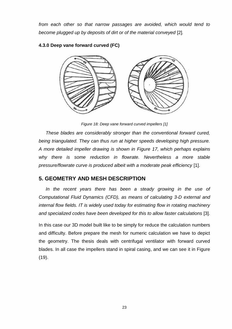
5. GEOMETRY AND MESH DESCRIPTION
In the recent years there has been a steady growing in the use of
Computational Fluid Dynamics (CFD), as means of calculating 3-D external and
internal flow fields. IT is widely used today for estimating flow in rotating machinery
and specialized codes have been developed for this to allow faster calculations [3].
In this case our 3D model built like to be simply for reduce the calculation numbers
and difficulty. Before prepare the mesh for numeric calculation we have to depict
the geometry. The thesis deals with centrifugal ventilator with forward curved
blades. In all case the impellers stand in spiral casing, and we can see it in Figure
(19).
24
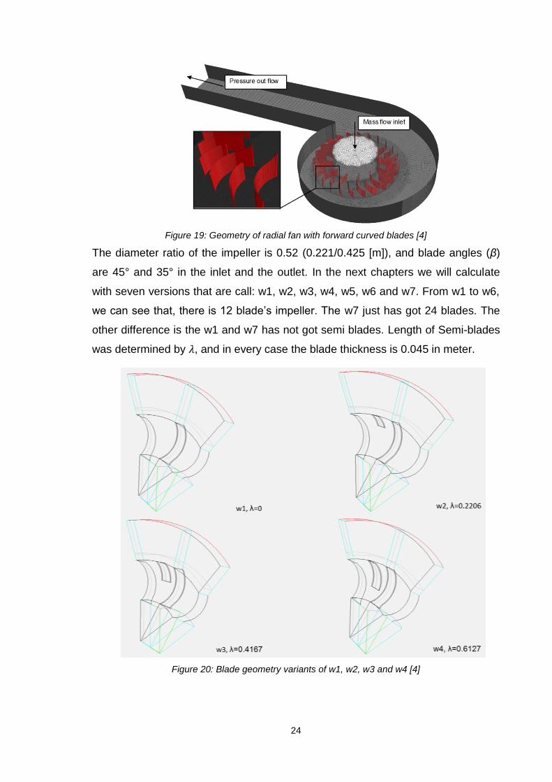
Figure 19: Geometry of radial fan with forward curved blades [4]
The diameter ratio of the impeller is 0.52 (0.221/0.425 [m]), and blade angles (β)
are 45° and 35° in the inlet and the outlet. In the next chapters we will calculate
with seven versions that are call: w1, w2, w3, w4, w5, w6 and w7. From w1 to w6,
we can see that, there is 12 blade‟s impeller. The w7 just has got 24 blades. The
other difference is the w1 and w7 has not got semi blades. Length of Semi-blades
was determined by 𝜆, and in every case the blade thickness is 0.045 in meter.
Figure 20: Blade geometry variants of w1, w2, w3 and w4 [4]

25
Figure 21: Blade geometry variants of w5, w6 and w7 [4]
The semi-blades length calculated by this expression:
𝜆 = 𝐷2 − 𝐷3 𝐷2 − 𝐷1 (5.1)
From the above expression value of 𝜆 was changed between 22% and 92% of the
𝐷2. We can see that in the Figures (23, 13, 43, 44), and in the Figure (45) there
are diameter values.
Figure 22: Geometry of blades and semi-blades [4]
We can see more information in Figures 23 and 24.These was copied from
ANSYS FLUENT 13 with Mesh/Check, Mesh/Info/Quality, Mesh/Info/Size and the
Mesh/Info/Memory Usage commands.

26
Figure 23: Information about mesh size and quality
Figure 24: Memory usage of mesh
27
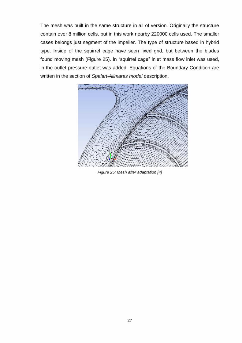
The mesh was built in the same structure in all of version. Originally the structure
contain over 8 million cells, but in this work nearby 220000 cells used. The smaller
cases belongs just segment of the impeller. The type of structure based in hybrid
type. Inside of the squirrel cage have seen fixed grid, but between the blades
found moving mesh (Figure 25). In “squirrel cage” inlet mass flow inlet was used,
in the outlet pressure outlet was added. Equations of the Boundary Condition are
written in the section of Spalart-Allmaras model description.
Figure 25: Mesh after adaptation [4]

28
6. THEORETICAL BACKGROUND OF NUMERICAL INVESTIGATION
This Section help to understand the basic equations. For solving the numerical
calculation we set for type pressure based coupled solver, and time steady state. If
we are using pressure based solver, we have to know: The solution process for
the pressure-based coupled solver (Figure 26) begins with a two-step initialization
sequence that is executed outside the solution iteration loop. This sequence
begins by initializing equations to user-entered (or default) values taken from the
ANSYS FLUENT user interface. Next, PROFILE UDFs are called, followed by a
call to INIT UDFs. Initialization UDFs overwrite initialization values that were
previously set [5].
Figure 26: Solution Procedure for the Pressure-Based Coupled Solver [5]

29
6.1 Steady-State description
6.1.1 General remarks
First of all we had to be classified the various types of flow. The classification
depends upon the variability or constancy of the velocity with time. We had to got
two case for describe the flow. In steady-flow (-state) the property values at
location in the flow are constant and the values do not vary with time. The
pressure or velocity at a point remains constant with time.
These can be denote as p = p(x, y, z), v = v(x, y, z) … etc. In steady flow the
appearance of the flow field recorded at different times will be identical. In the case
of unsteady flow, the properties vary with time p = p(x, y, z, t), v = v(x, y, z, t)
where t is time. In unsteady flow the picture of the flow field will vary with time and
will be constantly changing. In turbulent flow the pressure (or velocity) at any point
fluctuates around a mean value, but the mean value at a point over a period of
time is constant. For practical purposes turbulent flow is considered as steady flow
as long as the mean value of properties do not vary with time.
In our calculation we used steady-state‟s equation, whereas unsteady computation
needed. For both state we have to know the scalar equation of the form which is
the basic model of the present chapter:
𝜕𝜙
𝜕𝑡+
𝜕 𝑣𝑖𝜙
𝜕𝑥𝑖−
𝜕
𝜕𝑥 𝑖 𝑑𝑘
𝜕𝜙
𝜕𝑥 𝑖 + 𝑄
≡𝜕𝑣
𝜕𝑡+
𝜕 𝑣𝑥𝜙
𝜕𝑥+
𝜕 𝑣𝑦𝜙
𝜕𝑦−
𝜕
𝜕𝑥 𝑑𝑘
𝜕𝜙
𝜕𝑥 −
𝜕
𝜕𝑦 𝑑𝑘
𝜕𝜙
𝜕𝑦 + 𝑄 = 0 (6.1)
In this equation 𝑣𝑖 in general is a known velocity filed, 𝜙 is a quantity being
transported by this velocity in a convective manner or by diffusion action, where 𝑑𝑘
is the diffusion coefficient. In the above term Q represents any external sources of
the quantity 𝜙 being admitted to the system and also the reaction loss or gain
which itself is dependent on the concentration 𝜙.
The equation can be rewritten in a slightly modified form in which the convective
term has been differentiated as
𝜕𝜙
𝜕𝑡+ 𝑣𝑖
𝜕𝜙
𝜕𝑥𝑖+ 𝜙
𝜕𝑣𝑖
𝜕𝑥𝑖−
𝜕
𝜕𝑥 𝑖 𝑑𝑘
𝜕𝜙
𝜕𝑥 𝑖 + 𝑄 = 0 (6.2)

30
We will note that in the above form the problem is self-adjoint with the exception of
a convective term which is painted to red. The third term disappears if the flow
itself is such that its divergence is zero, i.e. if
𝜕𝑣𝑖
𝜕𝑥𝑖= 0 (summation over i implied) (6.3)
In what follows we shall discuss the scalar equation in much more detail as many
of the finite element remedies are only applicable to such scalar problems and are
not transferable to the vector forms [6]. From Equations (5.2) and (5.3) we have
𝜕𝜙
𝜕𝑡+ 𝑣𝑖
𝜕𝜙
𝜕𝑥𝑖−
𝜕
𝜕𝑥 𝑖 𝑑𝑘
𝜕𝜙
𝜕𝑥 𝑖 + 𝑄 = 0 (6.4)
The equation now considered is the steady-state version if Equation 6.1 i.e:
𝑣𝑥𝜕𝜙
𝜕𝑥+ 𝑣𝑦
𝜕𝜙
𝜕𝑦−
𝜕
𝜕𝑥 𝑑𝑘
𝜕𝜙
𝜕𝑥 −
𝜕
𝜕𝑦 𝑑𝑘
𝜕𝜙
𝜕𝑦 + 𝑄 = 0 (6.5a)
it two dimensions or more generally using indicial notation
𝑣𝑖𝜕𝜙
𝜕𝑥 𝑖−
𝜕
𝜕𝑥 𝑖 𝑑𝑘
𝜕𝜙
𝜕𝑥 𝑖 + 𝑄 = 0 (6.5b)
in both two and three dimensions. For apply further the above equations we used
Streamline Petrov-Galerkin method; because 𝑑𝑘 > 0, which is equivalent to
imposing a zero conduction flux at the outlet edge.
6.1.2 Streamline (Upwind) Petrov-Galerkin weighting (SUPG) The basic revelation about SUPG [6]: the Galerkin weighting (𝑊𝑖) is not equal
with shape function (𝑁𝑖), that is 𝑊𝑖 ≠ 𝑁𝑖 . Therefore we have to use this term
𝑊𝑖 = 𝑁𝑖 + 𝛾𝑊𝑖∗ (6.6)
where 𝑊𝑖∗ is the various form.
Wi∗
Ωedx = ±
h
2 (6.7)
The Equations (5.6) and (5.7) are possible to apply, but the most convenient is the
following simple definition which is, of course, a discontinuous function
𝛾𝑊𝑖∗ = 𝛾
2
𝑑𝑁𝑖
𝑑𝑥 sign 𝑣 (6.8)

31
Of course these rules are available in two and three dimension too. In three
dimension the convection is only active in the direction of the resultant element
velocity 𝑣, and hence the corrective, or balancing, diffusion introduced of the
upwinding should be anisotropic with a coefficient different from zero only in the
direction of the velocity resultant. This innovation introduced simultaneously by
Hughes and Brooks and Kelly can be readily accomplished by taking the individual
weighting function as [6]
𝑊𝑘 = 𝑁𝑘 + 𝛾𝑊𝐾∗ = 𝑁𝑘 +
𝛾
2
𝑣1 𝜕𝑁𝑘𝜕𝑥1
+𝑣2 𝜕𝑁𝑘𝜕𝑥2
𝑣 ≡ 𝑁𝑘 +
𝛾
2
𝑣𝑖
𝑣
𝜕𝑁𝑘
𝜕𝑥𝑖 (6.10)
where 𝛾 is determined for each element by the previously found expression written
as follows:
𝛾 = 𝛾𝑜𝑝𝑡 = coth 𝑃𝑒 −1
𝑃𝑒 (6.11)
with
𝑃𝑒 = 𝑣
2𝑘 (6.12)
and
𝑣 = 𝑣12 + 𝑣2
2 1 2 or 𝑣𝑖𝑣𝑖 (6.13)
The above expressions presuppose that the velocity components 𝑣1 and 𝑣2 in a
particular element are substantially constant and that the element size h can be
reasonably defined. The form of Equation (5.10) is such that the “non-standard”
weighting W* has a zero effect in the direction in which the velocity component is
zero. Thus the balancing diffusion is only introduced in the direction of the
resultant velocity (convective) vector 𝑣 . This can be verified if Fig. (15) is written in
tensional (indicial) notation as [6]:
𝑣𝑖𝜕𝜙
𝜕𝑥 𝑖−
𝜕
𝜕𝑥 𝑖 𝑑𝑘
𝜕𝜙
𝜕𝑥 𝑖 + 𝑄 = 0 (6.14)
In the discretized form the “balancing diffusion” term (obtained from weighting the
first term of the above with W of Equation 6.10) becomes
∂N
∂xiΩk ij
∂N
∂x jdΩ (6.15)

32
with
𝑘 𝑖𝑗 =𝛼𝑈𝑖𝑈𝑗
𝑈
2 (6.16)
This indicates a highly anisotropic diffusion with zero coefficients normal to the
convective velocity vector directions. It is therefore named the streamline
balancing diffusion or streamline upwind Petrov-Galerkin process.
The streamline diffusion should allow discontinuities in the direction normal to the
streamline to travel without appreciable distortion. However, with the standard
finite element approximations actual discontinuities cannot be modeled and in
practice some oscillations may develop when the function exhibits “shock like”
behavior. For this reason it is necessary to add some smoothing diffusion in the
direction normal to the streamlines and some investigation make appropriate
suggestions. The material validity of the procedures introduced in this section has
been established by Johnson et.al. for 𝛾 = 1, showing convergence improvement
over the standard Galerkin process. However, the proof does not include any
optimality in the selection of α values as shown by Equation 6.11 [6].
6.2 Spalart-Allmaras model
For describing the model I used two main sources: the Computational Fluid
Dynamics Volume III Fourth Edition book for describe the model [14], and
FLUENT 13‟s Documentation Descriptions [7], [8], [9], [10], [13], [15], [16], [17].
6.2.1 Overview
The Spalart-Allmaras model is a one-equation model that solves a modeled
transport equation for the kinematic eddy (turbulent) viscosity. The Spalart-
Allmaras model was designed specifically for aerospace applications involving
wall-bounded flows and has been shown to give good results for boundary layers
subjected to adverse pressure gradients. It is also gaining popularity in
turbomachinery applications. The Spalart-Allmaras model was developed for
aerodynamic flows. It is not calibrated for general industrial flows, and does
produce relatively larger errors for some free shear flows, especially plane and
round jet flows. In addition, it cannot be relied on to predict the decay of
homogeneous, isotropic turbulence [7].

33
6.2.2 Transport Equation for the Spalart-Allmaras Model The transported variable in the Spalart-Allmaras model, 𝜈 , is identical to the
turbulent kinematic viscosity except in the near-wall (viscosity-affected) region.
The transport equation for 𝜈 is
𝜕
𝜕𝑡 𝜌𝜈 +
𝜕
𝜕𝑥𝑖 𝜌𝜈 𝑣𝑖 = 𝐺𝜈 +
1
𝜍𝜈
𝜕
𝜕𝑥𝑗 𝜇 + 𝜌𝜈
𝜕𝜈
𝜕𝑥𝑗 + 𝐶𝑏2
𝜕𝜈
𝜕𝑥𝑗
2
− 𝑌𝜈 + 𝑆𝜈 (6.17)
where 𝐺𝜈 is the production of turbulent viscosity, and 𝑌𝜈 is the destruction of
turbulent viscosity that occurs in the near-wall region due to wall blocking and
viscous damping 𝜍𝜈 and 𝐶𝑏2are the constants and ν is the molecular kinematic
viscosity 𝑆𝜈 is a user-defined source term [8].
6.2.3 Modeling the Turbulent Viscosity This section used the [9] source. The turbulent viscosity, 𝜇𝑡 , is computed from
𝜇𝑡 = 𝜌𝜈 𝑓𝑣1 (6.18)
where the viscosity damping function, 𝑓𝑣1, is given by
𝑓𝑣1 =𝐵3
𝐵3+𝑐𝑣13 (6.19)
and
𝐵 ≡𝜈
𝜈 (6.20)
6.2.4 Modeling the Turbulent Production The production term, 𝐺𝜈 , is modeled as
𝐺𝜈 = 𝐶𝑏1𝜌𝑆 𝜈 (6.21)
where
𝑆 ≡ 𝑆 +𝜈
𝜅2𝐷2𝑓𝑣2 (6.22)
and
𝑓𝑣2 = 1 −𝑥
1+𝑥 𝑓𝑣1 (6.23)

34
𝐶𝑏1 and κ are constants, 𝐷𝑦 is the distance from the wall, and S is a scalar
measure of the deformation tensor. By default in ANSYS FLUENT, as in the
original model proposed by Spalart and Allmaras, S is based on the magnitude of
the vorticity:
𝑆 ≡ 2𝛺𝑖𝑗𝛺𝑖𝑗 (6.24)
where 𝛺𝑖𝑗 is the mean rate of rotation tensor and is defined by
𝛺𝑖𝑗 = 1
2 𝜕𝑢𝑖
𝜕𝑥𝑗−
𝜕𝑢𝑗
𝜕𝑥𝑖 (6.25)
The justification for the default expression for S is that, for shear flows, vorticity
and strain rate are identical. Vorticity has the advantage of being zero in inviscid
flow regions like stagnation lines, where turbulence production due to strain rate
can be unphysical. However, an alternative formulation has been proposed [10]
and incorporated into ANSYS FLUENT. This modification combines the measures
of both vorticity and the strain tensors in the definition of S [10]:
𝑆 ≡ 𝛺𝑖𝑗 + 𝐶𝑝𝑟𝑜𝑑 min 0, 𝑆𝑖𝑗 − 𝛺𝑖𝑗 (6.26)
where
𝐶𝑝𝑟𝑜𝑑 = 2.0, 𝛺𝑖𝑗 ≡ 2𝛺𝑖𝑗 𝛺𝑖𝑗 , 𝑆𝑖𝑗 ≡ 2𝑆𝑖𝑗𝑆𝑖𝑗 (6.27)
with the mean strain rate, 𝑆𝑖𝑗 , defined as
𝑆𝑖𝑗 = 1
2 𝜕𝑢𝑖
𝜕𝑥𝑗−
𝜕𝑢𝑗
𝜕𝑥𝑖 (6.28)
Including both the rotation and strain tensors reduces the production of eddy
viscosity and consequently reduces the eddy viscosity itself in regions where the
measure of vorticity exceeds that of strain rate [10].
6.2.5 Modeling the Turbulent Destruction
The equations was written from [12] source. The destruction model as
𝑌𝜈 = 𝐶𝑤1𝜌𝑓𝑤 𝜈
𝑑
2
(6.29)
where

35
𝑓𝑤 = 𝑔 1+𝐶𝑤3
6
𝑔6+𝐶𝑤36
1 6
(6.30)
𝑔 = 𝑟 + 𝐶𝑤2 𝑟6 − 𝑟 (6.31)
𝑟 =ν
𝑆 𝜅2𝑑2 (6.32)
𝐶𝑤1, 𝐶𝑤2 , and 𝐶𝑤3 ,are constants, and 𝑆 is given by Equation 6.21. Note that the
modification described above to include the effects of mean strain on S will also
affect the value of 𝑆 used to compute r. If the r a large value (about 10), we have
to expand Equation (5.32). For this case I suggest to use Computational Fluid
Dynamics Volume III Fourth Edition book [13]. For better use we have to vary the
Equation (134)
𝜕𝜈
𝜕𝑡=
1
𝜍𝜈 𝛻 ∙ 𝜈 + 𝜈 𝛻𝜈 + 𝐶𝑏2 𝛻𝜈 2 +𝐶𝑏1𝑆 𝜈 1 − 𝑓𝑡2
− 𝐶𝑤1𝑓𝑤 − 𝐶𝑏1𝑓𝑡2 𝜅2 𝜈 𝐷 2 + 𝑓𝑡1 𝛥𝑞 2 (6.33)
Where the function 𝑓𝑡2 is given by
𝑓𝑡2 = 𝑐𝑡3𝑒𝑥𝑝 −𝑐𝑡4𝐵2 (6.34)
𝑓𝑡1 = 𝑐𝑡1𝑔1𝑒𝑥𝑝 −𝑐𝑡2 𝜔𝑡
𝛥𝑞
2 𝐷2 + 𝑔𝑡
2𝐷𝑡2 (6.35)
The following are used in Equation (6.35):
𝐷𝑡 : The distance from the field point to the trip, which is located in the surface.
𝜔𝑡 : The wall vorticity at the trip.
𝛥𝑞: The difference between the velocities at the field point and trip
𝑔𝑡 : 𝑔𝑡 = min 1.0, 𝛥𝑞/𝜔𝑡𝛥𝑥 , where 𝛥𝑥 is the grid spacing along the wall at the
trip.
6.2.5 Model Constants
The constants used in the equations above are
𝐶𝜈1 = 7.1, (6.36)
𝜍𝜈 =2
3, 𝜅 = 0.41 (6.37)
𝐶𝑏1 = 0.1355, 𝐶𝑏2 = 0.622 (6.38)
𝐶𝑤1 =𝐶𝑏1
𝜅2 + (1 + 𝐶𝑏2)/𝜍𝜈 , 𝐶𝑤2 = 0.3, 𝐶𝑤3 = 2 (6.39)

36
𝐶𝑡1 = 1.0, 𝐶𝑡2 = 2.0, 𝐶𝑡3 = 1.1, 𝐶𝑡4 = 2.0 (6.40)
This forms copied from [13] source.
6.2.6 Wall Boundary Conditions
At walls, the modified turbulent kinematic viscosity, 𝜈 , is set to zero. When the
mesh is fine enough to resolve the viscosity-dominated sublayer, the wall shear
stress is obtained from the laminar stress-strain relationship [14]:
𝑣
𝑣𝑡=
𝜌𝑣𝜏𝐷𝑦
𝜇 (6.41)
If the mesh is too coarse to resolve the viscous sublayer, then it is assumed that
the centroid of the wall-adjacent cell falls within the logarithmic region of the
boundary layer, and the law-of-the-wall is employed [14]:
𝑣
𝑣=
1
𝜅ln𝐸𝑘
𝜌𝑣𝜏𝐷𝑦
𝜇 (6.42)
where v is the velocity parallel to the wall, 𝑣𝜏 is the shear velocity, 𝐷𝑦 is the
distance from the wall, κ is the von Kármán constant (0.4187), and 𝐸𝑘 = 9.793.
6.3 Energy equation
In ANSYS FLUENT for describe the convective heat and mass transfer we use
the energy equation. The basic form of the energy equation is:
𝜕
𝜕𝑡 𝜌𝐸 + 𝑉 ∙ 𝜈 𝜌𝐸 + 𝑝
= 𝑉 ∙ 𝑘𝑒𝑓𝑓 𝑉 𝑇 − 𝑗𝑗 𝐽𝑗 + 𝜏 𝑒𝑓𝑓 𝜈 + 𝑆 (6.43)
This is good start for special case. The turbulent heat transport is modeled using
the concept of the Reynolds’ analogy to turbulent momentum transfer. The
“modeled” energy equation is as follows [15]
𝜕
𝜕𝑡 𝜌𝐸 +
𝜕
𝜕𝑥𝑖 𝑣𝑖 𝜌𝐸 + 𝑝 =
𝜕
𝜕𝑥𝑗 𝑘 +
𝐶𝑝𝑣𝑡
𝑃𝑌𝜈
𝜕𝑇
𝜕𝑥𝑗+ 𝑣𝑖 𝜏𝑖𝑗 𝑒𝑓𝑓
+ 𝑆 (6.44)
In both equations we can find common variable. E is the total energy
𝐸 = −𝑝
𝜌+
𝑣2
2 (6.45)
where sensible enthalpy h is defined for ideal gases as
= 𝑌𝑗𝑗𝑗 (6.46)
37
and for incompressible flow as
= 𝑌𝑗𝑗𝑗 +𝑝
𝜌 (6.47)
In Equations (5.45) and (5.46) Yj is the mass fraction of species j and
𝑗 = 𝑐𝑝 ,𝑗𝑑𝑇𝑇
𝑇𝑟𝑒𝑓 (648)
where 𝑇𝑟𝑒𝑓 is 298.15 K [15]. 𝜏 𝑒𝑓𝑓 or 𝜏𝑖𝑗 𝑒𝑓𝑓 is the deviatoric stress tensor, and
defined as
𝜏𝑖𝑗 𝑒𝑓𝑓= 𝜇𝑒𝑓𝑓
𝜕𝑣𝑖
𝜕𝑥𝑗−
𝜕𝑣𝑗
𝜕𝑥𝑖 −
2
3𝜇𝑒𝑓𝑓
𝜕𝑣𝑘
𝜕𝑥𝑘𝛿𝑖𝑗 (6.49)
In the Equation (6.49) 𝑘𝑒𝑓𝑓 is the effective conductivity (𝑘 + 𝑘𝑡𝑒𝑟𝑚 , where 𝑘𝑡𝑒𝑟𝑚 is
the turbulent thermal conductivity, defined according to the turbulence model being
used), and 𝐽𝑗 is the diffusion flux of species j. The first three term on the right-hand
side of Equation (6.43) represent energy transfer due to conduction, species
diffusion, and viscous dissipation, respectively. 𝑆 includes the heat of chemical
reaction, and any other volumetric heat sources what have to defined manually
[16]. In the Equation (6.44) we can find variable from the previous. 𝑌𝜈 is the
distribution of turbulent viscosity, 𝑘 is the conductivity, and 𝐶𝑝 heat capacity in
constant pressure.

38
7 COMPUTATOIN DESCRIPTION
7.1 General information about computation
We saw differences between the versions of blades. In every version are had some various about the boundary conditions. In all case the inlets are the same, but the outlets are diverse. The main think is the Total-Pressure (or Gauge Total Pressure). Total-Pressure setups are shown in Chart 1.
Chart 1: Numeric simulations versions vs. Total-Pressure
Versions
w1 w2 w3 w4 w5 w6 w7
Gauge T
ota
l P
ressure
-2000 -2000 -2000 -2000 -2000 -2000 -2000
-1500 -1500 -1500 -1500 -1500 -1500 -1500
-1000 -1000 -1000 -1000 -1000 -1000 -1000
-500 -500 -500 -500 -500 -500 -500
000 000 000 000 000 000 000
100 100 100 100 100 100 100
200 200 200 200 200 200 200
300 300 300 300 300 300 300
400 400 400 400 400 400 400
500 500 500 500 500 500 500
600 600 600 600 600 600 600
700 700 700 700 700 700 700
800 800 800 800 800 800 800
1000 1000 1000 1000 1000 1000 1000
1200 1200 1200 1200 1200 1200 1200
1400 1400 1400 1400 1400 1400 1400
1600 1600 1600 1600 1600 1600 1600
1800 1800 1800 1800 1800 1800 1800
2000 2000 2000 2000 2000 2000 2000
2200 2200 2200 2200 2200 2200 2200
2400 2400 2400 2400 2400 2400 2400
2600 2600 2600 2600 2600 2600 2600
2800 2800 2800 2800 2800 2800 2800
2900 2900 2900 2900 2900 2900 2900
2905 2905 2905 2905 2905 2950 2950
2910 2910 2910 2910 2910 3100 3100
2915 2915 2915 2915 2915 3105 3105
2920 2920 2920 2920 2920 3110 3110
2925 2925 2925 2925 2925 3115 3115
2930 2930 2930 2930 2930 3120 3120
2935 2935 2935 2935 2935 3125 3125
2940 2940 2940 2940 2940 3130
2945 2945 2945 2945 2945 3135
2950 2950 2950 2950 2950 3140
3145
3150
Summarizing, from w1 to w5 are had 34, in w6 case 31, and in the w7 version 36 “sets” built (5 x 34 + 31 +36 = 237). In the annex are found these 237 versions by the marking in the files name e.g.: w1_-2000. The finished calculations are in the “source” folder. There are “cas.gz” and “dat.gz” files from Fluent, which was the basic for post processing.

39
7.1 Pressure coefficients and radial coordinates in the blades
The “rep_is_rtp.jou” program was helped to got datas from Fluent. It is shown
in Figure 27. The whole program have this commands, just the “reading files” were
changed.
Figure 27: Part of “rep_is_rtp.jou” code
The report is made with iso-surface. This surface was built in the middle of the
blade thin (b1/2 ≅ 0.023 m) in the z direction of Cartesian coordinate. In data
export was used the ASCII type. These datas were pressure-coefficient and radial-
coordinate. At next the radial-coordinates were utilized just in the beginning of
code. The export files name is followed the same logic like in the previous chapter,
but the type of code is “.out”.
From “.out” files data was read in the “data_exp.m” program. Reason of the
reading is to get plots about flowing of blades. Figure 28 is shown the basic
parameters and reading. Before of reading basic commands used every time. The
“clear all” is useful to clears all local and global user-defined variable and all
functions from the symbol table [17], “close all” is used for close all plots what is
opened, and “clc” is for clean the screen. Length of code was in need to separate
the different part of it. Letter of “%” is useful to take out the command for a while. If
delete this letter from the starting of command, the order work in normal way.
Marks of “- - -“had got just visual function.
Because of the reading was needed to use auxiliary variables. Type of “dlmread”
was used. Before the “=” were shown the new parameters (vectors), after it
command of core were located.
40
Figure 28: Reading part of “data_exp.m”
Inside of first bracket is stood the name of source file, the separator, and the
range. The range of data has got own parenthesis. There is two option of using: in
vector or matrix form. The matrix form was built because of easier handling. The
first and third column is depicted the start and end of rows. The second and fourth
is shown us the column of source. It means the “dlmread” command was read
items from upper left to lower right direction. The read files were had to cut in two
parts: pressure and suction side. For them 2 plus letter used in name of variants.
The “P” and “S” were marked the pressure and suction side of blade. The “p” is
depicted the pressure. The variant of simulation are shown after them. Now the
matrix form is needed our help. The sides was cut from the mount of data. The
pressure side is started at the 1st row and in 68th is finished. The suction side is
located in the rest. It can convince with 2 reasons:
half of data is contained for one
the bigger pressure coefficient data are part of pressure side, the smaller pressure
coefficient data are part of suction side. It is shown in Equation 5.50,which is the
basic form of pressure coefficient
𝜓 = 2 ∙ ∆𝑝 𝜌 ∙ 𝑣𝑎2 (7.1)
where ∆𝑝 is the relative-total-pressure lost:
∆𝑝 = 𝑝2𝑟−𝑡− 𝑝1𝑟−𝑡 (7.2)
41
and 𝑣𝑎 shown the average value in flow
𝑣𝑎 =𝑚∙ 𝐴
𝜌 (7.03)
In all case of minus values of relative-total-pressure “m” letter are marked in the
name of variables. After reading process the plotting and saving were made. The
Figure 29 is shown it.
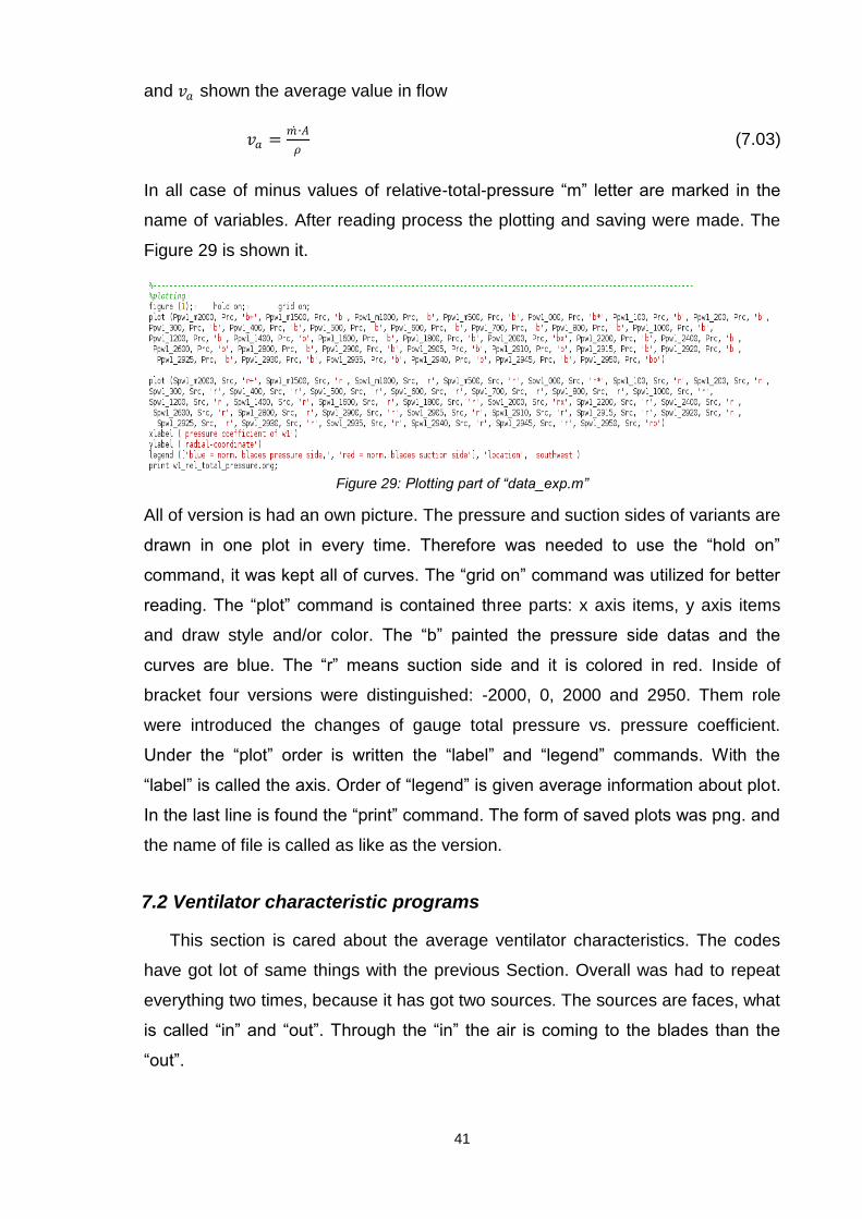
Figure 29: Plotting part of “data_exp.m”
All of version is had an own picture. The pressure and suction sides of variants are
drawn in one plot in every time. Therefore was needed to use the “hold on”
command, it was kept all of curves. The “grid on” command was utilized for better
reading. The “plot” command is contained three parts: x axis items, y axis items
and draw style and/or color. The “b” painted the pressure side datas and the
curves are blue. The “r” means suction side and it is colored in red. Inside of
bracket four versions were distinguished: -2000, 0, 2000 and 2950. Them role
were introduced the changes of gauge total pressure vs. pressure coefficient.
Under the “plot” order is written the “label” and “legend” commands. With the
“label” is called the axis. Order of “legend” is given average information about plot.
In the last line is found the “print” command. The form of saved plots was png. and
the name of file is called as like as the version.
7.2 Ventilator characteristic programs
This section is cared about the average ventilator characteristics. The codes
have got lot of same things with the previous Section. Overall was had to repeat
everything two times, because it has got two sources. The sources are faces, what
is called “in” and “out”. Through the “in” the air is coming to the blades than the
“out”.

42
Figure 30: Surface integral report in the inlet
Figure 31: Surface integral report in the outlet
At first the exports were done from Fluent. Figures 30 and 31 are shown us the
evaluator codes. The first line is not let to overwrite the older files that are means
the newer files datas are written after the older items. In all case “read and case”
code was used. After the reading, there is found the report orders. In first column
is contained the navigation orders. End of navigation is written mwa and meaning
of it is mass-weighted average. It was used in every time except the mass flow
exporting. From both iso-surfaces was taken the real-total-pressure and real-total-
temperature. Beside of them the density was written out from inlet. For the next
the mass flow rate and density was the same in the inlet and outlet, because the
working medium is air. Additional the real-total values some velocities were
copied. These were real-velocity-magnitude, real-tangential-velocity, and axial-
velocity. Because of the two surface in the “.out” it is needed to separate. The inlet
files are got „i‟ letter, and outlets are “o” e.g.: i_w1_-2000.out. The results of
exports are shown in Figure 32 and Figure 33. Unfortunately this “out.” files have
different structures than the previous Section. Therefore it was needed to use
another files for analyze the datas. This is shown in Figure 34, which is looked like
a block structure (matrix). These files are grouped in the original version
classification.

43
Figure 32: Reported data from inlet
Figure 33: Reported data from outlet

44
Figure 34: Reported datas in handing form
After manually grouping “io_program.m” is operated with these datas.
The preparation of the code is denoted in Figure 35. It is written with the same
block system like in “data_exp.m”. The first block commands are also the same,
but the auxiliary values are different. Values of range of “dlmread” are marked with
B and F. They indicate the lowest and highest row in matrix.
The other values need for calculation block. “BETA” equal with outlet angle (𝛽2),
and “Phi” is 𝜋. The revolution is n what was given in rad/min, because in practice
we use this dimension. In the program I prefer the angular velocity what marked in
rad/s. “Dou” is equal with the is defined 𝐷2., and “A” is the area of outlet (𝐴2).Value
of “U2” is the outlet wind speed (𝑣2). “I” and “O” letter are aggregated the inlet and
outlet datas. The numbers are shown the type of variation inside of the values.
Meaning of “rtp” is relative-total pressure, “d” is density, and “m1” is massflow in
the inlet. From the outlet it is cut the relative-total-pressure, relative velocity

45
magnitude, and relative tangential velocity, what are point “rtp”, “rvm”, “rtv” and
“ax”.
.
Figure 35: Reading of “io_program.m”
The first row of calculation is the flow coefficient calculation, what looks like in
normal way:
𝜑 =𝑚
𝜌∙𝜋∙𝜔∙𝐷23 (7.4)
In the next is cared to calculate the slip factor that marked “X”. At first it had to get
the value of “ALFA” (𝛼2)
𝛼2 =𝑣𝑅 ∙180
𝜋 (7.5)
where “vR” is the velocity ratio (𝑣𝑅):

46
𝑣𝑅 = sin−1 𝑣𝑟−𝑡𝑔 𝑣𝑟−𝑚𝑎𝑔 (7.6)
From Equations (6.4) and (6.5) we can calculate the slip factor
𝑋 = 180 − 𝛽2 − 𝛼2 (7.7)
Part of pressure coefficient calculation is had basic lows from Equations 5.50,
5.51, and 5.52. The sign of pressure coefficient is “fc” (𝜓), and calculated by.
𝜓 =2∙∆𝑝
𝜌∙ 𝜔∙𝐷2 2 (7.8)
In the last the efficiencies are made. We were calculated with pressure and
temperature efficiencies. For solve them it was needed to took the moment values.
At Figure 36 is shown one part of “exp_moment.jou” file.
Figure 36: Moment export file
After the reading commands is seen, that it was had to add new monitor to code.
This monitor is just written out the “moment cm” datas. In the middle of it was
located the place to setup the center of moment and direction. It is set in the origo
to z direction. In the end of it was needed to run some more calculation to got
datas. They are written into the “moment1.out” file. For better reading the datas
was separated by the versions. One of result of program is shown in Figure 37.
The first column is introduced the number of iterations of version, and in the
second there are the values of moment. In the Figure 35 is seen the values of
moment had to be calculate in the absolute form, because “negative moment” is

47
made “negative coefficient”, but all of coefficient have to be between 0 and 1
value.
Figure 37: Example about evaluated moment datas
Now with the moment is possible to calculi efficiencies. The shape of pressure
efficient is written:
𝜂 𝑝 =∆𝑝∙𝑚 1
𝑀𝑖 ∙𝜌1∙𝜔∙𝜅 (7.9)
where ∆𝑝 is the relative-total-pressure losses from Equation 7.2, 𝑚 1 is the mass
flow rate, 𝑀𝑖 is the moment of version values, 𝜌1 is the inlet density, ω angular
velocity, and κ is a constant (κ = 1.225/2). In the previous was determined, that
𝑚 1 = 𝑚 2, and 𝜌1 ≅ 𝜌2, because of the material conditions. The temperature
efficiency is not the same like pressure efficiency. The endpoint of calculation is
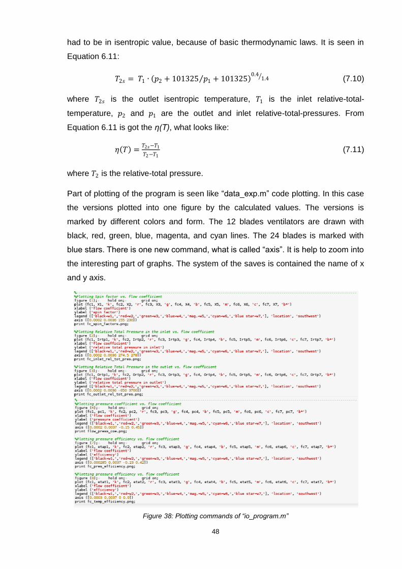
48
had to be in isentropic value, because of basic thermodynamic laws. It is seen in
Equation 6.11:
𝑇2𝑠 = 𝑇1 ∙ 𝑝2 + 101325 𝑝1 + 101325 0.4
1.4 (7.10)
where 𝑇2𝑠 is the outlet isentropic temperature, 𝑇1 is the inlet relative-total-
temperature, 𝑝2 and 𝑝1 are the outlet and inlet relative-total-pressures. From
Equation 6.11 is got the η(T), what looks like:
𝜂 𝑇 =𝑇2𝑠−𝑇1
𝑇2−𝑇1 (7.11)
where 𝑇2 is the relative-total pressure.
Part of plotting of the program is seen like “data_exp.m” code plotting. In this case
the versions plotted into one figure by the calculated values. The versions is
marked by different colors and form. The 12 blades ventilators are drawn with
black, red, green, blue, magenta, and cyan lines. The 24 blades is marked with
blue stars. There is one new command, what is called “axis”. It is help to zoom into
the interesting part of graphs. The system of the saves is contained the name of x
and y axis.
Figure 38: Plotting commands of “io_program.m”

49
8. DATA EVALUATION
In the Section 7 was seen how to got information for the ventilator
characteristics. This section aim is to give more information about version and
decide which one is better to use in out preferences.
8.1 Slip factor
Because of better understand it should be used this definition: Even under
ideal (frictionless) conditions the impeller of a ventilator will receive less then
perfect guidance from the vanes and the flow is said to slip. If the impeller could be
imagined as being made with an infinite number if infinitesimally thin vanes, then
an ideal flow would be perfectly guided by the vanes and would leave the impeller
at the angle [17]. It is seen in Equation 7.5, 7.6, and 7.7, how can calculate the slip
factor. Figure 39 is shown the slip factor vs. flow coefficient.
Figure 39: Slip factor vs. flow coefficient
In graph values of spin factors are changed between 0 and 100. With all of flow
coefficient it realized that the w1, w2, w3 are had got the biggest factors. It means
they have got the biggest looses. The w4 has got the smallest looses. w5, w6 and
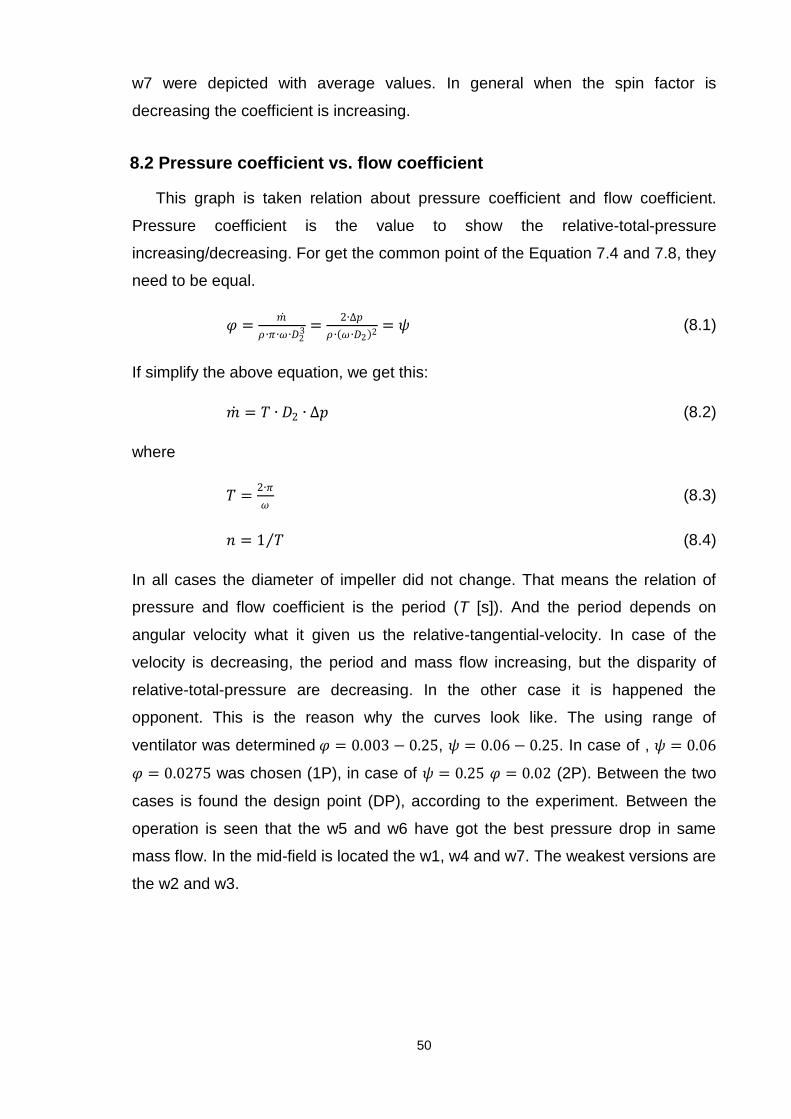
50
w7 were depicted with average values. In general when the spin factor is
decreasing the coefficient is increasing.
8.2 Pressure coefficient vs. flow coefficient
This graph is taken relation about pressure coefficient and flow coefficient.
Pressure coefficient is the value to show the relative-total-pressure
increasing/decreasing. For get the common point of the Equation 7.4 and 7.8, they
need to be equal.
𝜑 =𝑚
𝜌∙𝜋∙𝜔∙𝐷23 =
2∙∆𝑝
𝜌∙ 𝜔∙𝐷2 2= 𝜓 (8.1)
If simplify the above equation, we get this:
𝑚 = 𝑇 ∙ 𝐷2 ∙ ∆𝑝 (8.2)
where
𝑇 =2∙𝜋
𝜔 (8.3)
𝑛 = 1 𝑇 (8.4)
In all cases the diameter of impeller did not change. That means the relation of
pressure and flow coefficient is the period (T [s]). And the period depends on
angular velocity what it given us the relative-tangential-velocity. In case of the
velocity is decreasing, the period and mass flow increasing, but the disparity of
relative-total-pressure are decreasing. In the other case it is happened the
opponent. This is the reason why the curves look like. The using range of
ventilator was determined 𝜑 = 0.003 − 0.25, 𝜓 = 0.06 − 0.25. In case of , 𝜓 = 0.06
𝜑 = 0.0275 was chosen (1P), in case of 𝜓 = 0.25 𝜑 = 0.02 (2P). Between the two
cases is found the design point (DP), according to the experiment. Between the
operation is seen that the w5 and w6 have got the best pressure drop in same
mass flow. In the mid-field is located the w1, w4 and w7. The weakest versions are
the w2 and w3.
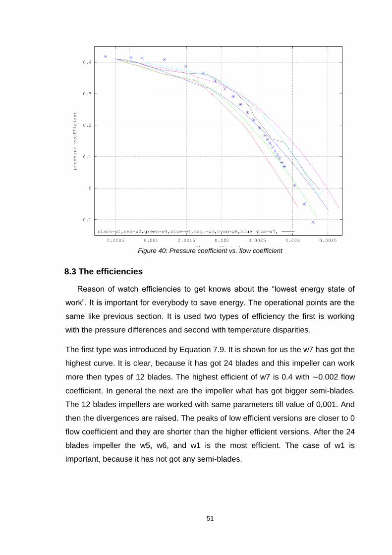
51
Figure 40: Pressure coefficient vs. flow coefficient
8.3 The efficiencies
Reason of watch efficiencies to get knows about the “lowest energy state of
work”. It is important for everybody to save energy. The operational points are the
same like previous section. It is used two types of efficiency the first is working
with the pressure differences and second with temperature disparities.
The first type was introduced by Equation 7.9. It is shown for us the w7 has got the
highest curve. It is clear, because it has got 24 blades and this impeller can work
more then types of 12 blades. The highest efficient of w7 is 0.4 with ~0.002 flow
coefficient. In general the next are the impeller what has got bigger semi-blades.
The 12 blades impellers are worked with same parameters till value of 0,001. And
then the divergences are raised. The peaks of low efficient versions are closer to 0
flow coefficient and they are shorter than the higher efficient versions. After the 24
blades impeller the w5, w6, and w1 is the most efficient. The case of w1 is
important, because it has not got any semi-blades.
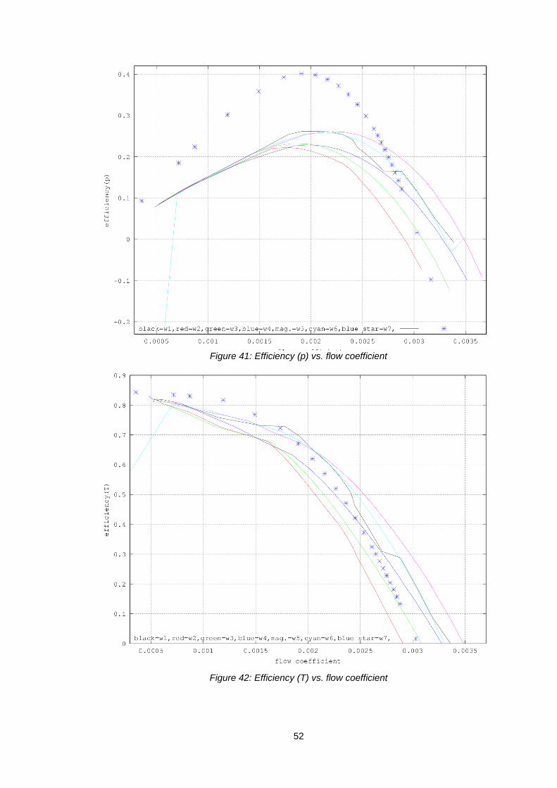
52
Figure 41: Efficiency (p) vs. flow coefficient
Figure 42: Efficiency (T) vs. flow coefficient

53
The efficiency what is made by temperature looks different. The curves have got
peaks. but they are located to far from operation points. The most same thing with
η (p) is the weakest versions still are w2, w3 and w4. Before them the w7 is
located. Above the operation range the w7 much better than the other. After the
range is produced one of the worst efficient. The w5 w6 and w1 behaving like the
previous, but w1 has got higher gradient than w5 and w6.
8.4 Relative-total pressure vs. flow coefficient
Figure 43: Relative-total-pressure vs. flow coefficient
It is shown in the previous that the pressure differences are one of the most
important items. Higher value of difference could be reach when the relative-total
pressure in the outlet is much more then inlet. Figure 43 and 44 are shown us
version on by one.
Inlet datas are had seen in Figure 43. Inside of working range the values are
depicted between 277 and 277.75 Pa. Disparity between versions less than 0.02-
0.03 Pa. That means to get higher pressure coefficient, it needed increase the
outlets relative-total-pressure.

54
Values of relative-total pressure are shown in Figure 44. Inside of process range
are huge numbers and changing of numbers, e.g.: in case of w2 the pressure
difference is nearby 1000 Pa. But it does not matter because inside of range the
functions of versions are linear.
Figure 44: Relative-total-pressure vs. flow coefficient
8.5 Radial coordinates vs. pressure coefficient
In Section 7.1 was introduced how the data export was worked one version. In
this part the results are shown. I wrote that the red curves are the part of suction
side, and blue curves are part of pressure side. And four sets was discriminated
from the others. In the part of suction lines can be realized one big brake, it is
called flow separation. The flow separation can be dangerous when the boundary
layer separation are made shedding vortex (Kármán Vortex Street). These vortex
have a chance to cause vibrations, and then make structural failures by the same
of resonance frequency. Therefore it is needed to investigate each version.
In case of w1 the separation is started at ~0.138 till .0162 m. Inside this the
pressure zone difference is ~ 1500 [Pa]. It is hold until 1000. After it the curves is
got more straight. Case of w2 is similar with w1 but the differences is reduced to

55
1000 [Pa]. Difference values of w3 sets is nearby 2000 [Pa] and it is hold till 2000
GTP. Range of drag is 0.024m. Separation of w4 it is begun at 0.135 m and it
finished at 0.16 m. The drop is ~2400 Pa. In the w5 the drop is 2500 Pa from 0.14
until 0.18. In case of w6 the separation is started at 0.135 till 0.175. The pressure
zone difference is ~2500 Pa. In the last case the drag is nearby 2500 Pa and
range is 0.045 m .
Figure 45: Radial coordinate vs. pressure coefficient of w1 and w2
Figure 46: Radial coordinate vs. pressure coefficient of w3 and w4
Figure 47: Radial coordinate vs. pressure coefficient of w5 and w6

56
Figure48: Radial coordinate vs. pressure coefficient of w7
Overall the flow separation depicted until 1400 GTP then the curves is begun
smooth. Before it the highest separation is with -2000 GTP every time. The
separation is started in 0.135 m and finished at 0.18 m. Range of it are not the
same. The first four versions have got 0.024-0.025 m distance between the
separation points. The last three have got 0.4- 0.45 m range. The pressure
coefficient zone is small in the beginning and later it is increasing.

57
9. ABSTRACT
In Section 8 the characteristics was shown. The most of the version are had
similar curves. From the choosing w1, w2, w3 fall out because of the weak
efficiencies. In the last four type the preferences do not change radically. But in the
flow separation graphs is seen the w4 has got less drag and range than the
others. At real-total-pressure figure is depicted, the w4 has got less difference
between the pressures (and in Figure 39). That means in the in the pressure
coefficient vs. flow coefficient picture the design point is lower than the others. And
w4 process with more air with the same efficiency.

58
10. ACKNOWLEDGEMENT
I was very pleased that I learned a whole year in Czech Republic by
ERASMUS program. I would like to thank all those people who contributed to my
studies at home and aboard. Special thanks to my tutor Ing. Roman Gaspar PhD
Student, and Doc. Ing. Jiri Polansky Ph.D the Head of Department of Power
System Engineering, who gave advices and helped in troubles.
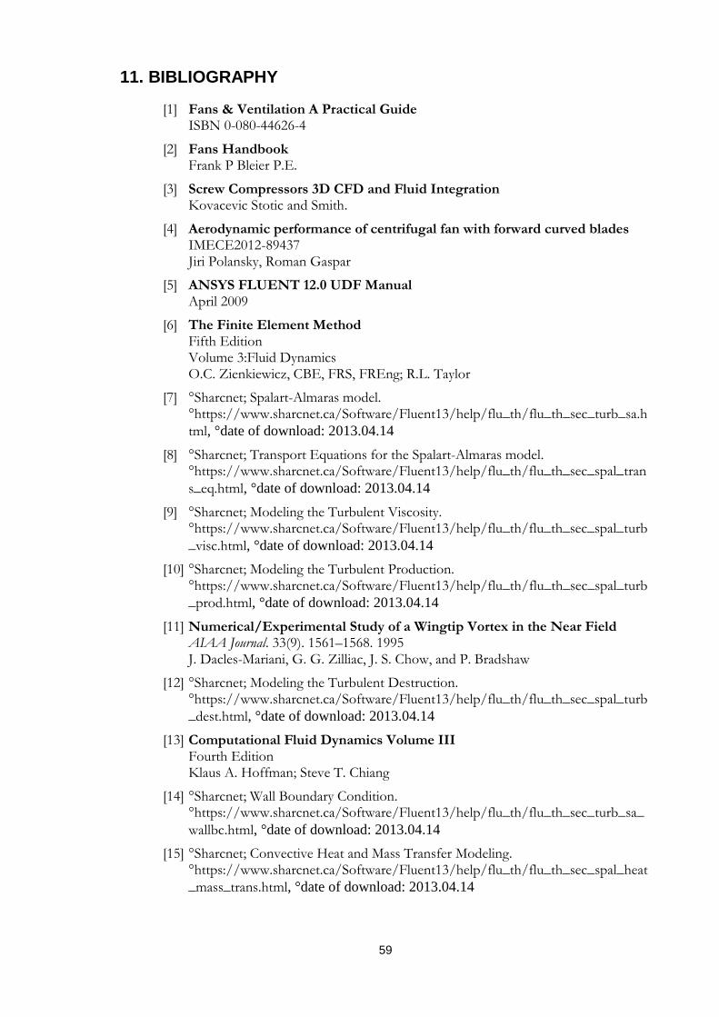
59
11. BIBLIOGRAPHY
[1] Fans & Ventilation A Practical Guide ISBN 0-080-44626-4
[2] Fans Handbook Frank P Bleier P.E.
[3] Screw Compressors 3D CFD and Fluid Integration Kovacevic Stotic and Smith.
[4] Aerodynamic performance of centrifugal fan with forward curved blades IMECE2012-89437 Jiri Polansky, Roman Gaspar
[5] ANSYS FLUENT 12.0 UDF Manual April 2009
[6] The Finite Element Method Fifth Edition Volume 3:Fluid Dynamics O.C. Zienkiewicz, CBE, FRS, FREng; R.L. Taylor
[7] °Sharcnet; Spalart-Almaras model. °https://www.sharcnet.ca/Software/Fluent13/help/flu_th/flu_th_sec_turb_sa.h
tml, °date of download: 2013.04.14
[8] °Sharcnet; Transport Equations for the Spalart-Almaras model. °https://www.sharcnet.ca/Software/Fluent13/help/flu_th/flu_th_sec_spal_tran
s_eq.html, °date of download: 2013.04.14
[9] °Sharcnet; Modeling the Turbulent Viscosity. °https://www.sharcnet.ca/Software/Fluent13/help/flu_th/flu_th_sec_spal_turb
_visc.html, °date of download: 2013.04.14
[10] °Sharcnet; Modeling the Turbulent Production. °https://www.sharcnet.ca/Software/Fluent13/help/flu_th/flu_th_sec_spal_turb
_prod.html, °date of download: 2013.04.14
[11] Numerical/Experimental Study of a Wingtip Vortex in the Near Field AIAA Journal. 33(9). 1561–1568. 1995 J. Dacles-Mariani, G. G. Zilliac, J. S. Chow, and P. Bradshaw
[12] °Sharcnet; Modeling the Turbulent Destruction. °https://www.sharcnet.ca/Software/Fluent13/help/flu_th/flu_th_sec_spal_turb
_dest.html, °date of download: 2013.04.14
[13] Computational Fluid Dynamics Volume III Fourth Edition Klaus A. Hoffman; Steve T. Chiang
[14] °Sharcnet; Wall Boundary Condition. °https://www.sharcnet.ca/Software/Fluent13/help/flu_th/flu_th_sec_turb_sa_
wallbc.html, °date of download: 2013.04.14
[15] °Sharcnet; Convective Heat and Mass Transfer Modeling. °https://www.sharcnet.ca/Software/Fluent13/help/flu_th/flu_th_sec_spal_heat
_mass_trans.html, °date of download: 2013.04.14

60
[16] °Sharcnet; The Energy Transport Equation. °https://www.sharcnet.ca/Software/Fluent13/help/flu_th/flu_th_sec_hxfer_the
ory.html#x1-2210006.2.1, °date of download: 2013.04.14
[17] GNU Octave Free Your Numbers John W. Eaton, David Bateman, Søren Hauberg
[18] Turbo Mehcanics and Thermodynamics of Turbomachinery Fifth Edition S. L. Dixon