
Numerical Investigation of Flow Induced Noise in a ...652385/FULLTEXT01.pdfNumerical Investigation...
114
Numerical Investigation of Flow Induced Noise in a Simplified HVAC Duct with OpenFOAM CONG WANG Master Thesis Stockholm, Sweden 2013
-
Upload
duongtuyen -
Category
Documents
-
view
222 -
download
2
Transcript of Numerical Investigation of Flow Induced Noise in a ...652385/FULLTEXT01.pdfNumerical Investigation...
Numerical Investigation of Flow Induced Noise in a Simplified HVAC
Duct with OpenFOAM
CONG WANG
Master Thesis Stockholm, Sweden 2013

i
Preface
The work presented in this thesis has been carried out at the Department of
Performance Engineering in Bombardier Transportation. Aero-acoustic research has
been a hot topic in recent years in both academic community and industrial world. In
this research, the flow induced noise in a simplified HVAC duct has been numerically
investigated. The feasibility of a hybrid method in computational aero-acoustics has
been studied.
First and foremost, I would like to express my sincere gratitude towards my three
supervisors from Bombardier Transportation. They are Erik Wik, Karl-Richard Kirchner,
and Fabian Brännström. Erik interviewed me and arranged everything for me such as
office, transportation and accommodation. Richard conducted acoustic computation,
the result of which verifies the CFD simulation. Special thanks to Fabian, who always
provided me with valuable suggestions and instructions in the whole work. I have
learnt quite a lot from you in both fluid dynamics and work style.
I am very grateful to my KTH supervisors Prof. Arthur Rizzi and Prof. Jesper
Oppelstrup for all the great support and feedback provided. It has been a great
pleasure to work under the supervision of Prof. Rizzi. I want to thank Prof. Oppelstrup
for the detailed and useful suggestions and comments.
I would like to thank all my colleagues at the group of Aero- and Thermodynamics for
their sincere help. Working with you has been a great experience.
Last but not least, I am deeply indebted to my parents for their continuous support
and generous love for all of these years.

iii
Abstract
Due to the growing demand for comfort, the noise generated by HVAC components
should be considered by the designers. Flow induced noise is one of the major
contributors to the noise in HVAC systems. By means of computational aero-acoustics
(CAA), the mechanism of noise generation is able to be studied in the design phase.
This research has been conducted based on a simplified HVAC duct, aiming to
validate a hybrid method in CAA. The hybrid method is an affordable and promising
approach for industrial applications. CFD simulation, as the first step of the hybrid
method, has been performed. Due to the deficiency of RANS and high computational
cost of LES, hybrid RANS-LES approaches are employed to combine sufficient
accuracy and reduced cost. Delayed Detached Eddy Simulation (DDES) and Scale
Adaptive Simulation (SAS), as the representative hybrid RANS-LES approaches, are
performed and compared. CFD results are shown in detail and compared with the
experimental measurements available in the literature. The comparison shows a
good agreement for the time averaged flow field and a fairly good agreement for
unsteady flow phenomena. Discrepancies between numerical results and
measurements can be observed regarding mainly unsteady pressure fluctuations.
The influence study of grid, discretization schemes, time step as well as other
parameters is also conducted. The insights gained here can serve as a guideline for
future complex applications.

v
Table of Contents
Preface ............................................................................................................................ i
Abstract ......................................................................................................................... iii
List of Figures ............................................................................................................... vii
List of Tables .................................................................................................................. ix
Nomenclature ............................................................................................................... xi
1. Introduction ............................................................................................................ 1
1.1 Importance of Acoustic Research ................................................................. 1
1.2 Introduction to CAA ...................................................................................... 2
1.3 Introduction to the Test Case ....................................................................... 5
1.4 Outline .......................................................................................................... 5
2. Theoretical Background .......................................................................................... 6
2.1 Flow Physics and Turbulence Modeling ....................................................... 6
2.1.1 Governing Equations .......................................................................... 6
2.1.2 Reynolds Averaged Navier-Stokes Simulation ................................... 8
2.1.3 Large Eddy Simulation ...................................................................... 13
2.1.4 Hybrid RANS-LES Simulation ............................................................ 16
2.2 Computational Fluid Dynamics and OpenFOAM ........................................ 21
2.2.1 Overview .......................................................................................... 21
2.2.2 OpenFOAM....................................................................................... 23
2.2.3 Finite Volume Discretization ............................................................ 25
2.2.4 Solution ............................................................................................ 34
3. Cases and Results .................................................................................................. 40
3.1 Test Case Description .................................................................................. 40
3.1.1 Geometry – Simplified HVAC duct ................................................... 40
3.1.2 Experimental Rig .............................................................................. 41
3.1.3 Related Numerical Studies ............................................................... 43
3.2 Numerical Simulation ................................................................................. 45
3.2.1 Computational Domain .................................................................... 45
vi
3.2.2 Meshing ............................................................................................ 46
3.2.3 Boundary Conditions ....................................................................... 48
3.2.4 Hybrid RANS-LES Approaches .......................................................... 51
3.2.5 Simulation Details ............................................................................ 53
3.3 Results and Comparisons ........................................................................... 58
3.3.1 Unsteady Pressure Fluctuations ....................................................... 58
3.3.2 Time Averaged Flow Field ................................................................ 64
3.3.3 Influence Study ................................................................................ 70
3.3.4 Discussions ....................................................................................... 75
4. Conclusions and Recommendations ..................................................................... 79
4.1 Conclusions ................................................................................................. 79
4.2 Recommendations ...................................................................................... 80
Bibliography ................................................................................................................. 83
Appendix A ................................................................................................................... 86
Appendix B ................................................................................................................... 88
Appendix C ................................................................................................................... 90
Appendix D ................................................................................................................... 93
Appendix E ................................................................................................................... 94
Appendix F ................................................................................................................... 95
Appendix G ................................................................................................................... 97

vii
List of Figures
Figure 1-1: Overview of CAA conceptual approaches. .......................................... 4
Figure 2-1: Clear (left) and ambiguous (right) DES grid ....................................... 18
Figure 2-2: Overview of the structure and content of an OpenFOAM case ........ 24
Figure 2-3: Control Volume in Finite Volume Method ......................................... 26
Figure 2-4: Over-relaxed decomposition approach. ............................................ 30
Figure 3-1: Geometry of the simplified HVAC duct .............................................. 41
Figure 3-2: Experimental Setup ............................................................................ 42
Figure 3-3: Locations of 7 microphones ............................................................... 43
Figure 3-4: PIV and acoustic measurement setup ............................................... 43
Figure 3-5: Geometry of the computational domain. .......................................... 46
Figure 3-6: Two grids with local refinements ....................................................... 47
Figure 3-7: Overview of boundary conditions ..................................................... 48
Figure 3-8: Sound Pressure Level at 7 microphone locations of DDES-G1. ......... 61
Figure 3-9: Sound Pressure Level at 7 microphone locations of DDES-G2. ......... 61
Figure 3-10: Sound Pressure Level at 7 microphone locations of SAS-G1. .......... 61
Figure 3-11: SPL Comparisons of simulations and experiment. .......................... 63
Figure 3-12: Simulated time averaged velocity magnitude in section y=0. ......... 64
Figure 3-13: Simulated time averaged velocity components in section y=0 ....... 65
Figure 3-14: Experimental time averaged velocity components in section y=0 .. 65
Figure 3-15: Simulated projected velocity vector in section y=0. ........................ 66
Figure 3-16: Experimental projected velocity vector in section y=0 ................... 66
Figure 3-17: Close up view of simulated projected velocity vectors ................... 67
Figure 3-18: Close up view of experimental projected velocity vectors. ............. 67
Figure 3-19: Mean and r.m.s. value of pressure at walls ..................................... 69
Figure 3-20: Comparison of convective discretization schemes. ......................... 73
Figure 3-21: Comparison of laplacian discretization schemes............................. 73
Figure 3-22: Comparison of time steps based on DDES-G1 ................................. 74
Figure 3-23: Comparison of two time steps based on SAS-G1 ............................ 74

viii
Figure 3-24: Instantaneous z-component of vorticity in section y=0. ................. 75
Figure 3-25: Iso-contour of Q = 3E+4 colored by velocity magnitude ................. 78
ix
List of Tables
Table 3-1: Overview of parameters of the two grids ........................................... 48
Table 3-2: Boundary conditions for pressure and velocity. .................................. 50
Table 3-3: Description and names of simulation cases. ....................................... 51
Table 3-4: Boundary conditions for turbulence variables. ................................... 53
Table 3-5: Overview of the spacial and temporal discretization schemes. .......... 55
Table 3-6: Setup of the transient SIMPLE algorithm. ........................................... 56
Table 3-7: Setup of the solvers for linear algebraic equations. ........................... 56
Table 3-8: Performance of the numerical simulations. ........................................ 57
Table 3-9: Mean pressure at seven microphone locations. ................................. 59
Table 3-10: Variance of the pressure signasl at seven microphone locations. .... 59
Table 3-11: Parameters for frequency analysis. ................................................... 60
Table 3-12: Selection for laplacian discretization schemes. ................................ 71

xi
Nomenclature
Abbreviations
B.C. Boundary Condition
BD Backward Differencing
CAA Computational Aero-acoustics
CD Central Differencing
CFD Computational Fluid Dynamics
CFL Courant number
CV Control Volume
DDES Delayed Detached Eddy Simulation
DES Detached Eddy Simulation
DNS Direct Numerical Simulation
FV Finite Volume
FW-H Fowcs-Williams Hawkings
GAMG Geometric Algebraic Multi-Grid solver
GIS Grid Induced Separation
LEE Linearized Euler Equations
LES Large Eddy Simulation
LES-NWM Large Eddy Simulation with near-wall modeling
LES-NWR Large Eddy Simulation with near-wall resolution
LUD Linear Upwind Differencing
LUST Linear Upwind Stabilized Transport
MSD Modeled Stress Depletion
PISO Pressure Implicit with Splitting of Operators
PIV Particle Image Velocimetry
PSD Power Spectra Density
RANS Reynolds Averaged Navier-Stokes
r.m.s. root-mea- square
xii
SAS Scale Adaptive Simulation
SGS Sub Grid Scale
S-A Spalart-Allmaras
SIMPLE Semi-Implicit Method for Pressure-Linked Equations
SPL Sound Pressure Level
SST Shear Stress Transport
STL Stereolithography
Roman
hydraulic diameter
nearest wall distance
modified nearest wall distance
distance vector between and
total specific energy
mass flux through the face
face, centroid of the face
external body force vector
( ) LES filter function
transport part
turbulence intensity
turbulent kinetic energy
residual (SGS) kinetic energy
turbulence mixing length
center of the neighboring control volume
center of the control volume
instantaneous pressur e
filtered pressure
total pressure
xiii
⟨ ⟩ mean pressure
filtered pressure
reference sound pressure
Q second invariant of velocity gradient tensor
heat flux vector
Reynolds number
distance vector between cell center and face centroid
mean rate-of-strain tensor
filtered rate-of-strain
face area vector
orthogonal part of face area vector
non-orthogonal part of face area vector
velocity field
( ) instantaneous velocity field
( ) filtered velocity field
( ) residual velocity field
fluctuating velocity component
control volume
distance in wall unit
Greek
matrix coefficient corresponding to the cell N
central coefficient
pressure under-relaxation factor
velocity under-relaxation factor
grid space
filter width
Kronecker delta
xiv
turbulence dissipation rate
dynamic viscosity
kinematic viscosity
effective kinetic viscosity
residual (SGS) eddy viscosity (LES)
SGS eddy viscosity
turbulent viscosity (RANS)
turbulent viscosity
modified turbulent viscosity
density
general scalar property
magnitude of mean voticity
specific dissipation rate
Super- and Sub-script
fluctuating component
filtered quantity
value on the face
Symbols
⟨ ⟩ mean operator
( ) face value
gradient operator
divergence operator
first cell center thickness
frequency resolution

1
1. Introduction
1.1 Importance of Acoustic Research
Acoustics, which has both positive and negative sides, has significantly affected our
daily lives. Pleasant music and sound have good effects on our health, which is the
positive side. The negative side of acoustics is the so called noise. It has been shown
that noise can have negative impact on health, activity and even annoyance [1].
Noise can be generated by several physical interaction mechanisms: solid body
friction, solid body vibration, combustion, and aerodynamic noise [1]. Aerodynamic
noise is also referred to as aero-acoustics, flow induced noise or flow acoustics.
There are slight differences between these terms, but they are not distinguished in
this thesis. Similarly, the terms like sound, noise and acoustics are interchangeably
used in this thesis.
Heating, Ventilation and Air Conditioning (HVAC) system is designed to regulate
temperature and maintain good in-door air quality. One important part of noise
generation in HVAC system is the power unit, which often emits tonal noise at a
constant frequency that is transported through the duct system. Besides this, flow
induced noise is caused by obstacles within the ducts. Despite the relatively low
noise level of HVAC systems, it is annoying and due to the growing customers’
demand as well as legal requirement it should be considered by the designers.
In this thesis, the focus has been put on the noise generated by HVAC system. The
main purpose of this work is to validate the feasibility of a hybrid method in
Computational Aero-acoustics (CAA) to correctly predict the noise in the HVAC
system. The noise generated by the blower, for simplicity, is not considered.
2
1.2 Introduction to CAA
Aero-acoustics considers sound generated by aerodynamic forces or motions
originating from turbulent flows. Aero-acoustic research dates back to James Lighthill
who in the early 1950’s firstly represented the sound as the difference between the
actual flow and a reference flow. He developed the foundation of aero-acoustics –
acoustic analogy, by rewriting the Navier-Stokes equations in a way that the
equivalent aero-acoustic sources can be defined. Since then, this acoustics analogy
had been widely used and extended to incorporate the influence of a solid boundary
(Curle’s analogy) and surfaces in arbitrary motions (FW-H method).
Advances in computational power have made it possible to use the numerical
approaches in acoustic research. A new subject - Computational Aero-acoustics (CAA)
therefore arises.
Despite the large number of CAA approaches that exist nowadays, one can clearly
distinguish two groups of approaches [1]:
Direct methods literally mean to compute the acoustic field directly. The flow fields
and the acoustic field area computed together at the same time. The compressible
Euler or Navier-Stokes equations are solved in the domain from the aerodynamics
area down to the far field observer. Direct methods are comparable to the Direct
Numerical Simulation (DNS) in the Computational Fluid Dynamics (CFD) and are
considered as the most accurate approach. However, they are not commonly used in
industrial applications, because of the following disadvantages:
Extremely high computational cost. The computational cost of 3-D DNS scales with
the cubic of the Reynolds number, which prohibits the industrial applications.
Inherent multi-scale problems. Acoustic motion in general has a much smaller order
3
than the aerodynamic motion. This large disparity prevents the use of direct
methods. If not taken care of appropriately, the acoustic solution may be totally
polluted by computational noise.
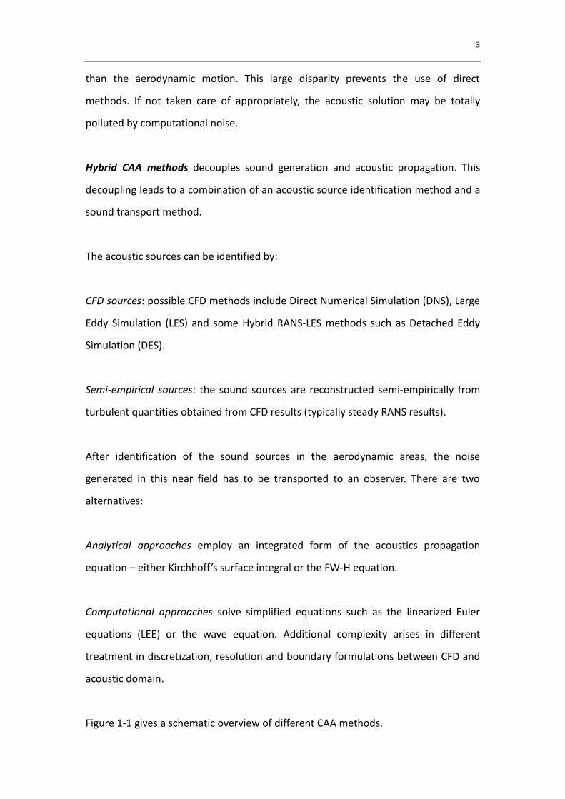
Hybrid CAA methods decouples sound generation and acoustic propagation. This
decoupling leads to a combination of an acoustic source identification method and a
sound transport method.
The acoustic sources can be identified by:
CFD sources: possible CFD methods include Direct Numerical Simulation (DNS), Large
Eddy Simulation (LES) and some Hybrid RANS-LES methods such as Detached Eddy
Simulation (DES).
Semi-empirical sources: the sound sources are reconstructed semi-empirically from
turbulent quantities obtained from CFD results (typically steady RANS results).
After identification of the sound sources in the aerodynamic areas, the noise
generated in this near field has to be transported to an observer. There are two
alternatives:
Analytical approaches employ an integrated form of the acoustics propagation
equation – either Kirchhoff’s surface integral or the FW-H equation.
Computational approaches solve simplified equations such as the linearized Euler
equations (LEE) or the wave equation. Additional complexity arises in different
treatment in discretization, resolution and boundary formulations between CFD and
acoustic domain.
Figure 1-1 gives a schematic overview of different CAA methods.
4
Figure 1-1: Overview of CAA conceptual approaches (Wagner et al. (2007) [1]).
5
1.3 Introduction to the Test Case
The purpose of this thesis is to investigate the feasibility of correctly predicting the
noise generated within HVAC systems by numerical simulations. To avoid
unpredictable and unknown difficulties and also to keep the meshing and
computational efforts minimal, the representation of the HVAC duct should be kept
as simple as possible. However, important characteristic elements of a real HVAC
duct have to be included in order for us to gain an insight into the aero-acoustic
mechanism. Two important characteristics are pressure driven flow separation and
flow around an obstacle. The test case in our study is a rectangular cross-section duct
with a 90 degree bend and a flap inside, representing two important characteristics:
pressure driven flow and flow around an obstacle.
In the previous section of this chapter, different CAA approaches have been
described. It is clear that the hybrid method, in which the flow field and acoustic field
are solved separately, could be the only appropriate and possible technique for this
study. CFD simulations are performed on two grids of different qualities. Two
different hybrid RANS-LES approaches are used in CFD simulation and compared with
each other. The influences of numerical setup are also studied.
1.4 Outline
The general outline of this thesis is given below. The first chapter presented here
gives a short introduction to the state of the art in computational aero-acoustics. The
second chapter focuses on the theoretical background, in which the flow physics,
mathematic modeling for turbulence, and numerical methods for CFD are described.
Chapter 3 presents a detailed description of the test case and shows the results and
comparisons with experimental measurements. Finally, the thesis is completed by
Chapter 4 with conclusions and recommendations.
6
2. Theoretical Background
This chapter presents the relevant theoretical background and is divided into two
sections. Section 2.1 briefly describes the flow physics as well as methodologies for
modeling turbulence. Section 2.2 gives an overview of the numerical approach – CFD
and the software OpenFOAM that is used in this work.
2.1 Flow Physics and Turbulence Modeling
In this section, the governing equations of fluid flows are firstly introduced in
subsection 2.1.1. The different approaches for turbulence modeling are then
described in next three subsections.
2.1.1 Governing Equations
The equations that govern the motions of Newtonian fluid are the Navier-Stokes
equations, which are the underlying principles of fluid dynamics. For a 3-dimensional,
unsteady and compressible flow, the full governing equations consist of five
equations. The first equation is the so called continuity equation, which describes the
conservation of mass. The next three represent the conservation of momentum in
three directions. The last equation formulates the conservation of energy. These
equations are presented in conservative form below:
𝜕𝜌
𝜕 + = 0 (2-1)
𝜕𝜌
𝜕 + ( ) = − + ( ) + (2-2)
𝜕𝜌
𝜕 + ( ) = − ( ) + ( ) + − (2-3)
where , , and are the pressure, density and total specific energy respectively.
Here is the dynamic viscosity of the fluid, is the external body force (e.g. the
gravity), and is the heat flux vector. The symbol named Nabla, refers to the
divergence operator defined as:
= (∂
∂𝑥
∂
∂𝑦
∂
∂𝑧) (2-4)

7
The number of unknown quantities in the above equations is 9 ( , , , , and 𝑞 ),
which is larger than the number of equations (1+3+1=5). Therefore more equations
describing constitutive relationships are necessary to close the equations.
When Mach number of the flow is low, the flow can be considered as incompressible,
resulting in a constant and homogeneous density throughout the flow field. If the
change of temperature in the flow is small, the influence of the temperature on the
flow field can be neglected. The last equation for the conservation of energy can
then be omitted. The governing equations for incompressible and isothermal flow
can be rewritten in a simpler form as follows:
= 0 (2-5)
𝜕
𝜕 + ( ) = − + ( ) (2-6)
where = is the kinematic viscosity. Now only four unknown quantities
remain, corresponding to four equations. The system is then closed.
Turbulence or turbulent flow may occur when the Reynolds number exceeds beyond
a critical value. The Reynolds number (Re) is a non-dimensional number generally
defined as the ratio of a characteristic velocity times a characteristic length to the
kinematic molecular viscosity. Turbulent flow is characterized by a random and
chaotic behavior of the flow. It contains rotational flow structures, the so called
turbulent eddies, which cause rapid change of velocity and pressure. These eddies
appear in a wide range of length and time scales. The length scales range from the
largest scales, which are of the order of the geometry, to the smallest scales - the
Kolmogorov scales. The kinematic energy of the largest scales, which extract energy
from the mean flow, is transferred to smaller scales. The energy is finally transferred
to the Kolmogorov scales and then dissipated. This process is referred to as the
8
energy cascade [2].
Aero-acoustics is inherently connected with the existence of turbulence. It is
necessary to take turbulence into account in order to simulate the flow correctly.
There are various ways of computing turbulence structures of different scales.
Direct Numerical Simulation solves the Navier–Stokes equations directly without
using any turbulence model. The whole range of spatial and temporal scales of the
turbulence is resolved. For a 3-dimentional flow simulation, the computational cost
of DNS scales approximately with 3[2]. Due to the highly demanding requirement
for the computational power as well as other difficulties such as special care for
discretization schemes and boundary conditions, it is almost impossible to be applied
to complex flows in industrial applications.
It is therefore necessary to employ turbulence models, which model the influence of
the turbulence to the flow. The Large Eddy Simulation (LES) and Reynolds Averaged
Navier-Stokes simulation (RANS) represent two basic kinds of simulation for
turbulent flows.
2.1.2 Reynolds Averaged Navier-Stokes Simulation
The Reynolds Averaged Navier-Stokes (RANS) equations is derived from the
instantaneous Navier-Stokes equations by means of Reynolds decomposition, which
separates the flow variables (e.g. velocity , pressure etc.) into a mean
component and a fluctuating component. Without loss of generality, for an arbitrary
flow quantity , the Reynolds decomposition reads:
= ⟨ ⟩ +
where ⟨ ⟩ is the mean value and is the fluctuating part. For unsteady RANS
(URANS), the mean value is often referred to as the ensemble average or phase
average in contrast to the time average in steady RANS. The mean operator ⟨ ⟩ is
9
called Reynolds operator and has a set of properties, one of which is that the mean
of the fluctuating part is equal to zero. To avoid confusion, the notation , ⟨ ⟩ and
will be used to represent the instantaneous, mean and fluctuating terms,
respectively.
After taking the mean of the Navier-Stokes equations, The RANS equations are
obtained, which are expressed in tensor notation as follows:
𝜕⟨ 𝑖⟩
𝜕𝑥𝑖= 0 (2-7)
𝜕⟨ 𝑖⟩
𝜕 +
𝜕⟨ 𝑖⟩⟨ 𝑗⟩
𝜕𝑥𝑗= −
1
𝜌
𝜕⟨ ⟩
𝜕𝑥𝑖+
𝜕2⟨ 𝑖⟩
𝜕𝑥𝑗𝜕𝑥𝑗−
𝜕⟨𝑢𝑖′𝑢𝑗
′⟩
𝜕𝑥𝑗 (2-8)
The left hand side of Eqn. (2-8) represents the change of mean momentum in a fluid
element owing to the unsteadiness in the mean flow and the convection by the
mean flow. This change is balanced by the right hand side, which includes the mean
pressure, the viscous stress and an extra source term −⟨
⟩ caused by the
fluctuating velocity field, generally referred to as the Reynolds stress.
It can be seen that the RANS equations have a similar form to the Navier–Stokes
equations, except the Reynolds stress term. This term raises the closure problem and
requires additional modeling. Analogous to the molecular viscosity which describes
the stress-rate-of-strain relation for a Newtonian fluid, the turbulent-viscosity
introduced by Boussinesq in 1877 links the Reynolds stress to the mean rate-of-strain.
According to the hypothesis, the deviatoic Reynolds stress is proportional to the
mean rate of strain [2]:
−⟨
⟩ +2
3 = (
𝜕⟨ 𝑖⟩
𝜕𝑥𝑗+
𝜕⟨ 𝑗⟩
𝜕𝑥𝑖) = 2 (2-9)
where the positive scalar coefficient is the turbulent viscosity (also called eddy
10
viscosity), is the mean rate-of-strain tensor, and is the turbulent kinetic
energy defined as half the trace of the Reynolds stress tensor ≡1
2⟨
⟩.
Substitution of Eqn. (2-9) into Eqn. (2-8) yields
𝜕⟨ 𝑖⟩
𝜕 +
𝜕⟨ 𝑖⟩⟨ 𝑗⟩
𝜕𝑥𝑗= −
1
𝜌
𝜕
𝜕𝑥𝑖⟨ ⟩ +
𝜕2⟨ 𝑖⟩
𝜕𝑥𝑗𝜕𝑥𝑗 (2-10)
where ( ) = + ( ) is the effective viscosity. Eqn. (2-10) is the same as
the Eqn. (2-8) with ⟨ ⟩ and in place of and , with ⟨ ⟩ ≡ ⟨ ⟩ +2
3 the
modified mean pressure.
However, the hypothesis raises a new quantity - turbulent viscosity , which has to
be determined. A couple of models have been proposed to determine the turbulent
viscosity. Depending on the number of transport equations solved, these models fall
into several groups: algebraic, one-equation, two-equation and Reynolds-stress
models. The Spalart-Allmaras model as a one-equation and the − 𝑇 model
as a two-equation model are briefly described in the following sections, since they
are involved later in the hybrid RANS-LES approaches.
The Spalart-Allmaras model
Spalart and Allmaras (1992) [3] described a one-equation model developed for the
aerodynamics applications, in which a single transport equation is solved for the
turbulent viscosity. The turbulent viscosity is defined by
= f𝑣1
with f𝑣1
=𝜒3
𝜒3 𝑐𝑣13 and 𝜒 =
��
𝜈
where 𝑐𝑣1 is a constant, is the molecular kinematic viscosity, and is the
11
modified eddy viscosity computed from the transport equation given by
𝜕��
𝜕 + ⟨𝑈 ⟩
𝜕��
𝜕𝑥𝑗= 𝑐𝑏1 +
1
𝑐𝜎[
𝜕
𝜕𝑥𝑗( + )
𝜕��
𝜕𝑥𝑗+ 𝑐𝑏2
𝜕��
𝜕𝑥𝑖
𝜕��
𝜕𝑥𝑖] − 𝑐w1fw (
��
𝑑) (2-11)
Additional definitions are given by the following expressions:
= +ν
𝜅2𝑑2f𝑣2
(2-12)
where is the magnitude of the mean vorticity, is the distance from the field
point to the nearest wall, and
f𝑣2
= 1 −𝜒
1 + 𝜒f𝑣1
fw
= 𝑔 [1 + 𝑐w3
6
𝑔6 + 𝑐w36 ]
𝑔 = 𝑟 + 𝑐w2(𝑟6 − 𝑟)
𝑟 = 𝑚𝑖𝑛 [
𝜅2 2 10]
Details regarding the model and the constants can be found in [3] and [4].
The 𝒌 − 𝝎 𝑻 model
Many two-equation models have been proposed. In most of these, the turbulent
kinetic energy is taken as one of the variables, but there are various choices for
the second. Examples are the most widely used − model, with the dissipation
rate being the second variable, and the − model solving the second
transport equation for the specific dissipation rate (also referred to as turbulent
frequency) ≡ .
Menter (1994) [5] proposed a two-equation model − 𝑇. 𝑇 represents the
shear stress transport formulation which combines the best behavior of the two
12
models. The use of a − formulation in the inner part of the boundary layers
makes the model directly usable all the way down to the wall through the viscous
sub-layer. The SST formulation also switches to a − behavior in the free-stream
and thereby avoids the common − problem that the model is too sensitive to
the inlet free-stream turbulence properties. The − 𝑇 model is merited by the
users for its good performance in adverse pressure gradients and separating flow [2].
Eqn. (2-13) and Eqn. (2-14) are the transport equations for and respectively,
𝜕𝑘
𝜕 + ⟨𝑈 ⟩
𝜕𝑘
𝜕𝑥𝑗= +
𝜕
𝜕𝑥𝑗[( + 𝜎𝑘 )
𝜕𝑘
𝜕𝑥𝑗] − 𝛽∗ (2-13)
𝜕𝜔
𝜕 + ⟨𝑈 ⟩
𝜕𝜔
𝜕𝑥𝑗=
𝛾
𝜈𝑇 +
𝜕
𝜕𝑥𝑗[( + 𝜎𝜔 )
𝜕𝑘
𝜕𝑥𝑗] − 𝛽 2 + 2(1 − 1)
𝜎𝜔2
𝜔
𝜕𝑘
𝜕𝑥𝑗
𝜕𝜔
𝜕𝑥𝑗 (2-14)
where = 2 represents the production of turbulent kinetic energy and the
turbulent viscosity is computed from
= 1
𝑚 𝑥( 1 2)
where is the magnitude of the mean vorticity (or rate of rotation), 2 depends
on , and the distance to the nearest wall .
Each of the model coefficients is a blend of two constants, blended via
= 1 + (1 − 1) 2
where 1represents constant 1 and 2represents constant 2. 1 is a function of ,
and .
Detailed information regarding formulation, variants and the values of constants can
be found in [5] and [6].
13
2.1.3 Large Eddy Simulation
In large eddy simulation (LES), the larger energy-containing unsteady turbulent
motions are directly solved, whereas the effects of the smaller-scale motions are
modeled. Since the larger-scale unsteady motions are represented explicitly, LES can
be expected to be more accurate and reliable than RANS for flows in which
large-scale unsteadiness is significant. Compared with RANS, the higher level of
description by LES increases its applicability to aero-acoustics and other phenomena
associated with unsteady turbulent motions [2].
As discussed in the previous chapter, the computational cost of DNS is high, and
increases with the cube of the Reynolds number, so that DNS is so far inapplicable to
high-Reynolds-number flows. Most of the computational time in DNS is spent on the
smallest, dissipative motions, whereas the energy and anisotropy are contained
predominantly in the larger-scale motions. In LES, the dynamics of the larger-scale
motions are computed explicitly, with the influence of the smaller scales being
modeled [2]. Thus compared with DNS, the vast computational cost of explicitly
representing the smaller-scale motions is avoided.
There are four conceptual steps in LES [2].
A low-pass-filtering operation is performed to decompose the velocity ( ) (and
other flow variables) into a filtered component ( ) and a residual (or
subgrid-scale, SGS) component ( ). The filtered velocity field is 3-dimensional
and time dependent, representing the motion of the large eddies. The filtering is in
principle a locally weighted average process over a volume of a fluid. An important
feature of the filtering process is the filter width . The filter width should
ideally be a little smaller than the size of smallest energy containing motions so as to
adequately resolve the filtered field. The required grid spacing is in proportion to
the specified filter width ~ . The general filtering operation on the velocity
14
field is defined as
( ) = ∫ ( ) ( − ) (2-15)
where the integration is over the entire flow domain and the specified filter function
should satisfy the normalization condition
∫ ( ) = 1. (2-16)
The residual field is defined by
( ) = ( ) − ( ) (2-17)
So that the velocity filed has the decomposition
( ) = ( ) + ( ) (2-18)
Although this is analogous to the Reynolds decomposition, important differences are
that ( ) is a random field and that the filtered residual in general is not zero:
( ) ≠ 0.
The filtered governing equations are obtained by applying the filtering operation to
the Navier-Stokes equations. The filtered continuity equation is
𝜕 𝑖
𝜕𝑥𝑖= 0 (2-19)
and the filtered momentum equation is
𝜕 𝑖
𝜕 +
𝜕 𝑖 𝑗
𝜕𝑥𝑗= −
1
𝜌
𝜕
𝜕𝑥𝑖+
𝜕2 𝑖
𝜕𝑥𝑗𝜕𝑥𝑗 (2-20)
where is the filtered pressure field.

15
The non-liner convective term represents the interaction between the resolved and
unresolved scales. The residual stress or sub-grid scale (SGS) stress is defined as:
𝜏 𝑅 = 𝑈 𝑈 − 𝑈 𝑈 (2-21)
and is further decomposed into the isotropic part and anisotropic part:
𝜏 𝑅 = 𝜏
+2
3 (2-22)
where is the residual kinetics energy defined by ≡1
2𝜏
𝑅 .
After incorporating the isotropic residual stress into the filtered pressure, the
equations can be rewritten as
𝜕 𝑖
𝜕 +
𝜕 𝑖 𝑗
𝜕𝑥𝑗= −
1
𝜌
𝜕
𝜕𝑥𝑖+
𝜕2 𝑖
𝜕𝑥𝑗𝜕𝑥𝑗−
𝜕𝜏𝑖𝑗𝑟
𝜕𝑥𝑗 (2-23)
Like the RANS, the filtered equations are unclosed.
1) Closure is achieved by modeling the residual (or SGS) stress tensor, most simply by
an eddy-viscosity model. The eddy-viscosity model relates the residual stress to the
filtered rate of strain by the so called eddy viscosity of the residual motions .
Regarding how to determine eddy viscosity , several models are proposed.
−𝜏 = 2 = (
𝜕 𝑖
𝜕𝑥𝑗+
𝜕 𝑗
𝜕𝑥𝑖)
With the eddy-viscosity model, the filtered momentum equation can be rewritten as
𝜕 𝑖
𝜕 +
𝜕 𝑖 𝑗
𝜕𝑥𝑗= −
1
𝜌
𝜕
𝜕𝑥𝑖+
𝜕2 𝑖
𝜕𝑥𝑗𝜕𝑥𝑗 (2-24)
where ( ) = + ( ) is the effective viscosity. Eqn. (2-24) has the same
structure as the Eqn. (2-8) and Eqn. (2-10) with and in place of and ,
with ≡ +2
3 the modified mean pressure.
16
2) The filtered equations are solved numerically, approximately representing the
large-scale motions in the turbulent flow.
For wall-bounded flows, the scale of near-wall motions is in proportion to the viscous
length scale which decreases as the Reynolds number grows. If the filter and grid are
chosen so that the bulk of the energy in theses motions is resolved, then the result is
a large-eddy simulation with near-wall resolution, LES-NWR [2]. This requires a very
fine grid near the wall, and the computational cost is extremely high and increases as
a power of the Reynolds number, so that LES-NWR is infeasible for high-Reynolds
number flows.
An alternative is LES with near-wall modeling (LES-NWM), in which the filter and grid
are too coarse to resolve the near-wall energy containing motions, so that the effects
of unresolved motions are modeled through the use of boundary conditions [2].
Substantial computational efforts are saved and this is the only feasible approach at
high Reynolds numbers. It is generally recognized, however, that, for complex flows –
with separation, reattachment, impingement, etc., - these wall treatments are not
satisfactory and the accuracy of LES-NWM might not be certain [2].
2.1.4 Hybrid RANS-LES Simulation
As it is clear from the explanation of the RANS and LES in the previous sections, the
LES approach would be favorable in terms of simulating unsteadiness dominated
flows. At high Reynolds numbers and complex geometries, however, this approach
leads to an undesirable high computational effort (LES-NWR) or uncertain accuracy
(LES-NWM). The RANS approach on the other hand has lower demands on the mesh
resolution, especially in the boundary layer, but its ability to resolve unsteady
turbulent motions is rather limited. The hybrid methodologies are therefore
proposed. The Detached Eddy Simulation (DES) and the Scale Adaptive Simulation
(SAS) are two representative approaches of these hybrid strategies. The following
17
paragraphs give an overview of both approaches.
Detached Eddy Simulation (DES)
Detached Eddy Simulation (DES) is one of the most common types of a hybrid
RANS-LES, first proposed by Spalart and Allmaras (1997) [7].
Whether it be LES mode or RANS mode, the unknown turbulent quantity is the eddy
viscosity (in particular in RANS and in LES). The similar form of Eqn. (2-24)
and Eqn. (2-10) permits a uniform treatment of RANS mode and LES mode.
Hereinafter the filtered equations (LES) and Reynolds averaged equations (RANS) are
no longer distinguished. Recall the Spalart-Allmaras (S-A) one-equation RANS model
in Section 2.1.2, the eddy viscosity is computed from the transport equation for
modified eddy viscosity, rewritten as follows:
𝜕��
𝜕 + 𝑈
𝜕��
𝜕𝑥𝑗= 𝑐𝑏1 +
1
𝑐𝜎[
𝜕
𝜕𝑥𝑗( + )
𝜕��
𝜕𝑥𝑗+ 𝑐𝑏2
𝜕��
𝜕𝑥𝑖
𝜕��
𝜕𝑥𝑖] − 𝑐w1fw (
��
𝑑) (2-25)
The last term which represents a destruction for depends on the wall distance .
The first term with in the right hand side represents a production and is also a
function of wall distance .
The following modifications are made to extend the applicability of the above
equation to the LES mode. The wall distance is replaced by a new length scale
𝐶𝐷𝐸 involving the grid size and the model constant 𝐶𝐷𝐸 . Hence the S-A model
turns into the LES one-equation SGS model. A reduced length scale increases the
destruction term and hence leads to a reduced eddy viscosity. The author specifically
chose grid size as the largest grid spacing = 𝑚 𝑥 { 𝑥; 𝑦; 𝑧}, and calibrated the
constant to 𝐶𝐷𝐸 = 0.65 by means of isotropic turbulence.
Finally, is replaced by
= 𝑚𝑖𝑛{ ; 𝐶𝐷𝐸 } (2-26)
18
to implement the switch between LES mode and RANS mode. Close to the wall,
where < 𝐶𝐷𝐸 , the model employed is the original RANS model. Away from the
wall, where > 𝐶𝐷𝐸 , the model turns into an SGS model. The switch between the
two approaches is accomplished automatically without users’ intervention.
In the early applications, DES achieved highly encouraging results, with considerable
advantages relative to unsteady RANS for massively separating flows [8].
However, a number of shortcomings have since been found with DES, one of which is
the turn-on of LES mode inside the boundary layer, causing the so called grid-induced
separation (GIS) (by Menter & Kunz [9]) and modeled stress depletion (MSD). GIS and
MSD represent the most serious deficiencies of DES. This phenomenon is most likely
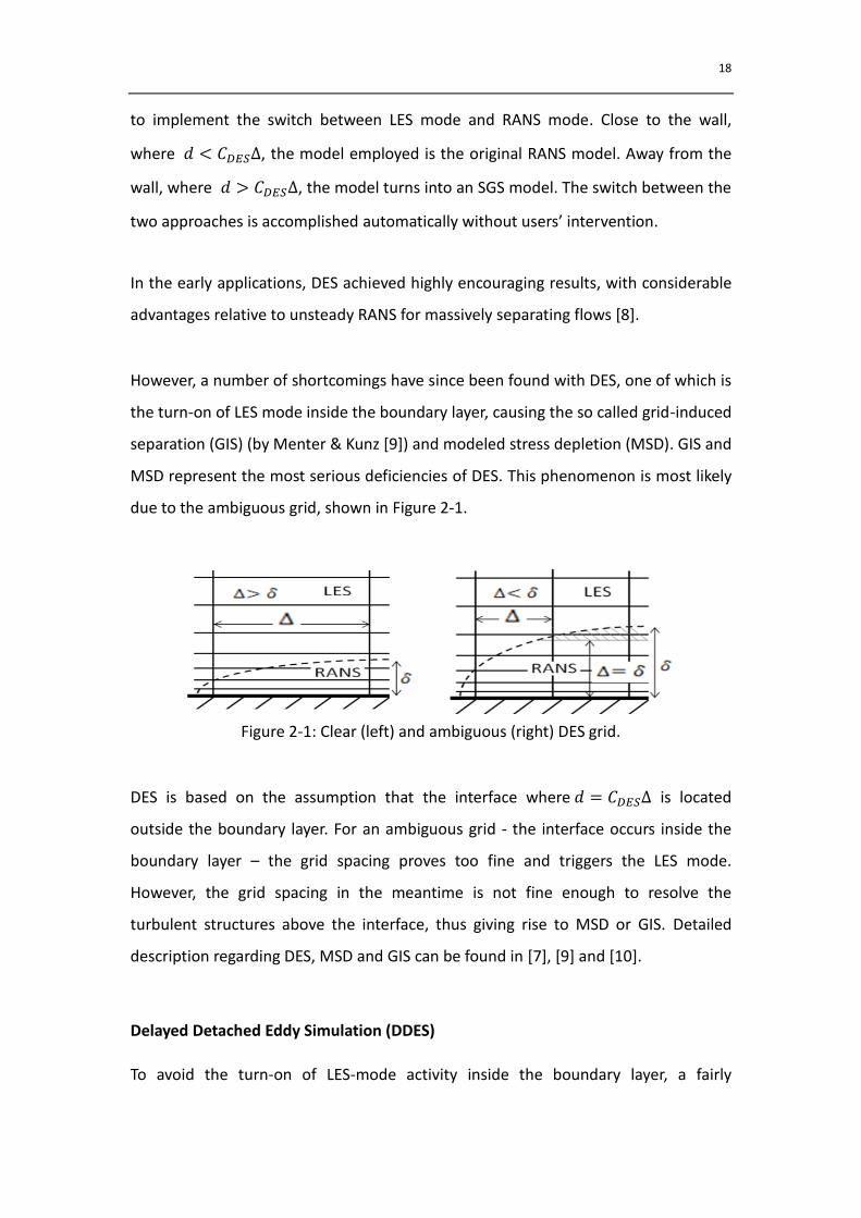
due to the ambiguous grid, shown in Figure 2-1.
Figure 2-1: Clear (left) and ambiguous (right) DES grid.
DES is based on the assumption that the interface where = 𝐶𝐷𝐸 is located
outside the boundary layer. For an ambiguous grid - the interface occurs inside the
boundary layer – the grid spacing proves too fine and triggers the LES mode.
However, the grid spacing in the meantime is not fine enough to resolve the
turbulent structures above the interface, thus giving rise to MSD or GIS. Detailed
description regarding DES, MSD and GIS can be found in [7], [9] and [10].
Delayed Detached Eddy Simulation (DDES)
To avoid the turn-on of LES-mode activity inside the boundary layer, a fairly
19
significant modification of the original DES was made. Instead of depending only on
the grid, solution dependence must be incorporated into the DES length scale
definition. Only with a suitable sensor for the presence of a turbulent boundary layer
can it be ensured that this is modeled by pure RANS.
Spalart et al. (2006) [11] added a shield function f𝑑
to the definition of the
dissipation length scale in Eqn.(2-28).
= − f𝑑𝑚 𝑥{0; − 𝐶𝐷𝐸 } (2-27)
The shield function depends on the boundary layer sensor 𝑟𝑑,
f𝑑
= 1 − tanh[(8𝑟𝑑)3] (2-28)
and 𝑟𝑑 is defined by
𝑟𝑑 =𝜈𝑇 𝜈
𝜅2𝑑2√2 𝑖𝑗 𝑖𝑗
(2-29)
This function assumes the value f𝑑 = 0 inside a turbulent boundary layer, blending
smoothly to f𝑑 = 1 at the boundary layer edge. The shield function delays the
switch to the LES mode until outside the boundary layer. This modification is thus
named Delayed Detached Eddy Simulation.
Scale Adaptive Simulation (SAS)
The Scale Adaptive Simulation (SAS) is an improved unsteady RANS model, with the
ability to adjust to resolved turbulent structures by introducing a second length scale
into the source terms of the underlying turbulence model. Standard two-equation
RANS models like − or − define a turbulent length scale based on the
rate-of-strain (first derivative of velocity) of the mean flow obtained from the
momentum equation, which always return the shear layer thickness as the
appropriate length scale. This leads to an over-predicted length scale and
over-predicted eddy viscosity for flows with resolved structures. In addition to this
length scale, SAS formulations incorporate a second length scale in the form of
20
higher velocity derivatives (typically second derivatives) to provide a reduced eddy
viscosity small enough to allow a break-up of large scales into smaller ones. SAS is
able to provide standard RANS performance in stable flow regions and gives LES-like
behavior in unstable flow regimes [12].
The starting point of SAS is the Rotta’s 𝐿 model, which involves a third derivative
of velocity in the definition of the second length scale. Since a third derivative is
unfavorable to most CFD codes, a reformulation proposed by Menter and Egorov
(1994) yields the 𝐾 𝐾𝐿 (K-Square-root-K-L or − √ 𝐿) model. This model was
further converted into a modification of the widely used − 𝑇 model by
introducing an additional source term in the equation.
SAS is very promising, since it can be simply implemented into an existing RANS
model. However, it is still very young and comparisons of its performance with other
hybrid methods remain to be quantified.

21
2.2 Computational Fluid Dynamics and OpenFOAM
This chapter presents an overview of the subject - computational fluid dynamics (CFD)
and the software used in this research – OpenFOAM. Basic principles and underlying
numerical methods are treated in this chapter. Interested readers are encouraged to
find detailed descriptions in other books and papers (e.g. [13] and [14]).
2.2.1 Overview
Computational fluid dynamics (CFD) is the analysis of systems involving fluid flow,
heat transfer and associated phenomena such as chemical reactions by means of
computer-based simulation [13]. CFD has become a vital component in both research
and industrial application areas. One of the most important advantages of CFD is that
computer-based simulations allow a deeper insight into a system, especially when
the experiment is either unable or too expensive to be executed [13].
A full CFD process consists of three steps: pre-processing, solving and
post-processing [13].
Pre-processing
Pre-processing translates a flow problem into a suitable form and inputs it to a CFD
code. Main procedures include definition of the geometry, generation of mesh,
definition of physical model and definition of boundary conditions.
The geometry of the region of interest – the computational domain, should be
defined in the first place. Then the computational domain is divided into discrete,
smaller and non-overlapping cells by means of mesh generating tools. The definition
of physical model involves the selection of physical and/or chemical phenomena that
need to be modeled and specification of associated fluid and/or chemical properties.
Definition of boundary conditions is to specify the fluid behavior and properties at
22
the cells which coincide with the domain boundary. For transient problems, the
initial conditions also need to be defined. In principle, there are two kinds of
boundary conditions: the Dirichlet boundary condition and the Neumann boundary
condition. The Dirichlet boundary condition specifies a fixed value of a quantity at
the boundary, whereas the Neumann boundary condition prescribes a fixed gradient.
More complicated boundary conditions can be implemented by specifying the
combination of the value and the gradient on the boundary.
Solving
The finite volume (FV) method, which is the most commonly used approach in
well-established CFD code, will be discussed and used in this thesis. The finite
volume approach consists of three steps: integration over each cell, discretization of
the integral equations, and solution of the algebraic equations.
The first step is to integrate the governing equations over each control volume. The
resulting integral equations represent the conservation of relevant properties (e.g.
mass, momentum etc.) for each control volume. In the second step, the integral
equations are converted into a system of algebraic equations through spatial and
temporal discretization. As the volume integral of the convection and diffusion terms
is transformed into the surface integral based on the Gaussian integration, the face
values of cells are introduced into the algebraic equations. A number of discretization
schemes are available in this process. These schemes differ in accuracy, damping and
boundedness of the solution. Finally, the resulting algebraic equations need to be
solved, usually by an iterative approach.
Post-processing
The post-processing step helps users to analyze and visualize the resulting solution.
23
2.2.2 OpenFOAM
A number of commercial CFD packages are able to perform hybrid RANS-LES
simulation and prove to be reliable, such as ANSYS Fluent, ANSYS CFX, Star-CCM+, etc.
In spite of this, this research is carried out with OpenFOAM1.
OpenFOAM, is a free, open source, and object-oriented C++ tool box (including
solvers and utilities) developed for the solution of continuum mechanics, especially
for computational fluid dynamics. OpenFOAM is further supplied with pre- and
post-processing utilities (e.g. ParaView), which enables the users to perform a
complete simulation with a consistent software package. Compared with other CFD
packages, OpenFOAM has its own advantages. Firstly, OpenFOAM is license-free,
which means that it can not only save the users’ acquisition cost, but also enable the
users to do the free-license parallel computing without adding any cost. Secondly,
OpenFOAM enables users to modify existing implementations and even create new
solvers and utilities of their own.
OpenFOAM has also been proved to reliable in hybrid RANS-LES applications carried
out by researchers and industrial users. However, OpenFOAM is still relatively young
and programming errors or inappropriate implementations might exist. Therefore
more verification and validation are needed.
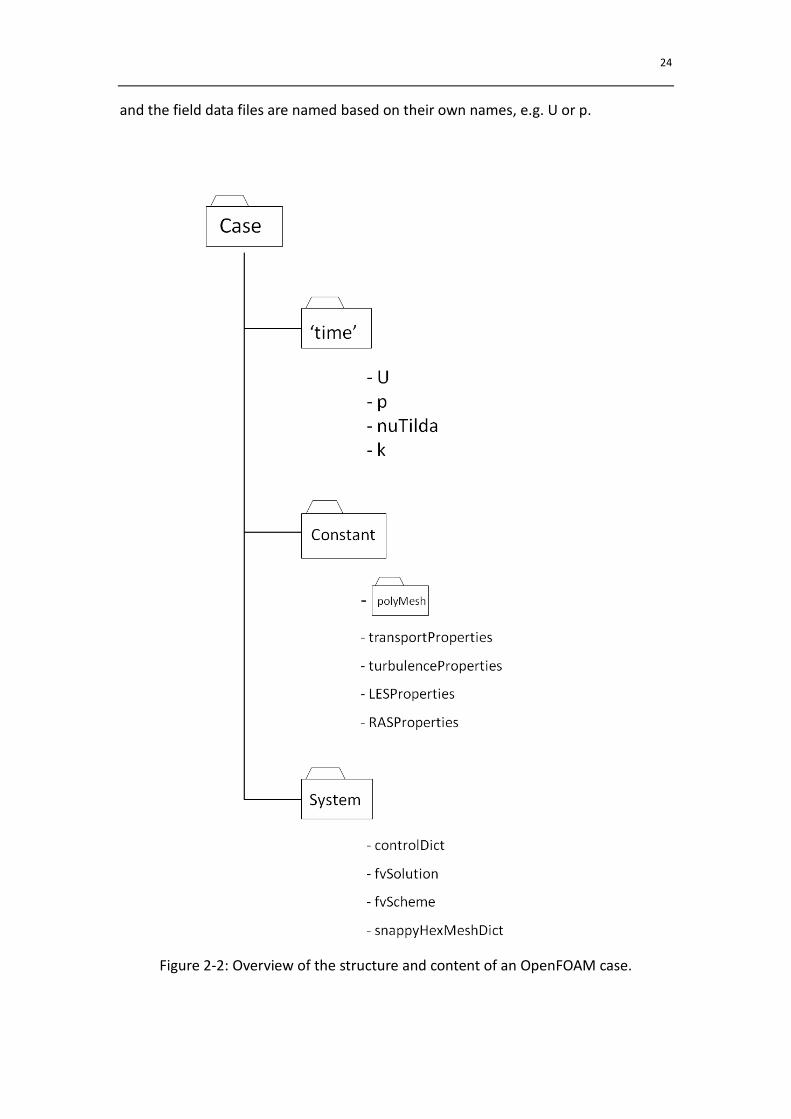
Figure 2-2 gives an overview of the structure of OpenFOAM. A typical OpenFOAM
case consists of three directories: constant, system and ‘time’. The constant directory
contains a number of dictionaries specifying turbulence model and fluid properties,
and a sub-directory – polyMesh containing the mesh information. The dictionaries in
the system directory define the numerical schemes, solution methods and run-time
control parameters. The time directory contains the field data files with boundary
conditions. The name of the directory refers to the physical time of the simulation
1 The version of OpenFOAM used in this work is OpenFOAM-2.1-engysEdition-1.0.
24
and the field data files are named based on their own names, e.g. U or p.
Figure 2-2: Overview of the structure and content of an OpenFOAM case.
25
2.2.3 Finite Volume Discretization
The discretization schemes used in this research are briefly described in this section.
Detailed description and error analyses can be found in [14].
Domain Discretization
OpenFOAM employs the finite volume method to execute CFD simulations. As
described in Section 2.2.1, for the finite volume method, the computational domain
is discretized into a finite number of control volumes (CV) or cells. The control
volumes do not overlap and completely fill the computational domain.
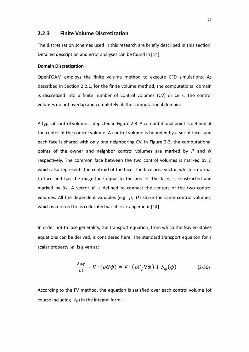
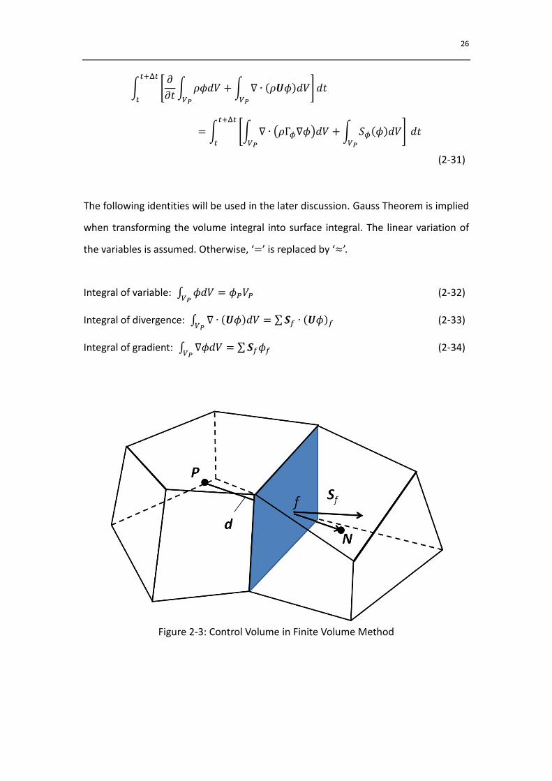
A typical control volume is depicted in Figure 2-3. A computational point is defined at
the center of the control volume. A control volume is bounded by a set of faces and
each face is shared with only one neighboring CV. In Figure 2-3, the computational
points of the owner and neighbor control volumes are marked by and
respectively. The common face between the two control volumes is marked by f,
which also represents the centroid of the face. The face area vector, which is normal
to face and has the magnitude equal to the area of the face, is constructed and
marked by . A vector is defined to connect the centers of the two control
volumes. All the dependent variables (e.g. , ) share the same control volumes,
which is referred to as collocated variable arrangement [14].
In order not to lose generality, the transport equation, from which the Navier-Stokes
equations can be derived, is considered here. The standard transport equaiton for a
scalar property is given as:
𝜕𝜌𝜙
𝜕 + ( ) = ( Γ𝜙 ) + 𝜙( ) (2-30)
According to the FV method, the equation is satisfied over each control volume (of
course including ) in the integral form:
26
∫ [𝜕
𝜕 ∫ 𝑉𝑃
+ ∫ ( ) 𝑉𝑃
] Δ
= ∫ [∫ ( Γ𝜙 ) 𝑉𝑃
+ ∫ 𝜙( ) 𝑉𝑃
] Δ
(2-31)
The following identities will be used in the later discussion. Gauss Theorem is implied
when transforming the volume integral into surface integral. The linear variation of
the variables is assumed. Otherwise, ‘=’ is replaced by ‘≈’.
Integral of variable: ∫ 𝑉𝑃
= (2-32)
Integral of divergence: ∫ ( ) 𝑉𝑃
= ∑ ( ) (2-33)
Integral of gradient: ∫ 𝑉𝑃
= ∑ (2-34)
Figure 2-3: Control Volume in Finite Volume Method
27
Convection Term
After applying Eqs. (2-32) - (2-34), the discretization of the convection term becomes
∫ ( ) 𝑉𝑃
= ∑ ( ) = ∑ ( ) = ∑ (2-35)
where represents the mass flux through the face.
Eqn. (2-35) requires the face values of the variable , which needs to be calculated
from the values of the cell centers. The role of convection differencing schemes is to
determine the face value from the cell center values. For simplicity, only the nearest
neighboring control volumes are used, which is often the case in unstructured
meshes [14]. Therefore to choose convection differencing scheme is in essence to
choose interpolation scheme.
Linear
Assuming linear variation of , the linear interpolation scheme determines the face
value according to [14]
= 𝑥 + (1 − 𝑥) (2-36)
where 𝑥 is the factor defined as the ratio of the distances | | and | |.
𝑥 =| |
| |
The linear interpolation scheme is often referred to as Central Differencing (CD),
which has second order accuracy but boundedness is not guaranteed.
Upwind
The upwind interpolation scheme (Upwind Differencing or UD) determines the face
value of phi according to the direction of the flow. The face value is set equal to the
cell-centered value in the upstream cell. UD guarantees boundedness of the solution
28
but has only first order accuracy [14].
= { 𝑖 𝑚 𝑠𝑠 𝑥 𝑖𝑠 𝑜 𝑜 𝑐 𝑖𝑛 𝑜 𝑖 𝑚 𝑠𝑠 𝑥 𝑖𝑠 𝑜 𝑜 𝑐 𝑖𝑛 𝑜
(2-37)
Linear-upwind
The linear-upwind interpolation scheme (Liner Upwind Differencing or LUD) attempts
to preserve both boundedness and second order accuracy. The face value is
computed by the following expression:
= + (2-38)
where and are the cell-centered values and its gradient in the upstream cell,
and is the displacement vector from the upstream cell centroid to the face
centroid. Specifically, the face value is given by:
= { + ( ) 𝑖 𝑚 𝑠𝑠 𝑥 𝑖𝑠 𝑜 𝑜 𝑐 𝑖𝑛 𝑜
+ ( ) 𝑖 𝑚 𝑠𝑠 𝑥 𝑖𝑠 𝑜 𝑜 𝑐 𝑖𝑛 𝑜 (2-39)
This formulation requires extra specification of gradient schemes.
LUST
The linear-upwind stabilized transport (LUST) is an interpolation scheme in which
linear-upwind is blended with linear interpolation to stabilize solutions while
maintaining second-order behavior. A blending factor γ is used to optimize the
balance between accuracy and stability in Eqn. (2-40). For standard LUST in
OpenFOAM, the blending factor is set to 0.75 linear, whereas the factor is set to 0.90
for the modified scheme - LUST10. LUST has been reported to prove particularly
successful for LES/DES in complex geometries with complex unstructured meshes.
= 𝛾( )𝐶𝐷+ (1 − 𝛾)( )𝐿 𝐷
(2-40)

29
Diffusion Term
Similar to the convection term, applying Eqs. (2-32) - (2-34), the discretization of the
diffusion term becomes
∫ ( Γ𝜙 ) 𝑉𝑃
= ∑ ( Γ𝜙 ) = ∑ ( Γ𝜙)
( ) (2-41)
The right hand side of Eqn. (2-41) needs to be evaluated with appropriate
methodologies. The face value of the scalar Γ𝜙 can be interpolated from
cell-centered values. When the transported variable is the velocity in an
incompressible flow, the transport equation reduces to Eqn. (2-41) and Γ𝜙
becomes a constant i.e. Γ𝜙 = . The dot product part ( ) which is mesh
dependent requires special care and is discussed below.
If the mesh is orthogonal, i.e. distance vector and face area vector are in
parallel, the dot product is expressed by [14]
( ) = | | 𝜙𝑁−𝜙𝑃
| | (2-42)
The mesh is however non-orthogonal in many cases. Therefore an additional term is
used to correct the formula. The face area vector is decomposed into two parts
and correspondingly the dot product is a summation of two parts: the orthogonal
part and the non-orthogonal correction part.
= +
(2-43)
( ) = ( ) ⏟
𝑜 ℎ𝑜𝑔𝑜𝑛𝑎
+ ( ) ⏟
𝑛𝑜𝑛−𝑜 ℎ𝑜𝑔𝑜𝑛𝑎
(2-44)
The vector is decomposed into vector and vector
in Eqn. (2-43),
is chosen to be parallel with , which allows the use of Eqn. (2-42) on the
30
orthogonal part.
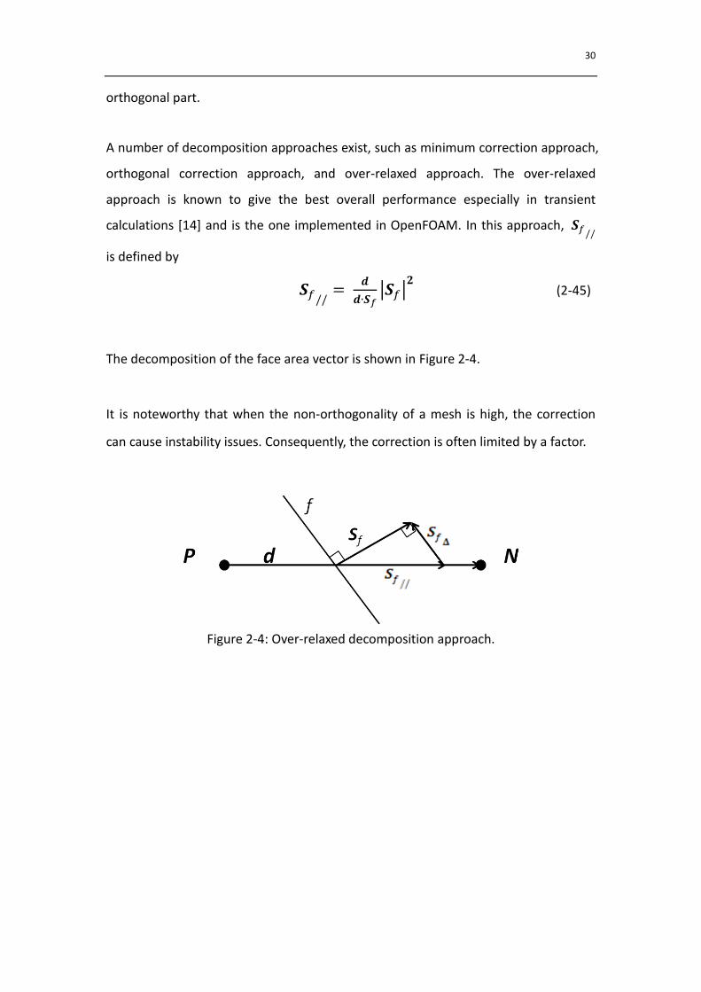
A number of decomposition approaches exist, such as minimum correction approach,
orthogonal correction approach, and over-relaxed approach. The over-relaxed
approach is known to give the best overall performance especially in transient
calculations [14] and is the one implemented in OpenFOAM. In this approach,
is defined by
=
𝑓| |
𝟐 (2-45)
The decomposition of the face area vector is shown in Figure 2-4.
It is noteworthy that when the non-orthogonality of a mesh is high, the correction
can cause instability issues. Consequently, the correction is often limited by a factor.
Figure 2-4: Over-relaxed decomposition approach.
31
Temporal Discretization
In the previous section, the discretization of spatial term has been presented. This
can be split into two parts – the transformation of surface and volume integral into
discrete summations and expressions that give the face values of the variables as a
function of cell-centered values. Assuming the control volume does not change in
time, applying the spatial discretization to Eqn. (2-30) yields a semi-discrete
equation:
∫ [(𝜕𝜌𝜙
𝜕 ) ]
Δ
= ∫ ℱ( )
Δ
(2-46)
where ℱ( ) represents a function of cell-centered values of .
Depending on how to discretize the left hand side and right hand side of the
equation, a number of schemes have been proposed. As this research assumes
incompressible flow, which means the density is a constant everywhere and every
time, both the left hand side and right hand side are divided by , resulting in a
temporal derivative only with respect to .
Explicit
In the explicit discretization, the right hand side of Eqn. (2-46) depends only on the
old-time field.
𝜙𝑛−𝜙𝑛−1
= ℱ( 𝑛−1) (2-47)
where
𝑛 = ( + )
𝑛−1 = ( )
and hereinafter.
32
This method is simple and straightforward but has only first order accuracy. The
value of at new time level is calculated directly without solving a matrix equation.
The major drawback of this method, however, is the stability issue when the Courant
number limit is violated. The Courant number is defined as:
𝐶 𝐿 =
| |2 (2-48)
where is the distance vector between the adjacent cell centers and is the
velocity vector at the cell face. To avoid instability, the Courant number should be
kept below unity when using the explicit method.
Euler Implicit
The Euler Implicit method (named Euler in OpenFOAM) expresses the right hand side
using the face values and center value of the new time level, yielding:
𝜙𝑛−𝜙𝑛−1
= ℱ( 𝑛) (2-49)
Euler is still first order accurate, but unlike the explicit method, a system of algebraic
equations regarding the new value has to be solved. The system is strongly coupled
and can be stable even if the Courant number limit is not strictly satisfied.
Crank – Nicholson
The Crank – Nicholson method expresses the right hand side using the arithmetic
average of the values at both the new time level and old time level.
𝜙𝑛−𝜙𝑛−1
=
1
2(ℱ( 𝑛) + ℱ( 𝑛−1)) (2-50)
The Crank – Nicholson method of temporal discretization is second order accurate
33
and similar to Euler, a system of algebraic equations needs to be solved to determine
the new time-level value. The Crank–Nicolson scheme is unconditionally stable. The
solutions can however still suffer from spurious oscillations. For this reason,
whenever large time steps or high spatial resolution is necessary, the less accurate
backward method is often used, which is both stable and immune to oscillations.
Backward
The second order Backward (named Backward in OpenFOAM) differencing is an
implicit temporal scheme with second order accuracy, which employs values at three
time steps to approximate the time derivative at the left hand side. The time
derivative is replaced by a second order approximation and new time-level values are
used in the right hand side, which gives:
3
2
𝑛𝜙𝑛−2𝜙𝑛−1
1
2𝜙𝑛−2
= ℱ( 𝑛) (2-51)
where 𝑛−2 = ( − ).
34
2.2.4 Solution
Eqn. (2-5) and Eqn. (2-6) are the governing equations for a time-dependent
incompressible Newtonian fluid flow, rewritten below. These two equations are
treated in this subsection as an example, since the filtered or Reynolds averaged
equations share similar forms and similar treatment procedures.
= 0
(2-5) 𝜕
𝜕 + ( ) = − +
( ) (2-6)
There are two main difficulties to solve these equations:
1) The convection term is non-linear, since velocity is ‘being transported by itself’.
2) Velocity and pressure are coupled in these equations.
Therefore the solution of these equations requires two procedures: linearization of
the momentum equations Eqn. (2-6); and implementation of a pressure-velocity
coupling algorithm. These procedures will be presented in the following subsections.
Linearization
Eqn. (2-52) gives the discretization of the convection term
( ) = ∑ = ∑ (2-52)
where is the face flux, is the face value of velocity interpolated from the
cell-centered values. The challenge is that the face fluxes are a function of .
Linearization of the convection term means that the fluxes will be calculated from an
existing velocity field that satisfies the continuity equation. The fact that the fluxes
are calculated from existing velocities implies that the information is lagged. In order
35
to capture the non-linearity and reduce the error caused by the lagged information,
either sub-iteration over the entire algorithm so that the lagged velocities and thus
the fluxes are iteratively updated; or use of small time step so that the error induced
by the lagged information remains small, must be adopted [14].
Pressure-Velocity Coupling
As the continuity equation does not contain the time dependent term, the velocities
at the new time level are derived from the momentum equations and the continuity
equation serves as a constraint of the velocity field. Because of the pressure-velocity
coupling, solution of the momentum equation demands an existing pressure field. An
initial guess or the pressure from last time level is usually used as an estimate. If the
estimate is not true, however, the velocity solution from the momentum equation
does not satisfy the continuity equation. To solve this problem, a pressure equation
needs to be derived.
A general form of the semi-discrete momentum equations for a control volume
can be written as:
+ ∑ = 𝑹𝑪 − (2-53)
where and are the diagonal and off-diagonal coefficients respectively, and
𝑹𝑪 is the source vector which includes the part of the transient term and all other
source terms except the pressure gradient. The pressure gradient is left out of
the source vector to enable the derivation of the pressure equation.
Introduce a new operator ( ):
( ) = −∑ + 𝑹𝑪 (2-54)
The ( ) term consists of two parts, the ”transport part” including the coefficients
36
for all neighbors multiplied by corresponding velocities −∑ 𝑈 , and the
“source-term part” including the source part of the transient term and all other
source terms (except the pressure gradient) 𝑹𝑪 . For instance, ( ) for the
incompressible Navier-Stokes equations (excluding all other additional terms) using
Euler implicit temporal differencing is:
( ) = −∑ + 0
(2-55)
Note that the operator ( ) is a function of both the present velocity and the
velocity of the previous time level (and 𝟎𝟎 if Backward temporal differencing
is used) and in the next section ( ) is written in the form of ( 𝟎) to make it
clear. In addition, the coefficient in the operator depends on the face fluxes
which need to be constructed from the velocity field. This non-linearity raises the
difficulty in solving the system.
Move the off-diagonal terms to the right hand side and Eqn. (2-56) is obtained:
= ( ) − (2-56)
Eqn. (2-56) can be solved for the velocity at the cell center by dividing by , yielding
= ( )
𝑎𝑃−
1
𝑎𝑃 (2-57)
The velocity at the cell faces can be obtained through interpolation from cell centers,
i.e.
= ( ( )
𝑎𝑃) − (
1
𝑎𝑃) ( ) (2-58)
This equation will also be used later to calculate the face fluxes. The discretized
continuity equation is written as
37
= ∑ = 0 (2-59)
Substitution of Eqn. (2-58) into Eqn. (2-59) gives the discretized pressure equation:
(1
𝑎𝑃 ) = ∑ [(
1
𝑎𝑃) ( ) ] = ∑ (
( )
𝑎𝑃)
(2-60)
The final form of the discretized incompressible Navier–Stokes equations is written
as below:
momentum prediction:
= ( ) − (2-61)
pressure equation:
∑ [(1
𝑎𝑃) ( ) ] = ∑ (
( )
𝑎𝑃)
(2-62)
Finally, the face fluxes are computed using from Eqn. (2-63).
= = [( ( )
𝑎𝑃) − (
1
𝑎𝑃) ( ) ] (2-63)
Apparently the face fluxes are guaranteed to be conservative.
The discretized form of the Navier–Stokes system in Eqn. (2-61) and Eqn. (2-62) are
coupled in velocity and pressure. Due to the high computational efforts of the
existing simultaneous algorithms which solve the full-coupled system of equations
simultaneously, the commonly used methods are the segregated methods such as
PISO and SIMPLE. In OpenFOAM, PISO and SIMPLE are typically used for transient
and steady problems respectively. Instead of PISO, a SIMPLE based in-house transient
solver named transientSimpleFoam is used in this research. Transient SIMPLE
approaches are known to be robust and allow a relatively larger time step [13]. A
brief description of this solver is given in this subsection.
38
The main procedure of transientSimpleFoam is given as follows:
𝑛: Time step index
𝑖: SIMPLE inner loop index
1) Increment time: 𝑛 = 𝑛−1 +
2) Start SIMPLE inner loop: 𝑛 = 𝑛−1 𝑛 = 𝑛−1 𝑛 = 𝑛−1
a) Assemble and solve the momentum predictor equation Eqn. (2-64) for
predicted velocity 𝑛 with the available face fluxes and pressure field. Note
that the equation is under-relaxed in an implicit manner with the velocity
under-relaxation factor (0 < < 1).
𝑎𝑃
𝛼𝑈
𝑛 = 𝑛 −1( 𝑛 𝑛−1) − ∑ ( 𝑛 −1)
+
1−𝛼𝑈
𝛼𝑈
𝑛−1 (2-64)
b) Formulate and solve the pressure equation Eqn. (2-65) to obtain the new
pressure field 𝑛 .
∑ [(1
𝑎𝑃) ( 𝑛 )
] = ∑ (
𝑛𝑖−1( 𝑛 𝑖 𝑛−1)
𝑎𝑃)
(2-65)
c) Calculate a new set of conservative face fluxes satisfying the continuity
equation using Eqn. (2-66). The operator is reconstructed using the new
set of conservative face fluxes - 𝑛 .
= = [( 𝑛
𝑖 ( 𝑛 𝑖 𝑛−1)
𝑎𝑃) − (
1
𝑎𝑃) ( 𝑛 )
] (2-66)
d) Correct the pressure solution by the pressure under-relaxation factor
(0 < < 1).
𝑛 = 𝑛 −1 + ( 𝑛 − 𝑛 −1) (2-67)
39
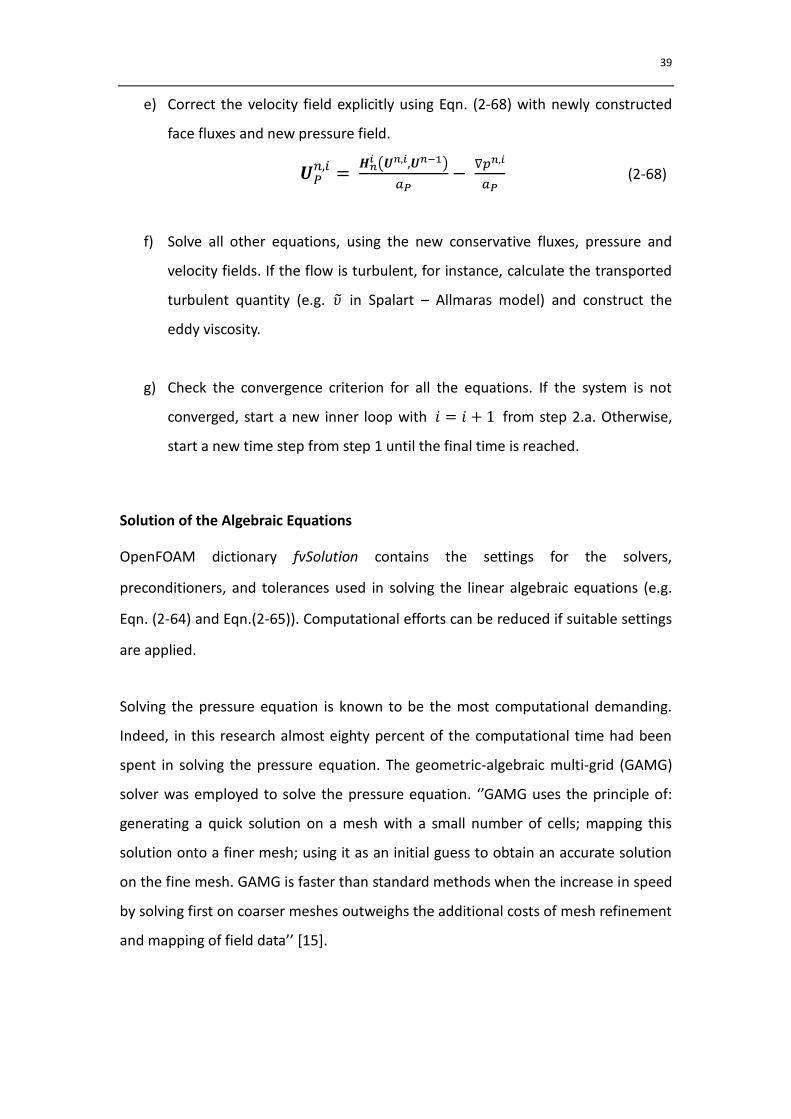
e) Correct the velocity field explicitly using Eqn. (2-68) with newly constructed
face fluxes and new pressure field.
𝑛 =
𝑛𝑖 ( 𝑛 𝑖 𝑛−1)
𝑎𝑃−
𝑛 𝑖
𝑎𝑃 (2-68)
f) Solve all other equations, using the new conservative fluxes, pressure and
velocity fields. If the flow is turbulent, for instance, calculate the transported
turbulent quantity (e.g. �� in Spalart – Allmaras model) and construct the
eddy viscosity.
g) Check the convergence criterion for all the equations. If the system is not
converged, start a new inner loop with 𝑖 = 𝑖 + 1 from step 2.a. Otherwise,
start a new time step from step 1 until the final time is reached.
Solution of the Algebraic Equations
OpenFOAM dictionary fvSolution contains the settings for the solvers,
preconditioners, and tolerances used in solving the linear algebraic equations (e.g.
Eqn. (2-64) and Eqn.(2-65)). Computational efforts can be reduced if suitable settings
are applied.
Solving the pressure equation is known to be the most computational demanding.
Indeed, in this research almost eighty percent of the computational time had been
spent in solving the pressure equation. The geometric-algebraic multi-grid (GAMG)
solver was employed to solve the pressure equation. ‘’GAMG uses the principle of:
generating a quick solution on a mesh with a small number of cells; mapping this
solution onto a finer mesh; using it as an initial guess to obtain an accurate solution
on the fine mesh. GAMG is faster than standard methods when the increase in speed
by solving first on coarser meshes outweighs the additional costs of mesh refinement
and mapping of field data’’ [15].
40
3. Cases and Results
In this chapter, the numerical simulation cases are described in detail and associated
results are presented. Section 3.1 gives an overview of the related numerical and
experimental studies of the test case. The detailed settings for numerical simulation
are given in Section 3.2. The results are analyzed and compared to the experimental
measurements in both unsteady flow phenomena and time averaged flow field in
Section 3.3.
3.1 Test Case Description
Similar studies regarding aero-acoustic process in simplified HVAC ducts have been
carried out by other researchers both numerically and experimentally. Therefore the
test case selected in this research is the same as in the published studies so as to
make comparisons with other researchers’ results.
3.1.1 Geometry – Simplified HVAC duct
The test case is chosen to have a quite simple geometry in order that the meshing
effort to generate the grids could be kept small and that the amount of cells could be
kept in a reasonable range to keep the computation time affordable. Despite the
simple geometry, the test case shows a rather complex three-dimensional flow,
which can serve as a representative for flows occurring in real life HVAC components.
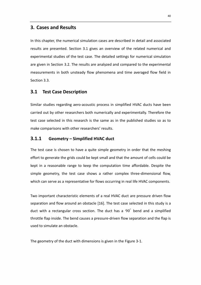
Two important characteristic elements of a real HVAC duct are pressure driven flow
separation and flow around an obstacle [16]. The test case selected in this study is a
duct with a rectangular cross section. The duct has a 90° bend and a simplified
throttle flap inside. The bend causes a pressure-driven flow separation and the flap is
used to simulate an obstacle.
The geometry of the duct with dimensions is given in the Figure 3-1.
41
Figure 3-1: Geometry of the simplified HVAC duct
3.1.2 Experimental Rig
The selected test case had been investigated experimentally by the consortium of
German car manufactures Audi, BMW, Daimler, Porsche and Volkswagen and the
results had been presented by the consortium in Jäger et al (2008) [16]. The
experimental setup is briefly described in this section. More details can be found in
Jäger et al (2008) [16].
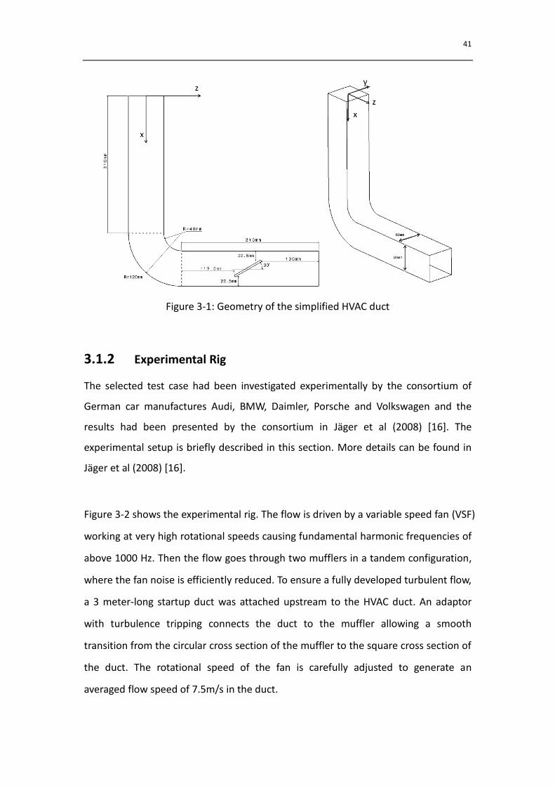
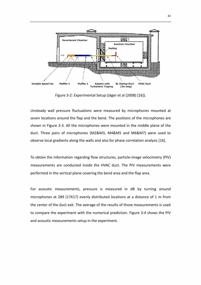
Figure 3-2 shows the experimental rig. The flow is driven by a variable speed fan (VSF)
working at very high rotational speeds causing fundamental harmonic frequencies of
above 1000 Hz. Then the flow goes through two mufflers in a tandem configuration,
where the fan noise is efficiently reduced. To ensure a fully developed turbulent flow,
a 3 meter-long startup duct was attached upstream to the HVAC duct. An adaptor
with turbulence tripping connects the duct to the muffler allowing a smooth
transition from the circular cross section of the muffler to the square cross section of
the duct. The rotational speed of the fan is carefully adjusted to generate an
averaged flow speed of 7.5m/s in the duct.
42
Figure 3-2: Experimental Setup (Jäger et al (2008) [16]).
Unsteady wall pressure fluctuations were measured by microphones mounted at
seven locations around the flap and the bend. The positions of the microphones are
shown in Figure 3-3. All the microphones were mounted in the middle plane of the
duct. Three pairs of microphones (M2&M3, M4&M5 and M6&M7) were used to
observe local gradients along the walls and also for phase correlation analysis [16].
To obtain the information regarding flow structures, particle-image velocimetry (PIV)
measurements are conducted inside the HVAC duct. The PIV measurements were
performed in the vertical plane covering the bend area and the flap area.
For acoustic measurements, pressure is measured in dB by turning around
microphones at 289 (17X17) evenly distributed locations at a distance of 1 m from
the center of the duct exit. The average of the results of those measurements is used
to compare the experiment with the numerical prediction. Figure 3-4 shows the PIV
and acoustic measurements setup in the experiment.
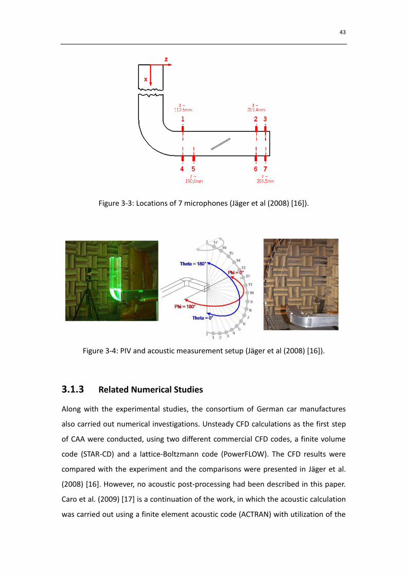
43
Figure 3-3: Locations of 7 microphones (Jäger et al (2008) [16]).
Figure 3-4: PIV and acoustic measurement setup (Jäger et al (2008) [16]).
3.1.3 Related Numerical Studies
Along with the experimental studies, the consortium of German car manufactures
also carried out numerical investigations. Unsteady CFD calculations as the first step
of CAA were conducted, using two different commercial CFD codes, a finite volume
code (STAR-CD) and a lattice-Boltzmann code (PowerFLOW). The CFD results were
compared with the experiment and the comparisons were presented in Jäger et al.
(2008) [16]. However, no acoustic post-processing had been described in this paper.
Caro et al. (2009) [17] is a continuation of the work, in which the acoustic calculation
was carried out using a finite element acoustic code (ACTRAN) with utilization of the
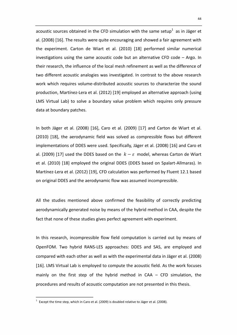
44
acoustic sources obtained in the CFD simulation with the same setup1 as in Jäger et
al. (2008) [16]. The results were quite encouraging and showed a fair agreement with
the experiment. Carton de Wiart et al. (2010) [18] performed similar numerical
investigations using the same acoustic code but an alternative CFD code – Argo. In
their research, the influence of the local mesh refinement as well as the difference of
two different acoustic analogies was investigated. In contrast to the above research
work which requires volume-distributed acoustic sources to characterize the sound
production, Martínez-Lera et al. (2012) [19] employed an alternative approach (using
LMS Virtual Lab) to solve a boundary value problem which requires only pressure
data at boundary patches.
In both Jäger et al. (2008) [16], Caro et al. (2009) [17] and Carton de Wiart et al.
(2010) [18], the aerodynamic field was solved as compressible flows but different
implementations of DDES were used. Specifically, Jäger et al. (2008) [16] and Caro et
al. (2009) [17] used the DDES based on the − model, whereas Carton de Wiart
et al. (2010) [18] employed the original DDES (DDES based on Spalart-Allmaras). In
Martínez-Lera et al. (2012) [19], CFD calculation was performed by Fluent 12.1 based
on original DDES and the aerodynamic flow was assumed incompressible.
All the studies mentioned above confirmed the feasibility of correctly predicting
aerodynamically generated noise by means of the hybrid method in CAA, despite the
fact that none of these studies gives perfect agreement with experiment.
In this research, incompressible flow field computation is carried out by means of
OpenFOM. Two hybrid RANS-LES approaches: DDES and SAS, are employed and
compared with each other as well as with the experimental data in Jäger et al. (2008)
[16]. LMS Virtual Lab is employed to compute the acoustic field. As the work focuses
mainly on the first step of the hybrid method in CAA – CFD simulation, the
procedures and results of acoustic computation are not presented in this thesis.
1 Except the time step, which in Caro et al. (2009) is doubled relative to Jäger et al. (2008).
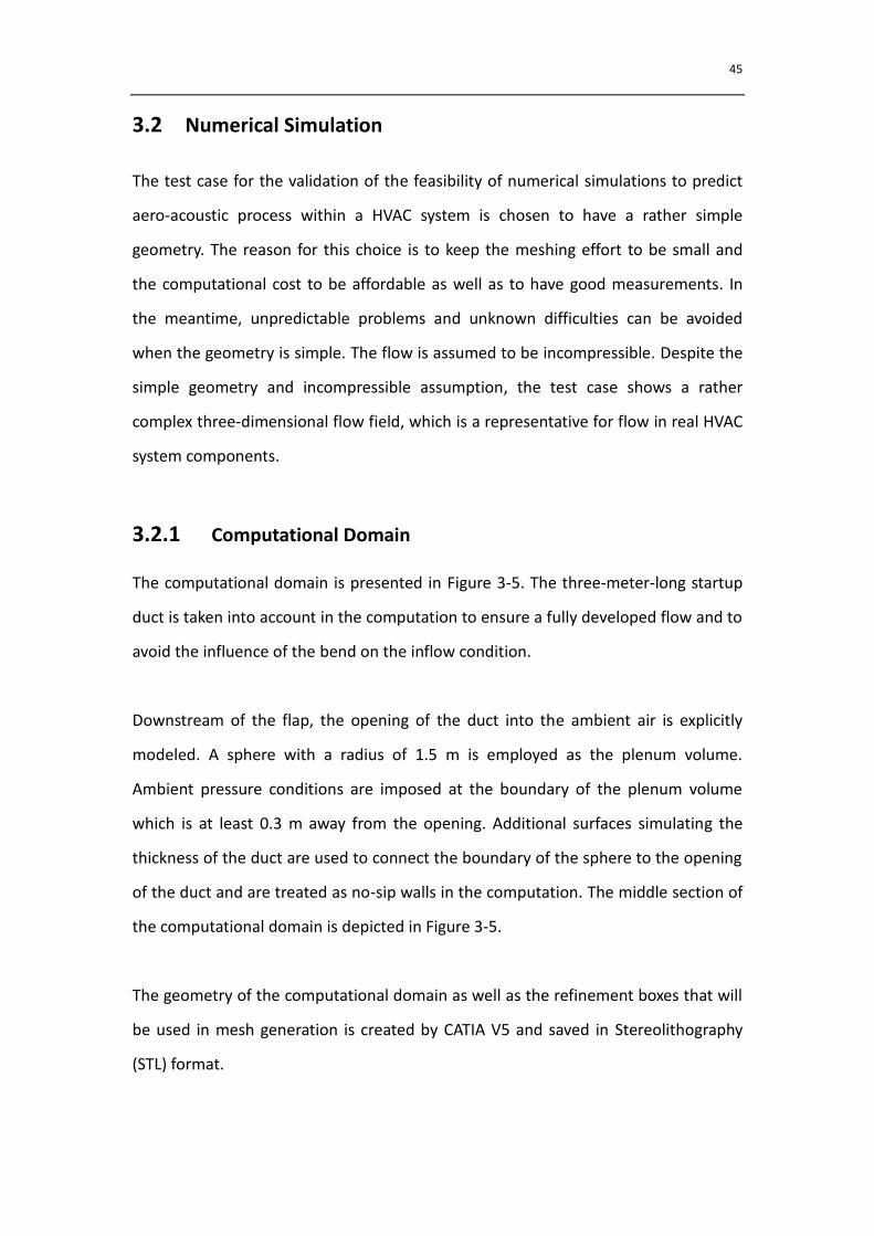
45
3.2 Numerical Simulation
The test case for the validation of the feasibility of numerical simulations to predict
aero-acoustic process within a HVAC system is chosen to have a rather simple
geometry. The reason for this choice is to keep the meshing effort to be small and
the computational cost to be affordable as well as to have good measurements. In
the meantime, unpredictable problems and unknown difficulties can be avoided
when the geometry is simple. The flow is assumed to be incompressible. Despite the
simple geometry and incompressible assumption, the test case shows a rather
complex three-dimensional flow field, which is a representative for flow in real HVAC
system components.
3.2.1 Computational Domain
The computational domain is presented in Figure 3-5. The three-meter-long startup
duct is taken into account in the computation to ensure a fully developed flow and to
avoid the influence of the bend on the inflow condition.
Downstream of the flap, the opening of the duct into the ambient air is explicitly
modeled. A sphere with a radius of 1.5 m is employed as the plenum volume.
Ambient pressure conditions are imposed at the boundary of the plenum volume
which is at least 0.3 m away from the opening. Additional surfaces simulating the
thickness of the duct are used to connect the boundary of the sphere to the opening
of the duct and are treated as no-sip walls in the computation. The middle section of
the computational domain is depicted in Figure 3-5.
The geometry of the computational domain as well as the refinement boxes that will
be used in mesh generation is created by CATIA V5 and saved in Stereolithography
(STL) format.

46
Figure 3-5: Geometry of the computational domain.
3.2.2 Meshing
The meshing tool employed in this research is the snappyHexMesh, the mesh
generation utility supplied with OpenFOAM. The snappyHexMesh utility generates
three-dimensional meshes containing hexahedra and split hexahedra automatically
from triangulated surface geometries in STL format. The specification of mesh
refinement level is very flexible and the surface handling is robust with a
pre-specified final mesh quality. It runs in parallel with a load balancing step every
iteration’’ [15].
The whole process of the mesh generation and the quality of the final mesh are
controlled by the entries in the snappyHexMeshDict dictionary, located in the system
sub-directory of the case.
The simulation has been executed on two different grids. Both the grids have been
done with local refinements around the bend and in the jet. As most of the
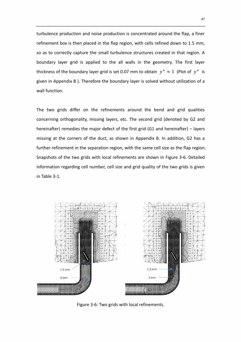
47
turbulence production and noise production is concentrated around the flap, a finer
refinement box is then placed in the flap region, with cells refined down to 1.5 mm,
so as to correctly capture the small turbulence structures created in that region. A
boundary layer grid is applied to the all walls in the geometry. The first layer
thickness of the boundary layer grid is set 0.07 mm to obtain ≈ 1 (Plot of is
given in Appendix B ). Therefore the boundary layer is solved without utilization of a
wall function.
The two grids differ on the refinements around the bend and grid qualities
concerning orthogonality, missing layers, etc. The second grid (denoted by G2 and
hereinafter) remedies the major defect of the first grid (G1 and hereinafter) – layers
missing at the corners of the duct, as shown in Appendix B. In addition, G2 has a
further refinement in the separation region, with the same cell size as the flap region.
Snapshots of the two grids with local refinements are shown in Figure 3-6. Detailed
information regarding cell number, cell size and grid quality of the two grids is given
in Table 3-1.
Figure 3-6: Two grids with local refinements.
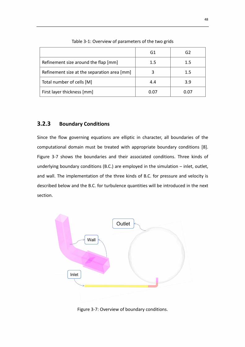
48
Table 3-1: Overview of parameters of the two grids
G1 G2
Refinement size around the flap [mm] 1.5 1.5
Refinement size at the separation area [mm] 3 1.5
Total number of cells [M] 4.4 3.9
First layer thickness [mm] 0.07 0.07
3.2.3 Boundary Conditions
Since the flow governing equations are elliptic in character, all boundaries of the
computational domain must be treated with appropriate boundary conditions [8].
Figure 3-7 shows the boundaries and their associated conditions. Three kinds of
underlying boundary conditions (B.C.) are employed in the simulation – inlet, outlet,
and wall. The implementation of the three kinds of B.C. for pressure and velocity is
described below and the B.C. for turbulence quantities will be introduced in the next
section.
Figure 3-7: Overview of boundary conditions.
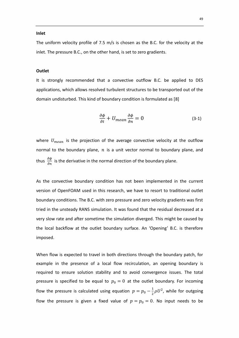
49
Inlet
The uniform velocity profile of 7.5 m/s is chosen as the B.C. for the velocity at the
inlet. The pressure B.C., on the other hand, is set to zero gradients.
Outlet
It is strongly recommended that a convective outflow B.C. be applied to DES
applications, which allows resolved turbulent structures to be transported out of the
domain undisturbed. This kind of boundary condition is formulated as [8]
𝜕𝜙
𝜕 + 𝑈 𝑎𝑛
𝜕𝜙
𝜕𝑛= 0 (3-1)
where 𝑈 𝑎𝑛 is the projection of the average convective velocity at the outflow
normal to the boundary plane, 𝑛 is a unit vector normal to boundary plane, and
thus 𝜕𝜙
𝜕𝑛 is the derivative in the normal direction of the boundary plane.
As the convective boundary condition has not been implemented in the current
version of OpenFOAM used in this research, we have to resort to traditional outlet
boundary conditions. The B.C. with zero pressure and zero velocity gradients was first
tried in the unsteady RANS simulation. It was found that the residual decreased at a
very slow rate and after sometime the simulation diverged. This might be caused by
the local backflow at the outlet boundary surface. An ‘Opening’ B.C. is therefore
imposed.
When flow is expected to travel in both directions through the boundary patch, for
example in the presence of a local flow recirculation, an opening boundary is
required to ensure solution stability and to avoid convergence issues. The total
pressure is specified to be equal to = 0 at the outlet boundary. For incoming
flow the pressure is calculated using equation = −1
2 𝑈2, while for outgoing
flow the pressure is given a fixed value of = = 0. No input needs to be
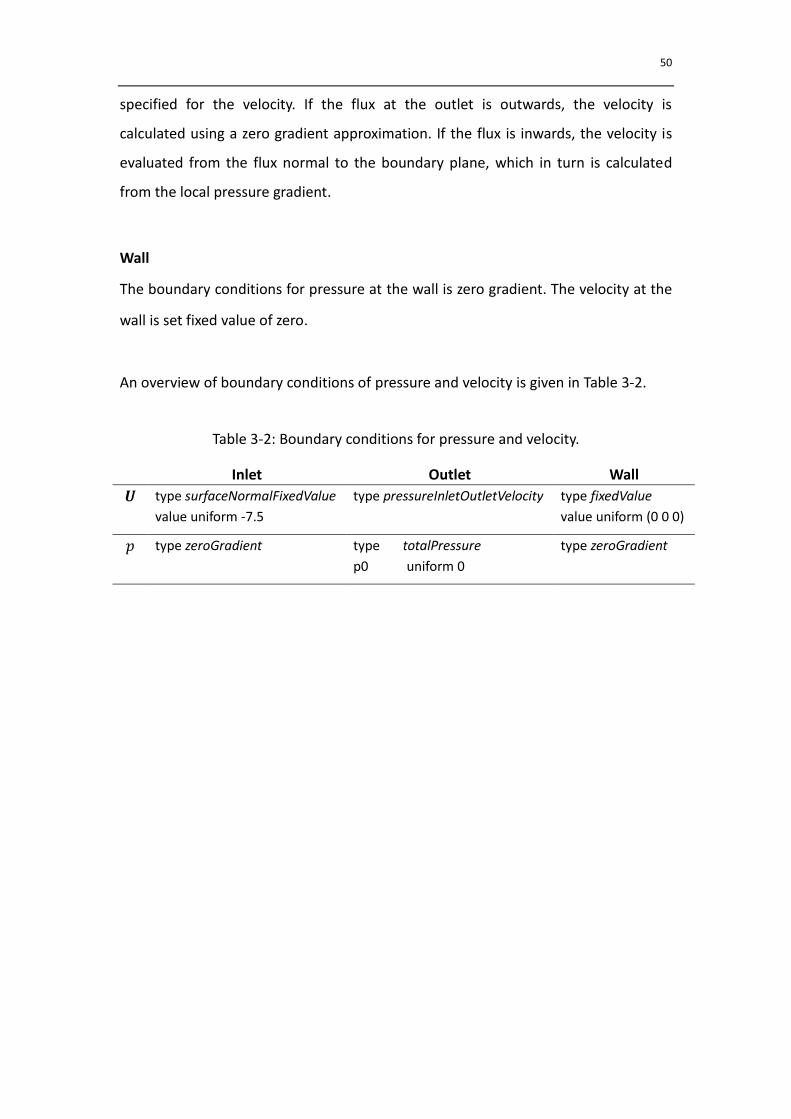
50
specified for the velocity. If the flux at the outlet is outwards, the velocity is
calculated using a zero gradient approximation. If the flux is inwards, the velocity is
evaluated from the flux normal to the boundary plane, which in turn is calculated
from the local pressure gradient.
Wall
The boundary conditions for pressure at the wall is zero gradient. The velocity at the
wall is set fixed value of zero.
An overview of boundary conditions of pressure and velocity is given in Table 3-2.
Table 3-2: Boundary conditions for pressure and velocity.
Inlet Outlet Wall
type surfaceNormalFixedValue
value uniform -7.5
type pressureInletOutletVelocity type fixedValue
value uniform (0 0 0)
type zeroGradient type totalPressure
p0 uniform 0
type zeroGradient
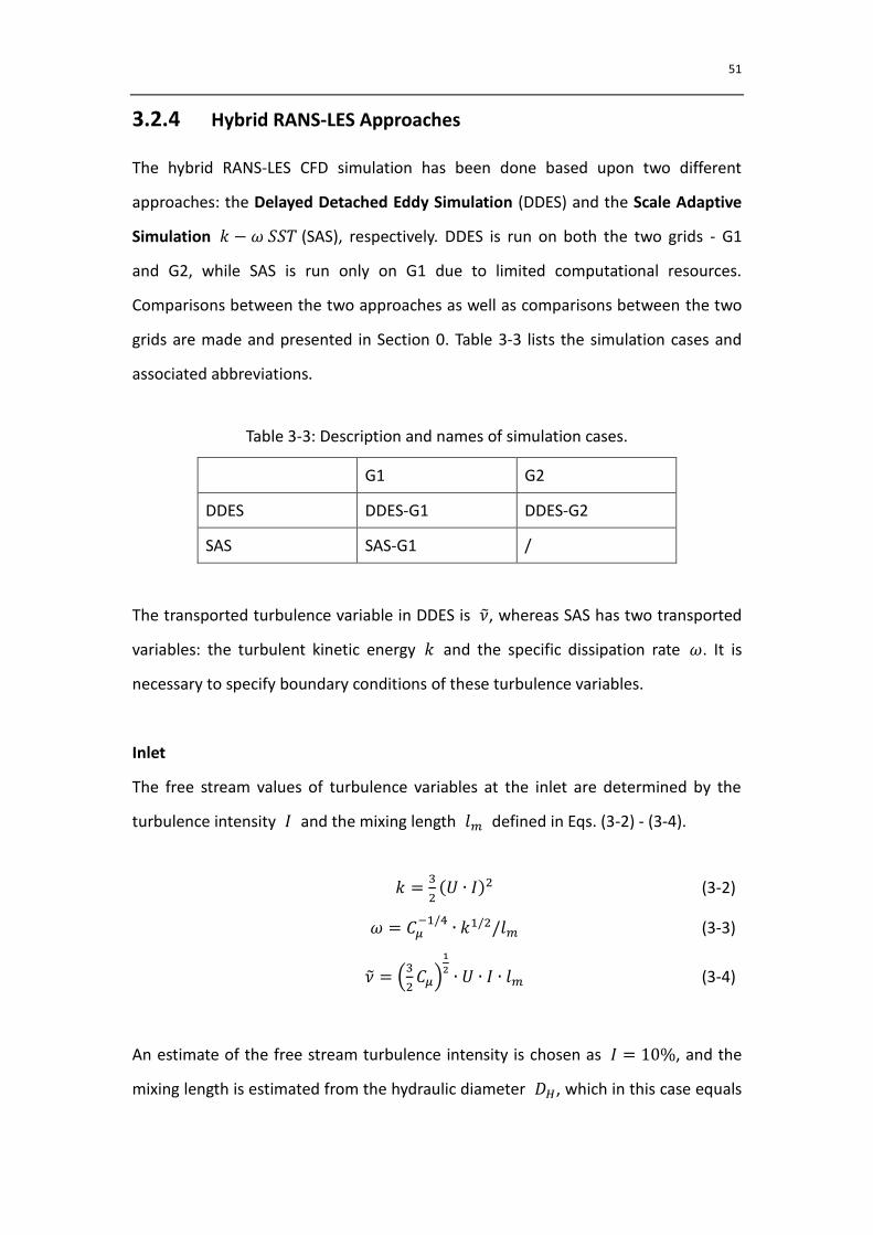
51
3.2.4 Hybrid RANS-LES Approaches
The hybrid RANS-LES CFD simulation has been done based upon two different
approaches: the Delayed Detached Eddy Simulation (DDES) and the Scale Adaptive
Simulation − 𝑇 (SAS), respectively. DDES is run on both the two grids - G1
and G2, while SAS is run only on G1 due to limited computational resources.
Comparisons between the two approaches as well as comparisons between the two
grids are made and presented in Section 0. Table 3-3 lists the simulation cases and
associated abbreviations.
Table 3-3: Description and names of simulation cases.
G1 G2
DDES DDES-G1 DDES-G2
SAS SAS-G1 /
The transported turbulence variable in DDES is , whereas SAS has two transported
variables: the turbulent kinetic energy and the specific dissipation rate . It is
necessary to specify boundary conditions of these turbulence variables.
Inlet
The free stream values of turbulence variables at the inlet are determined by the
turbulence intensity and the mixing length defined in Eqs. (3-2) - (3-4).
=3
2(𝑈 )2 (3-2)
= 𝐶𝜇−1 4
1 2 (3-3)
= (3
2𝐶𝜇)
1
2 𝑈 (3-4)
An estimate of the free stream turbulence intensity is chosen as = 10%, and the
mixing length is estimated from the hydraulic diameter , which in this case equals
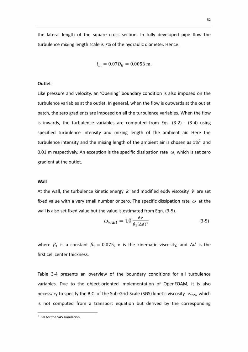
52
the lateral length of the square cross section. In fully developed pipe flow the
turbulence mixing length scale is 7% of the hydraulic diameter. Hence:
= 0.07 = 0.0056 m.
Outlet
Like pressure and velocity, an ’Opening’ boundary condition is also imposed on the
turbulence variables at the outlet. In general, when the flow is outwards at the outlet
patch, the zero gradients are imposed on all the turbulence variables. When the flow
is inwards, the turbulence variables are computed from Eqs. (3-2) - (3-4) using
specified turbulence intensity and mixing length of the ambient air. Here the
turbulence intensity and the mixing length of the ambient air is chosen as 1%1 and
0.01 m respectively. An exception is the specific dissipation rate , which is set zero
gradient at the outlet.
Wall
At the wall, the turbulence kinetic energy and modified eddy viscosity are set
fixed value with a very small number or zero. The specific dissipation rate at the
wall is also set fixed value but the value is estimated from Eqn. (3-5).
𝑤𝑎 = 106𝜈
𝛽1(Δ𝑑)2 (3-5)
where 𝛽1 is a constant 𝛽1 = 0.075, is the kinematic viscosity, and is the
first cell center thickness.
Table 3-4 presents an overview of the boundary conditions for all turbulence
variables. Due to the object-oriented implementation of OpenFOAM, it is also
necessary to specify the B.C. of the Sub-Grid-Scale (SGS) kinetic viscosity , which
is not computed from a transport equation but derived by the corresponding
1 5% for the SAS simulation.
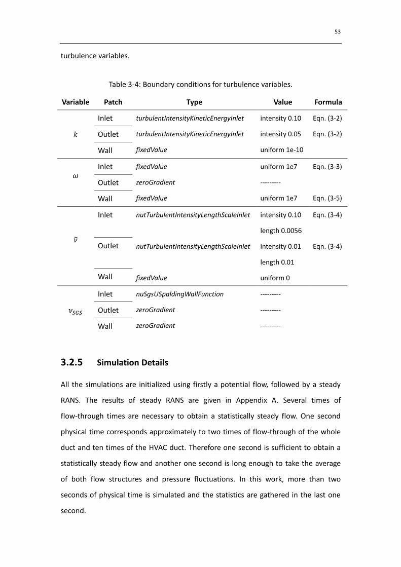
53
turbulence variables.
Table 3-4: Boundary conditions for turbulence variables.
Variable Patch Type Value Formula
Inlet turbulentIntensityKineticEnergyInlet
turbulentIntensityKineticEnergyInlet
fixedValue
intensity 0.10
intensity 0.05
uniform 1e-10
Eqn. (3-2)
Eqn. (3-2) Outlet
Wall
Inlet fixedValue
zeroGradient
fixedValue
uniform 1e7
---------
uniform 1e7
Eqn. (3-3)
Eqn. (3-5)
Outlet
Wall
Inlet
nutTurbulentIntensityLengthScaleInlet
nutTurbulentIntensityLengthScaleInlet
fixedValue
intensity 0.10
length 0.0056
intensity 0.01
length 0.01
uniform 0
Eqn. (3-4)
Eqn. (3-4) Outlet
Wall
Inlet nuSgsUSpaldingWallFunction
zeroGradient
zeroGradient
---------
---------
---------
Outlet
Wall
3.2.5 Simulation Details
All the simulations are initialized using firstly a potential flow, followed by a steady
RANS. The results of steady RANS are given in Appendix A. Several times of
flow-through times are necessary to obtain a statistically steady flow. One second
physical time corresponds approximately to two times of flow-through of the whole
duct and ten times of the HVAC duct. Therefore one second is sufficient to obtain a
statistically steady flow and another one second is long enough to take the average
of both flow structures and pressure fluctuations. In this work, more than two
seconds of physical time is simulated and the statistics are gathered in the last one
second.
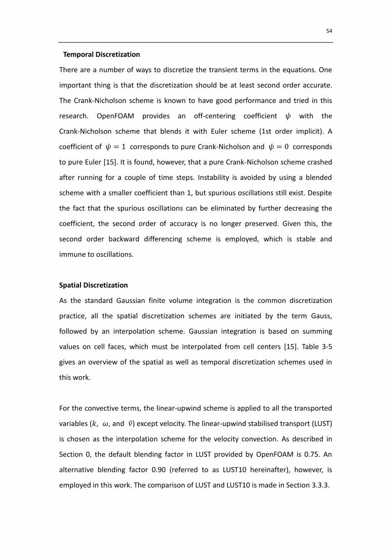
54
Temporal Discretization
There are a number of ways to discretize the transient terms in the equations. One
important thing is that the discretization should be at least second order accurate.
The Crank-Nicholson scheme is known to have good performance and tried in this
research. OpenFOAM provides an off-centering coefficient 𝜓 with the
Crank-Nicholson scheme that blends it with Euler scheme (1st order implicit). A
coefficient of 𝜓 = 1 corresponds to pure Crank-Nicholson and 𝜓 = 0 corresponds
to pure Euler [15]. It is found, however, that a pure Crank-Nicholson scheme crashed
after running for a couple of time steps. Instability is avoided by using a blended
scheme with a smaller coefficient than 1, but spurious oscillations still exist. Despite
the fact that the spurious oscillations can be eliminated by further decreasing the
coefficient, the second order of accuracy is no longer preserved. Given this, the
second order backward differencing scheme is employed, which is stable and
immune to oscillations.
Spatial Discretization
As the standard Gaussian finite volume integration is the common discretization
practice, all the spatial discretization schemes are initiated by the term Gauss,
followed by an interpolation scheme. Gaussian integration is based on summing
values on cell faces, which must be interpolated from cell centers [15]. Table 3-5
gives an overview of the spatial as well as temporal discretization schemes used in
this work.
For the convective terms, the linear-upwind scheme is applied to all the transported
variables ( , , and ) except velocity. The linear-upwind stabilised transport (LUST)
is chosen as the interpolation scheme for the velocity convection. As described in
Section 0, the default blending factor in LUST provided by OpenFOAM is 0.75. An
alternative blending factor 0.90 (referred to as LUST10 hereinafter), however, is
employed in this work. The comparison of LUST and LUST10 is made in Section 3.3.3.
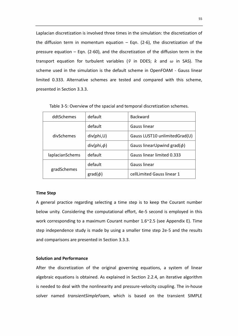
55
Laplacian discretization is involved three times in the simulation: the discretization of
the diffusion term in momentum equation – Eqn. (2-6), the discretization of the
pressure equation – Eqn. (2-60), and the discretization of the diffusion term in the
transport equation for turbulent variables ( in DDES; and in SAS). The
scheme used in the simulation is the default scheme in OpenFOAM - Gauss linear
limited 0.333. Alternative schemes are tested and compared with this scheme,
presented in Section 3.3.3.
Table 3-5: Overview of the spacial and temporal discretization schemes.
ddtSchemes default Backward
divSchemes
default Gauss linear
div(phi,U) Gauss LUST10 unlimitedGrad(U)
div(phi, ) Gauss linearUpwind grad( )
laplacianSchems default Gauss linear limited 0.333
gradSchemes default Gauss linear
grad( ) cellLimited Gauss linear 1
Time Step
A general practice regarding selecting a time step is to keep the Courant number
below unity. Considering the computational effort, 4e-5 second is employed in this
work corresponding to a maximum Courant number 1.6~2.5 (see Appendix E). Time
step independence study is made by using a smaller time step 2e-5 and the results
and comparisons are presented in Section 3.3.3.
Solution and Performance
After the discretization of the original governing equations, a system of linear
algebraic equations is obtained. As explained in Section 2.2.4, an iterative algorithm
is needed to deal with the nonlinearity and pressure-velocity coupling. The in-house
solver named transientSimpleFoam, which is based on the transient SIMPLE
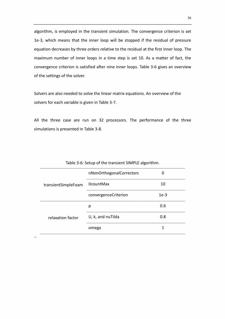
56
algorithm, is employed in the transient simulation. The convergence criterion is set
1e-3, which means that the inner loop will be stopped if the residual of pressure
equation decreases by three orders relative to the residual at the first inner loop. The
maximum number of inner loops in a time step is set 10. As a matter of fact, the
convergence criterion is satisfied after nine inner loops. Table 3-6 gives an overview
of the settings of the solver.
Solvers are also needed to solve the linear matrix equations. An overview of the
solvers for each variable is given in Table 3-7.
All the three case are run on 32 processors. The performance of the three
simulations is presented in Table 3-8.
Table 3-6: Setup of the transient SIMPLE algorithm.
transientSimpleFoam
nNonOrthogonalCorrectors 0
IIcountMax 10
convergenceCriterion 1e-3
relaxation factor
p 0.6
U, k, and nuTilda 0.8
omega 1
´´
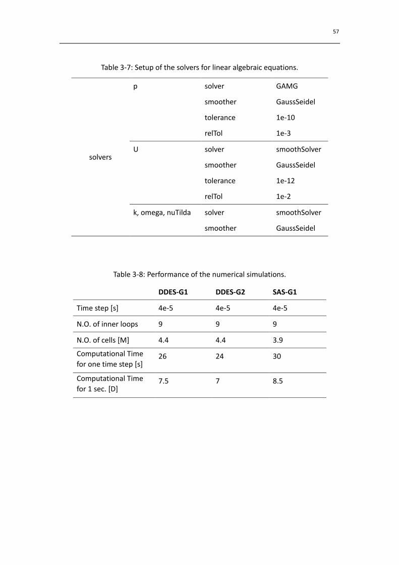
57
Table 3-7: Setup of the solvers for linear algebraic equations.
solvers
p solver
smoother
tolerance
relTol
GAMG
GaussSeidel
1e-10
1e-3
U solver
smoother
tolerance
relTol
smoothSolver
GaussSeidel
1e-12
1e-2
k, omega, nuTilda solver
smoother
smoothSolver
GaussSeidel
Table 3-8: Performance of the numerical simulations.
DDES-G1 DDES-G2 SAS-G1
Time step [s] 4e-5 4e-5 4e-5
N.O. of inner loops 9 9 9
N.O. of cells [M] 4.4 4.4 3.9
Computational Time
for one time step [s] 26 24 30
Computational Time
for 1 sec. [D] 7.5 7 8.5
58
3.3 Results and Comparisons
The numerical results of all the simulation cases as well as comparisons with
experiment are presented in this subsection. The wall pressure signals are firstly
analyzed and then the time averaged flow field is compared to the experiment. All
the time averaged results and statistical analyses are based upon the simulation in
the last one second.
3.3.1 Unsteady Pressure Fluctuations
Sound is in essence an unsteady phenomenon. As a result, unlike in general
aerodynamic applications where main attention has been paid to the integrated
quantities like drag and lift coefficients, unsteady flow phenomenon needs to be
carefully analyzed in acoustic applications of CFD.
Since only the pressure at the walls will later be fed to acoustic code to compute the
sound propagation, wall pressure signals are appropriate enough to measure the
unsteadiness of the flow. The signals are analyzed over here both in the time domain
(statistical properties) and in the frequency domain (frequency analysis).
OpenFOAM function object volProbes are installed at the same locations as in the
experimental rig to monitor and record the pressures. The function object volProbes
returns text files with discrete values per time step for the fields selected by the user
in a set of prescribed points within the mesh. Note that for incompressible flow
simulation, OpenFOAM employs the kinematic pressure with the unit [𝑚2𝑠−2], from
which the dynamic pressure1 i.e. [Pa] is recovered and used in the analysis below
and later acoustic computation.
Table 3-9 and Table 3-10 present the statistical properties of the pressure signals at
1 The dynamic pressure is recovered by multiplying the kinematic pressure by the density of the fluid, which is
1.205 kg/m3 for air in this research.
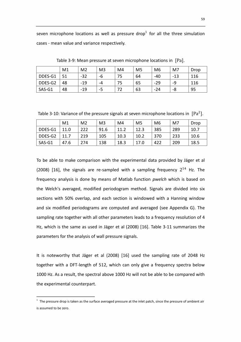
59
seven microphone locations as well as pressure drop1 for all the three simulation
cases - mean value and variance respectively.
Table 3-9: Mean pressure at seven microphone locations in [Pa].
M1 M2 M3 M4 M5 M6 M7 Drop
DDES-G1 51 -32 -6 75 64 -40 -13 116
DDES-G2 48 -19 -4 75 65 -29 -9 116
SAS-G1 48 -19 -5 72 63 -24 -8 95
Table 3-10: Variance of the pressure signals at seven microphone locations in [Pa2].
M1 M2 M3 M4 M5 M6 M7 Drop
DDES-G1 11.0 222 91.6 11.2 12.3 385 289 10.7
DDES-G2 11.7 219 105 10.3 10.2 370 233 10.6
SAS-G1 47.6 274 138 18.3 17.0 422 209 18.5
To be able to make comparison with the experimental data provided by Jäger et al
(2008) [16], the signals are re-sampled with a sampling frequency 214 Hz. The
frequency analysis is done by means of Matlab function pwelch which is based on
the Welch's averaged, modified periodogram method. Signals are divided into six
sections with 50% overlap, and each section is windowed with a Hanning window
and six modified periodograms are computed and averaged (see Appendix G). The
sampling rate together with all other parameters leads to a frequency resolution of 4
Hz, which is the same as used in Jäger et al (2008) [16]. Table 3-11 summarizes the
parameters for the analysis of wall pressure signals.
It is noteworthy that Jäger et al (2008) [16] used the sampling rate of 2048 Hz
together with a DFT-length of 512, which can only give a frequency spectra below
1000 Hz. As a result, the spectral above 1000 Hz will not be able to be compared with
the experimental counterpart.
1 The pressure drop is taken as the surface averaged pressure at the inlet patch, since the pressure of ambient air
is assumed to be zero.

60
Table 3-11: Parameters for frequency analysis.
Phys. time [s] 1
Sample rate [Hz] 214
Samples 214
FFT length 4096
Overlap 50%
Averages 6
The Matlab function pwelch returns the Power Spectra Density (PSD), while the
Sound Pressure Level (SPL) in 𝐵 is used in the comparison with measurement. SPL
can be computed from PSD through Eqn. (3-6) or Eqn. (3-7),
𝐿 = 10log [ 𝐷
𝑟𝑒𝑓2 ] (3-6)
𝐿 = 10log [ 𝐷
𝑟𝑒𝑓2 ] (3-7)
where is the reference sound pressure and is the frequency resolution.
The reference sound pressure used in this research is = 2 10−5 Pa, which is
considered as the threshold of human hearing in air, corresponding to a SPL of 0 𝐵.
In Section 3.3.1, SPL is computed based upon Eqn. (3-6), while in Section 3.3.3 SPL is
acquired from Eqn. (3-7), which is independent of frequency resolution.
Figure 3-8, Figure 3-9 and Figure 3-10 present the frequency analyses of the
unsteady wall pressure signals in the form of Sound Pressure Level (SPL) for three
simulation cases respectively. More comparisons can be found in Appendix F.
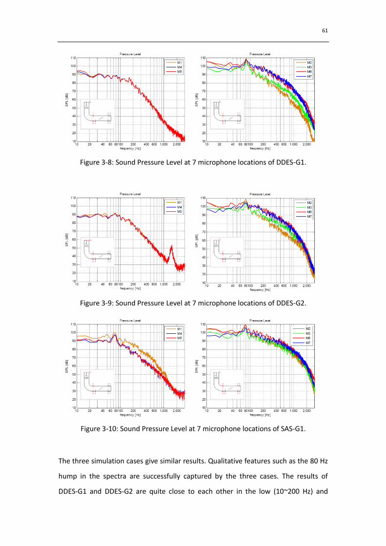
61
Figure 3-8: Sound Pressure Level at 7 microphone locations of DDES-G1.
Figure 3-9: Sound Pressure Level at 7 microphone locations of DDES-G2.
Figure 3-10: Sound Pressure Level at 7 microphone locations of SAS-G1.
The three simulation cases give similar results. Qualitative features such as the 80 Hz
hump in the spectra are successfully captured by the three cases. The results of
DDES-G1 and DDES-G2 are quite close to each other in the low (10~200 Hz) and
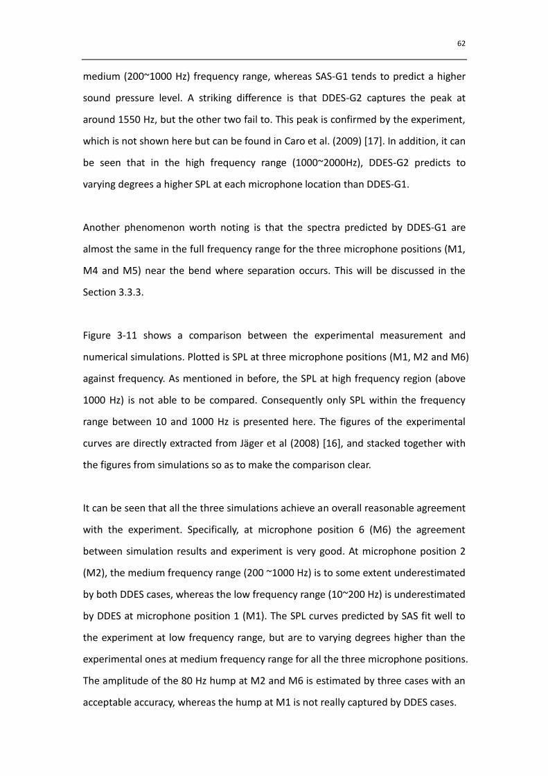
62
medium (200~1000 Hz) frequency range, whereas SAS-G1 tends to predict a higher
sound pressure level. A striking difference is that DDES-G2 captures the peak at
around 1550 Hz, but the other two fail to. This peak is confirmed by the experiment,
which is not shown here but can be found in Caro et al. (2009) [17]. In addition, it can
be seen that in the high frequency range (1000~2000Hz), DDES-G2 predicts to
varying degrees a higher SPL at each microphone location than DDES-G1.
Another phenomenon worth noting is that the spectra predicted by DDES-G1 are
almost the same in the full frequency range for the three microphone positions (M1,
M4 and M5) near the bend where separation occurs. This will be discussed in the
Section 3.3.3.
Figure 3-11 shows a comparison between the experimental measurement and
numerical simulations. Plotted is SPL at three microphone positions (M1, M2 and M6)
against frequency. As mentioned in before, the SPL at high frequency region (above
1000 Hz) is not able to be compared. Consequently only SPL within the frequency
range between 10 and 1000 Hz is presented here. The figures of the experimental
curves are directly extracted from Jäger et al (2008) [16], and stacked together with
the figures from simulations so as to make the comparison clear.
It can be seen that all the three simulations achieve an overall reasonable agreement
with the experiment. Specifically, at microphone position 6 (M6) the agreement
between simulation results and experiment is very good. At microphone position 2
(M2), the medium frequency range (200 ~1000 Hz) is to some extent underestimated
by both DDES cases, whereas the low frequency range (10~200 Hz) is underestimated
by DDES at microphone position 1 (M1). The SPL curves predicted by SAS fit well to
the experiment at low frequency range, but are to varying degrees higher than the
experimental ones at medium frequency range for all the three microphone positions.
The amplitude of the 80 Hz hump at M2 and M6 is estimated by three cases with an
acceptable accuracy, whereas the hump at M1 is not really captured by DDES cases.
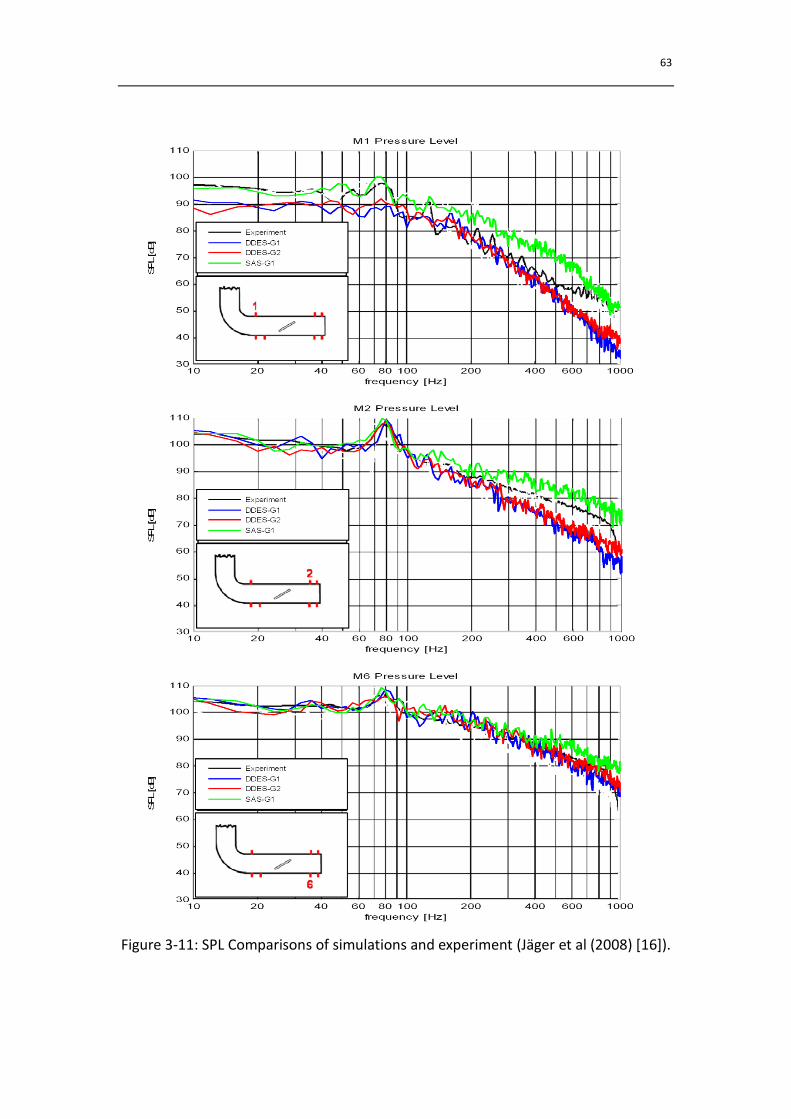
63
Figure 3-11: SPL Comparisons of simulations and experiment (Jäger et al (2008) [16]).
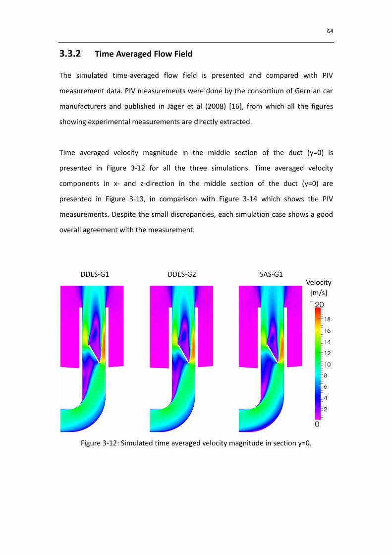
64
3.3.2 Time Averaged Flow Field
The simulated time-averaged flow field is presented and compared with PIV
measurement data. PIV measurements were done by the consortium of German car
manufacturers and published in Jäger et al (2008) [16], from which all the figures
showing experimental measurements are directly extracted.
Time averaged velocity magnitude in the middle section of the duct (y=0) is
presented in Figure 3-12 for all the three simulations. Time averaged velocity
components in x- and z-direction in the middle section of the duct (y=0) are
presented in Figure 3-13, in comparison with Figure 3-14 which shows the PIV
measurements. Despite the small discrepancies, each simulation case shows a good
overall agreement with the measurement.
Figure 3-12: Simulated time averaged velocity magnitude in section y=0.
DDES-G1 DDES-G2 SAS-G1 Velocity
[m/s]
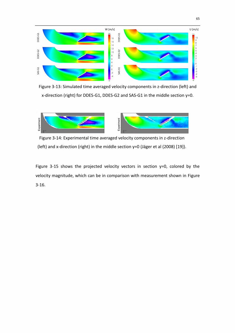
65
Figure 3-13: Simulated time averaged velocity components in z-direction (left) and
x-direction (right) for DDES-G1, DDES-G2 and SAS-G1 in the middle section y=0.
Figure 3-14: Experimental time averaged velocity components in z-direction
(left) and x-direction (right) in the middle section y=0 (Jäger et al (2008) [19]).
Figure 3-15 shows the projected velocity vectors in section y=0, colored by the
velocity magnitude, which can be in comparison with measurement shown in Figure
3-16.
W [m/s] U [m/s]
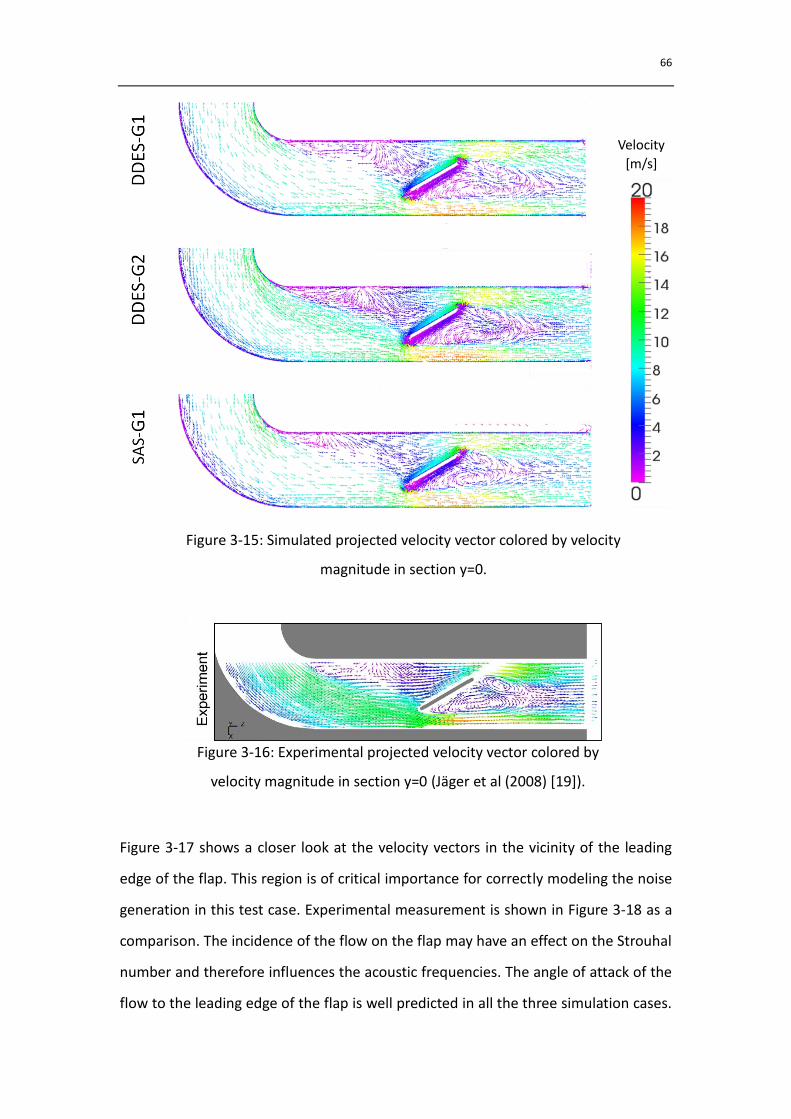
66
Figure 3-15: Simulated projected velocity vector colored by velocity
magnitude in section y=0.
Figure 3-16: Experimental projected velocity vector colored by
velocity magnitude in section y=0 (Jäger et al (2008) [19]).
Figure 3-17 shows a closer look at the velocity vectors in the vicinity of the leading
edge of the flap. This region is of critical importance for correctly modeling the noise
generation in this test case. Experimental measurement is shown in Figure 3-18 as a
comparison. The incidence of the flow on the flap may have an effect on the Strouhal
number and therefore influences the acoustic frequencies. The angle of attack of the
flow to the leading edge of the flap is well predicted in all the three simulation cases.
Velocity
[m/s]
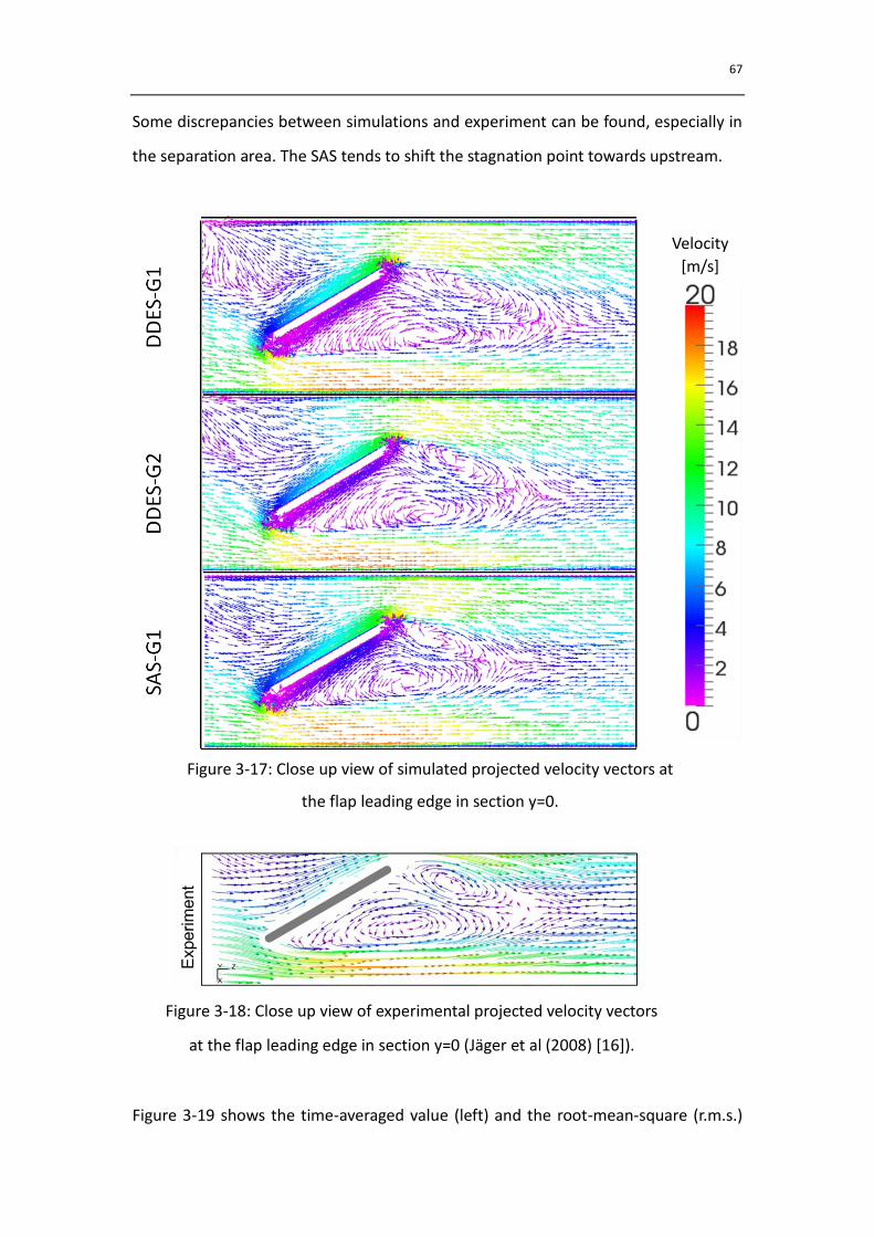
67
Some discrepancies between simulations and experiment can be found, especially in
the separation area. The SAS tends to shift the stagnation point towards upstream.
Figure 3-17: Close up view of simulated projected velocity vectors at
the flap leading edge in section y=0.
Figure 3-19 shows the time-averaged value (left) and the root-mean-square (r.m.s.)
Figure 3-18: Close up view of experimental projected velocity vectors
at the flap leading edge in section y=0 (Jäger et al (2008) [16]).
Velocity
[m/s]
68
value (middle and right) of the pressure at the duct walls. The r.m.s. value is given in
logarithmic scale (log1 𝑠). It can be seen that the estimated time-averaged
pressure is quite close to each other, while the r.m.s value of the pressure predicted
by SAS is higher than DDES cases. This higher level of r.m.s value corresponds to a
higher level of fluctuation, which has also been verified by the larger variance in
Table 3-10 and the higher SPL in Figure 3-11. Small differences between the two
DDES cases can be found by taking a closer a look at the separation region.
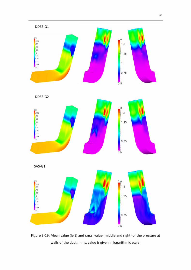
69
Figure 3-19: Mean value (left) and r.m.s. value (middle and right) of the pressure at
walls of the duct; r.m.s. value is given in logarithmic scale.
DDES-G1
DDES-G2
SAS-G1
70
3.3.3 Influence Study
The influence of alternative discretization schemes and time steps on the predicted
SPL is studied in this subsection. Please note, however, that this study is far from
thorough and conclusive. The purpose of this study is to find out an appropriate set
of parameters and schemes that would give relatively accurate results for this
particular case. General and thorough investigations are beyond the scope of this
thesis.
Convective Discretization
Central differencing scheme or CD is of second order accuracy and exhibits very low
numerical dissipation, which is often used in LES where very low numerical
dissipation is required together with very fine grid resolution to resolve the turbulent
scales [8]. CD is however reported to suffer from spurious oscillations. Therefore
blending CD with upwind or linear-upwind scheme is often necessary to guarantee
both accuracy and boundedness. The discretization scheme (interpolation scheme)
for the velocity convection used in this research is the linear-upwind stabilised
transport, which blends linear (i.e. CD) with linear-upwind. The default blending
factor of this scheme implemented in OpenFOAM is 0.75, referred to as LUST
hereinafter. However, the factor used in this research is 0.90 (hereinafter LUST10).
LUST10 weighs more of linear than LUST does, which might induce less numerical
dissipation than LUST.
LUST and LUST10 are compared in the Figure 3-20. Due to the limited time and
computational resources, the comparative simulation is based on DDES-G1 and run
for only 0.4 second, and the frequency analysis in done on the last 0.3277 second.
This period might not be long enough for averaging, but we can still gain some
insights. All other settings are equal for both LUST and LUST10.
There exist some discrepancies between LUST and LUST10. In spite of this, Figure
71
3-20 shows an overall good agreement, considering the short period for averaging.
The peaks at some frequencies predicted by LUST10 are higher than LUST, probably
due to the lower numerical dissipation of LUST10. Because of this, LUST10 is used for
the simulation.
Laplacian Discretization
As discussed in Section 0, laplacian discretization is involved three times: the
discretization of the diffusion term in momentum equation – laplacian(nu,U), the
discretization of the pressure equation - laplacian((1|A(U)),p), and the discretization
of the diffusion term in the transport equation for turbulent variables ( in DDES;
and in SAS). The scheme used in the simulation is the default scheme in
OpenFOAM - Gauss linear limited 0.333, which is a both corrected and limited
scheme. Alternative schemes are tested based on DDES-G2 and comparisons are
presented in Figure 3-21. The comparative simulation is run for 0.5 second and the
last 0.4096 second. Table 3-12 gives an overview of the schemes used for different
terms and their corresponding SPL curves in Figure 3-21.
Table 3-12: Selection for laplacian discretization schemes.
Red Line Blue Line
laplacian(nu,U) Gauss linear limited 0.333 Gauss linear uncorrected
laplacian((1|A(U)),p) Gauss linear limited 0.333 Gauss linear limited 0.2
jjDiffusion for Gauss linear limited 0.333 Gauss linear uncorrected
It is found that uncorrected schemes (indicated by blue lines) runs slightly faster than
the corrected ones (indicated by red lines), but the SPL predicted by uncorrected
schemes at microphone 2 is a little lower than the corrected schemes in the high
frequency range (100~2000 Hz).
72
Time Step
The influence of time step is studied here. A finer step =2e-5 sec is tested and
compared with =4e-5 sec based on both DDES-G1 and SAS-G1. For the
comparative simulation based on DDES-G1, the simulation runs over a period of 0.35
second with the last 0.3277 second being analyzed. For the comparative simulation
based on SAS-G1, the simulation runs for 0.22 second and the last 0.2048 second is
fed to the frequency analysis.
Error! Reference source not found. and Figure 3-23 show the comparison based on
DDES-G1 and SAS-G1 respectively. The most striking difference is the peak at around
2000 Hz which appears when the time step is 2e-5. Additional tests are executed
based on DDES-G2 with time step 2e-5 and DDES-G1 with time step 1e-5. It is found
that the peak only happens to the first grid (G1) when time step is equal or smaller
than 2e-5.
It is observed from Figure 3-22 that at microphone position 2 (M2) the SPL with time
step 2e-5 is a little higher than with time step 4e-5 in the medium frequency range.
Recall that SPL at M2 is underestimated by both DDES-G1 and DDES-G2 in the
medium frequency range relative to the experimental measurement. Therefore a
smaller time step is beneficial in terms of accuracy.
Initialization
As in DDES the switch between RANS and LES mode is to some extent solution
dependent. Therefore the initial condition might have an influence on the resolved
flow field. The initialization independence study for DDES-G1 case is conducted and
described in Appendix D. Remarkable influence is not observed. On the contrary, the
study shows that the grid G1 tends to suppress the instability of the separating flow
downstream the bend.
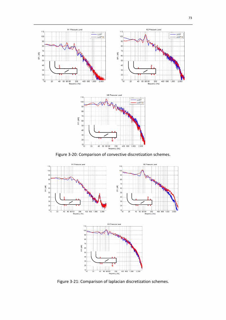
73
Figure 3-20: Comparison of convective discretization schemes.
Figure 3-21: Comparison of laplacian discretization schemes.
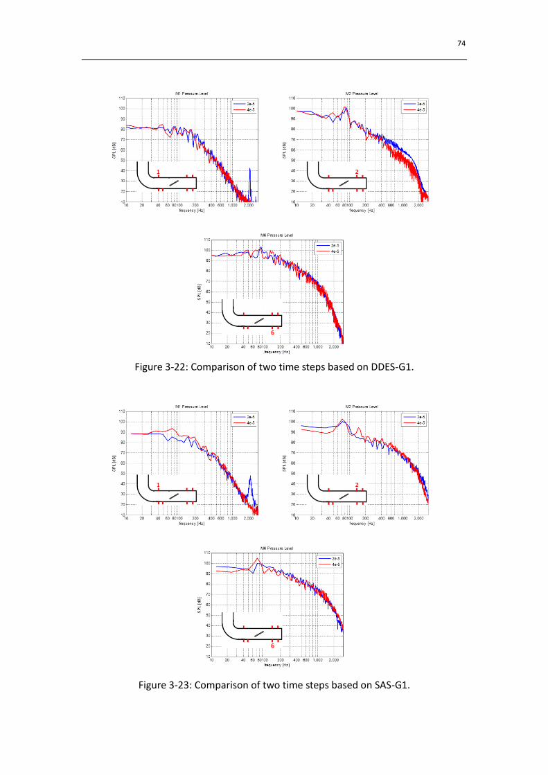
74
Figure 3-22: Comparison of two time steps based on DDES-G1.
Figure 3-23: Comparison of two time steps based on SAS-G1.
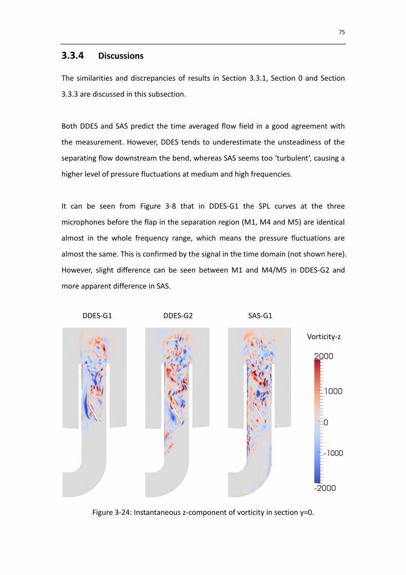
75
3.3.4 Discussions
The similarities and discrepancies of results in Section 3.3.1, Section 0 and Section
3.3.3 are discussed in this subsection.
Both DDES and SAS predict the time averaged flow field in a good agreement with
the measurement. However, DDES tends to underestimate the unsteadiness of the
separating flow downstream the bend, whereas SAS seems too ‘turbulent’, causing a
higher level of pressure fluctuations at medium and high frequencies.
It can be seen from Figure 3-8 that in DDES-G1 the SPL curves at the three
microphones before the flap in the separation region (M1, M4 and M5) are identical
almost in the whole frequency range, which means the pressure fluctuations are
almost the same. This is confirmed by the signal in the time domain (not shown here).
However, slight difference can be seen between M1 and M4/M5 in DDES-G2 and
more apparent difference in SAS.
Figure 3-24: Instantaneous z-component of vorticity in section y=0.
DDES-G1 DDES-G2 SAS-G1
Vorticity-z
76
Figure 3-24 shows the z-component of the vorticity of the three cases at the middle
pane of the duct (y=0). We can see that the shear layer separating from the elbow in
DDES-G1 is totally steady, while it is not in DDES-G2 and SAS. This can explain the
approximately identical SPL curves in DDES-G1, and might also contribute to the
slightly higher SPL of DDES-G2 in the high frequency range than DDES-G1. The same
phenomena are observed for the 3-dimentional vortical structures, presented with
Q-isosurface in Figure 3-25. The influence of initialization is also studied and
presented in Appendix D. It is found that the grid G1 tends to suppress the instability
of the separating flow downstream the bend.
From Figure 3-24 and Figure 3-25, we can see that the SAS captures much more small
turbulence structures than the other two DDES cases. In addition, the small
turbulence structures in the near wall region are also observed for the SAS case,
which should not be so obvious. The author is inclined to ascribe this to the
implementation of SAS in the current version of OpenFOAM. Therefore more
validations and verifications are necessary for SAS to be used in the future
applications.
The 1550 Hz peak which appears in DDES-G2 and also in experiment does not appear
in either DDES-G1 or SAS-G1. Instead, when the time step is 2e-5 second or even
smaller, a peak around 2000 Hz is observed in both two G1 cases (DDES and SAS). In
order to gain an insight into the influence of initialization on the final results, a test
simulation initialized by the flow field of DDES-G2 is run on the grid G1 for 0.104
second. The time step is set to 4e-5. The result is similar to DDES-G1 case and neither
the 1550 Hz peak nor 2000 Hz peak can be observed (see Appendix D). It is therefore
safe to say that grid quality is the only impact factor in this phenomenon. The author
tends to believe that the 2000 Hz peak and is in essence the same phenomenon as
the 1550 peak but shifted due to the low quality of the grid. In the meantime, as the
quality of the grid is low, finer time step is needed to capture the peak. The main
improvement of the second grid (G2) relative to the first grid (G1) lies in two aspects:
77
the refinement in the separation area and the remedy of missing layers. In order to
find out which one is decisive, a test simulation with time step equal to 2e-5 second
is done on a third grid (G3) generated based on the same setup as the first grid
(which means miss layers still exist) but with a refinement in the separation area. The
2000 Hz peak can also be observed in the test simulation (see Appendix C). Therefore
the frequency shift can be considered as the consequence of the missing layers.
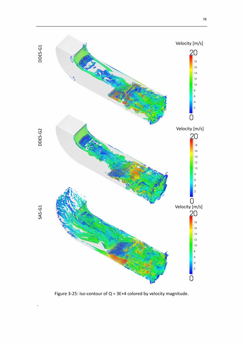
78
Figure 3-25: Iso-contour of Q = 3E+4 colored by velocity magnitude.
.
DD
ES-G
1 D
DES
-G2
SAS-
G1
Velocity [m/s]
Velocity [m/s]
Velocity [m/s]
79
4. Conclusions and Recommendations
The main purpose of this thesis is to validate the feasibility of a hybrid method in
computational aero-acoustics (CAA) to predict correctly the flow induced noise
within an HVAC system. The potential of the hybrid method has been demonstrated
in the numerical investigation of flow induced noise in a simplified HVAC duct.
Unsteady incompressible flow CFD simulation, as the first step of the hybrid method,
has been executed using hybrid RANS-LES approaches. CFD results have shown a
fairly good agreement with the measurements in terms of both time averaged flow
field and unsteady pressure fluctuations. However, some discrepancies from
measurements can be found and some issues regarding CFD simulation arises. In this
chapter, the conclusions and recommendations based on the test case are presented.
4.1 Conclusions
Two hybrid RANS-LES approaches are selected to compute the flow field which is
used to identify acoustic sources. Two grids with different local refinement and
quality are used in the numerical simulation. Influence study is also conducted to
investigate the impact of different discretization schemes and time step on the
pressure fluctuations. Some findings regarding the CFD simulation are described
below.
Both DDES and SAS approaches are able to calculate the flow over a flap successfully.
Difficulties lie mainly in the computation of weak separating flow downstream the
bend. DDES underestimates the unsteadiness of the flow in the separation area,
whereas SAS seems to be too ‘turbulent’, leading to a high level of pressure
fluctuation in the medium and high frequency range. As SAS shows obvious turbulent
structures in the near-wall region, further verification and validation are necessary
for SAS to be used in future applications.
In addition to saving the computational cost, mesh quality is of importance for the
80
prediction of some tonal noise at high frequencies. Missing layers should be avoided
and local refinement of the mesh at some critical regions is also beneficial.
Discretization schemes should be chosen to keep the numerical dissipation minimal
as long as stability is ensured. The Backward temporal differencing scheme ensures
stability but is found somewhat to smear out the solution in the long time. When
blended scheme is used for the convective discretization, central difference should
be weighted as highly as possible. Correction in the laplacian discretization shows a
positive effect on the results when the grid is non-orthogonal.
Despite the rule of thumb that the Courant number should be kept below one,
slightly coarser time step can be used to save the computational time without losing
much accuracy. However, this applies only when the Courant number in the critical
region is not above one.
4.2 Recommendations
Due to limited time and computational resources, this study cannot be thorough and
conclusive. The conclusions drawn in the previous section require more verification
and validation. Further work is thus strongly recommended. This subsection lists
some proposals for future work.
The results of acoustic computation follow the same trend as the experimental data
at medium and high frequencies, which verifies the CFD simulation. However,
discrepancies can be observed. Therefore more careful and accurate acoustic
computation needs to be conducted.
Since difficulties lie mainly in the computation of flow around the elbow, more
attention should be paid to the weak separating flow. DDES approaches based on
81
some two-equation RANS models such as − and − 𝑇 are suggested to
be tested, which in principle might give more accurate results than the original DDES.
SAS is quite a promising approach with lower computational effort than DDES.
However, the implementation of SAS − 𝑇 in OpenFOAM might need to be
examined and verification study is desirable.
The DDES approach used in this study is not simple. It is rather challenging to identify
modeling errors. It is desirous to put some efforts to the identification of LES mode
and RANS mode in the solution and the interaction between the two modes.
Despite the encouraging results, this study is done on a rather simplified HVAC duct.
Real life HVAC components are much more complex than this one. One of the
aspects of the future work is to compute a relatively simple but real HVAC
component.

82
83
Bibliography
[1] C. Wagner, T. Huttl, and P. Sagaut. Large-Eddy Simulation for Acoustics.
Cambridge University Press, 2007.
[2] S. B. Pope . Turbulent Flows. Cambridge University Press, 2000.
[3] P.R. Spalart, and S.R. Allmaras. A one-equation turbulence model for
aerodynamic flows. AIAA Paper 92-0439, 1992.
[4] P.R. Spalart and S.R. Allmaras. A one-equation turbulence model for
aerodynamics flows. La Recherche Aérospatiate, 1:5-21, 1994.
[5] F.R. Menter. Two-equation eddy-viscosity turbulence models for engineering
applications. AIAA Journal, 32:1598-1605, 1994.
[6] F.R. Menter, M. Kuntz, and R. Langtry. Ten years of industrial experience with
the SST turbulence model. Turbulence, Heat and Mass Transfer, 4:625-632,
2003.
[7] P.R. Spalart, W.-H. Jou, M. Strelets, and S.R. Allmaras. Comments on the
feasibility of LES for wings, and on a hybrid RANS/LES approach. In C. Liu and
Z. Liu, editors, Advances in DNS/LES. Greyden Press, 1997.
[8] C. Mockett, A comprehensive study of detached-eddy simulation. PhD thesis,
Technical University of Berlin, Berlin, 2009.
[9] F.R. Menter, M. Kuntz. The Aerodynamics of Heavy Vehicles: Trucks, Buses, and
Trains. Springer Verlag, 2004.
[10] P.R. Spalart. Young person’s guide to Detached Eddy Simulation grids. Technical
Report NASA/CR-2001-211032, NASA Langeley Research Center, 2001.
[11] P.R. Spalart, S. Deck, M.L. Shur, K.D. Squires, M.K. Strelets, and A. Travin. A
new version of detached-eddy simulation resistant to ambiguous grid densities.
Theoretical and Computational Fluid Dynamics, 20:181-195, 2006.
[12] H. Werner, B. Marianna, and R. Alistair. DESider – A European Effort on Hybrid
RANS-LES Modelling. Springer, 2009.
[13] H.K. Versteeg, and W. Malalasekera. An Introduction to Computational Fluid
Dynamics – The Finite Volume Method. Pearson Education, 2007.
[14] H. Jasak. Error analysis and estimation in the finite volume method with
applications to fluid flows, PhD theiss, University of London, Imperial College,
London, 1996.
[15] OpenFOAM User Guid. version 2.1.1. OpenFOAM Foundation, 2012.
84
[16] A. Jäger, F. Decker, M. Hartmann, M. Islam, T. Lemke, J. Ocker, V. Schewarz, F.
Ullrich, B. Crouse, G. Balasubramanian, F. Mendonca, and R. Drobietz.
Numerical and experimental investigation of the noise generated by a flap in a
simplified HVAC duct. AIAA Paper 2008-2902, 2008.
[17] S. Caro, Y. Detandt, J. Manera, R. Toppinga, and F. Mendonca. Validation of a
new hybrid CAA strategy and application to the noise generated by a flap in a
simplified HVAC duct. AIA Paper 2009-3352, 2009.
[18] C. Carton de Wiart, P. Geuzaine, Y. Detandt, J. Manera, S. Caro, Y. Marichal, and
G. Winckelmans. Validation of a hybrid CAA method: noise generated by a flap
in a simplified HVAC duct. AIAA Paper 2010-3995, 2010.
[19] P. Martinez-Lera, R. Hallez, H. Bériot, and C. Schram. Compuation of sound in
a simplified HVAC duct based on aerodynamic pressure. AIAA Paper
2012-2070, 2012.

85
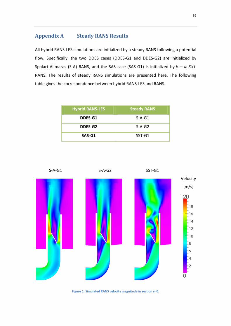
86
Appendix A Steady RANS Results
All hybrid RANS-LES simulations are initialized by a steady RANS following a potential
flow. Specifically, the two DDES cases (DDES-G1 and DDES-G2) are initialized by
Spalart-Allmaras (S-A) RANS, and the SAS case (SAS-G1) is initialized by
RANS. The results of steady RANS simulations are presented here. The following
table gives the correspondence between hybrid RANS-LES and RANS.
Hybrid RANS-LES Steady RANS
DDES-G1 S-A-G1
DDES-G2 S-A-G2
SAS-G1 SST-G1
Figure 1: Simulated RANS velocity magnitude in section y=0.
S-A-G1 S-A-G2 SST-G1
Velocity
[m/s]
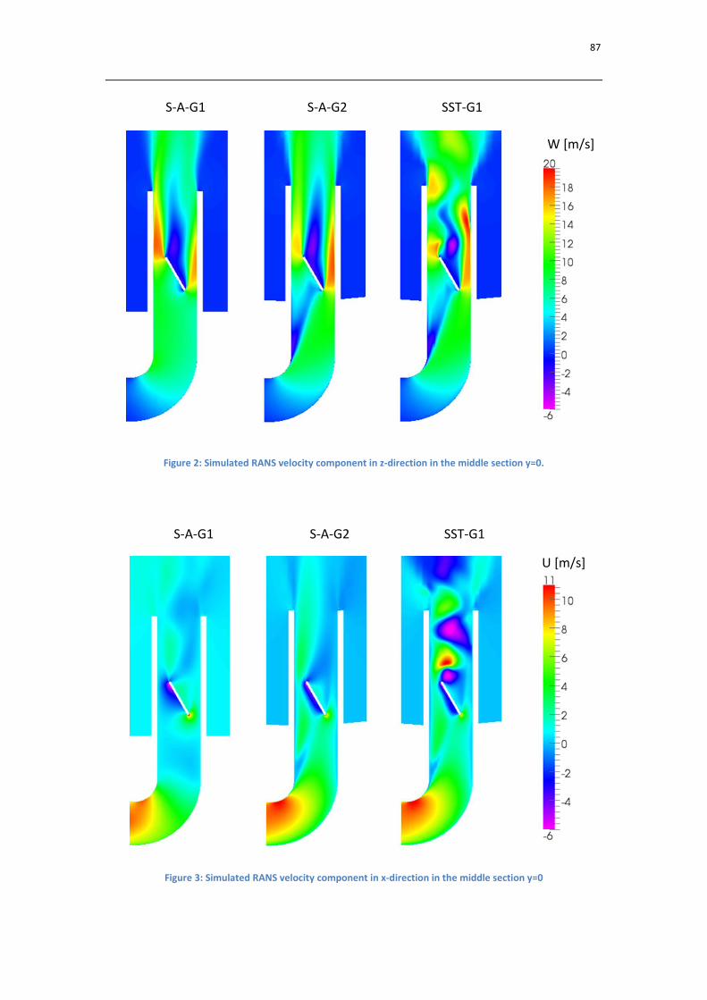
87
Figure 2: Simulated RANS velocity component in z-direction in the middle section y=0.
Figure 3: Simulated RANS velocity component in x-direction in the middle section y=0
S-A-G1 S-A-G2 SST-G1
S-A-G1 S-A-G2 SST-G1
W [m/s] U [m/s]
U [m/s]
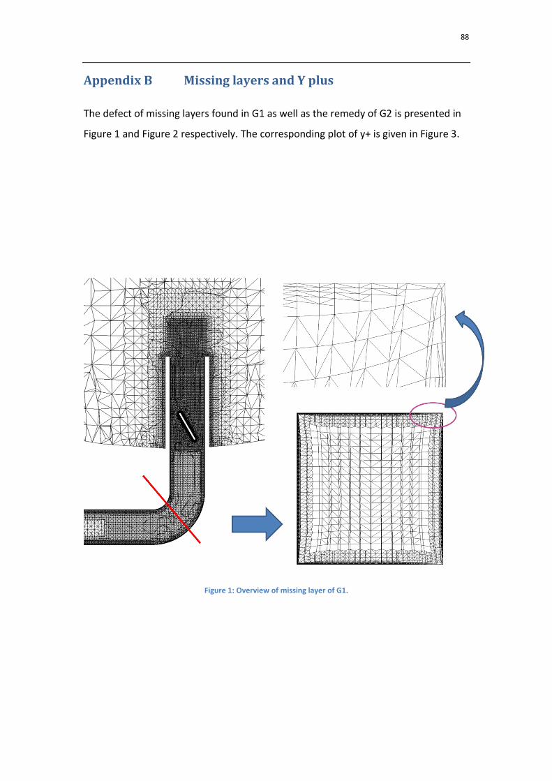
88
Appendix B Missing layers and Y plus
The defect of missing layers found in G1 as well as the remedy of G2 is presented in
Figure 1 and Figure 2 respectively. The corresponding plot of y+ is given in Figure 3.
Figure 1: Overview of missing layer of G1.
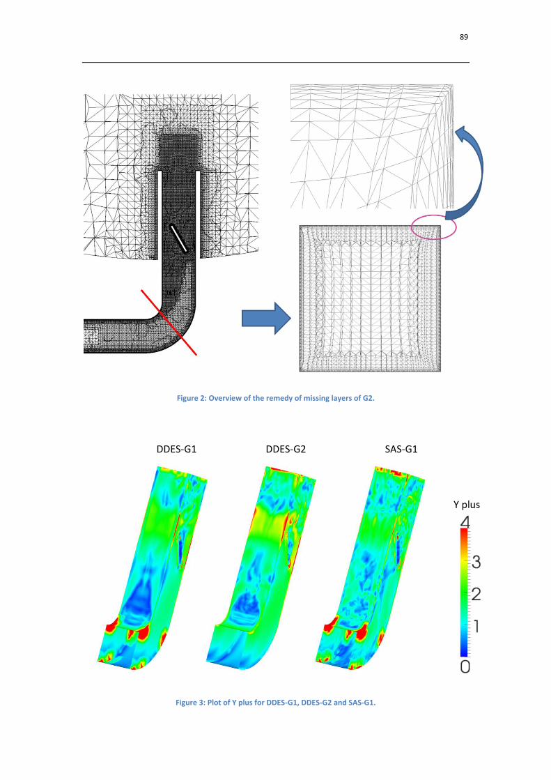
89
Figure 2: Overview of the remedy of missing layers of G2.
Figure 3: Plot of Y plus for DDES-G1, DDES-G2 and SAS-G1.
DDES-G1 DDES-G2 SAS-G1
Y plus
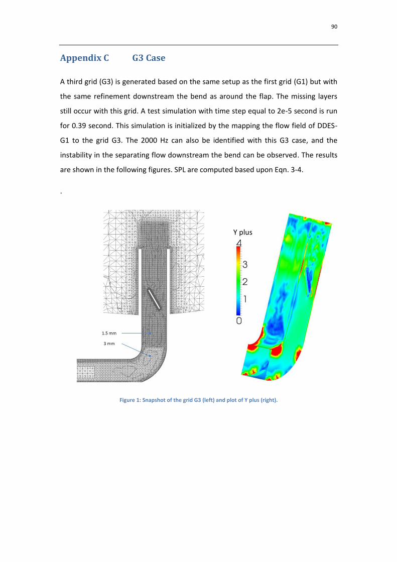
90
Appendix C G3 Case
A third grid (G3) is generated based on the same setup as the first grid (G1) but with
the same refinement downstream the bend as around the flap. The missing layers
still occur with this grid. A test simulation with time step equal to 2e-5 second is run
for 0.39 second. This simulation is initialized by the mapping the flow field of DDES-
G1 to the grid G3. The 2000 Hz can also be identified with this G3 case, and the
instability in the separating flow downstream the bend can be observed. The results
are shown in the following figures. SPL are computed based upon Eqn. 3-4.
.
Figure 1: Snapshot of the grid G3 (left) and plot of Y plus (right).
Y plus
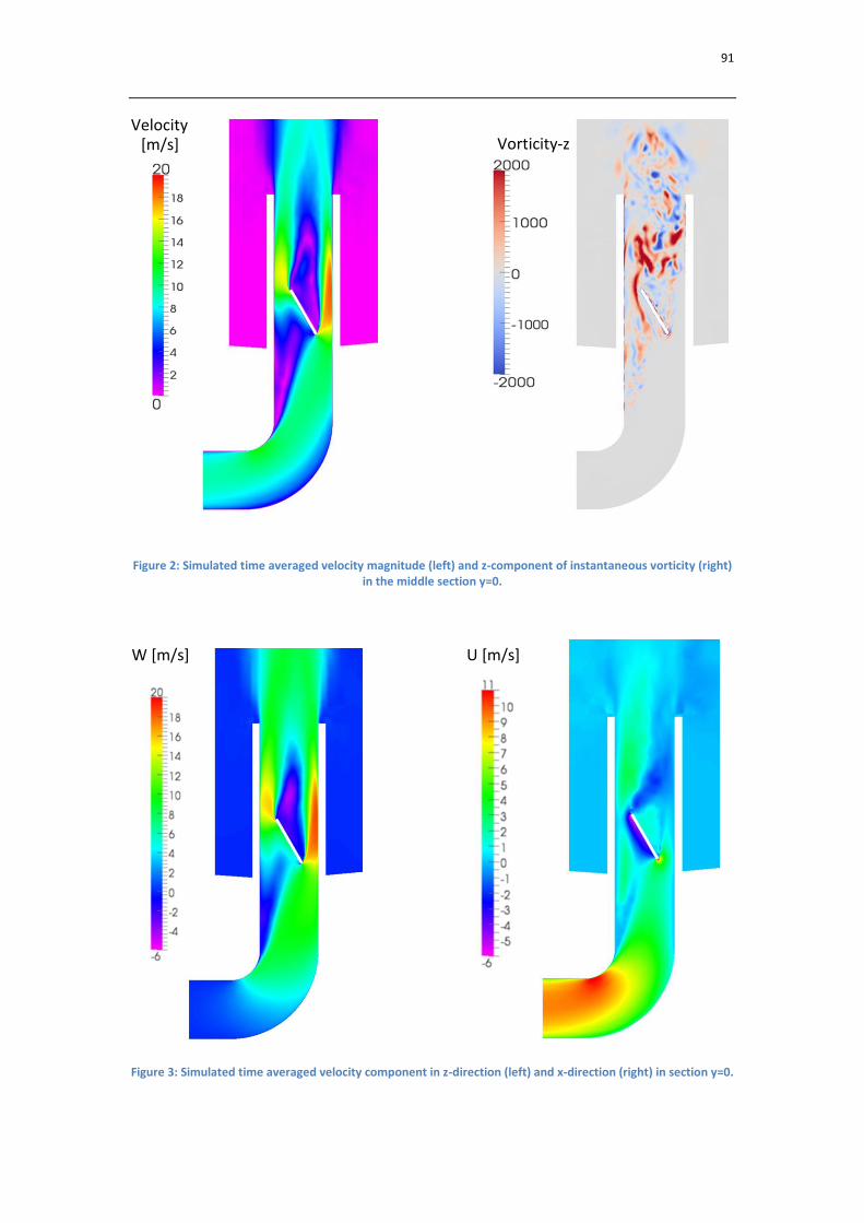
91
Figure 2: Simulated time averaged velocity magnitude (left) and z-component of instantaneous vorticity (right) in the middle section y=0.
Figure 3: Simulated time averaged velocity component in z-direction (left) and x-direction (right) in section y=0.
Velocity [m/s] Vorticity-z
W [m/s] U [m/s]
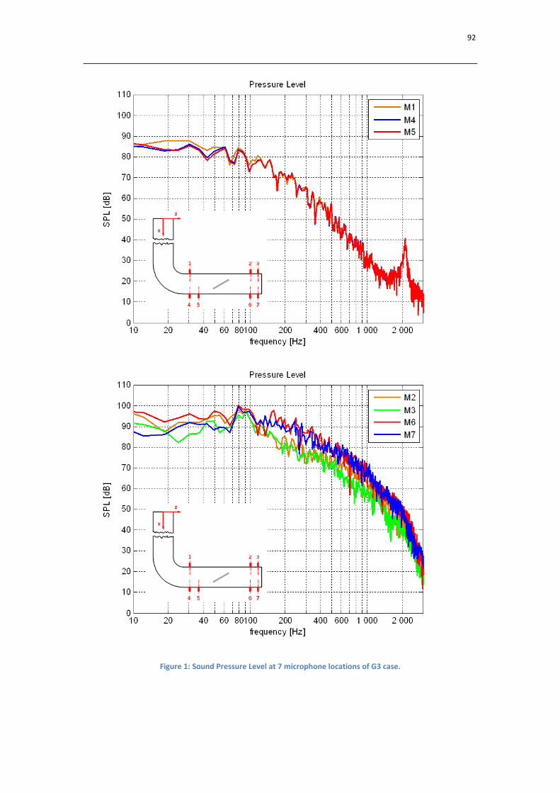
92
Figure 1: Sound Pressure Level at 7 microphone locations of G3 case.

93
Appendix D Initialization Independence
In order to gain an insight into the influence of initialization on the final results, a
test simulation initialized by the flow field of DDES-G2 is run on the grid G1 for 0.104
second. The time step is set to 4e-5. The result is similar to DDES-G1 case and neither
the 1550 Hz peak nor 2000 Hz peak can be observed. It is found that the instability of
separating flow downstream the bend is suppressed by the grid. Figure 1 shows the
z-component of instantaneous vorticity in middle section y=0 at the start time t=0
(left) and the end time t=0.104 (right).
Figure 1: Instantaneous z-component of vorticity in section y=0: left t=0; right t=0.104.
Vorticity-z
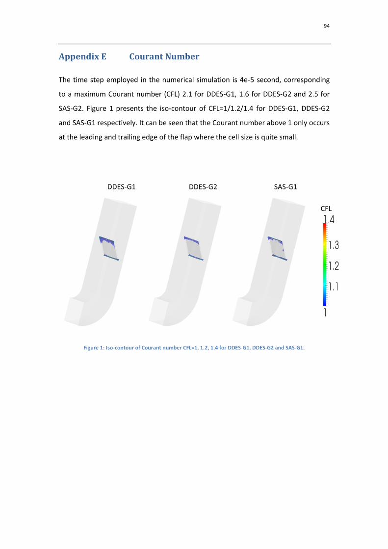
94
Appendix E Courant Number
The time step employed in the numerical simulation is 4e-5 second, corresponding
to a maximum Courant number (CFL) 2.1 for DDES-G1, 1.6 for DDES-G2 and 2.5 for
SAS-G2. Figure 1 presents the iso-contour of CFL=1/1.2/1.4 for DDES-G1, DDES-G2
and SAS-G1 respectively. It can be seen that the Courant number above 1 only occurs
at the leading and trailing edge of the flap where the cell size is quite small.
Figure 1: Iso-contour of Courant number CFL=1, 1.2, 1.4 for DDES-G1, DDES-G2 and SAS-G1.
DDES-G1 DDES-G2 SAS-G1
CFL
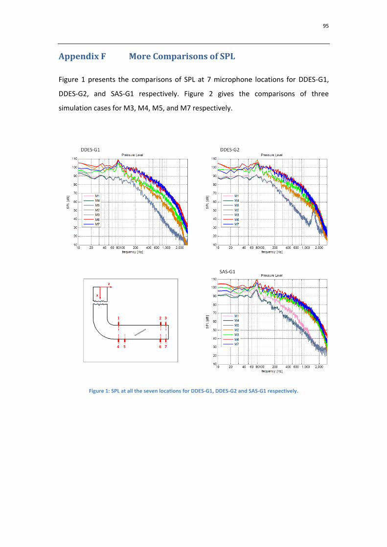
95
Appendix F More Comparisons of SPL
Figure 1 presents the comparisons of SPL at 7 microphone locations for DDES-G1,
DDES-G2, and SAS-G1 respectively. Figure 2 gives the comparisons of three
simulation cases for M3, M4, M5, and M7 respectively.
Figure 1: SPL at all the seven locations for DDES-G1, DDES-G2 and SAS-G1 respectively.

96
Figure 2: Comparison of SPL at M3, M4, M5, and M7.
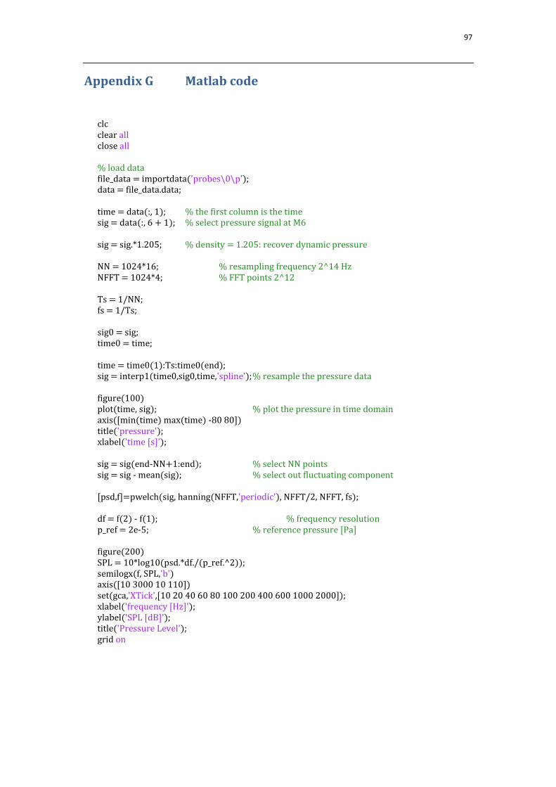
97
Appendix G Matlab code
clc clear all close all % load data file_data = importdata('probes\0\p'); data = file_data.data; time = data(:, 1); % the first column is the time sig = data(:, 6 + 1); % select pressure signal at M6 sig = sig.*1.205; % density = 1.205: recover dynamic pressure NN = 1024*16; % resampling frequency 2^14 Hz NFFT = 1024*4; % FFT points 2^12 Ts = 1/NN; fs = 1/Ts; sig0 = sig; time0 = time; time = time0(1):Ts:time0(end); sig = interp1(time0,sig0,time,'spline'); % resample the pressure data figure(100) plot(time, sig); % plot the pressure in time domain axis([min(time) max(time) -80 80]) title('pressure'); xlabel('time [s]'); sig = sig(end-NN+1:end); % select NN points sig = sig - mean(sig); % select out fluctuating component [psd,f]=pwelch(sig, hanning(NFFT,'periodic'), NFFT/2, NFFT, fs); df = f(2) - f(1); % frequency resolution p_ref = 2e-5; % reference pressure [Pa] figure(200) SPL = 10*log10(psd.*df./(p_ref.^2)); semilogx(f, SPL,'b') axis([10 3000 10 110]) set(gca,'XTick',[10 20 40 60 80 100 200 400 600 1000 2000]); xlabel('frequency [Hz]'); ylabel('SPL [dB]'); title('Pressure Level'); grid on