NUMERICAL INVESTIGATION OF BOUNDARY LAYER DETACHMENT BY ACTIVE FLOW CONTROL

Karunakaran Hemrijicks(a), Tonino Sophy(b), Julien Jouanguy(c), Arthur Da Silva(d), Luis Lemoyne(e)

(a) (b) (c) (d) (e)DRIVE – ISAT EA 1859, 49, Rue Mademoiselle Bourgeois, 58000 NEVERS, FRANCE

(a)joe.karna90@gmail.com , (b)tsophy@u-bourgogne.fr , (c)julien.jouanguy@u-bourogne.fr , (d)arthur.da-silva@u-bourgogne.fr , (e)luis.le-moyne@u-bourgogne.fr .

ABSTRACT After decades of investigations have failed to produce a positive outcome on flow control technologies that requires complex devices and micro-plumbing, recent technologies like synthetic jets, DBD (Dielectric Barrier Discharge) seems to be promising and these technologies can overcome limitations of the old ones. Our work mainly deals with delaying boundary layer detachment of over an aerodynamic body (Air foil). In this paper we produce our study of an active flow control device over the BL detachment point over a circular cylinder by the aid of simulations. Results from the uncontrolled flow seem to be in accordance with literature and the presence of the jet has an effect on the boundary layer.

Keywords: Detachment point control, Flow control technologies, Synthetic jets and Boundary layer.

1. INTRODUCTION Boundary layer is formed when a fluid is obstructed by the body. This thin layer is formed due to the viscous friction of the adjacent layers of the fluid. This boundary layer detaches from the body when the pressure gradient is adverse (Prandtl 1904). Adverse pressure gradient and its effect on the detachment are explained in fig 1.

Figure 1 Pressure gradient and BL detachment

This detachment may be avoided or delayed when the transition occurs from laminar to turbulent boundary layer. Since turbulent boundary layer creates more friction drag than laminar, there is a need for new technologies for manipulating detachment of this boundary layer (David C Hazen 1962). The manipulation may be done by mixing or reenergizing a boundary layer. In other words low momentum bottom layers are replaced by higher momentum fluid streams

so that the boundary layer detachment is delayed or avoided.

Though for nearly a century has been spent to improve the energetic of automobiles and aircrafts. Many innovations and technologies have been developed to make the vehicle more energy efficient. The detachment occurs due to the shape of the body (a sharp edge or rear end). In commercial vehicles like trucks body have improved aerodynamically to reduce the drag (Ola Logdberg 2008). In motorsport aerodynamics is more crucial to push the vehicle ahead of current performance. In aviation apart from these aerodynamic developments in the body there is a need for technologies like flow control devices that induces primary vortex that energizes boundary layer and delays the detachment. These devices are classified in to two categories:

1. Passive devices (fig 2) are mechanical devices or alterations made on the exterior body of the vehicle. These devices create stream wise vortices that convert the low momentum fluid layers with free stream so that to influence adverse pressure gradient and delay BL detachment. Rigidity in the control and drag penalty are the drawbacks.

Figure 2 Passive Vortex Generator

2. Active devices are technologies integrated on the body.

Recent experiments show that passive devices have better performances than active devices but they have drag penalties and they are not controlled according to the requirement (Godard et al 2006a, b and c).

Proc. of the Int. Workshop on Simulation for Energy, Sustainable Development & Environment 2014, 978-88-97999-42-3; Bruzzone, Cellier, Janosy, Longo, Zacharewicz Eds.

20

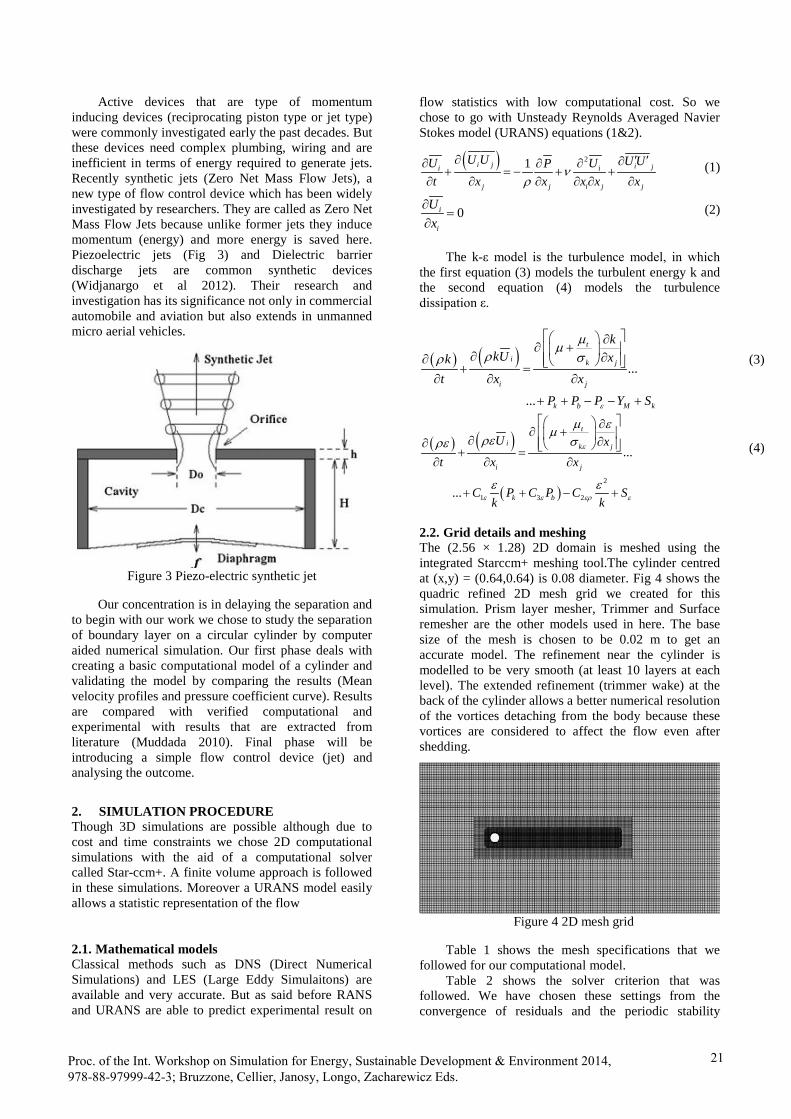
Active devices that are type of momentum inducing devices (reciprocating piston type or jet type) were commonly investigated early the past decades. But these devices need complex plumbing, wiring and are inefficient in terms of energy required to generate jets. Recently synthetic jets (Zero Net Mass Flow Jets), a new type of flow control device which has been widely investigated by researchers. They are called as Zero Net Mass Flow Jets because unlike former jets they induce momentum (energy) and more energy is saved here. Piezoelectric jets (Fig 3) and Dielectric barrier discharge jets are common synthetic devices (Widjanargo et al 2012). Their research and investigation has its significance not only in commercial automobile and aviation but also extends in unmanned micro aerial vehicles.

Figure 3 Piezo-electric synthetic jet

Our concentration is in delaying the separation and to begin with our work we chose to study the separation of boundary layer on a circular cylinder by computer aided numerical simulation. Our first phase deals with creating a basic computational model of a cylinder and validating the model by comparing the results (Mean velocity profiles and pressure coefficient curve). Results are compared with verified computational and experimental with results that are extracted from literature (Muddada 2010). Final phase will be introducing a simple flow control device (jet) and analysing the outcome.

2. SIMULATION PROCEDURE Though 3D simulations are possible although due to cost and time constraints we chose 2D computational simulations with the aid of a computational solver called Star-ccm+. A finite volume approach is followed in these simulations. Moreover a URANS model easily allows a statistic representation of the flow 2.1. Mathematical models Classical methods such as DNS (Direct Numerical Simulations) and LES (Large Eddy Simulaitons) are available and very accurate. But as said before RANS and URANS are able to predict experimental result on

flow statistics with low computational cost. So we chose to go with Unsteady Reynolds Averaged Navier Stokes model (URANS) equations (1&2).

( ) 21i j i ji i

j j i j j

U U U UU UPt x x x x x

νρ

∂ ′ ′∂∂ ∂∂+ = − + +

∂ ∂ ∂ ∂ ∂ ∂ (1)

0i

i

Ux

∂=

∂ (2)

The k-ε model is the turbulence model, in which

the first equation (3) models the turbulent energy k and the second equation (4) models the turbulence dissipation ε.

( ) ( )...

...

t

i k j

i j

k b M k

kkU xk

t x xP P P Y Sε

µµρ σρ

∂∂ + ∂ ∂∂ + =

∂ ∂ ∂

+ + − − +

(3)

( ) ( )

( )2

1 3 2

...

...

t

i k j

i j

k b

U xt x x

C P C P C Sk k

ε

ε ε ερ ε

µ εµρε σρε

ε ε

∂∂ + ∂ ∂∂ + =

∂ ∂ ∂

+ + − +

(4)

2.2. Grid details and meshing The (2.56 × 1.28) 2D domain is meshed using the integrated Starccm+ meshing tool.The cylinder centred at (x,y) = (0.64,0.64) is 0.08 diameter. Fig 4 shows the quadric refined 2D mesh grid we created for this simulation. Prism layer mesher, Trimmer and Surface remesher are the other models used in here. The base size of the mesh is chosen to be 0.02 m to get an accurate model. The refinement near the cylinder is modelled to be very smooth (at least 10 layers at each level). The extended refinement (trimmer wake) at the back of the cylinder allows a better numerical resolution of the vortices detaching from the body because these vortices are considered to affect the flow even after shedding.

Figure 4 2D mesh grid

Table 1 shows the mesh specifications that we followed for our computational model.

Table 2 shows the solver criterion that was followed. We have chosen these settings from the convergence of residuals and the periodic stability

Proc. of the Int. Workshop on Simulation for Energy, Sustainable Development & Environment 2014, 978-88-97999-42-3; Bruzzone, Cellier, Janosy, Longo, Zacharewicz Eds.

21

obtained by parameters of the model like drag coefficient and frequency of the simulation.

Table 1: Mesh details

Specifications

No.of.cells 18220 No.of faces 36434

Table 2: Simulation details

Specifications

Residuals ε<10-5 No.of.Iterations per time steps

50

No.of.Time steps 1000

2.3. Physical and boundary conditions Incompressible flow and a Reynolds number of 3900 was selected. A velocity flow inlet, pressure outlet, wall boundary for cylinder and slip walls (zero stress walls) are the boundary conditions applied to the model (fig 5). In other words slip walls are free stream velocities which means no physical boundary is formed by the slip walls. The velocity of the flow is calculated from Reynolds number (Re) 3900. The pressure outlet is modelled to maintain relative pressure zero at the outlet so that the flow leaves the boundary to maintain the atmospheric conditions at the outlet. On the cylinder no slip boundary conditions are applied.

Figure 5 Boundary conditions

3. SIMULATION AND RESULTS

3.1. Simulation and validation of cylinder model Many researchers have chosen many shapes of model like a bump or a backward facing step but we chose cylinder because it is a model that exhibits a wide range of compartment and has both favourable and adverse (unfavourable) pressure gradient which will be interesting to study. Availability of several experimental results for example in (Muddada 2010) was also a motivation.

3.1.1. Results To validate our control free model we have to compare our various outputs like mean velocities, pressure coefficient curve, vorticity field and velocity field to reference results.

Fig. 6 which represents the evolution of the pressure forces coefficient for Re = 3900, shows that the periodic flow is reached at our simulation final time.

The main frequency of 2 Hz corresponds to a Strouhal

number 0

0.21Freq DSt

V⋅

= = .

Figure 6 Cxp evolution without control

Comparison with some Strouhal numbers mentioned in (Muddada2010) is related in table 3. Standard k-ε numerical model of Muddada et al. and experimental results of Kravchenko et al. (Kravchenko2000) are mentioned.

Table 3: Strouhal numbers Strouhal number for Re = 3900

Present study 0.21 Muddada2010 k-ε 0.22 Kravchenko exp. 0.21

The obtained result seems to be in accordance with

reference Strouhal number.

3.1.1.1. Pressure Coefficient Pressure coefficient is a parameter to quantify the velocity distribution over a body.

02

00.5pP PC

Vρ−

=⋅ ⋅

(5)

Where: P – Static pressure at point of interest P0 – Static pressure at free stream ρ – Free stream density V0 – Free stream velocity In Fig 7 shows the comparison of pressure

coefficient curve of our simulation with experimental and simulation result extracted form reference literature. From the Cp curve, we can witness the detachment point around 90° of theta. Regarding fig 7 in the case of uncontrolled flow, our 2D U-RANS solution seems to be a few closer to the experimental results of Kravchenko et al. (Kravchenko2000) than k-ε numerical results of Muddada et al. (Muddada 2010).

Proc. of the Int. Workshop on Simulation for Energy, Sustainable Development & Environment 2014, 978-88-97999-42-3; Bruzzone, Cellier, Janosy, Longo, Zacharewicz Eds.

22

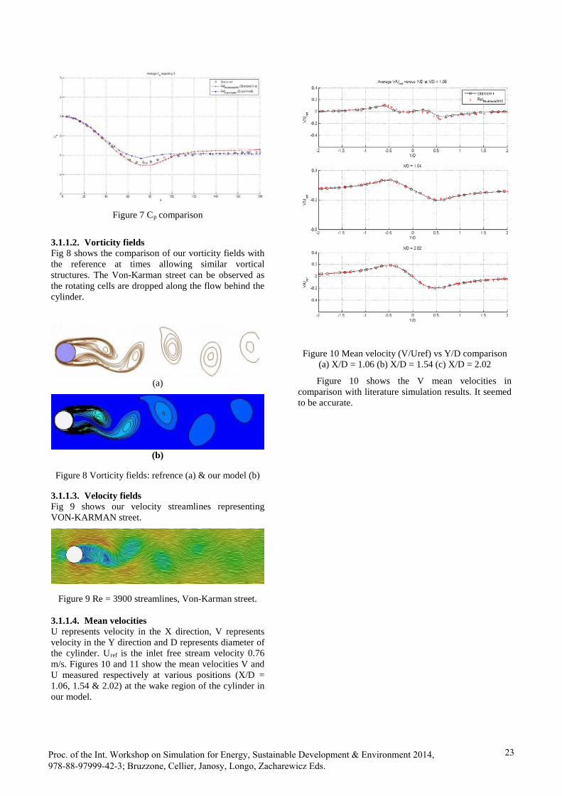
Figure 7 Cp comparison

3.1.1.2. Vorticity fields Fig 8 shows the comparison of our vorticity fields with the reference at times allowing similar vortical structures. The Von-Karman street can be observed as the rotating cells are dropped along the flow behind the cylinder.

(a)

(b)

Figure 8 Vorticity fields: refrence (a) & our model (b)

3.1.1.3. Velocity fields Fig 9 shows our velocity streamlines representing VON-KARMAN street.

Figure 9 Re = 3900 streamlines, Von-Karman street. 3.1.1.4. Mean velocities U represents velocity in the X direction, V represents velocity in the Y direction and D represents diameter of the cylinder. Uref is the inlet free stream velocity 0.76 m/s. Figures 10 and 11 show the mean velocities V and U measured respectively at various positions (X/D = 1.06, 1.54 & 2.02) at the wake region of the cylinder in our model.

Figure 10 Mean velocity (V/Uref) vs Y/D comparison (a) X/D = 1.06 (b) X/D = 1.54 (c) X/D = 2.02

Figure 10 shows the V mean velocities in comparison with literature simulation results. It seemed to be accurate.

Proc. of the Int. Workshop on Simulation for Energy, Sustainable Development & Environment 2014, 978-88-97999-42-3; Bruzzone, Cellier, Janosy, Longo, Zacharewicz Eds.

23

(a)

(b)

(c)

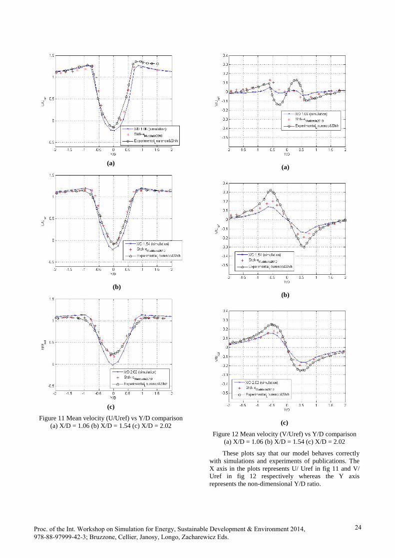
Figure 11 Mean velocity (U/Uref) vs Y/D comparison (a) X/D = 1.06 (b) X/D = 1.54 (c) X/D = 2.02

(a)

(b)

(c)

Figure 12 Mean velocity (V/Uref) vs Y/D comparison (a) X/D = 1.06 (b) X/D = 1.54 (c) X/D = 2.02

These plots say that our model behaves correctly with simulations and experiments of publications. The X axis in the plots represents U/ Uref in fig 11 and V/ Uref in fig 12 respectively whereas the Y axis represents the non-dimensional Y/D ratio.

Proc. of the Int. Workshop on Simulation for Energy, Sustainable Development & Environment 2014, 978-88-97999-42-3; Bruzzone, Cellier, Janosy, Longo, Zacharewicz Eds.

24

3.1.2. Comments Our simulation results such the Cp curve, velocity fields and vorticity fields are proved to behave close to Standard k-ε models and the experimental results used in the publication (Muddada2010).

There are some differences in experimental curve due to unavoidable external disturbance during experiments (as observed in Muddada 2010).

Mean values of the velocities are taken as the instantaneous velocities around the cylinder and are non-symmetrical due to vortex shedding at the wake.

From the three U mean velocities (Fig 11) we can witness the accuracy of our model to the publication. As we see our results at X/D = 2.02 are quite different from Std K-ε model than X/D =1.06 and 1.54. These inaccuracies can be corrected further making some improvements like using finer mesh or another wall model. The shape of the U mean velocities is due to the recirculation at the wake of the cylinder. The minimum value of the velocity increases from X/D = 1.06 to X/D = 2.02 due to the dissipation of vortices. We can also witness the same mechanism in the V mean velocity curve. From V mean velocity curve for X/D = 1.06 we can see that there is a region of flat zero velocity after the positive bump. This null velocity region is produced as a result of suction produced by wake. 3.2. Implementing a flow control device A simple flow control device is introduced to affect BL detachment. We created a normal jet at θ = 90° with a velocity of 7.6 % of the maximum flow velocity. This jet can be seen in Fig. 13 placed on top of the cylinder.

Figure 13 Velocity Vector in presence of jet

Fig. 14 which represents the evolution of the pressure force coefficient shows that the periodic flow is reached. The main frequency is 1.63 Hz, corresponding to a Strouhal number of 0.17.

Thus, all the average values are calculated on one unique period.

Figure 14 Cxp evolution with top jet

Fig 15 compares our Cp curve for the model with

jet with the model which has no jet. The jet introduction seems to alter the condition here. First we can see that Cp curve is no longer symmetrical. The jet introduction at the top of the cylinder involves a separation between the upper and lower sides. So, one can see two Cp curves in case of jet introduction. For the upper side of new curve the Cp deviates from previous case by, at a first time, reaching a lower value.

Figure 15 Cp curve with jet vs without jet

This is due to the increase in momentum caused by

the increment of the velocity due to the jet. Even if the curve tends to reach the original one, one can see near 90°, the presence of the discontinuity make it decrease again. As a result the pressure is generally lower with the jet. This is the sign of delay in detachment. The second Cp curve is the pressure coefficient at the bottom of the cylinder. The bottom Cp curve is much decreased and it is linked to the acceleration occurring at the bottom of the cylinder. This can be witnessed in Fig 13 showing a fluid acceleration just at the bottom of the circular object. Moreover, the stagnation point is shifted above (Fig 15). This non-symmetry is due to the presence of a single jet at the top. This drawback can be corrected during future works by introducing another jet at the bottom or a periodic pulsed jet.

Proc. of the Int. Workshop on Simulation for Energy, Sustainable Development & Environment 2014, 978-88-97999-42-3; Bruzzone, Cellier, Janosy, Longo, Zacharewicz Eds.

25

Figure 16 Cp curve with jet vs without jet

As the 90° jet creates the effects of a virtual wall, it

was decided to test a new position at 120°. In figure 16 instead of superposing the upper and lower Cp between 0° and 180°, the curves are now deployed until 360°. The new jet at 120° tends to accelerate the flow compared to the 90° jet, and discontinuities are attenuated. Further works will treat the case of 2 opposite jets, to respect cylinder symmetry. 4. CONCLUSION A 2D numerical study on the effect of flow control over a circular cylinder has been conducted using URANS Starccm+ CFD software model.

A validation test on the flow without control is performed at Re = 3900. Results seem to be accurate compared to numerical and experimental data from the literature. The detachment point figures to be near 90° which is a value close to theoretical angle of 80°.

Then a normal velocity jet is introduced at the top of the cylinder. Several effects are observed due to the presence of jet. Detachment point is moved from its original location. This outcome is encouraging for future work. A control of the detachment point is similar to controlling drag or lift in the flow. Repercussions on energy consumption could be figured. Next work can introduce a second jet at the bottom of the cylinder permitting the flow symmetry. The direction of the inlet fluid jet can also be improved and more generally a parametrical study on the jet characteristic can be conducted.

REFERENCES Godard, G., Stanislas, J.M, 2006a. Control of a

decelerating boundary layer. Part 1: Optimization of passive vortex generators. Aerospace science and technology, 10, 181–191.

Godard, G., Stanislas, M., Foucaut, J.M, 2006b. Control of a decelerating boundary layer. Part 2: Optimization of slotted jets vortex generators. Aerospace science and technology, 10, 394–400.

Godard, G., Stanislas, J.M, 2006c. Control of a decelerating boundary layer. Part 3: Optimization

of round jets vortex generators. Aerospace science and technology, 10, 455–464.

Hazen C David, 1965. Boundary layer control. Princeton, Princeton University.

Kravchenko, A.G., Moin, P., 2000. Numerical studies of flow over a circular cylinder at ReD = 3900. Physics of Fluids, 12 (2), 403–417.

Muddada, S and Patnaik, B.S.V, 2010. An assessment of turbulence models for the prediction of flow past a circular cylinder with momentum injection. Journal of wind engineering and industrial aerodynamics, 575-591.

Ola, L., 2008. Vortex generators and turbulent boundary layer separation control. Technical reports from Royal Institute of Technology, KTH Mechanics, Stockholm, Sweden.

Prandtl, L, 1904. Boundary layer theory. Verhandlungen des dritten internationalen Mathematiker-Kongresses, Heidelberg, GERMANY.

Widjanarki, M.D., Geesing, J.A.K, Vries H, Hoeijmakers, W.M., 2012. Experimental/Numerical investigatin airfoil with flow control by synthetic jets. 28th International congress of the Aeronautical science.

Proc. of the Int. Workshop on Simulation for Energy, Sustainable Development & Environment 2014, 978-88-97999-42-3; Bruzzone, Cellier, Janosy, Longo, Zacharewicz Eds.

26