ELSEVIER Performance Evaluation 3 1 (1998) 229-243

Numerical inversion of multidimensional Laplace transforms

by the Laguerre method

Joseph Abate a, Gagan L. Choudhury b,l, Ward Whitt ‘,* a 900 Hammond Road, Ridgewood, NJ 074.50-2908, USA

b AT&T Laboratories, Room IL-238, Holmdel, NJ 07733-3030, USA ’ AT&TLubs-Research, 180 Park Avenue, Florham Park, NJ 07932-0971, USA

Received 15 July 1995; received in revised form 29 November 1996

Abstract

Numerical transform inversion can be useful to solve stochastic models arising in the performance evaluation of telecom- munications and computer systems. We contribute to this technique in this paper by extending our recently developed variant of the Laguerre method for numerically inverting Laplace transforms to multidimensional Laplace transforms. An important application of multidimensional inversion is to calculate time-dependent performance measures of stochastic systems. Key features of our new al,gorithm are: (1) an efficient FFT-based extension of our previously developed variant of the Fourier- series method to calculate the coefficients of the multidimensional Laguerre generating function, and (2) systematic methods for scaling to accelerate convergence of infinite series, using Wynn’s c-algorithm and exploiting geometric decay rates of Laguerre coefficients. These features greatly speed up the algorithm while controlling errors. We illustrate the effectiveness of our algorithm through numerical examples. For many problems, hundreds of function evaluations can be computed in just a few seconds. 0 1998 Published by Elsevier Science B.V.

Keywords: Numerical transform inversion; Laplace transforms; Multidimensional Laplace transforms; Laguerre polynomials; Weeks’ algorithm; Fast Fourier transform; Accelerated summation; Wynn’s 6-algorithm

1. Introduction

In this paper we develop an effective algorithm for numerically inverting multidimensional Laplace transforms by the Laguerre method. This paper is a sequel to our previous paper [l] in which we de- veloped a new variant of the Laguerre method for numerically inverting one-dimensional Laplace trans- forms. Other one-dimensional variants of the Laguerre method are the original (1966) Weeks [ 181 algorithm and ACM Algorithm 662 in Garbow et al. [9,10]. Another variant of the Laguerre method

* Corresponding author. Tel.: +l 908 582 6484; fax: +1 908 582 2379; e-mail: wow@research.att.com. ’ E-mail: gagan@bu~ckaroo.att.com.

0166-5316/98/$19.00 0 1998 Published by Elsevier Science B.V. All rights reserved PIZ SOl66-5316(9’7)00002-3

230 J. Abate et al. /Pelformance Evaluation 31 (1998) 229-243

for multidimensional Laplace transforms has recently been proposed by Moor-thy [ 1 l] (which came to our attention while this paper was under review). The general approach here is the same as in [ 1 l] and as in previous one-dimensional algorithms such as [ 1,9,10,18], but there are important differences in implementation.

We are interested in multidimensional transform inversion because it allows us to calculate quantities of interest in many important stochastic models arising in the performance analysis of telecommunications and computer systems. Examples include time-dependent performance of stationary and non-stationary systems [5] and joint distributions in polling models [6]. Our algorithm here provides an alternative to the Fourier-series algorithm for inverting multidimensional Laplace transforms developed in [4]. (Another variant of the Fourier-series method for multidimensional Laplace transforms recently has been presented by Moorthy [ 121.) As in the one-dimensional case, our experience is that the Fourier-series method tends to be more robust (i.e., works for a larger class of functions without special tuning), but the Laguerre method can be very fast for well-behaved functions, especially when function values are sought for a large number of arguments.

For simplicity, we consider only the bivariate case, but the algorithm extends directly to n-dimensional functions. Thus, our goal is to calculate values of a real-valued function f defined on the positive quadrant of the plane, rW$ = [0, oo) x [0, oo), by numerically inverting its Laplace transform

0003

h s2) = ss

edS1t1’S2’2)f(tl, t2) dtt dt2,

0 0

(1)

which we assume is well-defined, e.g., convergent and thus analytic for Re(st) > 0 and Re(q) > 0; e.g.,

see [8] or [17]. The basis for our inversion algorithm is the classical Laguerre-series representation of f, which we re-

view in Section 2. We review how to compute the Laguerre functions in Section 3. In Section 4 we develop an efficient algorithm to compute the Laguerre coefficients. It is based on the multidimensional generating function inversion algorithm developed in [4], but greatly speeds it up through several modifications, in- cluding a fast-Fourier-transform (FF T) implementation. In Section 5 we develop scaling and summation acceleration techniques, extending those in [l], to speed up the convergence of the Laguerre series. In Section 6 we give numerical examples from queueing theory illustrating the algorithm. In particular, we calculate the complementary cumulative distribution function (tail probability) of the time-dependent work- load (virtual waiting time) in the transient M/G/l queue with various service-time distributions. Finally, in Section 7 we summarize the algorithm.

2. Laguerre-series representation

As indicated in Section 1, OUT goal is to compute values of a bivariate function f from its two-dimensional Laplace transform p in (1). To do so, we exploit a connection between the Laplace transform f^ and the generating function of the coefficients of the Laguerre-series representation of f.

For two dimensions, the classical Laguerre-series representation takes the form

f(t17 t2) = F yj at,,F&l Wnp(t2), tl 2 0 and t2 2 0, n1=0n2=0

J. Abate et al./Pe$ofomzance Evaluation 31 (1998) 229-243

where

231

Z,(t) = e+/2L,(t), t >_ 0, (3)

(4)

and

with L,(t) in (4) being the Laguerre polynomials, Z,(t) in (3) the associated Laguerre functions, qnl,n2

in (2) the Laguerre coejkients and Q (z 1,z2) in (5) the Luguerre generating function.

The key connection between the Laguerre-series representation and the Laplace transform fA is of course (5). The Laguene-series representation of f can serve as a basis for inverting its Laplace trans- form f” in (1) because the Laguerre generating function Q in (5) is expressed directly in terms of the Laplace transform ,p. This occurs because the nth Laguerre function has the Laplace transform

co

i,(s) c J e-“‘&(t) dt = 2(2s - 1)‘/(2s + l)nf’.

0

By (l), (2) and (6), the Laplace transform can be expressed as

(2Sl - l)n’ (2s2 - 1)“2

hy s2) = 4 2 fY qnlm (ZSl + 1p+l (Zs2 + 1)“2+l. n1=0n2=0

By using the conformal mapping

(Zl, z2> = Vh), T(S2)), (Sl, s2) = u+Zl), 73Z2N

with

T(s) 2s - 1 1+z

Z = = -- ri!s + 1’

s = T-‘(z) = 2(1 _ z).

(7)

(8)

(9)

we obtain (5) from (7). We can now summarize the algorithm. By (5), the Laplace transform f^ enables us to obtain the Laguerre

generating function. We then invert the generating function to obtain the Laguerre coefficients qnl ,n2. The Laguerre coefficients plus the Laguerre functions 1, in (3) enable us to compute the desired function values

f 01, t2) via (2).

The bivariate Laguerre-series representation was considered by Sumita and Kijima [lo], but they did not present an algorithm for computing the Laguerre coefficients q,, I ,n2 from the Laplace transform, which is the major contribution of this paper.

Formula (2) implies that the mathematical basis for the inversion algorithm is the theory of orthogonal polynomials. The product Laguerrefinctions I,, (tl)ln2 (t2) form an orthonormal basis for the Hilbert space L2 ( W$ , R) of square integrable real-valued functions on W$, with the inner product

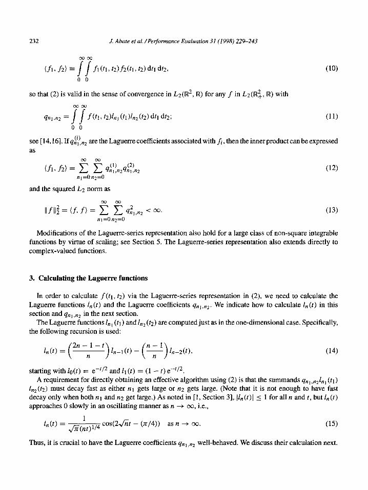
232 J. Abate et al./Performance Evaluation 31(1998) 229-243

(10)

so that (2) is valid in the sense of convergence in L2(R2, R) for any f in Lz(@, R) with

%1,n2 = ss

f(t17 td&tl (tl)&(td dtl dt2; (11)

0 0

see [14,16].If&ll:‘,n2 are the Laguerre coefficients associated with fi, then the inner product can be expressed as

00 00

(12) n1=Oq=O

and the squared L:! norm as

Ilfll; = u-3 f) = E y-J 4n2,,n2 < 00. nl=On2=0

(13)

Modifications of the Laguerre-series representation also hold for a large class of non-square integrable functions by virtue of scaling; see Section 5. The Laguerre-series representation also extends directly to complex-valued functions.

3. Calculating the Laguerre functions

In order to calculate f(tl, t2) via the Laguerre-series representation in (2), we need to calculate the Laguerre functions In(t) and the Laguerre coefficients qnr,nz. We indicate how to calculate l,,(t) in this section and qn, ,n2 in the next section.

The Laguerre functions Z,, (tl) and In2 (t2) are computed just as in the one-dimensional case. Specifically, the following recursion is used:

(14)

starting with lo(t) = e-‘j2 and Zr (t) = (1 - t) e-‘/‘. A requirement for directly obtaining an effective algorithm using (2) is that the summands qnl,n21n, (tl)

Zn2(t2) must decay fast as either nr gets large or n2 gets large. (Note that it is not enough to have fast decay only when both nr and n2 get large.) As noted in [l, Section 31, Iln(t)( 5 1 for all IZ and t, but In(t) approaches 0 slowly in an oscillating manner as n + 00, i.e.,

b(t) = 1

z/TZ(nt) V4 cos(2&t - (n/4)) as n + co. (15)

Thus, it is crucial to have the Laguerre coefficients qnl ,n2 well-behaved. We discuss their calculation next.

J. Abate et al./Pelformance Evaluation 31 (1998) 229-243 233

4. Algorithm to compute the Laguerre coefficients

Since the decay of 1, (t) with n is very slow, in order to have an effective algorithm, qnl ,n2 must decay fast as either ~11 gets large or n2 gets large. However, in many cases qnl,n2 obtained from Q (z 1, ~2) in (5) may not actually decay fast with both n 1 and n2. This difficulty is addressed in Section 5. In some cases the slow convergence may be handled by appropriately scaling Q(z1, ~2). In other cases a summation acceleration technique applied to the double infinite sum (2) greatly improves the accuracy. A combination of scaling and summation acceleration should handle most of these problems.

Computation of (ln 1 ,n2 requires the double inversion of the bivariate generating function Q(zr , ~2) given in (5). This we do by applying the Fourier-series based inversion algorithm given in [4, Section 31.

4.1. Fourier-series algorithm

Through a slight modification of Eq. (3.5) in [4], we get the approximation

qnl.nz x 9nl,q G LUW&rl, w>l+ (-l>"lRe[&-r~,mdl~ rnlryl

@1/2)-l

+ c Re[exp(-2niknl/ml)Q(rl e2nik’m1, nz)],

where i = fl,

k=l

exp(--2rikn2/m2) Q<zl, r2 e 2nik/nq)

and the resulting aliasing error is given by

ea E &z,n2 - qn,n2 = jml km2

qnl+jrnl.tq+knqrl r2 .

(16)

(17)

(18) j=O k=O

j+k>O

If ]4nl+jmi,n2+km2 ] ( C for each j, k combination appearing in (18) and if we choose r-1 = 10-Ai~mi and r2 = 10-A2/m2, then it can be shown that the aliasing error is bounded by

C( I o-A1 + lo-AZ) leaI i (1_1O_A,)(l _ 10_A2) e C(lO-A1 + 10eA2). (19)

The aliasing error may be effectively controlled by choosing A 1 and A2 large, provided that C is not large. Typically, Al = 111 and A2 = 13 are sufficient for good accuracy.

In [4] we chose ml = 211n 1 and m2 = 2Zyz2, where Zi is a roundoff error control parameter. (To be consistent with [4-l, we retain the same notation; these are not the Laguerre functions Z,(t) in (3).) The roundoff error may be reduced by increasing the parameters 11 and Z2. Typically, Z2 = 2 and 11 = 1 or 2 are sufficient for good accuracy. The above choice with mj changing with nj for j = 1 and 2 is appropriate if we need inversion at only a few points. However, in the current context, qnl ,n2 has to be computed for all nl, n2 in the range 0 5 nl 5 Nl - 1 and 0 5 n2 I N2 - 1, i.e., at a total of Nr N2 points, where Nr and N2 have to be sufficiently large so that accurate evaluation of the double infinite sum in (2) is possible

234 J. Abate et al. /Pe$ormance Evaluation 31 (1998) 229-243

using qnl,n2 only in the above range, using either truncation or a summation acceleration technique to be described in Section 5.

In the current context, we obtain a better algorithm by fixing m 1 and m2, i.e., by making mi independent of ni. Specifically, we choose ml = 2ZtNr and m2 = 2Z2N2 for all 121, n2 in the range 0 5 121 5 N1 - 1 and 0 5 n2 5 N2 - 1. At first sight, this choice might seem inefficient, since by looking at (16) and (17), we see that with mj = 2Zjnj, the total number of summations performed is

NI-l N2-l

cc 11 N2N2

212n2(11nt + 1) x ’ * 21 2 for large Nt, N2. n1=1 q=l

By contrast, the number of summations performed with the choice mj = 21j Nj is

N1-1 N2-1

cc 212N2(IlNl + 1) x 2ElZ2NfN; for large Nl, N2, n1=1 n2=1

which is four times as much as in the first case. A similar difference exists in the number of multiplications as well. However, the main computational advantage comes from the fact that, with constant ml and m2, Q(z1, ~2) needs to be computed at the same set of points for all choices of nt, n2. If we compute the Q(z1 , ~2) values once and store them for later use, then great computational saving results. Specifically, with the choice mj = 2Zjnj, the number of times Q(zr , z.2) needs to be computed is

Nl-1 N2-1

cc 2/2n2(11n1 + 1) 21 ll12N:N;

n1=1 n2=1 2 -

By contrast, with constant ml and m2, the number of times Q(zr , ~2) needs to be computed is 212N2

(ItNl + 1) F=Z 221/2Nr N2. This is a substantial savings for large Nt and N2. However, we also need a storage of 21112Nt N2 complex quantities. With today’s computers, this is usually not a problem, even with Nl = N2 = 128andll =Z2=2.

Besides the great savings in the computation of Q(zr , z2), further savings comes from an efficient (211 N1 x 212 N2)-term bivariate FFI implementation for evaluating the double sum given by (16) and (17), which we describe later. It is well known (see, e.g., [13]) that the computational complexity of such an algorithm is about 411/2Nt N2 log2(2Zl Nr ) log2(2Z2 N2), which for large Nl and N2 will be substantially less than the computational complexity of the mj = 2njlj algorithm, given by Zt12NfNi/2. However, the FFT implementation increases the required storage further to 41112 Nt N2. We summarize the performance of the proposed FFT-based algorithm for computing 4nl,n2 and compare it to the algorithm from [4] in Table 1.

Table 1 A comparison of the FFI’-based algorithm and the direct Fourier-series algorithm from [4] for calculating the Laguerre coefficients qn, ,n2 from Q(zI, ~2)

Performance measure Algorithm in [4] The new FFT-based algorithm

Number of times Q(z1, Z-J needs to be computed

Computational complexity of other computations

Storage

= 1112N;N;/2

= 1112N;N,2/2

None

= 21112 N1 N2

= 41112N1 N2 log(211 N1) log(212n2)

= 411 N112N2

J. Abate et al./Pe#onnance Evaluation 31 (1998) 229-243 235

An interesting point to note is that in the algorithm in [4] qnl,n2 is not computable if either nt = 0 or

n2 = 0, so that we have to use other techniques in those cases. However, with mj = 2Zj Nj no such alternate algorithm is needed when one or both nj’s are 0.

4.2. Error analysis of the new algorithm

The basic equations (16)-(19) still hold with the understanding that mj = 2Zj Nj instead of 2Zjnj for j = 1 and 2. In the aliasing error expression (19), note that qn,,nz appears only for either nt > Nl or n2 > N2. However., qn,,np has to be small when either nt > Nt or n2 > N2 in order for us to be able to compute the double infinite sum in (2) with only Nt and N2 terms for the two indices. This implies that

the quantity C in (19) should be small and the aliasing error will be controlled pretty tightly. In fact, the C in the new algorithm will typically be much smaller than the C in the algorithm in [3] and this is another minor advantage of the new algorithm.

Next, let US turn to the roundoff error. Define 1; = mj/2nj = Zj Nj/nj > Zj . For the new algorithm, the

parameter 2; will control the roundoff error. Since Ii > lj, the new algorithm should have less roundoff error than the algorithm in [4]. Of course, the absolute roundoff error is lower bounded by the machine precision.

4.3. FFT-based algorithm

For efficient FFI implementation, we assume that Nt , It, m 1, N2,Z2 and m2 are all nonnegative powers of 2, with mi = 2Zi Ni as before. For example, we may choose Nl = 128,Zl = 1, N2 = 64,12 = 2. This would give ml = m2 = 256. At first rewrite (16) and (17) as follows:

qn1.n2 = --$T mF1 exp(- 2niknl/m1)~(rl e2rriklm1, n2), k=O

n 2nikn2/m2)Q(zl, r2 e2Rik’m2). (21)

Now define the (ml x m2)-dimensional sequences {anl,n2} and {bnl,n2} as follows, allowing nl to range fromOtomt - 1 andn2 torangefromOtom2 - 1:

an,,n2 =4n,,n,,ry’r12, ,. (22)

b nl,n2 = Q(rl e2ninl/ml, r2 e2nin2/m2)_ (23)

Note that anl,n2 anid qnl,n2 are only defined in the range 0 5 nt I Nl - 1,O ( n2 5 N2 - 1. We extend the definition over the larger range 0 5 n1 5 ml - 1,O 5 n2 5 m2 - 1 by the inverse discrete Fourier transform (IDFT) relation

anl,n2 = 2; :g’z’exp (_?f$!!! _ F) bj,k,

which follows from (20) and (21).

(24)

236 J. Abate et al. /Performance Evaluation 31(1998) 229-243

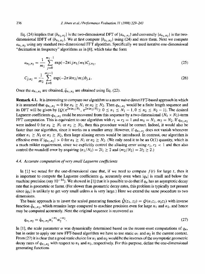
Eq. (24) implies that {bnl,nz } is the two-dimensional DFT of {a,,,,z) and conversely {an,,n2} is the two- dimensional IDFT of {bnl,n2}. We at first compute {bnl,n2} using (24) and store them. Next we compute

a,, ,n2 using any standard two-dimensional FFT algorithm. Specifically we used iterative one-dimensional “decimation in frequency” algorithms as in [S], which take the form

mz-1

C. - _!- c exp(-2nikn2/m2)bj,k. J’n2 - m2 ,&

(25)

(26)

Once the a,, ,n2 are obtained, Grill ,n2 are obtained using Eq. (22).

Remark 4.1. It is interesting to compare our algorithm to a more naive direct FFT-based approach in which

it is assumed that qnl ,n2 = 0 for 1z1 2 N1 or n2 2 N2. Then qnl,n2 would be a finite length sequence and

its DFT will be given by { Q( e2ninllNI, e2Kin2/N2 ): 0 5 n1 5 N1 - 1,O ( n2 5 N2 - 1). The desired

Laguerre coefficients qn, ,n2 could be recovered from this sequence by a two-dimensional (Nt x N2)-term

FFT computation. This is equivalent to our algorithm with rl = r-2 = 1 and ml = N1, m2 = NT. If qnl,n2

were indeed 0 for 1z1 > Nr or n2 > N2, then this procedure would be correct. Indeed, it would also be faster than our algorithm, since it works on a smaller array. However, if qnl,n2 does not vanish whenever either nl 2 Nr or n2 2 N2, then large aliasing errors would be introduced. In contrast, our algorithm is effective even if lqnl ,n2 1 > 0 for nl > N1 or n2 2 N2. (We only need it to be an 0( 1) quantity, which is a much milder requirement, since we explicitly control the aliasing error using rr , r-2 -e 1 and then also control the roundoff error by requiring (rtr/Nr) = 211 2 2 and (m2/N2) = 212 12.)

4.4. Accurate computation of very small Luguerre c0efJicient.s

In [l] we noted for the one-dimensional case that, if we need to compute f(t) for large t, then it is important to compute the Laguerre coefficients qn accurately even when lqn 1 is small and below the machine precision (say 10-14). We showed in [I] that it is possible to do that if qn has an asymptotic decay rate that is geometric or faster. (For slower than geometric decay rates, this problem is typically not present since lqn I is unlikely to get very small unless n is very large.) Here we extend the same procedure to two dimensions.

The basic approach is to invert the scaled generating function &z, 1,,3) = Q(ozl z 1, a2.z~) with inverse function &l,n2, which remains large compared to machine precision even for large n1 and n2, and hence may be computed accurately. Next the original sequence is recovered as

n -n1 4n1,n2 = 4n,,n2a1

-n2 9 . (27)

In [ 11, the scale parameter (II was dynamically determined based on the recent-most computations of qn, but in order to apply our new FFT-based algorithm we have to use static al and (~2 in the current context. From (27) it is clear that a good static choice for err and CY~ would be the inverses of the asymptotic geometric decay rates of qn, ,n2 with respect to n 1 and n2, respectively. For this purpose, define the one-dimensional generating functions

J. Abate et al. /Performance Evaluation 31 (1998) 229-243 237

(28)

(29)

The generating functions Q(zr , ~22) and Q(nr , ~2) may be obtained by one-dimensional inversion of Q(z1, ~2). Let Q(1. n2) and Q(nr , 1) have geometric decay rates as follows:

Q(l, n2) =a2,6i2 + 0(/$*) as n2 + co, (30)

Q(nt, 1) =a1,6~’ + @;I’) as rzt + 00. (31)

We suggest using al = l/B1 and cq = l/b2 as static scale factors. These decay rates can be found using inversion, as in [3]. For further discussion of scaling to compute very small function values, see [7].

5. Scaling and summation acceleration

If 4n,,n2 does not decay fast with both nl and n2, then often it is possible to speed up convergence working with the scaled function

by

h(tl, t2) = h(t1, t2; bl, b2, q, 4 = e-(a1t1+u22’2)f(tl/bl, t2/b2)

for positive real numbers bl , b2,q and a~. Clearly, h has Laplace transform

kl, ~2; bl, h 01,022) = W2.h + al%, (~2 + 02)b2).

If we can calculate h by numerically inverting k, then we can recover f from h by setting

f(tl, t2) = eo1b1r+u2b2th(bltl, b&; bl, b2, CT~,CQ).

The Laguerre generating function associated with h is

(32)

(33)

Qh(z19 ~2) = b1b2f bl(l +zl) +blol Ml +z2) 2c1 _ zlj

’ 2(1 - z2) + b202 (1 - a)(1 - z2).

(34)

(35)

Hence 7 if q$in2 are: the coefficients of Qh (~1, ~2) in (39, then we calculate f by

(36)

for Zni in (3).

The reason for scaling is to ensure faster convergence of q$t!n2 with IZ~ and/or n2 compared to qnl,n2.

One example is when f^(sl, ~2) has a singularity either at ~1 = 0 or at s2 = 0. From (5) it is clear that that will cause a singularity of Q(z 1, ~2) at either z 1 = - 1 or at z2 = - 1 and cause slow convergence of qn, ,n2 with either nt or n:!. However, from (36) it is clear that by choosing al > 0 or 02 > 0 the corresponding

singularity will be moved outside of the unit circle, resulting in faster convergence of q,$!n2 with both II 1

and n2.

238 .I. Abate et al. /Performance Evaluation 31 (1998) 229-243

A major application of two-dimensional inversion is the computation of time-dependent probabilities. In that setting usually the probabilities would not go to zero as time approaches infinity. If tl represents time, then f(sl , ~2) would have singularity at sl = 0, Q(z1, ~2) would have singularity at z1 = - 1, causing

slow convergence of qn, ,n2 with n 1, but c$$~ would have fast convergence with 61 > 0. Unfortunately, however, the scale fattors do not solve all problems of slow convergence. Specifically,

similarly to what was shown in [l], if f(st , ~2) has a singularity either at st = -oc or at s2 = -00, then that would cause a singularity of Q(z1, ~2) either at z 1 = + 1 or at z2 = + 1 (as is clear from (5)). However, unlike the previous case, it is clear from (36) that whatever finite ol,a2, bl , b2 we might use, Qh (z 1, ~2)

would still have a singularity at z 1 = + 1 or z2 = + 1. If scaling alone cannot speed up convergence, then a second technique is to use a summation acceleration

technique instead of pure truncation. For that purpose, we first rewrite (37) as

f(t1, t2) = ealbltl F 4n(nl, t2)&, (bltl), nl=O

o;) (h) ijn (n 1, t2) = ea2b2f2 C 4 nln2ln2 (b2r2)* n2=0

(37)

(38)

Note that (38) and (39) are in the form of one-dimensional Laguerre-series representations. So, just as in [l], we can apply Wynn’s c-algorithm to one or both equations (38) and (39); see [l, Section 41. The ~-algorithm is defined by the recursion

C;+l = E;f; + @;+I - Ei)_-l, (39)

where eF1 = 0 and E: = sn, s, is the nth partial sum in (38) or (39); see [20,21] or [19, p. 1381. The final approximation is E&. The c-algorithm is particularly suitable if qnl ,n2 has a slower than geometric decay rate with nt or 122. Indeed, as in [l], a combination of scaling and ~-algorithm can often remarkably improve accuracy.

Finally, if qn 1 ,n2 does have a geometric decay rate with IZ 1 or n2, then, as pointed out in [ 11, it is usually possible to attain better accuracy than with the c-algorithm by assuming pure geometric decay beyond the point of truncation and using closed-form Laguerre-series sums of pure geometric functions. The technique in two dimensions is similar to that in one dimension in [l] and so is not repeated here.

6. Queueing examples

As in [4, Section 6.31, we illustrate our multidimensional inversion algorithm by calculating the complementary cumulative distribution function (ccdf, i.e., the probability of the interval (t, 00)) of the time-dependent workload (or virtual waiting time) in an M/G/l queue. Let the arrival rate be A. and the service-time cdf be H(t) with Laplace-Stieltjes transform

00

i(s) = ( eeS’ dH(t). (40) .,

Let there be io customers in the system at time 0 and let the customer in service be just beginning service at time 0.

.J. Abate et al. /Performance Evaluation 31 (1998) 229-243 239

Let W(t) be the workload at time t. Then f (t’ , t2) = P( W (tl) > t2) and its Laplace transform is

A

[

1 f(.s’, Q) = A - -

&2)‘0 - s2pi00(Sl)

s2 Sl S’ - s2 + h - Ai(s2) 1 ’

where

kio,O(S) = - &sp

s $- A. - h&s)

(41)

(42)

and

&) = i2(s + h - h&s)) . (43)

Note that e(s) is the Laplace-Stieltjes transform of the busy-period cdf, while &u(s) is the Laplace transform of the emptiness function Pio,u(t); i.e., Z’io,u(t) is the probability that the system is empty at time t given that it started out with io customers at time 0.

Usually the most time consuming part of the algorithm is the calculation of &(s), which is done recur- sively [2]. However, note that e(s) is needed only for 2Z’N’ distinct values. If we compute these values once and store them for later use, then great computational savings are obtained.

Note that the function f(tl , t2) decays to 0 as t2 + cc for each fixed tl, but not as tl -+ 00 for each fixed t2. Hence it is important to use the scaling C’ > 0, but the scaling variable 02 needs to be positive only for certain serurice-time distributions.

Example 6.1. We first consider an exponential service-time distribution with mean 1, so that i(s) = (1 + s)-‘. We also let h = 0.7 and io = 1. Since the traffic intensity is p = h = 0.7 -C 1, the model is stable so that P( W (tl) > t2) converges to a proper steady-state ccdf as tl + CCL For our computations with the Laguerre algorithm, we use the scaling parameters a’ = 0.2, a;! = 0, and b’ = b2 = 1. For this example, we use A” = 64 and N2 = 32 with simple truncation in Eq. (39) and the third-order epsilon algorithm in Eq. (3 8).

We compare the Laguerre algorithm with exact results for f (tl , t2) for several argument pairs (tl , t2) in Table 2. The exact results were obtained in three different ways. For tl = 0, the exact results were obtained by noting that the ,workload is just the service time of the single initial customer having an exponential distribution, i.e.,

f(0, t2) = P(W(0) > t2) = em’*. (44)

For tl > 0 and t2 == 0, the exact results were obtained by inverting the one-dimensional transform &(s) of the emptiness function; i.e.,

f(t1,O) = P(W(Q) ’ 0) = 1 - PlO@l). (45)

Finally, for tl > 0 nd t2 > 0, the exact results were obtained by inverting the two-dimensional transform f^(s’ , ~2) using the stwo-dimensional Fourier-series method [4]. As in [4], for each application of the Fourier- series method, different values of the roundoff control parameters (I’, 12) were used to provide an accuracy check.

Since the results in Table 2 are very accurate, we see that there is no need for large N’ or N2. We did use the epsilon algorithm in the time dimension, but we observed that accuracy suffers only slightly without

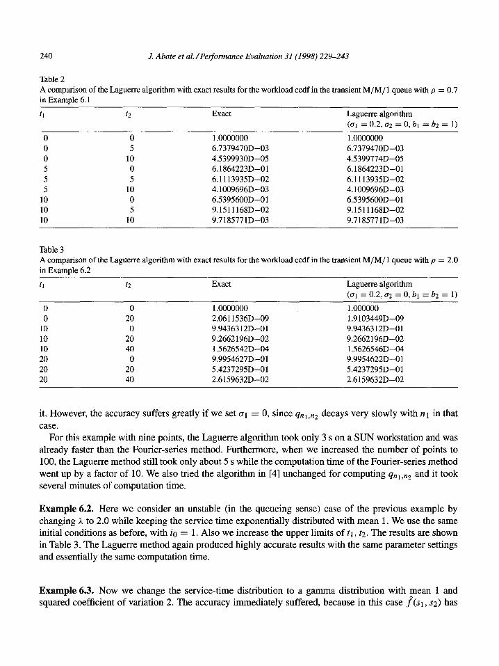
240 J. Abate et al. /Petiomzance Evaluation 31 (1998) 229-243

Table 2 A comparison of the Laguerre algorithm with exact results for the workload ccdf in the transient M/M/l queue with p = 0.7

in Example 6.1

t1 t2 Exact Laguerre algorithm (al = 0.2, a2 = 0, bl = b2 = 1)

0 0 0 5 5 5

10 10 10

0 1 .oooOOoo 1 .oOOOOOo 5 6.7379470D-03 6.737947OD-03

10 4.5399930D-05 4.5399774D-05 0 6.1864223D-01 6.1864223D-01 5 6.1113935D-02 6.1113935D-02

10 4.1009696D-03 4.1009696D-03 0 6.5395600D-01 6.53956OOD-01 5 9.1511168D-02 9.1511168D-02

10 9.7185771D-03 9.7185771D-03

Table 3 A comparison of the Laguerre algorithm with exact results for the workload ccdf in the transient M/M/ 1 queue with p = 2.0 in Example 6.2

t1

0 0

10 10 10 20 20 20

t2 Exact

0 20

0 20 40

0 20 40

1 .oOOOOOo 1 .oooooo 2.0611536D-09 1.9103449D-09 9.9436312D-01 9.9436312D-01 9.2662196D-02 9.2662196D-02 1.5626542D-04 1.5626546D-04 9.9954627D-01 9.9954622D-01 5.42372951)-01 5.4237295D-01 2.6159632D-02 2.6159632D-02

Laguerre algorithm

(at = 0.2, a2 = 0, bl = b2 = 1)

it. However, the accuracy suffers greatly if we set ~1 = 0, since qnl ,n2 decays very slowly with nt in that case.

For this example with nine points, the Laguerre algorithm took only 3 s on a SUN workstation and was already faster than the Fourier-series method. Furthermore, when we increased the number of points to 100, the Laguerre method still took only about 5 s while the computation time of the Fourier-series method went up by a factor of 10. We also tried the algorithm in [4] unchanged for computing qn,,n2 and it took several minutes of computation time.

Example 6.2. Here we consider an unstable (in the queueing sense) case of the previous example by changing h to 2.0 while keeping the service time exponentially distributed with mean 1. We use the same initial conditions as before, with iu = 1. Also we increase the upper limits of tl , t2. The results are shown in Table 3. The Laguerre method again produced highly accurate results with the same parameter settings and essentially the same computation time.

Example 6.3. Now we change the service-time distribution to a gamma distribution with mean 1 and squared coefficient of variation 2. The accuracy immediately suffered, because in this case f^(sr, ~2) has

J. Abate et al./Pelformance Evaluation 31 (1998) 229-243 241

Table 4 A comparison of the L.aguerre algorithm with exact results for the workload ccdf in the transient M/G/l queue having a gamma service-time di:stribution with mean 1 and SCV 2 and arrival rate ,c = 0.7 in Example 6.3

t1 t2 Exact Laguerre algorithm (al = 0.2, a;! = 0, bl = 1, b2 = 5)

0 0 0 5 5 5

10

10 10

0 1 .OOOOOO0DO 0 0.9696784DO

5 2.5347319D-02 2.5347463D-02

10 1.5654023D-03 1.5656101D-03

0 5.8817561D-01 5.8123322D-01

5 l.O482486D-01 l.O482486D-01

10 1.7541753D-02 1.7541750D-02 0 6.273531 lD-01 6.2729503D-01 5 1.4833812D-01 1.4833806D-01

10 3.2697995D-02 3.2697984D-02

a singularity at s2 I= -co; see [l] for a detailed explanation. To improve accuracy, we increase both Nl and N2 by factors of 2 (which increased computation time by about 5-6 times) used the epsilon algorithm in both dimensions and increased b2 to 5. All these steps improved accuracy to a level that should be satisfactory for most applications, but the final accuracy is still less than that of Example 6.1, as can be seen from Table 4.

Remark 6.1. It appears that if the transform does not have a singularity at si = -cc for i = 1 or 2, then the Laguerre method with our efficient two-dimensional FFI-based implementation would clearly be the method of choice. Ckherwise, the Fourier-series method, which is more robust, would be preferable. In case the transform is badly behaved, instead of trying to fix the Laguerre method, as we do in Example 6.3, a better approach might be to change the transform. In Example 6.3, if we replace the gamma service-time distribution by a distribution with a rational Laplace transform that matches the first several moments (e.g., the H2 distribution lean match the first three moments), then the Laguerre method would behave just as well as in Example 6.1.

7. Summary of the algorithm

As with the one-dimensional algorithm in [l, Section lo], we conclude this paper by summarizing the algorithm. We describe the FFT variant, using the enhancements described in Sections 4.14.3. Since the further refinements here parallel those in [ 11, we refer to [l, Section lo], for a summary of further refine- ments.

Basic FFT-based algorithm

Step 1: Compute and store the approximate Laguerre coeficients qnl,n2 for 0 5 nl 5 N1 - 1 and 0 5 n2 5 N2 - 1. First, for i = 1,2 specify the parameter Ni as powers of 2, e.g., Nt = N2 = 128. Then specify the roundoff-error-control parameters Zi (also as powers of 2), e.g., It = 1 and 12 = 2. Then let mi = 2ZiNi. Choose the parameters Ai to control the aliasing error in (18) and (19), e.g., Al = 11 and A2 = 13. Then let ri = lo- Ailmi for i = 1,2. Successively compute and store (bn,,n2}, {an,+*}

242 J. Abate et al./Per$ormance Evaluation 31 (1998) 229-243

and 14nl,n2 } via (23), (25)-(26) and (22), where Q(z1, ~2) is obtained from the given Laplace transform

f(sl, $2) via (5). (The FFT is used in (25)-(26).) Step 2: Compute and store the Laguerre function values l,(t) for 0 5 IZ _< max{Nl - 1, N2 - l}for

each required t. It is convenient to let the set of argument pairs (tl , t2) be a product set T x T. Then 1, (t) is needed for each t E T. For each t, the recursion (14) is used.

Step 3: Compute the desiredfunction values f (tl , t2) from (2).

Step 4: Make an accurucy check. To verify accuracy, repeat the computation with a different pair of roundoff-error-control parameters (Zl,Z2); e.g., if (II, 12) was (1,2), then repeat the calculation with (Zl,Z2) =

(272).

References

[l] J. Abate, G.L. Choudhury and W. Whitt, On the Laguerre method for numerically inverting Laplace transforms, Informs

J. Comput. 8 (1996) 413-427. [2] J. Abate and W. Whitt, Solving probability transform functional equations for numerical inversion, Opel: Res. L&t. 12

(1992) 275-281. [3] G.L. Choudhury and D.M. Lucantoni, Numerical computation of the moments of a probability distribution from its

transform, Opel: Res. 44 ( 1996) 368-38 1. [4] G.L. Choudhury, D.M. Lucantoni and W. Whitt, Multidimensional transform inversion with applications to the transient

M/G/l queue, Ann. Appl. Probab. 4 (1994) 719-740.

[5] G.L. Choudhury, D.M. Lucantoni and W. Whitt, Numerical solution of Ml/G,/1 queues, Oper. Res. 45 (1997), to appear. [6] G.L. Choudhury and W. Whitt, Computing distributions and moments in polling models by numerical transform inversion,

Performance Evaluation 25 (1996) 267-292.

[7] G.L. Choudhury and W. Whitt, Probabilistic scaling for the numerical inversion of non-probability transforms, Informs.

J. Comput. 9 (1997), to appear. [8] V.A. Ditkin and A.P. Prudnikov, Operational Calculus in Two Variables and Its Applications, 2nd ed., Academic Press,

New York ( 1962). [9] B.S. Garbow, G. Giunta, J.N. Lyness and A. Murli, Software for an implementation of Weeks’ method for the inverse

Laplace transform problem, ACM Trans. Math. Software 14 (1988) 163-170.

[lo] B.S. Garbow, G. Giunta, J.N. Lyness and A. Murli, Algorithm 662: A FORTRAN software package for numerical inversion of the Laplace transform based on Weeks’ method, ACM Trans. Math. Software 14 (1988) 171-176.

[ 1 I] M.V. Moorthy, Inversion of the multi-dimensional Laplace transform - expansion by Laguerre series, Z. Angew. Math.

Phys. 46 (1995) 793-806.

[ 121 M.V. Moorthy, Numerical inversion of two-dimensional Laplace transforms - Fourier series representation, Appl. Nume,: Math. 17 (1995) 119-127.

[ 131 A.V. Oppenheim and R.W. Schafer, Digital Signal Processing, Prentice-Hall, Englewood Cliff, NJ (1975). [ 141 W. Rudin, Real and Complex Analysis, McGraw-Hill, New York (1966). [15] U. Sumita and M. Kijima, The biva.riate Laguerre transform and its applications: Numerical exploration of bivariate

processes, Adv. in Appl. Probab. 17 (1985) 683-708.

[16] G. Szegii, Orthogonal Polynomials, 4th ed., Amer. Math. Sot. Colloq. Publ., Vol. 23, AMS, Providence, RI (1975). [17] B. Van der Pol and H. Bremmer, Operational Calculus, Cambridge University Press, Cambridge (1955) (reprinted in

1987 by Chelsea Press, New York). [ 181 W.T. Weeks, Numerical inversion of Laplace transforms using Laguerre functions, J. ACM 13 (1966) 419-426. [ 191 J. Wimp, Sequence Transformations and Their Applications, Academic Press, New York (1981). [20] I? Wynn, On a device for computing the e, (S,) transformation, Math. Tables Aids Comput. 10 (1956) 91-96. [21] P. Wynn, On the convergence and stability of the epsilon algorithm, SZAMJ. Numer: Anal. 3 (1966) 91-122.

.I. Abate et al. /Pe$omance Evaluation 31(1998) 229-243 243

Ward Whitt received the A.B. degree in Mathematics from Dartmouth College, Hanover, NH, USA, in 1964 and the Ph.D. degree in Operations Research from Cornell University, Ithaca, NY, USA, in 1969. He was on the faculty of Stanford University and Yale University before joining AT&T Laboratories in 1977. He is currently a member of the Network Mathematics Research Department in AT&T Labs- Research in Florham Park, NJ, USA. His research has focused on probability theory, queueing models, performance analysis and numerical transform inversion.

Gagan L. Choudhury received the B.Tech. degree in Radio Physics and Electronics from the Univer- sity of Calcutta, India in 1979 and the MS and Ph.D. degrees in Electrical Engineering from the State University of New York (SUNY) at Stony Brook in 1981 and 1982, respectively. Currently he is a Technical Manager at the Teletrafhc Theory and System Performance Department in AT&T Laborato- ries, Holmdel, New Jersey, USA. His main research interest is in the development of multi-dimensional numerical transform inversion algorithms and their application to the performance analysis of telecom- munication and computer systems.

Joseph Abate received the B S. degree from the City College of New York in 1961, and the Ph.D. degree in Mathematical Physics from New York University in 1967. From 1966 to 1970 he was employed by Computer Applications Corporation where he specialized in evaluating the performance of real- time computer systems. In 1971, he joined AT&T Bell Laboratories and retired in 1990. For most of his career, he worked on the design and analysis of transaction processing systems used in support of telephone company operations. For many years he has had a great passion for the use of Laplace transforms in queueing problems.

Currently, he is a contractor to Lucent Technologies in Liberty Comer, New Jersey.