Numerical experiments with the LANCELOT … · In this paper, we describe the algorithmic options...

Mathematical Programming 73 (1996) 73-110

Numerical experiments with the LANCELOT package(Release A) for large-scale nonlinear

optimization 1

A.R. Conn a, Nick Gould b, Ph.L. Toint c,, a IBM T.J, Watson Research Center, P.O. Box 218, Yorktown Heights, NY 10598, USA

b Computing and Information Systems Department. Rutherford Appleton Laborato~, Chilton, UK c Department ofMathernatics, Facultds Universitaires Notre Dame de la Paix, 61. rue de Brua'elles,

B-5000 Namur, Belgium

Received 6 October 1992; revised manuscript received 18 September 1995

Abstract

In this paper, we describe the algorithmic options of Release A of LANCELOT, a Fortran package for large-scale nonlinear optimization. We then present the results of intensive numerical tests and discuss the relative merits of the options. The experiments described involve both academic and applied problems. Finally, we propose conclusions, both specific to LANCELOT and of more general scope.

Keywords: Large-scale problems; Nonlinear optimization; Numerical algorithms

1. Introduction

Research in large-scale optimization has been, in recent years, a major subject of interest within the mathematical programming community, as is clear from the programs of the main conferences and symposia on optimization techniques during this period. One such project was initiated by the authors of this paper [12] and has resulted in both theoretical contributions and software for large nonlinear optimization problems. A

" Con-esponding author. E-mail [email protected]. This research was supported in part by the Advanced Research Projects Agency of the Department of

Defense and was monitored by the Air Force Office of Scientific Research under Contract No F49620-91-C- 0079.

0025-5610 �9 1996 - The Mathematical Programming Society, Inc. All fights reserved SSDI 0 0 2 5 - 5 6 1 0 ( 9 5 ) 0 0 0 5 4 - 2

7 4 A.R. Corm et at. / Mathematical Programming 73 (I 996) 73-110

detailed description of the algorithms developed and implemented in LANCELOT, the resulting Fortran package, is presented in [15]. The purpose of the present paper is to report on the numerical experiments performed with this software on a sizeable

collection of test problems, and to draw some first conclusions on the respective merits of the algorithmic options available in the package. A comparison of LANCELOT and

MINOS [45] is currently being conducted on a large set of test problems. However, due to the diversity of algorithmic options and complexity of these two packages, a fair and

informative comparison is, in itself, a major research effort. It will be reported on

separately. The paper is organized as follows. Section 2 briefly presents the main features and

structure of LANCELOT. Section 3 contains a general description of SBMIN, the kernel algorithm for the software that handles simple bounds. AUGLG, the component that

handles the extension to general constraints, is then outlined in Section 4. Section 5 discusses the various algorithmic options that are available within the package. Section 6 presents the testing framework and the strategy used to analyze the results. These results are then discussed in more detail in Section 7, where the efficiency and robustness of

various algorithmic options are compared. Finally, some conclusions and perspectives are drawn in Section 8.

2. General features and structure of the LANCELOT package

2.1. Package presentation

The purpose of the LANCELOT package is to solve the general nonlinear programming problem

min f ( x ) (2.1) x ~ n

subject to the constraints

c (x ) = 0, (2.2)

and to the simple bounds

l i<~x i ~ u i, i = l . . . . . n, (2.3)

where f and c are assumed to be smooth functions from ~" into [R and from IR" into Nm, respectively. The package is specially intended for problems where n a n d / o r m are large. Indeed, it exploits the (group) partially separable structure (see [12]) of most large-scale optimization problems. However, the package can also be applied successfully to small problems. The algorithms are designed to provide convergence of the

generated iterates to local minimizers from all starting points. There is no loss in assuming that all the general constraints are equality constraints,

as inequality constraints may easily be transformed to equations by the addition of extra

A.R. Corm et al./Mathematical Progratmning 73 (1996) 73-110 75

slack or surplus variables (see, for example, [31, Section 5.6]). Indeed, LANCELOT automatically transforms inequality constraints to equations. This technique is exten-

sively used in simplex-like methods for large-scale linear and nonlinear programs. General features include facilities to compute numerical derivatives, an analytical

derivative checker and an automated restart. The software also uses a full reverse

communication interface for greater flexibility and adaptability. The package is written in standard ANSI Fortran77. It has already been ported to

CRAY and IBM mainframes, to Digital VAX minicomputers, and to Digital, Hewlett- Packard, IBM, Silicon Graphics and Sun workstations, as well as to DOS-based personal computers. A fully automated installation procedure is supported for all these

machines/systems. Single and double precision versions are available. The program's dimensions are also adaptable to fit within machines with different memory sizes.

Full information on the package is available in [15]. Interested parties should contact

one of the authors.

2.2. The algorithmic structure of the package

Because the purpose of this paper is to discuss the relative merits of several algorithmic options within the package, it is necessary to provide first a general description of the numerical methods used. The structure of the LANCELOT algorithms is summarized in Fig. 1.

The package (whose algorithmic components appear in the rounded box) reads the problem as a set of data and Fortran subroutines (for computing function and derivatives

Users and problems [ . . . . . . . . . . . . . . . . . . . . . . . . . . . . . . . - [ - . . . . . . . . . . . . . . . . . . . . . . . . . . . . . . . . . . . . . . . . . . . ,'

Standard Input Format (SIF) interpreter /

l

Direct

linear

solvers

LANCELOT interface

11 AUGLG

11 SBMIN

li Iterative linear solvers

i

Preconditioners

Fig. 1. Structure of the LANCELOT package.

76 A.R. Corm et al./Mathematical Programming 73 (1996) 73-110

values, as well as other problem related tasks). The way in which these subroutines and the associated datafile are produced is not the subject of this paper. It suffices to say that they can be written directly by the user, or obtained as the result of the automated interpretation of the problem expressed in a more friendly Standard Input Format. These techniques are described in detail in [15] and will not be discussed further here. We will rather concentrate on the algorithms used by LANCELOT to solve the problem, once properly specified. As suggested by the picture, LANCELOT either uses an augmented Lagrangian approach (if constraints of the type (2.2) are present), or directly attempts to solve problems whose only constraints are simple bounds, (2.3).

The augmented Lagrangian algorithm AUGLG is outlined in Section 4. Its convergence theory has been analyzed in [13,16]. This theory guarantees that, under standard assumptions, the sequence of iterates calculated by the algorithm converges to a local minimizer of the problem. This augmented Lagrangian method proceeds by solving a sequence of suitably defined nonlinear optimization problems with simple bound constraints. We will call these iterations of the augmented Lagrangian algorithm major

iterations.

If the problem under consideration possesses only simple bounds, a specialized algorithm, S[3MIN, can be applied. This algorithm is of trust region type and is presented in Section 3. Its strong convergence properties have been analyzed in [10,38,51]. At the heart of SBMIN, quadratic problems with bound constraints (BQP) are solved repeatedly. In fact, a BQP is approximately solved at every SBMIN iteration. We call these minor iterations.

The process of (approximately) solving the BQP involves the (approximate) solution of a linear system of equations. This can be achieved by applying either direct or iterative linear solvers. The latter typically require preconditioning, which in turn might call specialized versions of the direct solvers, as is shown in the figure above. The iterative technique used with the package is preconditioned conjugate gradients. Itera- tions at this level are simply called cg-iterafions. Note that some form of preconditioning might require a very problem specific technique; hence there is the possibility to return to the user level for such a calculation.

The three nested iteration levels (major iterations at the augmented Lagrangian level, minor iterations at the SBMIN level, and cg-iterations at the BQP level) are illustrated in Fig. 2, where the dashed boxes indicate iteration levels that need not be present for all problems and all choices of algorithmic options.

. . . . . . . . . . . . . . . . . . . . . . . . . . . . . . . . . . . . . . . . . . . . .

AUGLG: m a j o r i t e ra t ions

SBMIN: minor i t e ra t ions . . . . . . . . . . . . . . . . . . . . . . . . . . . . . . . . . . . .

i i

', BQP: cg- i tera t ions ',

Fig. 2. The nested iteration levels within LANCELOT.

A.R. Connet al. / Mathematical Programming 73 (1996) 73-110 77

As the bulk of the computational work is performed in the minor and cg-iterations,

we now summarize these parts of the algorithm. The reader is urged to consult Chapter 3

of [15] for further details.

3. An outline of SBMIN

SBMIN is a method for solving the bound-constrained minimization problem defined

by (2.1) and the simple bound constraints (2.3). Here, f is assumed to be twice-continu-

ously differentiable and any of the bounds in (2.3) may be infinite. We will denote the

vector of first partial derivatives, V~f(x), by g (x ) and the Hessian matrix, Vxxf(x), will be denoted by H(x). We shall refer to the set of points which satisfy (2.3) as the

feasible box and any point lying in the feasible box is said to be feasible. SBMIN is an iterative method. At the end of the kth iteration, an estimate of the

solution, x (k), satisfying the simple bounds (2.3), is given. The purpose of the (k + 1)st

iteration is to find a feasible iterate x (k+ ~) which is a significant improvement on x (k). In the (k + 1)st iteration, we build a quadratic model of our (possibly) nonlinear

objective function, f (x ) . This model takes the form

m(*'(x) = f ( x (*)) +g(x(*))T(x--x (k)) +�89 (3.1)

where B (*) is a symmetric approximation to the Hessian matrix H(x(k)). We also define a scalar _4 (*), the trust-region radius, which defines the trust region,

II x - x <*> [I -<< ~ ( * ) , (3.2)

within which we trust that the values of m(k)(x) and f(x) will generally agree sufficiently. An appropriate range of values for the trust-region radius is accumulated as the minimization proceeds.

The (k + 1)st iteration proceeds in a number of stages. These may be summarized, in order, as follows.

(1) Test for convergence. The calculation is stopped when the projected gradient is small enough, that is when

II x<k) -- P ( x<k> -- g ( x(*>), Z, u) l[= < E~

for some appropriate small convergence tolerance e~, where

P( x, l, u)i= man(max(l/, xi), ui).

holds

(3.3)

(3.4)

(2) Find the generalized Cauchy point of the quadratic model (see Section 3.1). (3) Obtain a new point which further reduces the quadratic model within the

intersection of the feasible box and the trust region (see Section 3.2). (4) Test whether there is a general agreement between the values of the model and

true objective function at the new point. If so, accept the new point as the next iterate (the iteration is then said to be successful). Otherwise, retain the existing iterate as the

78 A.R. Corm et al. / Mathematical Pro~,,ramming 73 (1996~ 73-110

next iterate (the iteration is unsuccess2tid). In either case, adjust the trust region radius as appropriate (see Section 3.2.4 of [15]).

3.1. The generalized Cauchy point

The approximate minimization of the quadratic model (3.1) within the intersection of

the feasible box and the trust region at the (k + 1)st iteration is accomplished in two

stages. In the first, we obtain the so-called generalieoed Cauchy point (GCP), which is

the result of this minimization carried out only on the path defined by the projection of

the model 's negative gradient onto this intersection. This point is important mostly

because convergence of the algomhm to a point at which the projected gradient is zero

can be guaranteed provided the value of the quadratic model at the end of each minor

iteration is no larger than that at the generalized Cauchy point (see [10]).

An efficient algorithm for this calculation, ,,,,'hen the trust region is defined in the

infinity-norm (the LANCELOT default), is given in [11]. However, it is not necessary

that the generalized Cauchy point be calculated exactly. Indeed, a number of authors

have considered approximations which are sufficient to guarantee convergence (see

[6-8,40,51]). Consequently we provide the option of using the approximation suggested by Mo,d in [40]. Since in our experience this option has proved to be less reliable and

less efficient than the exact calculation, we will not discuss it further. Interested readers are referred to [15].

3.2. Beyond the generalized Cauchy point

We have ensured that SBMIN will converge by determining the generalized Cauchy

point. Convergence at a reasonable rate is achieved by, if necessary, further reducing the quadratic model.

Those variables which lie on their bounds at the generalized Cauchy point are fixed. Attempts are then made to reduce the quadratic model by changing the values of the

remaining free variables. Let x Ik'j) be the obtained generalized Cauchy point and let x (k'i~, j = 2, 3 . . . . . be distinct points such that:

�9 x (~'.i) lies within the intersection of the feasible box and the trust region;

�9 those variables which lie on a bound at x (k'~) lie on the same bound at x(k'.i); �9 x tkj+ ~) is constructed from x (k-i) by

(1) determining a nonzero search direction p(k.i) for which

E c*,r (3.5) m" ~, .'r(e'jl) T p (k'j) < 0:,

(2) finding a steplength o?kJ)> 0 which minimizes m(~)(.r (~ J)+ c~p (k'j)) w i t h i n

the intersection of the feasible box and the trust region; and (3) setting

x (~'j+ ~) = .r (k'i) + c~(k'-J~p {k4). (3.6)


This process is stopped when the norm of the free gradient of the model at x (t'J) is sufficiently small. The free gradient of the model is

O(V,m'~)(x(~J)) , x (.4), l, u), (3.7)

where the operator

{y~, if I i < x i < u i, Q( y, x, l, u)i = 0, otherwise,

(3

zeros components of the gradient corresponding to variables which lie on their bounds. In LANCELOT, we stop when

[10(V~m(*)(x(*'J)), x (*'J), l, u)l[ ~< 11Q(V,m(*)(x(*)), x (*''), l, u)[1 t . s (3.9)

which is known (see [38]) to guarantee that the convergence rate of the method is asymptotically superlinear.

There is much flexibility in obtaining a search direction which satisfies (3.5). We determine such a direction by finding an approximation to the minimizer of the

quadratic subproblem (3.1), where certain of the variables are fixed on their bounds but the constraints on the remaining variables are ignored. Specifically, let ,.:(*'J) be a set

of indices of the variables which are to be fixed, let e~ be the ith column of the n by n identify matrix 1 and let i (*'j) be the matrix made up of columns er i f f d r Now define

~(k,:)_ i(k4)Vg(k.j) and ~k,j) = i(k.j)'rB(k.j)i(k.i)" (3.10)

Then the quadratic model (3.1) at x (k'j) + p , considered as a function of the free variables ~ = i(k':)'rp, is

i ~ 'r~(k.j~ (3.1 1 ) = x + + ,. ,..

We may attempt to minimize (3.11) using either a direct or iterative method. In a direct minimization of (3.11), one factorizes the coefficient matrix ~(k,j). If the

factors indicate that the matrix is positive definite, the Newton equations

B(~'J)~*'J) = - ~(*'J) (3.12)

may be solved and the required search direction p(* 'J)= ~(*.J)fi(k.D recovered. If, on the other hand, the matrix is merely positive semi-definite, a direction of linear infinite descent or a weak solution to the Newton equations can be determined. Finally, if the matrix is truly indefinite, a direction of negative curvature may be obtained.

In an iterative minimization of (3.11), the index set J:(k'J) may stay constant over a number of iterations, while at each iteration the search direction may be calculated from the current model gradient and Hessian B(*'J) and previous search directions. The iterative method used in LANGELOT is the method of conjugate gradients. The convergence of such a method may be accelerated by preconditioning (see below). In fact the boundary between a good preconditioned iterative method and a direct method is quite blurred.

80 A.R. Corm et a l . / Mathematical Programming 73 (1996) 73-110

4. An outline of AUGLG

AUGLG is a method for solving the generally-constrained minimization problem defined by (2.1)-(2.3). As above, f and the cj are all assumed to be twice-continuously differentiable and any of the bounds in (2.3) may be infinite.

The objective function and general constraints are combined into the augmented Lagrangian

IFI 1 Irtl

4 ( x, A, S, /x) = f ( x ) + i=, y" Aici(x) + 2--~i~=l siici( x)2, (4.1)

where the components A s of the vector A are known as Lagrange multiplier estimates, the entries sii of the diagonal matrix S are positive scaling factors, and /x is known as the penalty parameter.

The constrained minimization problem (2.1)-(2.3) is now solved by finding approximate minimizers of �9 subject to the simple bounds (2.3), for a carefully constructed sequence of Lagrange multiplier estimates, constraint scaling factors and penalty parameters.

The (k + 1)st major iteration of AUGLG is made up of three steps. At the start of the iteration, Lagrange multiplier estimates, A (k~, constraint scaling factors, S (k), and a penalty parameter/x (~) are given. The steps performed may be summarized, in order, as follows.

(1) Test for convergence. The calculation is stopped when the projected Lagrangian gradient and the constraint violation are both small enough, that is when

IIx~)-P(x ~ - VxL(" x~, A ~>), l, u)ll= ~ ~, and [[c(xCk~)ll=<,c (4.2)

hold for some appropriate small convergence tolerances e t and eL. (2) Use SBMIN to find an approximate minimizer, x (k+I), of the augmented

Lagrangian function ~ ( x , A (k), S (~), /z ~)) in the feasible box, (2.3). This approximate minimization is terminated when

II x ~+ ~) - P ( x ~+ .7 _ V,~( x<~+ ,), ,X(~), S(~, ~z~k)), 1, u)II-<< w <k) (4.3)

is satisfied for some tolerance w ~k). (3) Update the Lagrange multiplier estimates or the penalty parameter, depending on

the value of II c(x ~§ ~)11, in addition to convergence and feasibility tolerances and constraint scaling factors (see Section 3.4.3 of [15]).

5. Algorithmic options within LANCELOT

We now discuss the most successful algorithmic options available in LANCELOT. We refer the reader to [15] for a comprehensive description of all options, and to [18] for exhaustive numerical results.

A.R. Conn et al. / Mathematical Programming 73 (1996) 73- I 10 81

5.1. Constraint and variable scaling

LANCELOT allows the user to specify variable and constraint scalings as input parameters and the scalings are then used implicitly by the algorithms. It is also possible to construct automatic scalings independent of the minimization routines by applying the matrix equilibration algorithm of Curtis and Reid [20] to the matrix formed by augmenting the constraint Jacobian with the objective function gradient. The resulting scale factors may then be used as scalings for the nonlinear problem (see Section 3.5 of [15]). Specifically, LANCELOT uses the implementation given by MC29 in the Harwell Subroutine Library. This automatic scaling procedure is available as an option within LANCELOT and will be referred to as the "scaling" option. Note that the stopping criteria (3.3) and (4.2) are suitably adapted to reflect scaling when this option is invoked.

5.2. Linear solvers

Most of the LANCELOT algorithmic options are related to the way in which an (approximate) minimizer of (3.11) is computed. This is hardly surprising since one expects the burden of the numerical calculation to be at this level.

5.2.1. Direct methods Once the set d ~ ' ( k ' j ) is determined, the nature of the quadratic model restricted to the

subset of free variables is characterized by the inertia of the matrix B(*'J). If all the eigenvalues of B(*'J) are strictly positive, the unique minimizer of (3.11) is given as the solution to the Newton equations (3.12). In all other cases, the model (3.11) is either singular or unbounded below.

The use of a sparse multifrontal direct method to solve large-scale optimization problems has been advocated in [9]. Briefly, the matrix ~(k,j) is factorized using the Harwell Subroutine Library code MA27 [26,27] as

~(k,j) = ~ (*../~Z(k.j)~(,.j)~(,.j)T- n (k.j)r, (5.1)

where ~(k,j) is a permutation matrix, L(*'J) is unit lower triangular and D(~'J) is block-diagonal with 1 x 1 and 2 X 2 diagonal blocks. The inertia of ~(k.j) and ~(*.J) are identical.

An option within LANCELOT, denoted by the "seml t f " symbol, has the key property that the Newton direction is always chosen if ~(k.j) is positive definite and is based on the modified Cholesky methods of Schnabel and Eskow [49]. Here, we form a factorization

~(k , j ) ..[_ F_(k.j) = 7_Jk,j)~(k,j)~(k,j)T, (5.2)

where Z (k'-~) is unit lower triangular, ~(k,j) is positive definite and diagonal, and ~(k,i) is positive semi-definite, diagonal and nonzero only when ~(,.j) is not (sufficiently) positive definite. It is straightforward to modify the Harwell subroutine MA27 to

8 2 A.R. Corm et al. / Mathematical Programming 73 (1996) 73-110

achieve this factorization. Now, the modified Newton equations

(~(k , j ) + fx~,j~) ~(~,j) = _ ~,(k.j) (5 .3 )

are solved to obtain a suitable search direction. More than one cycle of improvement beyond the Cauchy point is allowed with this option.

We stress that an advantage of this technique is that B (k) will typically not be modified as we approach the solution to the problem. Moreover, provided the trust-re-

gion radius is sufficiently large that the Newton step (3.12) may be taken, we would also

expect to take very few inner-iterations (indeed, in the nondegenerate case, one) before

(3.9) is satisfied. Another option of the package, based on factorizing B(*J) instead of ~(k.j) + F(k,j),

is discussed in [9]. Its performance is generally inferior to that of semN.

5.2.2. Iterative methods In LANCELOT, the iterative method of choice is the method of conjugate gradients

(see, for example, [31, Section 4.8.3] or [32, Sections 10.2 and 10.3]). Such a method attempts to find a stationary point of a quadratic function, in our case (3.11), by generating a sequence of (conjugate) search directions, ~(k4). If ~(k4) is not positive definite, the sequence of conjugate gradients may terminate with a direction along which the model (3.11) is either constant or unbounded below.

The convergence of the conjugate gradient method may be enhanced by preconditioning the coefficient matrix ~(k.j). A preconditioner is a symmetric, positive definite matrix P(~'J) which is chosen to make the eigenvalues of the product F (k'j)- ~(k,j) cluster around as few distinct values as possible. We have tried to supply a representa- tive cross-section of widely used preconditioners. We recognize that users may have a better idea of a good preconditioner for their problem by allowing them to provide their o w n ,

Band preconditioners. Many application areas give rise to problems whose Hessian matrices are banded. A band matrix is a matrix B for which bij = 0 for all [i - - j [ > mb. The smallest integer m b for which this is so is known as the semi-bandwidth of the matrix. The significant property as far as we are concerned is that, if B is positive definite, the Cholesky factors fit within the band. Moreover, clever storage schemes have been constructed to make the factorization and subsequent solutions extremely efficient (see, for example, [25, Section 10.2] and [29, Chapter 4]). We offer a band preconditioner within LANCELOT. This works in two stages. The desired semi-bandwidth, m b, is assumed to have been specified. The band matrix ~(k.j), with semi-bandwidth m b, is chosen so that

M.[['J) = B~'-/), for all [i - l] ~< m,,. (5.4)

Then, we obtain a modified Cholesky factorization of ~}k.j), as described in Section 5.2.1.

When ~(k..0 is positive definite and rn b is chosen large enough, the preconditioned conjugate gradient method will converge in a single iteration. The effect of the

A.R. Corm e t a I. / M a t h e m a t i c a l P r o g r a m m i n g 73 (1996) 73 ~ 110 83

preconditioner in other cases has not been formally analyzed. Band preconditioners are denoted below by "ban0(mb)" .

Incomplete factorization preconditioners. It is sometimes possible to construct good preconditioners for specially structured problems by either rejecting all fill-in during the factorization or by tolerating a modest amount. Such incomplete factorization

preconditioners are very popular with researchers in partial differential equations and it is possible to get off-the-shelf software to form them. We include in LANCELOT the

example MA31, due to Munksgaard [44], from the Harwell Subroutine Library. We denote this option by " m u n k s g " .

Full-matrix preconditioners. Finally, as we alluded to in Section 5.2.2, if space permits and ~(k,j) is positive definite, one can always use a complete factorization of

~(k,j) as a preconditioner. However, if ~k,j) is not positive definite, it is possible to use

the modification (5.2) suggested in Section 5.2.1 to determine a preconditioner. We consider two possible ways to obtain the perturbation matrix ~(k.j) in (5.2). The

first is, as above, the modified factofization algorithm proposed by Schnabel and Eskow in [49]. We will use " s e p r c " to denote this strategy.

It is worthwhile noting the parallel between seprc and semltf. They both use the direct modified factorization of B(*'J) to compute the Newton direction in the subspace of free variables. They differ in that this process is stopped in seprc as soon as the only bounds encountered are trust region bounds, while the minimization may be pursued, in semltf, along the trust region boundaries.

The second is another modification of MA27 advocated by Gill, Murray, Poncel~on and Saunders in [30]. Here, the factorization (5.1) is not modified as it is formed, but it is instead computed and then modified. The resulting algorithmic option is denoted below by "gmpsprc".

Expanding Band Preconditioners. One further possibility is to use an expanding band preconditioner. Consider the band matrix M!k'J~ given by (5.4), where the semi-bandwidth m b is given by

n, i f [ l x (* l -P(x (*~-g(x*) , l , u ) [ l<~lO-2 , nl(b k ) = I 7n , if lO -~" < II x ~> - P ( x ~ - g ( x ~ ) , l, u)II .< I 0 - ' , ( 5 . 5 )

~ n, otherwise.

The idea is to select the semi-bandwidth rn(b k) at each iteration to reflect the speed and accuracy which one wants from the preconditioned conjugate gradient method. In particular, if low accuracy is required, a preconditioner with a small semi-bandwidth (such as a diagonal preconditioner) is often very effective. But if high accuracy is desired, it may be better to pick a preconditioner which is a better approximation to ~ ( k , j ) .

Having obtained the preconditioner, we obtain a modified Cholesky factorization of M[['J), as described in Section 5.2.1. However, unlike the band preconditioners described above, the matrix and its factorization are stored as a general sparse, rather than band, matrix.

84 A.R. Corm et al. / Mathematical Programming 73 (1996) 73-1 l O

We realize that further sophistication may be desirable but have found that this simple scheme is effective in practice. This preconditioning option will be denoted by "expband".

5.3. Derivative approximations

Further algorithmic options in LANCELOT are related to the various ways in which derivatives or their approximations are computed. However, the structure of these

derivatives crucially depends on the structure of the nonlinear functions themselves. In

order to derive an efficient algorithm for large-scale calculations, we first need to know a way to handle the structure typically inherent in functions of many variables.

A function f ( x ) is said to be group partially separable if: (1) the function can be expressed in the form

ng

f ( x ) = Y',gi(c~i(x)), where a i ( x ) = • w i j ~ ( x U]) + a m x - b i (5.6) i= t j e J ,

(%(x) is known as the ith group); (2) each of the group functions gi(c~) is a twice continuously differentiable function

of the single variable a ; (3) each of the index sets ,.el is a subset of {1 . . . . . n,.}, where n c is the number of

nonlinear element functions; (4) each of the nonlinear element functions fj is a twice continuously differentiable

function of a subset x [j] of the variables x. Each function is assumed to have a large invariant subspace. Usually, this is manifested by x IA comprising a small fraction of the

variables x. This structure is extremely general. Indeed, any function with a continuous, sparse

Hessian matrix may be written in this form (see [34]). A more thorough introduction to group partial separability is given in [12]. LANCELOT assumes that the objective function f ( x ) is of this form. When equality constraints are present, they are handled via the augmented Lagrangian and thus become part of the objective function for the subproblem given to SBMIN. Each such constraint then gives rise to the group function c~2/2/x, which imposes the restriction that each equality constraint has only a single

group. One of the main advantages of the group partially separable structure is that it

considerably simplifies the calculation of derivatives of f (x ) . If we consider (5.6), we see that we merely need to supply derivatives of the nonlinear element and group functions. LANCELOT then assembles the required gradient and, possibly, Hessian matrix of f from this information.

The gradient of (5.6) is given by

V~f(x) = E g',(%(x))V~%(x), i = l

where g~ o~,(x) = [11 wi , jEh( x ) + a , . J~'~i

(5.7)

A.R. Con,1 et al. / Mathematical Programmirlg 73 (1996) 73-110 85

Similarly, the Hessian matrix of the same function is given by

r,.~f(x) = E g"(~ r,-~ (~7, ee,(x)) T+ E g:(oe,(x))V,.,.cx~(x), i = 1 i = l

where the Hessian matrix of the ith group is

= E w,.Z,JA xlJl). j ~ ,5"-,

(5.8)

(5.9)

Notice that the Hessian matrix is the sum of two different types of terms. The first ~s

a sum of rank-one terms involving only first derivatives of the nonlinear element functions. The second involves second derivatives of the nonlinear elements. LANCELOT assumes that the first and second derivatives of the group functions are available. This is frequently the case in practice.

The quadratic model (3.1) uses the gradient of f by default. However, LANCELOT provides an option (which we will denote by " f d g " ) with which this gradient is evaluated by finite differences (see Section 3.3.2.3 of [15]). LANCELOT also offers two choices for the Hessian matrix of (3.1).

�9 We can calculate the true first and second derivatives of each nonlinear element and group function and use the exact Hessian B (~) = 77, ,f( x(~)).

�9 We can calculate the true first and second derivatives of each group function, calculate the first derivatives of the nonlinear elements but use approximations,

BI jt(~), to their second derivatives. We then use the approximation

B'k' = E g': (oei(x(k))) V~c~i(.x-ok)) (V,.c~,(x(k')) T i=i

ng

+ E g',(o,,(x",))8?', i = I

(5.1o)

where B} ~) satisfies

B} k)= Y', wi.jB[J](k) (5.11) j ~ J ,

for some suitable matrices B t4~k).

We strongly recommend the use of exact second derivatives whenever they are available. LANCELOT fully exploits this information. In our experience, because of the advantages of using partial separability, exact second derivatives are often available by direct calculation. Alternatively, one may use automatic differentiation tools (see [24,33], for instance). Using exact second derivatives is therefore the default option in the package.

However, it may sometimes be useful to approximate the matrices (5.11 ). LANCELOT presently uses the same type of derivative approximation for all elements. The symmet- tic-rank-one (SR1), Broyden-Fletcher-Goldfarb-Shanno (BFGS), Powell-symmetric- Broyden (PSB) and Davidon-Fletcher-Powell (DFP) updates are provided. We present

here the results of the first two choices, which are referred to as the " s t 1 " and " b f g s "

86 A.R. Corm et al. / Mathematical Programming 73 (1996 ~ 73-110

options respectively, since overall they were the most satisfactory. See [23,28,31] for further details on these updating formulae, ,and Section 3.3.2.3 of [15] for a more

detailed discussion of how these updates are implemented.

5.4. Accurate solution of the BQP

Finally, the last option considered in this paper allows the user to specify that the

minimization of the objective function model has to be accurate within the intersection

of the feasible region for the bound constraints and the trust region. In Section 3.2, we

gave a general framework for obtaining a new iterate that is "be t te r" than the

generalized Cauchy point. At each stage, an approximation to the minimizer of the

model is sought while some of the variables are held fixed at bounds. This set of fixed

variables, S (k'J), always includes those which were fixed at the generalized Cauchy

point. In SBM/N, we also include by default all variables which encounter bounds at

x (k'J), for j > 0 until the test (3.9) is satisfied. Then, optionally, we may free all variables

except those which were fixed at the generalized Cauchy point and perform one or more

further cycles. This optional process, denoted by " a c c b q p " , is terminated when

releasing variables does not improve the model value. This is detected when (3.9) and

l, x " J'), x l, ,,)

are satisfied. At the start of each cycle, we also compute a new generalized Cauchy point for the model fixing the variables which were on a bound at the original Cauchy

point. This recursive use of SBMIN is guaranteed to satisfy (3.9) if a sufficient number of cycles is performed.

6. The numerical tests: f r amework and p rocedure

6.1. Basic approach

There are many ways to test a complicated, general purpose code like LANCELOT, and even more ways to present the results of these tests. We now briefly discuss the

fundamental choices we made when designing our tests and which influence our

treatment of the results in this paper. Our first decision was to test and report on a large number of test cases. In our

experience, this is essential for a true assessment of reliability and performance, as smaller test sets are more likely to introduce unwanted bias.

Our second choice was to limit the comparison to reliability and efficiency aspects.

Other potential criteria, such as ease of use, accuracy of solutions and availability, did

not seem to be as significant when testing a single package.

Our final decision was to present both aggregate and relatively disaggregate perfor-

mance measures. Specifically, we chose the average performance as our aggregate measure but also report on the ranking of the algorithmic variants in five performance

A.R. CoJm et al./Mathematical Programming 73 (1996) 73-110 87

classes (excellent, good, satisfactory, fair and poor). The performance was averaged

across many problems which differ, sometimes substantially, in size, nonlinearity or type

of constraints.

Although the choice of the average sometimes obscures the performance of algorith-

mic variants on the easier problems in comparison with the harder ones, it nevertheless

seems to correspond to our intuitive appraisal of the variants after our experience of

running extensive tests. This is especially true when one also considers the associated

rankings, as we hope is apparent later in this section. Furthermore, there is little

agreement within the optimization community on alternative aggregate measures.

The authors of course realize that this scheme is not the only one that can be

defended. It is however hoped that it provides a sufficient basis to make the testing

discussed in this section of interest.

6.2. The test problems

The numerical tests with LANCELOT that we are about to describe were conducted

using the Constrained and Unconstrained Testing Environment (CUTE) collection of

nonlinear test problems (see [4]). This collection contains a large number of nonlinear

optimization problems of various sizes and difficulty, representing both academic and

real world applications. As the title of the collection implies, constrained and uncon-

strained examples are included. For our tests, we have used 624 instances of uncon-

strained (or bound constrained) problems and 319 instances of constrained problems.

These 943 instances are derived from 398 different problems, the additional examples

being determined by varying the dimension. It is of course undesirable to describe all

these examples in the present paper. It will suffice to say that our test set covers, amongst others,

�9 the "Argonne test set" [42], the Testpack report [5], the Hock and Schittkowski

collection [36], the Dembo network problems (see [21]), the Mor~-Toraldo

quadratic problems [43], the Toint-Tuyttens network model problems [52], �9 most problems from the PSPMIN collection [50], 2

�9 problems inspired by the orthogonal regression report by Gulliksson [35],

�9 some problems from the Minpack-2 test problem collection 3 [2,3] and from the second Schittkowski collection [47],

�9 a number of original problems from various application areas. We present some of the problems characteristics in Figs. 3 and 4 and in Table 1.

�9 Fig. 3 shows the distribution of the problems' dimensions.

�9 Fig. 4 illustrates the distribution of the ratio m / n , where m is the total number of general equality and inequality constraints. The higher this ratio, the more

constrained the problem. Only constrained problems (m > 0) are considered in this statistic.

2 Some trivial problems were skipped and also problems for which different local minima were known. 3 The problems that we could reconstruct from the data given in the report.

88 A.R. Corm et a l . / Mathematical Programming 73 (1996) 73-110

(5000,100001

(1(

(5oo, 1 ooo]

(48.7%)

(100,50C

(50,100] (11.9% I

Fig. 3. Distribution of problem dimensions.

�9 Table 1 reports the number of p rob lems for which a g iven character is t ic l ies in one

of five possible intervals [0, 0.2], (0.2, 0.4], (0.4, 0.6], (0.6, 0.8] and (0.8, 0.1].

Four character is t ics are examined. These are

- the relatiue nonlinearity of the objectiue fimction, that is the ratio

def number of nonl inear groups in the objec t ive

U~ -- -- number of groups in the objec t ive ' (6 .1 )

140

120 ~ . . . . . . . . . . . ~ . . . . . . . . . . . . . . . . . . . . . . . . . . . .

100 . . . . . . . . . . .

"~ 80 . . . . . . . . . . . Q..

"6 60 . . . . . . . . . . .

E

40 . . . . . . ~ - -

20 4 . . . . .

0-0.2 0.4-0.6 0.8-1.0 5.0-10.0 0,2-0.4 0.6-0.8 1.0-5.0

relative number of constra ints

Fig. 4. Distribution of tile relative number of constraints m / n.

>10.0

A.R. Conn et al. / Mathematical Programming 73 ( 1996 ) 73- l 10

Table 1 Further problems characteristics

89

~oj 48 0 13 2 880

~ons 139 5 20 8 193 n b / n 573 25 38 14 293 Y 99 5 7 13 241

where the groups are defined in (5.6) and where a group is declared nonlinear if

it contains at least one nontrivial nonlinear element function or if its associated

group function is nonlinear;

- the relative nonlinearity of the constraints, i.e.,

def number of nonlinear constraints

~'con~ = number of constraints ' (6.2)

where the bounds have been excluded from the denominator;

- the proportion n J n variables subject to bound constraints;

- the proportion of equality constraints, that is of the ratio

def number of equality constraints Y = (6.3)

m

We note the following points.

�9 The majority of the problems are not very large. However, we recall that testing

LANCELOT on small problems is meaningful because the package is also

intended to solve small-scale problems. Furthermore, the classes of larger problems are far from empty, and we note the presence of examples with more than

15 000 variables. �9 Most large problems tend to have a somewhat regular structure. As a result, most

groups in these problems tend to be structurally similar. This is noticeable in the

distribution of the relative nonlinearity of the objective function and constraints,

where either most or very few, if any, groups are nonlinear. The same phe- nomenon is also observed for the proportion of bounded variables which tends to

be either very low or close to one. �9 There are very few problems involving considerably more general constraints than

variables. Many of the problems arise as nonlinear systems of equations, while a

fair proportion have approximately half as many constraints as variables. We nevertheless note the presence of problems where the number of constraints is

substantially greater than n.

Bearing in mind that one of the LANGELOT's features is its ability to handle large problems, we also selected, amongst the 943 tests problems, all problems in more than

500 variables. This subset contains 268 problems, that is 28.1% of the complete set. The

algorithmic conclusions corresponding to the complete problem set and the subset are

90 A.R. Connet al. / Mathematical Programming 73 ('1996) 73-110

BEGIN

check-derivatives

ignore-derivative-bugs

exact-second-derivatives-used

bandsolver-preconditioned-cg-solver-used 5

exact-cauchy-point-required

trust-region-radius 1.0D+O

maximum-number-of-iterations i000

print-level -i

start-printing-at-iteration 0

stop-print•177 1000

END

Fig. 5. The LANCELOT default specification file.

interesting to compare because only the latter depends more obviously on the way in

which the problem structure is handled.

6.3. The testing procedure

Before detailing the testing procedure, we recall tile default algorithmic choice for

LANCELOT: �9 no variable/constraint scaling,

�9 a conjugate gradient linear solver is used with a banded preconditioner of semi-bandwidth 5 (band(5)),

�9 analytical second derivatives are used, as well as analytical gradients,

�9 an exact Cauchy point calculation is used, �9 the f,~-nonn is used for defining the trust region.

For our tests we also set the maximum number of iterations to 1000, the maximum cpu-time to 18000 s, the initial trust region radius to 1.0 and disabled all printing. The

accuracy requirements were set to the LANCELOT defaults, that is e t = E~ = 10 -5. We also turned the derivative checker on but chose to ignore its warning messages. Of

course, all derivatives were checked before the actual tests. For the sake of complete- ness, the default LANCELOT specification file is given in Fig. 5.

We next considered basic variants of this default choice, that is a choice of algorithmic options that differs in just one instance from the default. The basic variants are ;

noprc: no preconditioner is used within the conjugate gradient solver, i.e., ~(k.y)= I (see Section 5.2.2),

band(0): a diagonal preconditioner is used for the conjugate gradient solver (see Section

5.2.2),

A.R. Corm et ul. / Mathematical Programming 73 (1996) 73 - 110 91

band(l): a tridiagonal preconditioner is used for the conjugate gradient solver (see

Section 5.2.2), band(10): a 21-diagonals preconditioner is used for the conjugate gradient solver (see

Section 5.2.2),

expband: an expanding band preconditioner is used for the conjugate gradient solver (see Section 5.2.2),

munksg: an incomplete factorization preconditioner is used for the conjugate gradient solver (see Section 5.2.2),

seprc: a full matrix preconditioner using the Schnabel-Eskow modified factorization is

used for the conjugate gradient solver (see Section 5.2.2), grnpsprc: a full matrix preconditioner using the Gill-Murray-Poneel6on-Saunders

modified factorization is used for the conjugate gradient solver (see Section 5.2.2),

semltf: a modified multifrontal direct linear solver is used (see Section 5.2.1), st1: the symmetric-rank-one quasi-Newton formula is used to approximate second derivatives (see Section 5.3),

bfgs: the Broyden-Fletcher-Goldfarb-Shanno quasi-Newton formula is used to approximate second derivatives (see Section 5.3),

scaling: automatic variable/constraint scaling is used, with scalings computed at the starting point (see Section 5.1),

accbqp: an accurate solution to the BQP is sought (see Section 5.4).

To this list we added the fdg variant which uses finite difference approximation to gradients and the symmetric-rank-one quasi-Newton formula for approximating second derivatives (see Section 5.3). These variants and the default gives a list of 15 different algorithmic choices.

Note that the variants scaling, semltf, expband, seprc, gmpsprc and munksg depend on code from the Harwell Subroutine Library. Their use is therefore only possible for users with a suitable licence. As a consequence, they could not be selected as defaults for the package.

We then tested all of these fifteen choices on the complete problem set, which amounted to running 15 • 943 = 14 145 test cases. A total of 5658 additional cases were also run to evaluate the less successful options not discussed in this paper. These tests were performed on two Digital DECstations 5000/200 with 48 MBytes of memory, using the Ultrix f-/7 compiler (version 3.0-2) without optimization. 4 The CPU-times on both machines were checked for consistency.

7. The numerical tests: results and discussion

It is of course impossible to detail the complete set of results obtained on nearly fifteen thousand test cases in a journal article. We will therefore present and discuss

4 An error in the Fortran optimizer of this version prevented its use with the package.

92 A.R. Connet al./ Mathematical Programming 73 (1996) 73-110

summaries and averages extracted f rom these results. A technical report conta ining the

comple te results is h o w e v e r avai lable [18].

7.1. Reliabil i ty

7.1.1. General assessment

We first present results on the reliabil i ty and failures on the f i f teen a lgor i thmic

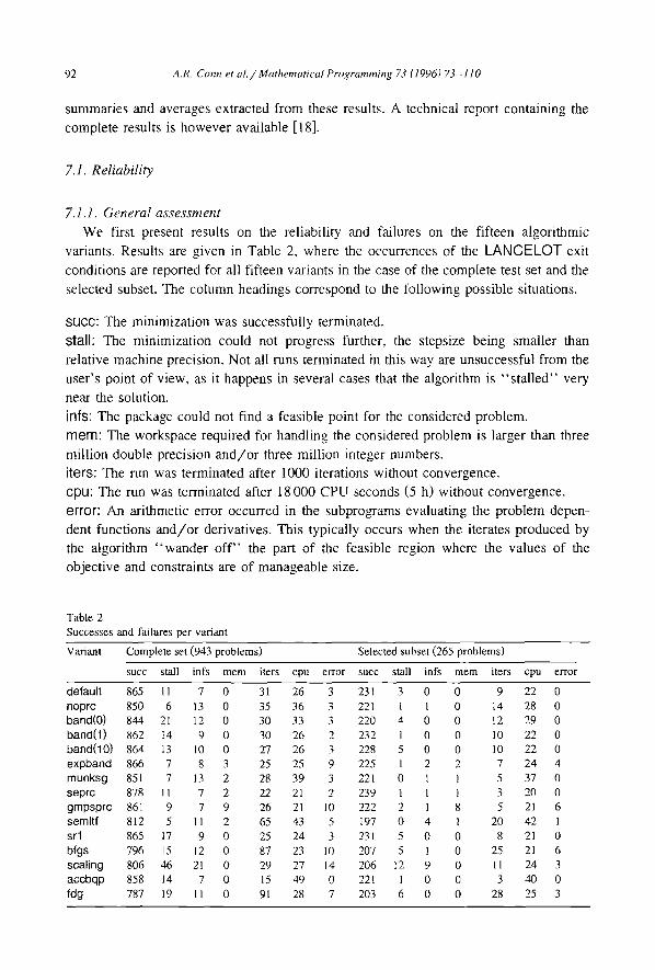
variants. Results are g iven in Table 2, where the occurrences o f the L A N C E L O T exit

condi t ions are reported for all f if teen variants in the case o f the comple te test set and the

selected subset. The co lumn headings correspond to the fo l lowing possible situations.

SUCC: The min imiza t ion was successful ly terminated.

stall: The min imiza t ion could not progress further, the stepsize being smal ler than

relat ive machine precision. Not all runs terminated in this way are unsuccessful f rom the

user ' s point o f v iew, as it happens in several cases that the a lgor i thm is " s t a l l e d " very

near the solution.

irlfs: The package could not find a feasible point for the considered problem.

m e r e : The workspace required for handl ing the considered problem is larger than three

mil l ion double precision a n d / o r three mil l ion integer numbers.

i ters: The run was terminated after 1000 iterations without convergence .

cpu : The run was terminated after 18 000 C P U seconds (5 h) wi thout convergence .

e r ror : An ari thmetic error occurred in the s u b p r o g a m s evaluat ing the p rob lem depen-

dent funct ions a n d / o r der ivat ives . This typically occurs when the iterates produced by

the algori thm " w a n d e r o f f " the part o f the feasible region where the values o f the

objec t ive and constraints are of manageab le size.

Table 2 Successes and failures per variant

Variant Complete set (943 problems) Selected subset (265 problems)

succ stall infs mere iters cpu error succ stall infs mem iters cpu error

default 865 11 7 0 3l 26 3 231 3 0 0 9 22 0 noprc 850 6 13 0 35 36 3 221 l 1 0 14 28 0 band(O) 844 21 12 0 30 33 3 220 4 0 0 12 29 0 band(l) 862 14 9 0 30 26 2 232 1 0 0 l0 22 0 band(10) 864 13 I0 0 27 26 3 228 5 0 0 10 22 0 expband 866 7 8 3 25 25 9 225 1 2 2 7 24 4 munksg 851 7 13 2 28 39 3 221 0 1 1 5 37 0 seprc 878 11 7 2 22 21 2 239 1 1 1 3 20 0 gmpsprc 861 9 7 9 26 21 10 222 2 1 8 5 21 6 semltf 812 5 II 2 65 43 5 197 0 4 1 20 42 1 srl 865 17 9 0 25 24 3 231 5 0 0 8 21 0 bfgs 796 15 12 0 87 23 I0 207 5 1 0 25 21 6 scaling 806 46 21 0 29 27 14 206 12 9 0 11 24 3 accbqp 858 14 7 0 15 49 0 221 1 0 0 3 40 0 fdg 787 19 11 0 91 28 7 203 6 0 0 28 25 3

A.R. Corm et al. / Mathematical Programming 73 (1996) 73-110 93

Note that the algorithmic variants have been ordered, in this table and subsequent figures, to allow for an easy comparison of all preconditioned iterative techniques

(themselves ordered by increasing semi-bandwidth, from noprc to gmpsprc) and of these techniques with a direct method (semltf). The default variant has been isolated for easier reference. The two quasi-Newton variants (sr] and bfgs) are then presented next

to each other, followed by the more disparate options (scaling, accbqp and fdg). From this table, we can draw the following conclusions.

(1) The reliability of the default algorithmic choice is good (91.7% on the complete

problem set), nearly identical to that of the expanding band preconditioner variant

expband (91.8% on the complete set), and only marginally surpassed by that of the Schnabel-Eskow preconditioner used in conjunction with conjugate gradients (93.1% on the complete set).

The default choice of a semi-bandwidth of 5 also seems to provide excellent reliability

amongst the banded preconditioners, both for the complete problem set and the subset. (2) The robustness of the best partitioned quasi-Newton scheme (SR1) appears to be

excellent compared with the use of exact second derivatives, even for large problems. This approach therefore confirms its potential amongst quasi-Newton techniques for large-scale applications, at least from the reliability point of view.

(3) The scaling variant does not show a globally improved robusmess compared with the default. It is the variant most often stalled. This illustrates the difficulty of designing good automatic scaling procedures. It is however worthwhile to note that the scaling variant did solve badly scaled problems where other variants failed. Keeping such an option available therefore seems to be of some value, but it should not be used as a default.

(4) It is somewhat surprising that the gmpsprc variant has a significantly lower reliability than the other full matrix preconditioner seprc on the selected test set (and hence also on the complete set).

One of the reasons is that the Gill-Murray-Poncel~on-Saunders technique seems to generate more arithmetic errors and to run out of memory more often than the Schnabel-Eskow method. On closer analysis, the occurrence of overflow with the Gill-Murray-Poncel~on-Saunders modified factorization seems to be due to numerical difficulties for some singular or nearly singular matrices. The observed problems are probably caused by the low value of the threshold under which eigenvalues are perturbed to ensure positive definiteness of the preconditioning matrix. According to [30], this threshold is set to the machine precision. A posteriori experiments with the threshold raised to (machine precision) 3/4 (as is used in the Schnabel-Eskow modification) indicate that the overflow problems can be avoided. These observations are consistent with the conclusions of Schlick in [48], where she observes that enforcing a small modification E(~-J) in (5.3) might not be beneficial for fast convergence.

A second reason that gmpsprc more often fails because of excessive memory requirements. This difference between gmpsprc and seprc is due to a possibly larger fill-in the Gill-Murray-Poncel~on-Saunders technique caused by changes in the pivot- ing order to preserve stability. As the Schanbel-Eskow modified factorization maintains

94 A.R. Corm et al. / Mathematical Pros 73 (1996) 73-110

positive definiteness of the matrix during the factorization, no such changes are

necessary.

(5) We also note the substantial gain in robustness obtained by using a full matrix

factorization as preconditioner. The variant seprc is indeed significantly more reliable

than its direct counterpart semltf.

(6) The accbqp variant, being more computationally intensive, runs out of time most

often. If we assume that some of the truncated computations would effectively terminate

successfully, given additional time, this variant probably ranks as the most reliable, but

at the expense of substantial additional effort.

(7) There does not seem to be a real robustness advantage in using an incomplete

factorization preconditioner (munksg) over a banded one for the problems of our test

set. One must however notice that discretized continuous problems do not constitute a

majority of the tested cases. As incomplete factorizations have earned their good

reputation on such problems, one could probably expect a better performance of the

munksg variant if the proportion of discretized problems increased.

(8) Using finite difference approximations for the first derivatives of the problem's

function somewhat reduces the reliability of the package, but fdg still managed to solve

83% of the problems, a quite acceptable score. We conclude our general reliability analysis by noting that 919 of the 943 problems

were solved by at least one variant, while 6t7 were solved by all of them. This indicates

an excellent reliability of the complete package (97.5%) on our large test problem collection, but also the relative lack of robustness for certain algorithmic variants.

Amongst the 265 problems of the subset, 254 (95.8%) were solved by at least one variant and 139 (52.5%) by all variants, indicating that the overall good performance

does not deteriorate much when only the larger problems are considered.

7.1.2. Further discussion o/" the unsolved problems We now comment on the 24 problems in the complete test set that were not solved,

within the given iterations and time limits, by any variant. These problems are listed in

Table 3, where we also indicate some of their characteristics. These characteristics may provide some insight into why LANCELOT found them difficult.

We first note that fifteen of these problems could be solved by the package, but their

solution required a number of iterations exceeding 1000 and/or a total cputime over 5 hs. It was also sometimes necessary to reduce the initial value of the penalty parameter

below its default value or to combine the features of two of the variants. A further five

problems could be "nearly solved" in the sense that a point was found which did not

satisfy the critically conditions (4.2) within the required tolerance of 0.00001, but was essentially the problem's solution. Amongst these latter problems, one finds constrained

cases (HS84, HS99, HS116) where the penalty parameter was reduced by LANCELOT

to very small values (below 10-7), which caused subproblem ill-conditioning and slow

overall progress. More details are available in the Appendix on the specific options used and timings ['or the solution of these twenty problems.

Four problems remain that could not be solved by LANCELOT. These are HS99EXP,

A.R. Connet al. / Mathematical Programming 73 (1996) 73- l l O

Table 3 24 difficult problems for LANCELOT

95

Problem n m V e r y Degenerate Badly Solved by name nonlinear conditioned LANCELOT

AGG 163 488 ( Nearly CHEMRCTA 5000 5000 ,/ ,/ Yes CORKSCRW 4497 3500 ~I ~/ Yes CORKSCRW 8997 7000 ~ ( Yes ERRINBAR 18 9 Yes HS84 5 3 r Nearly HS93 6 2 ~/ Yes HS99 7 2 ~/ ,/ Nearly HS 103 7 6 ( Nearly HS116 13 15 v' Nearly HS99EXP 31 21 ~/ ,/ No LEWISPOL 6 9 Yes LUBRW 149 100 ,/ No LUBRIF 749 500 v' No MARATOSB 2 0 ~/ Yes NGONE 497 31 373 ,/ v' No NOMSQRT 529 0 ~/ Yes NOMSQRT 1024 0 ~/' Yes OBSTCLAE 15 625 0 Yes OPTMASS 606 505 ( ,./ Yes OPTM ASS 1206 1005 r ( Yes OPTMASS 3006 2505 ,/ v' Yes SVANBERG 5000 5000 Yes TENBARS4 18 9 ~/ Yes

N G O N E and L U B R I F (in 149 and 749 variables). HS99EXP is a variant on the 99th

problem in the Hock and Schittkowski collect ion [36]. N G O N E is a two-d imens iona l

geometry problem involv ing a very large number of inequali ty constraints. Final ly ,

LUBRFF is the e las to-hydrodynamic lubrif icat ion nonl inear complementar i ty problem

described in [37,41], which is notor iously difficult to solve by pure nonl inear opt imiza-

tion techniques. It is interesting to note that the difficulty of solving these problems

seems to arise not from their size, but rather from their nonl ineari ty a n d / o r degeneracy.

7.1.3. Convergence to d(~erent critical points

If we now wish to compare the relative eff iciency of these variants, the only runs that

can really be compared for each variant are those that successfully produce a well

specified critical point. We therefore remove from our comparison all runs for which the

variant under considerat ion converged to a critical point whose associated objective

function value does not correspond (within 0 .001%) to the lowest critical value found

for the problem. In total, 617 problems from the complete set and 139 from the subset

were successfully solved (according to this criterion) by all variants. In what fol lows we

comqne our attention to these problems. Fig. 6 indicates how many problems per variant

gave rise to different local optima.

96

4O

A.R. Corm et u l . / Mathematical Programming 73 (1996) 73-110

30

20

10

delault noprc band(l) expband seprc semlil srl accbqp band(O) band(lO) munksg grnpspm bfgs scaling

Fig. 6. Number of successful runs to alternative critical points per variant.

fdg

7.2. N u m b e r o f m i n o r i tera t ions

We now start comparing the algorithmic variants for relative efficiency, and first turn

our attention to the number of minor iterations required by the variants to find the

solution. We recall that the problem's objective function and constraints (if any) are

evaluated exactly once per such iteration for all variants except fdg, where additional

evaluations are required to estimate the first derivatives. We also note that LANCELOT

only recomputes the value of the objective function's and constraints ' elements whose

variables have been modified since the last evaluation: this sometimes implies a

substantial reduction in the computational effort required for such an evaluation.

Fig. 7 shows the average number of iterations required for solution (on the problems

that were successfully solved by all variants). Fig. 8 presents an overall view of the

relative ranking of the variants based on the number of iterations. All fifteen variants

were ranked (where best means ranked first and failed means not ranked at all) for each

of these 617 problems. We then counted the number of times that a given variant had a

given rank. We finally clustered the obtained rankings in classes 5 (excellent: ranks 1 to

3, good: 4 to 6, satisfactory: 7 to 9, fair: 10 to 12. poor: 13 to 15) which are then

5 Of course, these classes should be understood as an indication of performance only relative to that of other LANCELOT variants.

A.R. Corm et al./Mathematical Programming 73 (1996) 73-110 97

default

noprc band(0) band(l)

band(10) expband munksg

seprc gmpsprc

semltf

srl

bfgs

scaling accbqp

fdg

Fig.

I I

I I

I I

I I I

I I I I r

5 10 15 20 25 30

7. Average number of iterations for 617 problems solved by all variants.

35

displayed in a bar chart. For instance, the darker area in the bar corresponding to the soprc variant indicates that this variant is excellent (that is, amongst the three best) for 454 problems, an impressive performance.

700

6OO

500

400

300

200

100

0 delaull

I! noprc band(l) exl~band sep rc sernilf srl accbqp

band(0) band(10) rnunksg gmpsprc bfgs scaling fdg

Fig. 8. Ranking by iterations for 617 problems solved by all variants.

F-q Poor

Fair

B

i tactory

Good

Excellent

98 A.R. Corm et al. / Matttematical ProgratnmitTg 73 (1996) 73-1 I0

default i I

noprc

band(0) . band( l ) _

band(10) expband 1

munksg

seprc

gmpsprc semltf

_i srl

bf9s

J scaling _~ l accbqp _1 l i l i l i l l i i l

fdg _~ i i I

0 10 2 0 3 0 40 50

F.g 9. A,,eragc number of iterations for 139 problems of the subset solved by all v;uiants.

Figs. 9 and 10 present the corresponding averages c ] successlul.y solved problems of subset.

We now draw some conclusions from these figures.

and rankings for the 139

140

120

100

80

60

40

[ ] Poor [ ] Fair [ ]

N factow

Good

Excellent

20

default noprc band(l) eXpband seprc semi# srl accbqp band(0) band(10) munksg gmpsprc bfgs scaling fdg

Fig. 10. Ranking by iterations for 139 problems of the subset solved by' all variants.


(1) We Lmmediately note the good results obtained by the semltf variant for the

complete problem set. Although less reliable than its preconditioning counterpart seprc, it seems to require fewer iterations to converge when it does so, but the difference is

admittedly marginal. (2) The accbqp variant requires amongst the least number of minor iterations. This is

not a surprise, since this variant puts more work in an iteration and one therefore expects

that less of these more costly iterations are needed. (3) The seprc variant also seems to require fewer iterations on average than the other

full factorization preconditioner variant gmpsprc . (4) The default variant appears to be reasonably efficient in terms of minor iterations

amongst the tested variants, although not amongst the best. It is however remarkable that

it is the variant whose behaviour is least often in the worst ranking variants, as is shown by the size of the " p o o r " class (in Fig. 8). This last characteristic is also displayed by the seprc and accbqp variants on the subset (see Fig. 10).

(5) Amongst the quasi-Newton wtriants, the srl variant appears to require substantially fewer iterations and function evaluations than its bfgs counterpart.

(6) The need to estimate gradients by finite differences also causes the number of iterations to increase, as can be deduced by comparing the performance of the fdg and srl variants.

7.3. Number of cg-iterations

We now examine the total number of conjugate gradient iterations per minor iteration required to solve the test problems by each variant using an iterative linear solver. What

default

noprc band(O) band( 1 )

band(lO) expband munksg

seprc gmpsprc

st1 bfgs

scaling accbqp

fdg

Fig. 11. Average

0 0.2 0.4

fraction of cg-iterations per minor iteration for 617 problems solved by all v,'kri~mts.

1 O0 A.R. Conn et al. / Mathematica I Programnfing 73 f 1996 ) 73 -110

default

noprc band(O) band(l)

band(lO) expband rnunksg

sepre gmpsprc

st1

bfgs

scaling accbqp

fdg

0 0.02 0.04 0.06

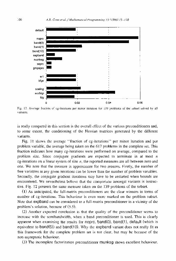
Fig. 12. Average fraction of cg-iterations per minor iteration lbr 139 problems of the subset solved by all v33"iRnts.

is really compared in this section is the overall effect of the various preconditioners and,

to some extent, the conditioning of the Hessian matrices generated by the different variants.

Fig. 11 shows the average "fraction of cg-iterations" per minor iteration and per

problem variable, the average being taken on the 617 problems in the complete set. This fraction indicates how many cg-iterations were performed on average, compared to the

problem size. Since conjugate gradients are expected to terminate in at most n cg-iterations on a linear system of size n, the reported measures are all between zero and

one. We note that the measure is approximate for two reasons. Firstly, the number of

free variables at any given iterations can be lower than the number of problem variables. Secondly, the conjugate gradient iterations may have to be restarted when bounds are encountered. We nevertheless believe that the comparison amongst variants is instruc-

tive. Fig. 12 presents the same measure taken on the 139 problems of the subset.

(1) As anticipated, the full-matrix preconditioners are the clear winners in terms of number of cg-iterations, This behaviour is even more marked on the problem subset.

Note that expband can be considered to a full-matrix preconditioner in a vicinity of the

problem's solution, because of (5.5). (2) Another expected conclusion is that the quality of the preconditioner seems to

increase with the semibandwidth, when a band preconditioner is used. This is clearly

apparent when examining the results for noprc, band(O), band(l), default (which is

equivalent to band(5)) and band(10). Why the expband variant does not really fit in

this framework for the complete problem set is not clear, but may be because of the

non-asymptotic behaviour.

(3) The incomplete factorization preconditioner munksg shows excellent behaviour.


Indeed its performance is nearly comparable to that of the full-matrix variants on the

complete problem set. (4) Solving the BQP accurately of course requires more cg-iterations, and we observe

this effect when comparing default and accbqp. This is especially noticeable on the

problems of the subset, because they are larger. (5) The scaled variant scaling is somewhat less efficient than the default unscaled

variant on the complete problem set, which is again an indication that scaling should not

be applied blindly to every problem. Its performance is however improved on the larger

problems of the subset. (6) The quasi-Newton approximations to the second derivatives do not seem to

generate matrices that are, on average, worse conditioned than their analytic counter- parts, as is shown by the comparable values for the default, bfgs and srl variants. The fact that gradients are estimated by differences in fog does not seem to considerably

impact the conditioning of the Hessian either, as can be seen by comparing this variant

with srl. (7) The reported measures are typically smaller for the subset than for the complete

problem set. This is anticipated as conjugate gradient solvers often require a number of iterations that is more dependent on conditioning and eigenvalue distribution than on system size. Increasing size therefore produce lower measures if one assume that the larger problems have an eigenvalue structure that is, on average, not worse than that of smaller ones.

7.4. Computational effort

We next compare our fifteen algorithmic variants on the basis of their requirements in CPU-time. Fig. 13 shows the average CPU-time (in seconds) required for solution, the

default

noprc band(O) band(l)

band(lO) oxpband munksg

seprc gmpsprc

semltf

srl bfgs

scaling accbqp

fdg

0 50 1 O0 I

150 200 250 300

Fig. 13. Average CPU-time for 617 problems solved by all variants.

102

7oo

A,R. Corm et al . /Mathematical Programming 73 (1996) 73-110

600

500

400

300

200

Poor

Fair [ ] ~ factoW

Good [ ] Excellent

100

default noprc band(l) ex]pband sep rc semfi'f srl accbqp band(0) band(10) munksg gmpsprc bfgs scaling fdg

Fig. 14. Ranking by CPU-time for 617 problems solved by all variants.

average being taken on the 617 problems in the complete set that were successfully solved by all methods. Fig. 14 presents a overall view of the relative ranking of the variants based on CPU-time. This figure was constructed in the same way as Fig. 8. Figs. 15 and 16 present the corresponding average and ranking results for the selected subset of test problems.

default

nopre band(0) band(l)

band(10) expband

munksg seprc

gmpsprc semltf

srl

bfgs

scaling accbqp

fdg

II i I

I I !11 i I I 1

I I I I I

�9 1 - i F i I I

0 200 400 600 800 1000 1200

Fig. 15. Average CPU-time for } 39 problems of the subset solved by all variants.

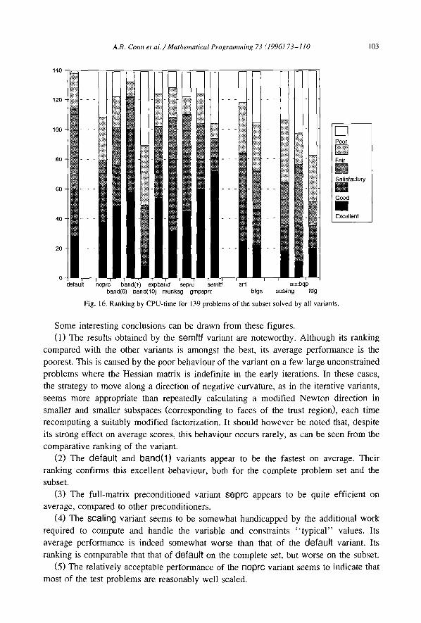
A.R. Corm et aL / Mathematical Prograrmning 73 (1996) 73-110 103

140

120

100

80

60

40

20

[ ] Poor [ ] Fair [ ] ~ factory

Good

Excellent

default noprc band(l) expband sep rc semltf srl accbqp band(O) band(lO) munksg gmpsprc bfgs scaling fdg

Fig. 16. Ranking by CPU-time for 139 problems of the subset solved by all variants.

Some interesting conclusions can be drawn from these figures. (1) The results obtained by the semltf variant are noteworthy. Although its ranking

compared with the other variants is amongst the best, its average performance is the poorest. This is caused by the poor behaviour of the variant on a few large unconstrained problems where the Hessian matrix is indefinite in the early iterations. In these cases, the strategy to move along a direction of negative curvature, as in the iterative variants, seems more appropriate than repeatedly calculating a modified Newton direction in smaller and smaller subspaces (corresponding to faces of the trust region), each time recomputing a suitably modified factorization. It should however be noted that, despite its strong effect on average scores, this behaviour occurs rarely, as can be seen from the comparative ranking of the variant.

(2) The default and band( l ) variants appear to be the fastest on average. Their ranking confirms this excellent behaviour, both for the complete problem set and the subset.

(3) The full-matrix preconditioned variant soprc appears to be quite efficient on average, compared to other preconditioners.

(4) The scaling variant seems to be somewhat handicapped by the additional work required to compute and handle the variable and constraints " typical" values. Its average performance is indeed somewhat worse than that of the default variant. Its ranking is comparable that that of default on the complete set, but worse on the subset.

(5) The relatively acceptable performance of the noprc variant seems to indicate that most of the test problems are reasonably well scaled.

104 A.R. Corm et al./Mathematical Programming 73 (1996) 73 llO

(6) The behaviour of banded preconditioners with varying semi-bandwidth is worth a comment. We already noted the good performance of the tridiagonal preconditioner (band(I)) and the default (band(5)), both on the complete problem set and on the subset. The band(10) variant uses more CPU-time as the advantage of improved

preconditioning is offset by the higher price of the preconditioner. The good performance of the expanding band variant expband, compared with band(] 0), seems to be

due to the general sparse storage scheme used, which is preferable to the band storage for matrices with higher bandwidth.

(7) The more costly iterations of accbqp clearly cause the relatively large average CPU-time of this variant on the complete problem set. However, as the expense of CPU-time is mostly confined to large problems, and as there are comparatively few such

problems in the complete test set, the method ranks reasonably highly. This observation

is strengthened by the relatively poor ranking of this variant for the large problems of the subset.

(8) Amongst the quasi-Newton variants, sr3 appears to be the most efficient. Its ranking is also consistently better than that of bfgs.

(9) The work involved in approximating the gradients by differences causes fdg to be slower than srl on average. This effect is enough to cause the relative ranking of fdg to fall substantially behind that of s r l .

7.5. Add i t iona l c o m m e n t s

We did not discuss above the relative number of unsuccessful iterations for each variant. This number is on ave r age below one per problem for each variant. It seems to indicate that the trust region management used in LANCELOT is adequate for handling a large class of nonlinear problems.

Besides its algorithmic choices, LANCELOT allows the user to select a number of non-algorithmic options, such as element and group derivative checking, level of printout and frequency at which intermediate data is saved for a possible subsequent restart. None of these options has a significant impact on the overall execution time of the package. The only observable increase in CPU-time occurs when a very detailed printout is required at every iteration of a large scale problem. As one would expect, this effect is slightly more marked for constrained cases, where the details of the major iterations have to be printed as well.

We finally indicate some weak points of LANCELOT (Release A) that we have observed in examining the detailed runs, but that cannot be inferred directly from the summaries presented above.

(1) When the number of inequality constraints is large compared with the number of variables, the package currently adds slack variables to transform all inequalities into equalities, which results in a substantial increase in the effective problem size. Although convergence is usually obtained, the computational effort can be relatively large compared with method that use inequality constraints directly (see [14], for instance). The authors are well aware of this aspect of their implementation, and have recently


given in [19] a method to overcome this difficulty, although it has not been incorporated in the software.

(2) No special provision is made in the present code for linear network constraints, or even for linear constraints. Again, LANCELOT seems to be robust in that convergence is obtained for problems with this kind of structure, but special purpose algorithms are often much more efficient (see [1,22,46,52,53], for instance).

(3) The ability of the generalized Cauchy point to determine the correct active set is disappointing in practice. In many examples, the correct active set is actually found in the conjugate gradient or direct matrix improvement beyond the GCP, at considerable cost. Although the GCP asymptotically identifies the correct active set as predicted by the theory (see [10], for instance), this is often at the end of a long calculation. A strategy treating the bounds through barrier functions (as proposed in [14]) might therefore be a useful alternative.

8. Conclusions

We first described the algorithms contained in Release A of the LANCELOT package for large-scale nonlinear optimization. We also analyzed the user-selectable variants. We finally presented and discussed the results of extensive numerical tests with these variants.

The main conclusions of these tests, as far as the package is concerned, are as follows.

(1) The package is capable of solving a wide class of nonlinear optimization problems, including many large-scale examples.

(2) The package is relatively more efficient for unconstrained and bound constrained problems and for generally constrained problems for which the number of constraints does not substantially exceed the problem dimension.

(3) The default algorithmic choice in the package appears to be both reliable and acceptably efficient, compared to other variants.

(4) Some algorithmic choices (automatic scaling, accurate solution of the inner BQP) should not be used automatically, but may provide excellent behaviour on some harder problems.

Beyond these conclusions relative to the LANCELOT package, our tests also reveal the following points of more general interest.

(1) The difficulty of solving a problem is more often linked to its degree of nonlinearity than to its size.

(2) The use of direct factorization appears to be most robust when used as preconditioners for a conjugate gradient linear solver.

(3) The use of exact second derivatives is recommended whenever available. How- ever, the partitioned symmetric-rank-one technique, as embedded in the package, gives very satisfactory reliability and efficiency (compared to other variants) when analytic second derivatives are not available.

106 A,R, Corm et al./Mathematical Programming 73 (1996) 73-110

(4) When analytical first derivatives are not available, finite difference approximations to the gradients coupled with SRI quasi-Newton Hessian updating is an acceptably

robust technique, even for large problems. (5) The use of full factorizations appears to be reliable for the class of problems

analyzed in this paper. It is however expected that this technique would appear less promising if even larger problems were considered. In contrast, banded preconditioners

would probably extend well to larger problems. Of course, only continued experience with LANCELOT will really show its strengths

and weaknesses. The authors very much hope to be informed by the users of the package

of the (undoubtedly many) aspects where improvements are possible. Progress is expected to come both from the point of view of the algorithms (see [14,17], for example) and from that of the implementation details themselves. It is also clear that

further comparisons with other packages are desirable, in particular to better assess the efficiency of LANCELOT in a wider context. The ongoing comparison with MINOS should thus provide useful additional conclusions, when completed. At this stage, the results discussed above certainly offer the hope that the software will prove useful in the

increasingly important arena of large-scale nonlinear optimization.

Acknowledgements

The authors are indebted to Michel Bierlaire and Didier Burton, whose help was invaluable in producing the graphics of this paper and in maintaining the workstation network during the 8 months of nearly uninterrupted computation required for obtaining the results presented here. Nick Gould is grateful to CERFACS, Toulouse, France, for the facilities which made some of this research possible. Thanks are also due to Ingrid Bongartz, Marc Breitfeld and Peihuang Chen for detecting and correcting mistakes in our test problems. Ingrid Bongartz furthermore provided valuable comments on a draft of the manuscript. The authors are grateful for the support provided for their travels across the Atlantic by NATO grant 890867. Finally, the anthors acknowledge the contribution of the editor, associate editor and of a referee, whose comments and reports

have been very stimulating. Current reports available from the second author by anonymous ftp from the directory

"pub / r epor t s " on camelot.cc.rl.ac.uk (internet 130.246.8.61) and from the third author from the directory "pub / repor t s " on thales.math.fundp.ac.be (internet 138.48.4.14).

Appendix

The purpose of this section is to report the details of what algorithmic options were used to solve the problem discussed in Section 7.1.2, when this proved possible, as well as the corresponding number of minor iterations, cg-iterations and CPU-time. These details are given in Table 4, where the two columns serve to identify the problem, the

A.R. Corm et al. /Mathematical Programming 73 (1996) 73-110

Table 4 Detailed algorithmic choices and performance for the problems solved using nonstandard variants

107

Problem n Basic Additional Minor cg CPU-time Note name variant specification iterations iterations (s)

AGG 163 seprc 266 76817 6013 (1) CHEMRCTA 5000 seprc scaling 35 64 760 CORKSCRW 4497 seprc 122 60078 40033 CORKSCRW 8997 seprc 126 2 1 5 5 0 2 264573 ERRINBAR 18 default 4053 30881 570 HS84 5 default 74 403 7 (2) HS93 6 default /.t o = 10 -2 44 75 4 HS99 7 default /~o = 10-5 32 28 3 (2) HSI03 7 default accbqp mad /.t o - 10 2518 34780 460 (2) HS116 13 seprc /x o = 10 -5 4108 15932 458 (2) LEWISPOL 6 default ,% = 10- ~0 I8 22 2 MARATOSB 2 default 1715 1286 144 NOMSQRT 529 seprc accbqp 225 4421 5239 NOMSQRT 1024 seprc accbqp 510 2 7 4 3 5 5 559376 OBSTCLAE 15625 default 5 7450 39588 OPTMASS 606 seprc /x o = 10 -4 3744 6268 2731 OPTMASS 1206 seprc iz o = 10 4 13320 25033 18644 OPTMASS 3006 seprc /z o = 1 0 - 4 44309 76825 149512 SVANBERG 5000 default 100 12985 46730 TENBARS4 18 default 2690 21031 372

third indicating the basic variant used and the fourth what further modification of this

variant have been specified, if any. When the name of another variant is mentioned in

this column, this means that the features of both the variants of columns three and four

are used. For instance, CHEMRCTA was solved by using the seprc variant (Schnabel-

Eskow preconditioning) with constraints and variables scaling, as specified in the variant

scal ing. Columns five, six and seven indicate the associated number of minor iterations,

cg-iterations and the CPU-time required for LANCELOT to terminate. The last column

refers to the following comments.

(1) The standard sep rc variant fails because the step generated by the algorithm is

insignificantly small at a point where the projected gradient is not small, but this seems

to be due to problem scaling and degeneracy. The optimal objective function produced

by MINOS ( - 3 5 9 9 1 7 6 7 . 2 9 ) is slightly worse than that produced by LANCELOT

( - 35 991 766.35) but its solution is closer to feasibility (constraint violation of the oraor

of 10 -23 for MINOS and of the order of 10 -7 for LANCELOT). ( 2 ) L A N C E L O T f a i l s because the s tep b e c o m e s t o o shor t . T h i s e x i t c o r r e s p o n d s to

the " s ta l l " situation described in Section 7.1.1. However, the optimal solution appears

to be found.

We do not report here on the four problems, HS99EXP, NGONE and the two cases

of LUBRIF, that we have not managed so far to solve using LANCELOT.

These results of Table 4 show that in most cases (AGG, CHEMRCTA, ERRINBAR,

HS84, HS93, HS99, HS103, H S l l 6 LEWISPOL, MARATOSB, NONMSQRT (n =

829), OPTMASS (n = 606 and 1206) and TENBARS4) a satisfactory solution could be

108 A.R. Connet a L / Mathematiea I Programming 73 (1996) 73-110

c o m p u t e d in r e a s o n a b l e t ime . O n l y the six r e m a i n i n g p r o b l e m s r e q u i r e d s u b s t a n t i a l l y

m o r e c o m p u t a t i o n a l e f f o r t fo r the i r so lu t ion .

References

[1] D.P. Ahlfeld, R.S. Dembo, J.M. Mulvey and S.A. Zenios, "'Nonlinear programming on generalized networks," ACM Transactions on Mathematical S ~ v a r e 13 (1987) 350-367.

[2} B.M. Averick, R.G. Carter and J.J. Mor•, "'The Minpack-2 test problem collection (preliminary version)," Technical Report ANL/MCS-TM-150, Argonne National Laboratory (Argonne, IL, 1991).

[3] B.M. Averick and J.J. Mor6, "'The Minpack-2 test problem collection," Technical Report ANL/MCS- TM- 157, Argonne National Laboratory (Argonne, 1L 1991).

[4] I. Bongartz, A.R. Corm, N. Gould and Ph.L. Toint. "' CUTE: Constrained and Unconstrained Testing Environment," ACM Transactions on Mathematical Software 21 (1995) 12 I - 160.

[5] A.G. Buckley, "Test functions for unconstrained minimization," Technical Report CS-3, Computing Science Division, Dalhousie University (Dalhousie, Canada, 1989).

[6] J.V. Burke and J.J. Mor6, "'On the identification of active constraints," SlAM Journal on Numerical Analysis 25 (1988) 1197-1211.

[7] J.V. Burke, J.J. Mord and G. Toraldo, "Convergence properties of trust region methods for linear and convex constraints," Mathematical Programming 47 (1990) 305-336.

[8] P.H. Calamai and J.J. Mor& "Projected gradient methods for linearly constrained problems," Mathemat- ical Programming 39 (1987) 93-116.

[9] A.R. Corm, N. Gould, M. Lescrenier and Ph.L. Toint, "'Performance of a multifrontal scheme for partially separable optimization," in: Advances in Optimization ate1 Numerical Analysis. Proceedings of the Sixth Workshop on Optimization and Numerical Analysis. Oaxaca, Mexico (Kluwer, Dordrecht, Netherlands, 1994) pp. 79-96.

[10] A.R. Corm, N. Gould and Ph.L. Toint, "Global convergence of a class of trust region algorithms for optimization with simple bounds," SlAM Journal on Numerical Analysis 25 (1988) 433-460. [See also same journal 26 (1989) 764-767.]

[1i] A.R. Corm, N. Gould and Ph.L. Toint, "'Testing a class of methods for solving minimization problems with simple bounds on the variables," Mathematics of Computation 50 (1988) 399-430.

[12] A.R. Corm, N. Gould and Ph.L. Toint, "An introduction to the structure of large scale nonlinear optimization problems and the LANCELOT project," in: R. Glowinski and A. Lichnewsky, eds., Computing Methods in Applied Sciences and Engineering (SIAM, Philadelphia, PA, 1990) pp. 42-51.

[13] A.R. Corm, N. Gould and Ph.L Toint, "A globally convergent augmented Lagrangian algorithm for optimization with general constraints and simple bounds," SIAM Journal on Ntonerical Analysis 28 (1991) 545-572.

[14] A.R. Corm, N. Gould and Ph.L. Toint, "'A globally convergent Lagrangian barrier algorithm for optimization with general inequality constraints and simple bounds," Mathematics of" Computation, to appear.

[15] A.R. Conn, N. Gould and Ph.L. Toint, LANCF:LOT: a Fortran Package for Large-Scale Nonlinear Optimization (Release A), Springer Series in Computational Mathematics, Vol. 17 (Springer, Berlin, 1992).

[16] A.R. Corm, N. Gould and Ph.L. Toint, "'On the number of inner iterations per outer iteration of a globally convergent algorithm for optimization with general nonlinear equality constraints and simple hounds," in: D.F Griffiths and G.A. Watson, eds., Proceedings of the 14th Biennal Numerical Analysis Conference Dundee 1991 (Longmans, London, 1992) pp. 49-68.

[17] A.R. Conn, N. Gould and Ph.L. Toint, "Convergence properties of minimization algorithms for convex constraints using a structured trust region," SlAM Journal on Optimization, to appear.

[t8] A.R. Corm, N. Gould and Ph.L Toint, "'Intensive numerical tests with LANCELOT (Release A): the complete results," Technical Report 92/15, Department of Mathematics, FUNDP (Namur, Belgium, 1992).

[19] A.R. Conn, N. Gould and Ph.L. Toint, "A note on exploiting structure when using slack variables," Mathematical Programming 67 (1994) 89-97.

A.R. Corm et al . / Mathematicul Programming 73 (1996)73-110 109

[20] A.R. Curtis and J.K. Reid, "'On the automatic scaling of matrices for Gaussian elimination," Journal of the Institute of Mathematics and its Applications 10 (1972) 118-124.

[21] R.S. Dembo, "'A primal truncated-newton algorithm with application to large-scale nonlinear network optimization," Technical Report 72, Yale School of Management (Yale University, New Haven, CT, 1984).

[22] R.S. Dembo, "The performance of NLPNET, a large scale nonlinear network optimizer," Mathematical Programming 26 (1986) 245-249.

[23] J.E. Dennis and R.B. Schnabel, Numerical Methods for Unconstrained Optimization and Nonlinear Equations (Prentice-Hall, Englewood Cliffs, N J, 1983).

[24] L.C.W. Dixon, "On automatic differentiation and continuous optimization," in: E. Spedicato, ed., Algorithms Jbr Continuous Optimization: the State of the Art (Kluwer, Dordrecht, 1994) pp. 501-513.

[25] I.S. Duff, A.M. Erisman and J.K. Reid, Direct Methods Jor Sparse Matrices (Clarendon Press, Oxford, 1986).

[26] I.S. Duff and J.K. Reid, "'MA27: A set of Fortran subroutines for solving sparse symmetric sets of linear equations," Report R-10533, AERE Harwell Laboratory (Harwell, UK, 1982).

[27] I.S. Duff and J.K. Reid, "The multifrontal solution of indefinite sparse symmetric linear equations," ACM Transactions on Mathematical Software 9 (1983) 302-325.

[28] R. Fletcher, Practical Methods of Optimization (Wiley, Chichester, 2nd ed., 1987). [29] A. George and J.W.-H. Liu, Computer Solution r Sparse Positive Definite Systems (Prentice-Hall,

Englewood Cliffs, NJ, 1981). [30] P.E. Gill, W. Murray, D.B. Poncel6on and M.A. Saunders, "'Preconditioners for indefinite systems

arising in optimization," SlAM Journal on Matrix Analysis and Applications 13 (1992) 292-311. [31] P.E. Gill, W. Murray and M.H. Wright, Practical Optimization (Academic Press, London, 1981). [32] G.H. Golub and C.F. Van Loan, Matrix Computations (Johns Hopkins University Press, Baltimore, MD,

2nd ed., 1989). [33] A. Griewank, "'Computational differentiation and optimization," in: J.R. Birge and K.G. Murty, eds.,

Mathematical Programming: State of the Art 1994 (The University of Michigan, Ann Arbor, MI, 1994) pp. 102-131.

[34] A. Griewank and Ph.L. Toint, "On the unconstrained optimization of partially separable functions," in: M.J.D. Powell, ed., Nonlinear Optimization 1981 (Academic Press, London. 1982) pp. 30t-312.

[35] M. Gulliksson, "Algorithms for nonlinear least squares with applications to orthogonal regression," Ph.D. Thesis, Institute of Information Processing, University of Ume~t (1990).

[36] W. Hock and K. Schittkowski, Test Examples .]or Nonlinear Programming Codes, Lectures Notes in Economics and Mathematical Systems Vol. 187 (Springer, Berlin, 1981).

[37] M.M. Kostreva, "Elasto-hydrodynamic lubrification: a non-linear complementarity problem," Interna- tional Journal for Numerical Methods in Fluids 4 (1984) 377-397.

[38] M. Lescrenier, "Convergence of trust region algorithms for optimization with bounds when strict complementarity does not hold," SlAM Journal on Numerical Analysis 28 (1991) 476-495.

[39] A. Lewis, private communication (1990). [40] J.J. Mor6, "Trust regions and projected gradients," in: M. Iri and K. Yajima, eds., System Modelling and

Optimization, Lecture Notes in Control and Information Sciences Vol. 113 (Springer, Berlin, 1988) pp. 1-13.

[41] J.J. Mor~, "A collection of nonlinear model problems," Technical Report ANL/MCS-P60-0289, Argonne National Laboratory (Argonne, IL, 1989).

[42] J.J. Mor6, B.S. Garbow and K.E. Hillstrom. "Testing unconstrained optimization software," ACM Transactions on Mathematical So,rare 7 ( 198 i) 17-41.

[43] J.J. Mor6 and G. Toraldo, "On the solution of large scale quadratic programming problems with bound constraints," SlAM Journal on Optimization 1 ( 1991 ) 93-113.

[44] N. Munksgaard, "Solving sparse symmetric systems of linear equations by preconditioned conjugate gradients," ACM Transactions on Mathematical Software 6 (1980) 206-219.

[45] B.A. Murtagh and M.A. Saunders, "'MINOS 5.1 USER'S GUIDE," Technical Report SOL83-20R, Department of Operations Research, Stanford University (Stanford, CA, 1987).

[46] A. Sartenaer, -A class of trust region methods for nonlinear network optimization problems," SIAM Journal on Optimization, 5 (1995) 379-407.

[47] K. Schittkowski, "'More Test Examples for Nonlinear Programming Codes," Lecture Notes in Eco- nomics and Mathematical Systems Vol. 282 (Springer, Berlin, 1987).

110 A.R. Corm et al. / Mathematical Programming 73 (1996) 73-110

[48] T. Schlick, "Modified Cholesky factorizations for sparse preconditioners,'" SIAM Journal on Scientific and Statistical Computing 14 (1993) 424-445.

[49] R.B. Sctmabel and E. Eskow, "A new modified Cholesky factorization," SIAM Journal on Scientific and Statistical Computing 11 (199I) 1136-1158.

[50] Ph.L. Toint, "'Test problems for partially separable optimization and results for the routine PSPMIN," Technical Report 83/4, Department of Mathematics, FUNDP (Namur, Belgium. 1983).

[51] Ph.L. Toint, "Global convergence of a class of trust region methods for nonconvex minimization in Hilbert space," IMA Journal of Numerical Analysis 8 (1988) 231-252.

[52] Ph.L. Toint and D. Tuyttens, "On large scale nonlinear network optimization," Mathematical Program- ruing 48 (1990) 125-159.

[53] Pb.L. Toint and D. Tuyttens, '~LSNNO: a Fortran subroutine for solving large scale nonlinear network optimization problems," ACM Transactions on Mathematical Software 18 (1992) 308-328.

Numerical experiments with the LANCELOT … · In this paper, we describe the algorithmic options...

Documents

Transcript of Numerical experiments with the LANCELOT … · In this paper, we describe the algorithmic options...