Chapter 11Numerical Differentiation

Differentiation is a basic mathematical operation with a wide range of applica-tions in many areas of science. It is therefore important to have good meth-ods to compute and manipulate derivatives. You probably learnt the basic rulesof differentiation in school — symbolic methods suitable for pencil-and-papercalculations. Such methods are of limited value on computers since the mostcommon programming environments do not have support for symbolic com-putations.

Another complication is the fact that in many practical applications a func-tion is only known at a few isolated points. For example, we may measure theposition of a car every minute via a GPS (Global Positioning System) unit, andwe want to compute its speed. When the position is known at all times (as amathematical function), we can find the speed by differentiation. But when theposition is only known at isolated times, this is not possible.

The solution is to use approximate methods of differentiation. In our con-text, these are going to be numerical methods. We are going to present severalsuch methods, but more importantly, we are going to present a general strategyfor deriving numerical differentiation methods. In this way you will not onlyhave a number of methods available to you, but you will also be able to developnew methods, tailored to special situations that you may encounter.

The basic strategy for deriving numerical differentiation methods is to evalu-ate a function at a few points, find the polynomial that interpolates the functionat these points, and use the derivative of this polynomial as an approximation tothe derivative of the function. This technique also allows us to keep track of theso-called truncation error, the mathematical error committed by differentiatingthe polynomial instead of the function itself. In addition to the truncation error,

251

there are also round-off errors, which are unavoidable when we use floating-point numbers to perform calculations with real numbers. It turns out that nu-merical differentiation is very sensitive to round-off errors, but these errors arequite easy to analyse.

The general idea of the chapter is to introduce the simplest method for nu-merical differentiation in section 11.1, with a complete error analysis. This mayappear a bit overwhelming, but it should not be so difficult since virtually all thedetails are included. You should therefore study this section carefully, and if youunderstand this, the simplest of the methods and its analysis, you should haveno problems understanding the others as well, since both the derivation and theanalysis is essentially the same for all the methods. The general strategy for de-riving and analysing numerical differentiation methods is then summarised insection 11.2. In the following sections we introduce three more differentiationmethods, including one for calculating second derivatives. For these methodswe just state the error estimates; the derivation of the estimates is left for theexercises. Note that the methods for numerical integration in Chapter 12 are de-rived and analysed in much the same way as the differentiation methods in thischapter.

11.1 Newton’s difference quotient

We start by introducing the simplest method for numerical differentiation, de-rive its error, and its sensitivity to round-off errors. The procedure used here forderiving the method and analysing the error is used over again in later sectionsto derive and analyse the other methods.

Let us first explain what we mean by numerical differentiation.

Problem 11.1 (Numerical differentiation). Let f be a given function that isknown at a number of isolated points. The problem of numerical differen-tiation is to compute an approximation to the derivative f ′ of f by suitablecombinations of the known function values of f .

A typical example is that f is given by a computer program (more specifi-cally a function, procedure or method, depending on your choice of program-ming language), and you can call the program with a floating-point argumentx and receive back a floating-point approximation of f (x). The challenge is tocompute an approximation to f ′(a) for some real number a when the only aidwe have at our disposal is the program to compute values of f .

252

11.1.1 The basic idea

Since we are going to compute derivatives, we must be clear about how they aredefined. The standard definition of f ′(a) is by a limit process,

f ′(a) = limh→0

f (a +h)− f (a)

h. (11.1)

In the following we will assume that this limit exists, in other words that f isdifferentiable at x = a. From the definition (11.1) we immediately have a nat-ural approximation of f ′(a): We simply pick a positive number h and use theapproximation

f ′(a) ≈ f (a +h)− f (a)

h. (11.2)

Recall that the straight line p1 that interpolates f at a and a +h (the secantbased at these points) is given by

p1(x) = f (a)+ f (a +h)− f (a)

h(x −a).

The derivative of this secant is exactly the right-hand side in (11.2) and corre-sponds to the secant’s slope. The approximation (11.2) therefore corresponds toapproximating f by the secant based at a and a +h, and using its slope as anapproximation to the slope of f at a, see figure 11.1.

The tangent to f at a has the same slope as f at a, so we may also obtainthe approximation (11.2) by considering the secant based at a and a +h as anapproximation to the tangent at a, see again figure 11.1.

Observation 11.2 (Newton’s difference quotient). The derivative of f at a canbe approximated by

f ′(a) ≈ f (a +h)− f (a)

h. (11.3)

This approximation is referred to as Newton’s difference quotient or just New-ton’s quotient.

An alternative to the approximation (11.3) is the left-sided version

f ′(a) ≈ f (a)− f (a −h)

h.

Not surprisingly, this approximation behaves similarly, and the analysis is alsocompletely analogous to that of the more common right-sided version.

In later sections, we will derive several formulas like (11.2). Which formula touse in a particular situation, and exactly how to apply it, will have to be decidedin each case.

253

a

f HaL

a+h

f Ha+hL

Figure 11.1. The secant of a function based at a and a +h, as well as the tangent at a.

Example 11.3. Let us test the approximation (11.3) for the function f (x) = sin xat a = 0.5 (using 64-bit floating-point numbers). In this case we know that theexact derivative is f ′(x) = cos x so f ′(a) ≈ 0.8775825619 with 10 correct digits.This makes it is easy to check the accuracy of the numerical method. We trywith a few values of h and find

h(

f (a +h)− f (a))/

h E( f ; a,h)

10−1 0.8521693479 2.5×10−2

10−2 0.8751708279 2.4×10−3

10−3 0.8773427029 2.4×10−4

10−4 0.8775585892 2.4×10−5

10−5 0.8775801647 2.4×10−6

10−6 0.8775823222 2.4×10−7

where E( f ; a,h) = f ′(a)−(f (a+h)− f (a)

)/h. We observe that the approximation

improves with decreasing h, as expected. More precisely, when h is reduced bya factor of 10, the error is reduced by the same factor.

11.1.2 The truncation error

Whenever we use approximations, it is important to try and keep track of theerror, if at all possible. To analyse the error in numerical differentiation, Tay-lor polynomials with remainders are useful. We start by doing a linear Taylor

254

expansion of f (a +h) about x = a which results in the relation

f (a +h) = f (a)+h f ′(a)+ h2

2f ′′(ξh), (11.4)

where ξh lies in the interval (a, a+h). This formula may be rearranged to give anexpression for the error,

f ′(a)− f (a +h)− f (a)

h=−h

2f ′′(ξh). (11.5)

This is often referred to as the truncation error of the approximation.

Example 11.4. Let us check that the error formula (11.5) agrees with the nu-merical values in example 11.3. We have f ′′(x) = −sin x, so the right-hand sidein (11.5) becomes

E(sin;0.5,h) = h

2sinξh ,

where ξh ∈ (0.5,0.5+h). We do not know the exact value of ξh , but for the valuesof h in question, we know that sin x is monotone on this interval. For h = 0.1 wetherefore have that the error must lie in the interval

[0.05sin0.5, 0.05sin0.6] = [2.397×10−2, 2.823×10−2],

and we see that the right end point of the interval is the maximum value of theright-hand side in (11.5).

When h is reduced by a factor of 10, the number h/2 is reduced by the samefactor, while ξh is restricted to an interval whose width is also reduced by a factorof 10. As h becomes even smaller, the number ξh will approach 0.5 so sinξh

will approach the lower value sin0.5 ≈ 0.479426. For h = 10−n , the error willtherefore tend to

10−n

2sin0.5 ≈ 0.2397

10n ,

which is in close agreement with the numbers computed in example 11.3.

The observation at the end of example 11.4 is true in general: If f ′′ is contin-uous, then ξh will approach a when h goes to zero. But even for small, positivevalues of h, the error in using the approximation f ′′(ξh) ≈ f ′′(a) is usually ac-ceptable. This is the case since we are almost always only interested in knowingthe approximate magnitude of the error, i.e., it is sufficient to know the errorwith one or two correct digits.

255

Observation 11.5. The truncation error when using Newton’s quotient to ap-proximate f ′(a) is given approximately by∣∣∣∣ f ′(a)− f (a +h)− f (a)

h

∣∣∣∣≈ h

2

∣∣ f ′′(a)∣∣ . (11.6)

An upper bound on the truncation error

For practical purposes, the approximation (11.6) is usually sufficient. But let usalso take the time to present a more precise argument. We will use a techniquefrom chapter 9 and derive an upper bound on the truncation error.

We go back to (11.5) and start by taking absolute values,∣∣∣∣ f ′(a)− f (a +h)− f (a)

h

∣∣∣∣= h

2

∣∣ f ′′(ξh)∣∣ .

We know that ξh is a number in the interval (a, a +h), so it is natural to replace| f ′′(ξh)| by its maximum in this interval. Here we must be a bit careful since thismaximum does not always exist. But recall from the Extreme value theorem thatif a function is continuous, then it always attains its maximum on any closedand bounded interval. It is therefore natural to include the end points of the in-terval (a, a+h) and take the maximum over [a, a+h]. This leads to the followinglemma.

Lemma 11.6. Suppose f has continuous derivatives up to order two near a.If the derivative f ′(a) is approximated by

f (a +h)− f (a)

h,

then the truncation error is bounded by

E( f ; a,h) =∣∣∣∣ f ′(a)− f (a +h)− f (a)

h

∣∣∣∣≤ h

2max

x∈[a,a+h]

∣∣ f ′′(x)∣∣ . (11.7)

11.1.3 The round-off error

So far, we have just considered the mathematical error committed when f ′(a) isapproximated by

(f (a+h)− f (a)

)/h. But what about the round-off error? In fact,

when we compute this approximation with small values of h we have to performthe one critical operation f (a +h)− f (a), i.e., subtraction of two almost equal

256

numbers, which we know from chapter 5 may lead to large round-off errors. Letus continue the calculations in example 11.3 and see what happens if we usesmaller values of h.

Example 11.7. Recall that we estimated the derivative of f (x) = sin x at a = 0.5and that the correct value with ten digits is f ′(0.5) ≈ 0.8775825619. If we checkvalues of h for 10−7 and smaller we find

h(

f (a +h)− f (a))/

h E( f ; a,h)

10−7 0. 8775825372 2.5×10−8

10−8 0.8775825622 −2.9×10−10

10−9 0.8775825622 −2.9×10−10

10−11 0.8775813409 1.2×10−6

10−14 0.8770761895 5.1×10−4

10−15 0.8881784197 −1.1×10−2

10−16 1.110223025 −2.3×10−1

10−17 0.000000000 8.8×10−1

This shows very clearly that something quite dramatic happens. Ultimately,when we come to h = 10−17, the derivative is computed as zero.

Round-off errors in the function values

Let us see if we can explain what happened in example 11.7. We will go throughthe explanation for a general function, but keep the concrete example in mind.

The function value f (a) will usually not be representable exactly in the com-puter and will therefore be replaced by the nearest floating-point number whichwe denote f (a). We then know from lemma 5.21 that the relative error in this ap-proximation will be bounded by 5×2−53 since floating-point numbers are repre-sented in binary (β= 2) with 53 bits for the significand (m = 53). In other words,if we set

ε1 = f (a)− f (a)

f (a), (11.8)

we have

|ε1| ≤ 5×2−53 ≈ 6×10−16. (11.9)

This means that |ε1| is the relative error, while ε1 itself is the signed relative error.Note that ε1 will depend both on a and f , and in practice, there will usually

be better upper bounds on ε1 than the one in (11.9). In the following we willdenote the least upper bound by ε∗.

257

Notation 11.8. The maximum relative error that occurs when real numbersare represented by floating-point numbers, and there is no underflow or over-flow, is denoted by ε∗.

We will see later in this chapter that a reasonable estimate for ε∗ is ε∗ ≈ 7×10−17. We note that equation (11.8) may be rewritten in a form that will be moreconvenient for us.

Observation 11.9. Suppose that f (a) is computed with 64-bit floating-pointnumbers and that no underflow or overflow occurs. Then the computed valuef (a) satisfies

f (a) = f (a)(1+ε1) (11.10)

where |ε1| ≤ ε∗, and ε1 depends on both a and f .

The computation of f (a +h) is of course also affected by round-off error, soin total we have

f (a) = f (a)(1+ε1), f (a +h) = f (a +h)(1+ε2), (11.11)

where |εi | ≤ ε∗ for i = 1, 2. Here we should really write ε2 = ε2(h), because theexact round-off error in f (a +h) will inevitably depend on h in an apparentlyrandom way.

Round-off errors in the computed derivative

The next step is to see how these errors affect the computed approximation off ′(a). Recall from example 5.12 that the main source of round-off in subtractionis the replacement of the numbers to be subtracted by the nearest floating-pointnumbers. We therefore consider the computed approximation to be

f (a +h)− f (a)

h,

and ignore the error in the division by h. If we insert the expressions (11.11), andalso make use of equation (11.5), we obtain

f ′(a)− f (a +h)− f (a)

h= f ′(a)− f (a +h)− f (a)

h− f (a +h)ε2 − f (a)ε1

h

=−h

2f ′′(ξh)− f (a +h)ε2 − f (a)ε1

h,

(11.12)

258

where ξh ∈ (a, a+h). This shows that the total error in the computed approxima-tion to the derivative consists of two parts: The truncation error that we derivedin the previous section, plus the last term on the right in (11.12), which is due tothe round-off when real numbers are replaced by floating-point numbers. Thetruncation error is proportional to h and therefore tends to 0 when h tends to0. The error due to round-off however, is proportional to 1/h and therefore be-comes large when h tends to 0.

In observation 11.5 we obtained an approximate expression for the trunca-tion error, for small values of h, by replacing ξh by a. When h is small we mayalso assume that f (a +h) ≈ f (a) so (11.12) leads to the approximate error esti-mate

f ′(a)− f (a +h)− f (a)

h≈−h

2f ′′(a)− ε2 −ε1

hf (a). (11.13)

The most uncertain term in (11.13) is the difference ε2 − ε1. Since we do noteven know the signs of the two numbers ε1 and ε2, we cannot estimate this dif-ference accurately. But we do know that both numbers represent relative errorsin floating-point numbers, so the magnitude of each is about 10−17. If they areof opposite signs, this magnitude may be doubled, so we replace the differenceε2 − ε1 by 2ε̃(h) to emphasise the dependence on h. The error (11.13) then be-comes

f ′(a)− f (a +h)− f (a)

h≈−h

2f ′′(a)− 2ε̃(h)

hf (a). (11.14)

Let us check if this agrees with the computations in examples 11.3 and 11.7.

Example 11.10. For large values of h the first term on the right in (11.14) willdominate the error, and we have already seen that this agrees very well with thecomputed values in example 11.3. The question is how well the numbers in ex-ample 11.7 can be modelled when h becomes smaller.

To investigate this, we denote the left-hand side of (11.14) by E( f ; a,h) andsolve for ε̃(h),

ε̃(h) ≈− h

2 f (a)

(E( f ; a,h)+ h

2f ′′(a)

).

From example 11.7 we have corresponding values of h and E( f ; a,h) which allowus to estimate ε̃(h) (recall that f (x) = sin x and a = 0.5 in this example). If we do

259

-20 -15 -10 -5

-10

-8

-6

-4

-2

Figure 11.2. Numerical approximation of the derivative of f (x) = sin x at x = 0.5 using Newton’s quotient,see lemma 11.6. The plot is a log10-log10 plot which shows the logarithm to base 10 of the absolute value ofthe total error as a function of the logarithm to base 10 of h, based on 200 values of h. The point −10 on thehorizontal axis therefore corresponds h = 10−10, and the point −6 on the vertical axis corresponds to an errorof 10−6. The solid line is a plot of the error estimate g (h) given by (11.15).

this we can augment the table on page 257 with an additional column

h(

f (a +h)− f (a))/

h E( f ; a,h) ε̃(h)

10−7 0. 8775825372 2.5×10−8 −7.6×10−17

10−8 0.8775825622 −2.9×10−10 2.8×10−17

10−9 0.8775825622 −2.9×10−10 5.5×10−19

10−11 0.8775813409 1.2×10−6 −1.3×10−17

10−14 0.8770761895 5.1×10−4 −5.3×10−18

10−15 0.8881784197 −1.1×10−2 1.1×10−17

10−16 1.110223025 −2.3×10−1 2.4×10−17

10−17 0.000000000 8.8×10−1 −9.2×10−18

We observe that all these values are considerably smaller than the upper limit6× 10−16 in (11.9). (Note that in order to compute ε̃(h) correctly for h = 10−7,you need to use the more accurate value 2.4695×10−8 for the error in this case.)

Figure 11.2 shows plots of the error. The numerical approximation has beencomputed for the values h = 10−z , for z = 0, . . . , 20 in steps of 1/10, and theabsolute value of the total error plotted in a log-log plot. The errors are shownas isolated dots, and the function

g (h) = h

2sin0.5+ε 2

hsin0.5 (11.15)

with ε = 7 × 10−17 is shown as a solid graph. This corresponds to adding the

260

absolute value of the truncation error and the round-off error, even in the casewhere they have opposite signs. It appears that the choice of ε makes g (h) areasonable upper bound on the error so we may consider this to be a decentestimate of ε∗.

The estimates (11.13) and (11.14) give the approximate error with sign. Ingeneral, it is more convenient to consider the absolute value of the error. Start-ing with (11.13), we then have∣∣∣ f ′(a)− f (a +h)− f (a)

h

∣∣∣≈ ∣∣∣−h

2f ′′(a)− ε2 −ε1

hf (a)

∣∣∣≤ h

2| f ′′(a)|+ |ε2 −ε1|

h| f (a)|

≤ h

2| f ′′(a)|+ |ε2|+ |ε1|

h| f (a)|

≤ h

2| f ′′(a)|+ 2ε(h)

h| f (a)|

where we used the triangle inequality in the first and second inequality, and ε(h)is the largest of the two numbers |ε1| and |ε2|.

Observation 11.11. Suppose that f and its first two derivatives are continu-ous near a. When the derivative of f at a is approximated by Newton’s dif-ference quotient (11.3), the error in the computed approximation is roughlybounded by∣∣∣∣ f ′(a)− f (a +h)− f (a)

h

∣∣∣∣. h

2

∣∣ f ′′(a)∣∣+ 2ε(h)

h

∣∣ f (a)∣∣ , (11.16)

where ε(h) is the largest of the relative errors in f (a) and f (a +h), and thenotation α.β indicates that α is approximately smaller than β.

An upper bound on the total error

The . notation is vague mathematically, so we include a more precise error es-timate.

Theorem 11.12. Suppose that f and its first two derivatives are continuousnear a. When the derivative of f at a is approximated by

f (a +h)− f (a)

h,

261

the error in the computed approximation is bounded by∣∣∣∣ f ′(a)− f (a +h)− f (a)

h

∣∣∣∣≤ h

2M1 + 2ε∗

hM2, (11.17)

whereM1 = max

x∈[a,a+h]

∣∣ f ′′(x)∣∣ , M2 = max

x∈[a,a+h]

∣∣ f (x)∣∣ .

Proof. To get to (11.17) we start with (11.12), take absolute values, and use thetriangle inequality a number of times. We also replace

∣∣ f ′′(ξh)∣∣ by its maximum

on the interval [a, a +h], and we replace f (a) and f (a +h) by their commonmaximum on [a, a +h]. The details are:

∣∣∣ f ′(a)− f (a +h)− f (a)

h

∣∣∣= ∣∣∣h

2f ′′(ξh)− f (a +h)ε2 − f (a)ε1

h

∣∣∣≤ h

2| f ′′(ξh)|+ | f (a +h)ε2 − f (a)ε1|

h

≤ h

2| f ′′(ξh)|+ | f (a +h)||ε2|+ | f (a)||ε1|

h

≤ h

2M1 + M2|ε2|+M2|ε1|

h

= h

2M1 + |ε2|+ |ε1|

hM2

≤ h

2M1 + 2ε∗

hM2.

(11.18)

11.1.4 Optimal choice of h

Figure 11.2 indicates that there is an optimal value of h which minimises thetotal error. We can find a decent estimate for this h by minimising the upperbound in one of the error estimates (11.16) or (11.17). In practice it is easiest touse (11.16) since the two numbers M1 and M2 in (11.17) depend on h (althoughwe could insert some upper bound which is independent of h).

The right-hand side of (11.16) contains the term ε(h) whose exact depen-dence on h is very uncertain. We therefore replace ε(h) by the upper bound ε∗.This gives us the error estimate

e(h) = h

2

∣∣ f ′′(a)∣∣+ 2ε∗

h

∣∣ f (a)∣∣ . (11.19)

To find the value of h which minimises this expression, we differentiate with

262

respect to h and set the derivative to zero. We find

e ′(h) =∣∣ f ′′(a)

∣∣2

− 2ε∗

h2

∣∣ f (a)∣∣ .

If we solve the equation e ′(h) = 0, we obtain the approximate optimal value.

Lemma 11.13. Let f be a function with continuous derivatives up to order 2.If the derivative of f at a is approximated as in lemma 11.6, then the valueof h which minimises the total error (truncation error + round-off error) isapproximately

h∗ ≈ 2

√ε∗

∣∣ f (a)∣∣√∣∣ f ′′(a)∣∣ .

It is easy to see that the optimal value of h is the value that balances the twoterms in (11.19), i.e., the truncation error and the round-off error are equal.

Example 11.14. Based on example 11.7, we saw above that a good value of ε∗

is 7× 10−17. Let us check what the optimal value of h is in this case. We havef (x) = sin x and a = 0.5 so

h∗ = 2pε= 2

√7×10−17 ≈ 1.7×10−8.

For this value of h we find

sin(0.5+h∗)− sin0.5

h∗ = 0.877582555644682,

and the error in this case is about 6.2×10−9. It turns out that roughly all h in theinterval [3.2×10−9,2×10−8] give an error of about the same magnitude whichshows that the determination of h∗ is quite robust.

Exercises

1 In this exercise we are going to numerically compute the derivative of f (x) = ex at a = 1using Newton’s quotient as described in observation 11.2. The exact derivative to 20 digitsis

f ′(1) ≈ 2.7182818284590452354.

a) Compute the approximation(

f (1+h)− f (1))/h to f ′(1). Start with h = 10−4, and

then gradually reduce h. Also compute the error, and determine an h that givesclose to minimal error.

263

b) Determine the optimal h as described in Lemma 11.13 and compare with the valueyou found in (a).

2 When deriving the truncation error given by (11.7) it is not obvious what the degree of theTaylor polynomial in (11.4) should be. In this exercise you are going to try and increaseand reduce the degree of the Taylor polynomial and see what happens.

a) Redo the Taylor expansion in (11.4), but use the Taylor polynomial of degree 2. Fromthis try and derive an error formula similar to (11.5).

b) Repeat (a), but use a Taylor polynomial of degree 0, i.e., just a constant.

c) Why can you conclude that the linear Taylor polynomial and the error term in (11.5)is correct?

11.2 Summary of the general strategy

Before we continue, let us sum up the derivation and analysis of the Newton’sdifference quotient in section 11.1, since this is standard for all differentiationmethods.

The first step is to derive the numerical method. In section 11.1 this was verysimple since the method came straight out of the definition of the derivative.Just before observation 11.2 we indicated that the method can also be derivedby approximating f by a polynomial p and using p ′(a) as an approximation tof ′(a). This is the general approach that we will use below.

Once the numerical method is known, we estimate the mathematical errorin the approximation, the truncation error. This we do by performing Taylorexpansions with remainders. For numerical differentiation methods which pro-vide estimates of a derivative at a point a, we replace all function values at pointsother than a by Taylor polynomials with remainders. There may be a challengein choosing the correct degree of the Taylor polynomial, see exercise 11.1.2.

The next task is to estimate the total error, including the round-off error. Weconsider the difference between the derivative to be computed and the com-puted approximation, and replace the computed function evaluations by ex-pressions like the ones in observation 11.9. This will result in an expressioninvolving the mathematical approximation to the derivative. This can be sim-plified in the same way as when the truncation error was estimated, with theaddition of an expression involving the relative round-off errors in the functionevaluations. These estimates can then be simplified to something like (11.16)or (11.17). As a final step, the optimal value of h can be found by minimising thetotal error.

264

Procedure 11.15. The following is a general procedure for deriving numericalmethods for differentiation:

1. Interpolate the function f by a polynomial p at suitable points.

2. Approximate the derivative of f by the derivative of p. This makes itpossible to express the approximation in terms of function values of f .

3. Derive an estimate for the error by expanding the function values (otherthan the one at a) in Taylor series with remainders.

4. Derive an estimate of the round-off error by assuming that the relativeerrors in the function values are bounded by ε∗. By minimising the totalerror, an optimal step length h can be determined.

Exercises

1 Determine an approximation to the derivative f ′(a) using the function values f (a), f (a +h) and f (a + 2h) by interpolating f by a quadratic polynomial p2 at the three points a,a +h, and a +2h, and then using f ′(a) ≈ p ′

2(a).

11.3 A symmetric version of Newton’s quotient

The numerical differentiation method in section 11.1 is not symmetric about a,so let us try and derive a symmetric method.

11.3.1 Derivation of the method

We want to find an approximation to f ′(a) using values of f near a. To obtaina symmetric method, we assume that f (a −h), f (a), and f (a +h) are knownvalues, and we want to find an approximation to f ′(a) using these values. Thestrategy is to determine the quadratic polynomial p2 that interpolates f at a−h,a and a +h, and then we use p ′

2(a) as an approximation to f ′(a).We start by writing p2 in Newton form,

p2(x) = f [a −h]+ f [a −h, a](x − (a −h))

+ f [a −h, a, a +h](x − (a −h))(x −a). (11.20)

We differentiate and find

p ′2(x) = f [a −h, a]+ f [a −h, a, a +h](2x −2a +h).

265

Setting x = a yields

p ′2(a) = f [a −h, a]+ f [a −h, a, a +h]h.

To get a practically useful formula we must express the divided differences interms of function values. If we expand the second divided difference we obtain

p ′2(a) = f [a−h, a]+ f [a, a +h]− f [a −h, a]

2hh = f [a, a +h]+ f [a −h, a]

2. (11.21)

The two first order differences are

f [a −h, a] = f (a)− f (a −h)

h, f [a, a +h] = f (a +h)− f (a)

h,

and if we insert this in (11.21) we end up with

p ′2(a) = f (a +h)− f (a −h)

2h.

We note that the approximation to the derivative given by p ′2(a) agrees with the

slope of the secant based at a −h and a +h.

Lemma 11.16 (Symmetric Newton’s quotient). Let f be a given function, andlet a and h be given numbers. If f (a−h), f (a), f (a+h) are known values, thenf ′(a) can be approximated by p ′

2(a) where p2 is the quadratic polynomial thatinterpolates f at a −h, a, and a +h. The approximation is given by

f ′(a) ≈ p ′2(a) = f (a +h)− f (a −h)

2h, (11.22)

and agrees with the slope of the secant based at a −h and a +h.

The symmetric Newton’s quotient is illustrated in figure ??. The derivative off at a is given by the slope of the tangent, while the approximation defined byp ′

2(a) is given by the slope of tangent of the parabola at a (which is the same asthe slope of the secant of f based at a −h and a +h).

Let us test this approximation on the function f (x) = sin x at a = 0.5 sowe can compare with the original Newton’s quotient that we discussed in sec-tion 11.1.

Example 11.17. We test the approximation (11.22) with the same values of h asin examples 11.3 and 11.7. Recall that f ′(0.5) ≈ 0.8775825619 with 10 correct

266

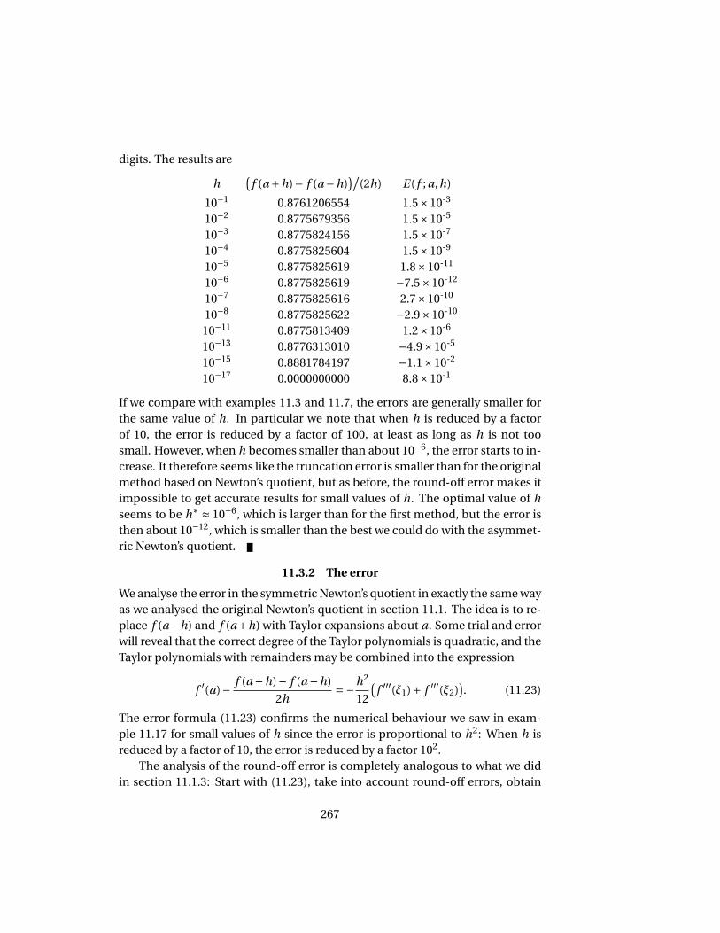
digits. The results are

h(

f (a +h)− f (a −h))/

(2h) E( f ; a,h)

10−1 0.8761206554 1.5×10-3

10−2 0.8775679356 1.5×10-5

10−3 0.8775824156 1.5×10-7

10−4 0.8775825604 1.5×10-9

10−5 0.8775825619 1.8×10-11

10−6 0.8775825619 −7.5×10-12

10−7 0.8775825616 2.7×10-10

10−8 0.8775825622 −2.9×10-10

10−11 0.8775813409 1.2×10-6

10−13 0.8776313010 −4.9×10-5

10−15 0.8881784197 −1.1×10-2

10−17 0.0000000000 8.8×10-1

If we compare with examples 11.3 and 11.7, the errors are generally smaller forthe same value of h. In particular we note that when h is reduced by a factorof 10, the error is reduced by a factor of 100, at least as long as h is not toosmall. However, when h becomes smaller than about 10−6, the error starts to in-crease. It therefore seems like the truncation error is smaller than for the originalmethod based on Newton’s quotient, but as before, the round-off error makes itimpossible to get accurate results for small values of h. The optimal value of hseems to be h∗ ≈ 10−6, which is larger than for the first method, but the error isthen about 10−12, which is smaller than the best we could do with the asymmet-ric Newton’s quotient.

11.3.2 The error

We analyse the error in the symmetric Newton’s quotient in exactly the same wayas we analysed the original Newton’s quotient in section 11.1. The idea is to re-place f (a−h) and f (a+h) with Taylor expansions about a. Some trial and errorwill reveal that the correct degree of the Taylor polynomials is quadratic, and theTaylor polynomials with remainders may be combined into the expression

f ′(a)− f (a +h)− f (a −h)

2h=−h2

12

(f ′′′(ξ1)+ f ′′′(ξ2)

). (11.23)

The error formula (11.23) confirms the numerical behaviour we saw in exam-ple 11.17 for small values of h since the error is proportional to h2: When h isreduced by a factor of 10, the error is reduced by a factor 102.

The analysis of the round-off error is completely analogous to what we didin section 11.1.3: Start with (11.23), take into account round-off errors, obtain

267

a relation similar to (11.12), and then derive the error estimate through a stringof equalities and inequalities as in (11.18). The result is a theorem similar totheorem 11.12.

Theorem 11.18. Let f be a given function with continuous derivatives up toorder three, and let a and h be given numbers. Then the error in the symmet-ric Newton’s quotient approximation to f (a),

f ′(a) ≈ f (a +h)− f (a −h)

2h,

including round-off error and truncation error, is bounded by∣∣∣∣∣ f ′(a)− f (a +h)− f (a −h)

2h

∣∣∣∣∣≤ h2

6M1 + ε∗

hM2, (11.24)

where

M1 = maxx∈[a−h,a+h]

∣∣ f ′′′(x)∣∣ , M2 = max

x∈[a−h,a+h]

∣∣ f (x)∣∣ . (11.25)

The most important feature of this theorem is that it shows how the errordepends on h. The first term on the right in (11.24) stems from the truncationerror (11.23) which clearly is proportional to h2, while the second term corre-sponds to the round-off error and depends on h−1 because we divide by h whencalculating the approximation.

It may be a bit surprising that the truncation error is smaller for the symmet-ric Newton’s quotient than for the asymmetric one, since both may be viewed ascoming from a secant approximation to f . The reason is that in the symmetriccase, the secant is just a special case of a parabola which is generally a betterapproximation than a straight line.

In practice, the interesting values of h will usually be so small that there isvery little error in using the approximations

M1 = maxx∈[a−h,a+h]

∣∣ f ′′′(x)∣∣≈ ∣∣ f ′′′(a)

∣∣ , M2 = maxx∈[a−h,a+h]

∣∣ f (x)∣∣≈ ∣∣ f (a)

∣∣ ,

in (11.24), particularly since we are only interested in the magnitude of the errorwith only 1 or 2 digits of accuracy. If we make these simplifications we obtain aslightly simpler error estimate.

268

-15 -10 -5

-12

-10

-8

-6

-4

-2

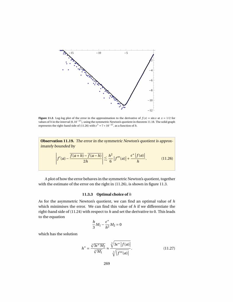
Figure 11.3. Log-log plot of the error in the approximation to the derivative of f (x) = sin x at x = 1/2 forvalues of h in the interval [0,10−17], using the symmetric Newton’s quotient in theorem 11.18. The solid graphrepresents the right-hand side of (11.26) with ε∗ = 7×10−17, as a function of h.

Observation 11.19. The error in the symmetric Newton’s quotient is approx-imately bounded by∣∣∣∣∣ f ′(a)− f (a +h)− f (a −h)

2h

∣∣∣∣∣. h2

6

∣∣ f ′′′(a)∣∣+ ε∗

∣∣ f (a)∣∣

h. (11.26)

A plot of how the error behaves in the symmetric Newton’s quotient, togetherwith the estimate of the error on the right in (11.26), is shown in figure 11.3.

11.3.3 Optimal choice of h

As for the asymmetric Newton’s quotient, we can find an optimal value of hwhich minimises the error. We can find this value of h if we differentiate theright-hand side of (11.24) with respect to h and set the derivative to 0. This leadsto the equation

h

3M1 − ε∗

h2 M2 = 0

which has the solution

h∗ =3p

3ε∗M23p

M1≈

3√

3ε∗∣∣ f (a)

∣∣3√∣∣ f ′′′(a)

∣∣ . (11.27)

269

At the end of section 11.1.4 we saw that a reasonable value for ε∗ was ε∗ = 7×10−17. The optimal value of h in example 11.17, where f (x) = sin x and a = 0.5,then becomes h = 4.6×10−6. For this value of h the approximation is f ′(0.5) ≈0.877582561887 with error 3.1×10−12.

Exercises

1 In this exercise we are going to check the symmetric Newton’s quotient and numericallycompute the derivative of f (x) = ex at a = 1, see exercise 11.1.1. Recall that the exactderivative with 20 correct digits is

f ′(1) ≈ 2.7182818284590452354.

a) Compute the approximation(

f (1+h)− f (1−h))/(2h) to f ′(1). Start with h = 10−3,

and then gradually reduce h. Also compute the error, and determine an h that givesclose to minimal error.

b) Determine the optimal h given by (11.27) and compare with the value you found in(a).

2 Determine f ′(a) numerically using the two asymmetric Newton’s quotients

fr (x) = f (a +h)− f (a)

h, fl (x) = f (a)− f (a −h)

h

as well as the symmetric Newton’s quotient. Also compute and compare the relative errorsin each case.

a) f (x) = x2; a = 2; h = 0.01.

b) f (x) = sin x; a =π/3; h = 0.1.

c) f (x) = sin x; a =π/3; h = 0.001.

d) f (x) = sin x; a =π/3; h = 0.00001.

e) f (x) = 2x ; a = 1; h = 0.0001.

f ) f (x) = x cos x; a =π/3; h = 0.0001.

3 In this exercise we are going to derive the error estimate (11.24). For this it is a good ideato use the derivation in sections 11.1.2 and 11.1.3 as a model, and try and follow the samestrategy.

a) Derive the relation (11.23) by replacing f (a−h) and f (a+h) with appropriate Taylorpolynomials with remainders around x = a.

b) Estimate the total error by replacing the values f (a −h) and f (a +h) by the near-est floating-point numbers f (a −h) and f (a +h). The result should be a relationsimilar to equation (11.12).

c) Find an upper bound on the total error by using the same steps as in (11.18).

4 a) Show that the approximation to f ′(a) given by the symmetric Newton’s quotient isthe average of the two asymmetric quotients

fr (x) = f (a +h)− f (a)

h, fl (x) = f (a)− f (a −h)

h.

270

b) Sketch the graph of the function

f (x) = −x2 +10x −5

4

on the interval [0,6] together with the three secants associated with the three ap-proximations to the derivative in (a) (use a = 3 and h = 2). Can you from this judgewhich approximation is best?

c) Determine the three difference quotients in (a) numerically for the function f (x)using a = 3 and h1 = 0.1 and h2 = 0.001. What are the relative errors?

d) Show that the symmetric Newton’s quotient at x = a for a quadratic function f (x) =ax2 +bx + c is equal to the derivative f ′(a).

5 Use the symmetric Newton’s quotient and determine an approximation to the derivativef ′(a) in each case below. Use the values of h given by h = 10−k k = 4,5, . . . ,12 and comparethe relative errors. Which of these values of h gives the smallest error? Compare with theoptimal h predicted by (11.27).

a) The function f (x) = 1/(1+cos(x2)) at the point a =π/4.

b) The function f (x) = x3 +x +1 at the point a = 0.

11.4 A four-point differentiation method

The asymmetric and symmetric Newton’s quotients are the two most commonlyused methods for approximating derivatives. Whenever possible, one wouldprefer the symmetric version whose truncation error is proportional to h2. Thismeans that the error goes to 0 more quickly than for the asymmetric version, aswas clearly evident in examples 11.3 and 11.17. In this section we derive anothermethod for which the truncation error is proportional to h4. This also illustratesthe procedure 11.15 in a more complicated situation.

The computations below may seem overwhelming, and have in fact beendone with the help of a computer to save time and reduce the risk of miscal-culations. The method is included here just to illustrate that the principle forderiving both the method and the error terms is just the same as for the simplerNewton’s quotient.

11.4.1 Derivation of the method

We want better accuracy than the symmetric Newton’s quotient which was basedon interpolation with a quadratic polynomial. It is therefore natural to base theapproximation on a cubic polynomial, which can interpolate four points. Wehave seen the advantage of symmetry, so we choose the interpolation points

271

x0 = a −2h, x1 = a −h, x2 = a +h, and x3 = a +2h. The cubic polynomial thatinterpolates f at these points is

p3(x) = f (x0)+ f [x0, x1](x −x0)+ f [x0, x1, x2](x −x0)(x −x1)

+ f [x0, x1, x2, x3](x −x0)(x −x1)(x −x2),

and its derivative is

p ′3(x) = f [x0, x1]+ f [x0, x1, x2](2x −x0 −x1)

+ f [x0, x1, x2, x3]((x −x1)(x −x2)+ (x −x0)(x −x2)+ (x −x0)(x −x1)

).

If we evaluate this expression at x = a and simplify (this is quite a bit of work),we find that the resulting approximation of f ′(a) is

f ′(a) ≈ p ′3(a) = f (a −2h)−8 f (a −h)+8 f (a +h)− f (a +2h)

12h. (11.28)

11.4.2 The error

To estimate the error, we expand the four terms in the numerator in (11.28) inTaylor polynomials of degree 4 with remainders. We then insert these into theformula for p ′

3(a) and obtain an analog to equation 11.12,

f ′(a)− f (a −2h)−8 f (a −h)+8 f (a +h)− f (a +2h)

12h=

h4

45f (v)(ξ1)− h4

180f (v)(ξ2)− h4

180f (v)(ξ3)+ h4

45f (v)(ξ4),

where ξ1 ∈ (a −2h, a), ξ2 ∈ (a −h, a), ξ3 ∈ (a, a +h), and ξ4 ∈ (a, a +2h). We cansimplify the right-hand side and obtain an upper bound on the truncation errorif we replace the function values by upper bounds. The result is∣∣∣∣ f ′(a)− f (a −2h)−8 f (a −h)+8 f (a +h)− f (a +2h)

12h

∣∣∣∣≤ h4

18M (11.29)

whereM = max

x∈[a−2h,a+2h]

∣∣ f (v)(x)∣∣ .

The round-off error is derived in the same way as before. The quantities weactually compute are

f (a −2h) = f (a −2h)(1+ε1), f (a +2h) = f (a +2h)(1+ε3),

f (a −h) = f (a −h)(1+ε2), f (a +h) = f (a +h)(1+ε4).

272

-15 -10 -5

-15

-10

-5

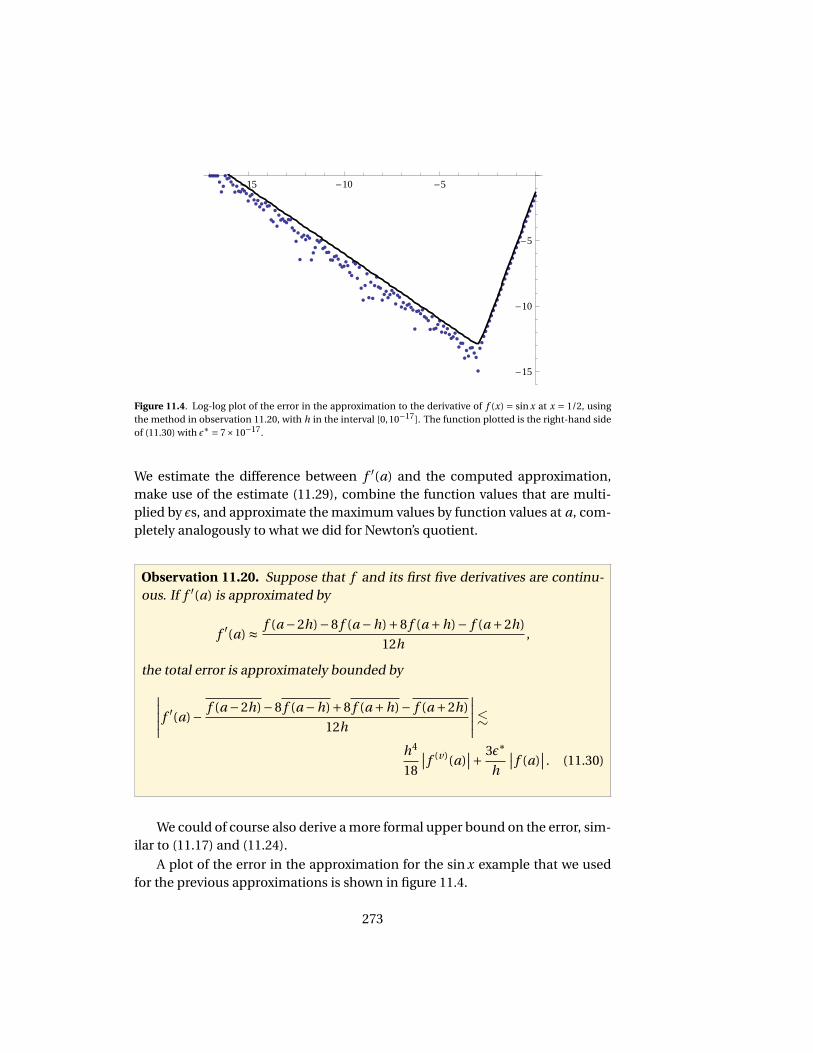
Figure 11.4. Log-log plot of the error in the approximation to the derivative of f (x) = sin x at x = 1/2, usingthe method in observation 11.20, with h in the interval [0,10−17]. The function plotted is the right-hand sideof (11.30) with ε∗ = 7×10−17.

We estimate the difference between f ′(a) and the computed approximation,make use of the estimate (11.29), combine the function values that are multi-plied by εs, and approximate the maximum values by function values at a, com-pletely analogously to what we did for Newton’s quotient.

Observation 11.20. Suppose that f and its first five derivatives are continu-ous. If f ′(a) is approximated by

f ′(a) ≈ f (a −2h)−8 f (a −h)+8 f (a +h)− f (a +2h)

12h,

the total error is approximately bounded by∣∣∣∣∣ f ′(a)− f (a −2h)−8 f (a −h)+8 f (a +h)− f (a +2h)

12h

∣∣∣∣∣.h4

18

∣∣ f (v)(a)∣∣+ 3ε∗

h

∣∣ f (a)∣∣ . (11.30)

We could of course also derive a more formal upper bound on the error, sim-ilar to (11.17) and (11.24).

A plot of the error in the approximation for the sin x example that we usedfor the previous approximations is shown in figure 11.4.

273

From observation 11.20 we can compute the optimal value of h by differen-tiating the right-hand side with respect to h and setting it to zero. This leads tothe equation

2h3

9

∣∣ f (v)(a)∣∣− 3ε∗

h2

∣∣ f (a)∣∣= 0

which has the solution

h∗ =5√

27ε∗∣∣ f (a)

∣∣5√

2∣∣ f (v)(a)

∣∣ . (11.31)

For the example f (x) = sin x and a = 0.5 the optimal value of h is h∗ ≈ 8.8×10−4.The actual error is then roughly 10−14.

Exercises

1 In this exercise we are going to check the four-point method and numerically compute thederivative of f (x) = ex at a = 1. For comparison, the exact derivative to 20 digits is

f ′(1) ≈ 2.7182818284590452354.

a) Compute the approximation(

f (a−2h)−8 f (a−h)+8 f (a+h)− f (a+2h))/(12h) to

f ′(1). Start with h = 10−3, and then gradually reduce h. Also compute the error, anddetermine an h that gives close to minimal error.

b) Determine the optimal h given by (11.31) and compare with the experimental valueyou found in (a).

2 Derive the estimate (11.29), starting with the relation just preceding (11.29).

11.5 Numerical approximation of the second derivative

We consider one more method for numerical approximation of derivatives, thistime of the second derivative. The approach is the same: We approximate f by apolynomial and approximate the second derivative of f by the second derivativeof the polynomial. As in the other cases, the error analysis is based on expansionin Taylor series.

11.5.1 Derivation of the method

Since we are going to find an approximation to the second derivative, we haveto approximate f by a polynomial of degree at least two, otherwise the secondderivative is identically 0. The simplest is therefore to use a quadratic polyno-mial, and for symmetry we want it to interpolate f at a −h, a, and a +h. The

274

resulting polynomial p2 is the one we used in section 11.3 and it is given in equa-tion (11.20). The second derivative of p2 is constant, and the approximation off ′(a) is

f ′′(a) ≈ p ′′2 (a) = f [a −h, a, a +h].

The divided difference is easy to expand.

Lemma 11.21 (Three-point approximation of second derivative). The secondderivative of a function f at a can be approximated by

f ′′(a) ≈ f (a +h)−2 f (a)+ f (a −h)

h2 . (11.32)

11.5.2 The error

Estimation of the error follows the same pattern as before. We replace f (a −h)and f (a+h) by cubic Taylor polynomials with remainders and obtain an expres-sion for the truncation error,

f ′′(a)− f (a +h)−2 f (a)+ f (a −h)

h2 =−h2

24

(f (i v)(ξ1)+ f (i v)(ξ2)

), (11.33)

where ξ1 ∈ (a −h, a) and ξ2 ∈ (a, a +h).The round-off error can also be estimated as before. Instead of computing

the exact values, we actually compute f (a −h), f (a), and f (a +h), which arelinked to the exact values by

f (a −h) = f (a −h)(1+ε1), f (a) = f (a)(1+ε2), f (a +h) = f (a +h)(1+ε3),

where |εi | ≤ ε∗ for i = 1, 2, 3. We can then derive a relation similar to (11.12), andby reasoning as in (11.18) we end up with an estimate of the total error.

Theorem 11.22. Suppose f and its first three derivatives are continuous neara, and that f ′′(a) is approximated by

f ′′(a) ≈ f (a +h)−2 f (a)+ f (a −h)

h2 .

Then the total error (truncation error + round-off error) in the computed ap-proximation is bounded by∣∣∣∣∣ f ′′(a)− f (a +h)−2 f (a)+ f (a −h)

h2

∣∣∣∣∣≤ h2

12M1 + 3ε∗

h2 M2, (11.34)

275

-8 -6 -4 -2

-8

-6

-4

-2

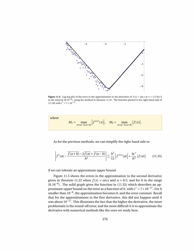
Figure 11.5. Log-log plot of the error in the approximation to the derivative of f (x) = sin x at x = 1/2 for hin the interval [0,10−8], using the method in theorem 11.22. The function plotted is the right-hand side of(11.30) with ε∗ = 7×10−17.

whereM1 = max

x∈[a−h,a+h]

∣∣∣ f (i v)(x)∣∣∣ , M2 = max

x∈[a−h,a+h]

∣∣ f (x)∣∣ .

As for the previous methods, we can simplify the right-hand side to

∣∣∣∣∣ f ′′(a)− f (a +h)−2 f (a)+ f (a −h)

h2

∣∣∣∣∣. h2

12

∣∣∣ f (i v)(a)∣∣∣+ 3ε∗

h2

∣∣ f (a)∣∣ (11.35)

if we can tolerate an approximate upper bound.

Figure 11.5 shows the errors in the approximation to the second derivativegiven in theorem 11.22 when f (x) = sin x and a = 0.5, and for h in the range[0,10−8]. The solid graph gives the function in (11.35) which describes an ap-proximate upper bound on the error as a function of h, with ε∗ = 7×10−17. For hsmaller than 10−8, the approximation becomes 0, and the error constant. Recallthat for the approximations to the first derivative, this did not happen until hwas about 10−17. This illustrates the fact that the higher the derivative, the moreproblematic is the round-off error, and the more difficult it is to approximate thederivative with numerical methods like the ones we study here.

276

11.5.3 Optimal value of h

As before, we find the optimal value of h by minimising the right-hand side of(11.35). To do this we find the derivative with respect to h and set it to 0,

h

6

∣∣ f ′′′(a)∣∣− 6ε∗

h3

∣∣ f (a)∣∣= 0.

Observation 11.23. The upper bound on the total error (11.34) is minimisedwhen h has the value

h∗ =4√

36ε∗∣∣ f (a)

∣∣4√∣∣ f (i v)(a)

∣∣ . (11.36)

When f (x) = sin x and a = 0.5 this gives h∗ = 2.2×10−4 if we use the valueε∗ = 7×10−17. Then the approximation to f ′′(a) =−sin a is −0.4794255352 withan actual error of 3.4×10−9.

Exercises

1 We use our standard example f (x) = e3 and a = 1 to check the 3-point approximation tothe second derivative given in (11.32). For comparison recall that the exact second deriva-tive to 20 digits is

f ′′(1) ≈ 2.7182818284590452354.

a) Compute the approximation(

f (a−h)−2 f (a)+ f (a+h))/(h2) to f ′′(1). Start with h =

10−3, and then gradually reduce h. Also compute the actual error, and determinean h that gives close to minimal error.

b) Determine the optimal h given by (11.36) and compare with the value you deter-mined in (a).

2 In this exercise you are going to do the error analysis of the three-point method in moredetail. As usual the derivation in sections 11.1.2 and 11.1.3 may be useful as a guide.

a) Derive the relation (11.33) by performing the appropriate Taylor expansions of f (a−h) and f (a +h).

b) Starting from (11.33), derive the analog of relation (11.12).

c) Derive the estimate (11.34) by following the same recipe as in (11.18).

3 This exercise illustrates a different approach to designing numerical differentiation meth-ods.

a) Suppose that we want to derive a method for approximating the derivative of f at awhich has the form

f ′(a) ≈ c1 f (a −h)+ c2 f (a +h), c1,c2 ∈R.

277

We want the method to be exact when f (x) = 1 and f (x) = x. Use these conditionsto determine c1 and c2.

b) Show that the method in (a) is exact for all polynomials of degree 1, and compare itto the methods we have discussed in this chapter.

c) Use the procedure in (a) and (b) to derive a method for approximating the secondderivative of f ,

f ′′(a) ≈ c1 f (a −h)+ c2 f (a)+ c3 f (a +h), c1,c2,c3 ∈R,

by requiring that the method should be exact when f (x) = 1, x and x2. Do yourecognise the method?

d) Show that the method in (c) is exact for all cubic polynomials.

278