NUMERICAL DETERMINATION OF ELECTRIC FIELD AROUND · PDF filenumerical determination of...

Journal of Science and Arts Year 12, No. 4(21), pp. 487-496, 2012

ORIGINAL PAPER

NUMERICAL DETERMINATION OF ELECTRIC FIELD AROUND A HIGH VOLTAGE ELECTRICAL OVERHEAD LINE

ELENA OTILIA VIRJOGHE1, DIANA ENESCU1, MIHAIL-FLORIN STAN1,

COSMIN COBIANU1 _________________________________________________

Manuscript received: 02.10.2012; Accepted paper: 20.11.2012;

Published online: 01.12.2012.

Abstract. This paper proposes a mathematical model of electric field caused by high voltage conductors of electric power transmission systems using the finite elements method. The numerical computation of electric field around of a high voltage 110 kV electrical overhead line is analyzed. The six conductors of a 110 kV transposed high voltage transmission line with double circuit are considered. The spectrum of electric field intensity close to the overhead electric power line and the studied body are analyzed using the ANSYS Multiphysics software package. The results obtained by simulation confirm that the electrostatic field computation for the conductor system and a human body lead to an accurate result. The used method can be useful in the design of the transmission power lines for estimating the insulation distance.

Keywords: electric field, high voltage electrical overhead lines, numerical simulation, Finite Elements Method.

1. INTRODUCTION The high voltage overhead lines can be considered as electromagnetical perturbation

sources. These perturbations are received by the neighbour circuits, the environment and the human body. Overhead electric power lines are needful for the transmission of electricity from power plants to consumers. Their operation produces electrical effects which affect the devices, equipments, systems close to lines operating under voltage as well as the human body exposure to these effects [1]. The parameter which characterizes the biological effects of human body exposure is the electric field intensity, at the point where the body is studied. It is very important to predict the electric field intensity that can affect the personnel operating on the power lines, determining the values of the electric field parameters around a three-phase electrical overhead line. Due to difficulty and burden in time of performing electric field measurement, numerical calculation can be applied to evaluate the electric field distribution.

The calculus of the potential V against the earth and the electrical field intensity E around a three-phase high voltage overhead electrical line with double circuit has been made by using the finite elements method (FEM). This method is one of the most popular numerical methods used for computer simulation. The FEM was used for the first time in the field of structural analysis. The method was applied to electromagnetic problems since 1968. Like the finite difference method, the finite element method is useful in solving differential equations [2]. The strong point of the FEM in comparison with other numerical methods in engineering applications is the ability to handle nonlinear, time-dependent and circular geometry

1 Valahia University of Targoviste, Electrical Engineering Faculty, 130024 Targoviste, Romania. E-mail: [email protected].

ISSN: 1844 – 9581 Physics Section

mailto:[email protected]

Numerical determination of … Elena Otilia Virjoghe et. al.

488

problems. The finite difference method represents the solution region by array of grid points but its application becomes difficult with problems having irregularly shaped boundaries. Such problems can be handled more easily using the finite element method. Therefore, this method is suitable for solving the problem involving electric field effects around the transmission line caused by circular cross-section of high voltage conductors [3]. This method assures sufficient accuracy of electric field computation and has a very good flexibility when the system geometry is complicate.

2. ANALYSIS OF ELECTRIC PROBLEMS BY FEM

2.1. ELECTRIC FIELD AND POTENTIAL FORMULATION

The electric field intensity is given by: E

VE

(1)

The divergence of the electric field density D

is related to the charge density ρ as follows:

Ddiv

(2)

Combining Eqs. (1) and (2) and introducing the dielectric permittivity ε and the

connection law in electric field, the Poissons’s equations describing the electrostatic potential becomes [4]:

V (3) 2.2. ELECTRIC ENERGY FUNCTIONAL

Among the various numerical techniques, the finite element medhod has a dominant position because it is versatile, having a strong interchangeability and can be incorporated into standard programs [5]. FEM is based on the fact that the physical systems stabilize at the minimum level of energy. Electric field calculation involves determining the electric scalar potential function V that minimizes the functional:

D SSNNv

EVdSVdfdDVEdDVF

N

01 )( (4)

where ΣN is the boundary surface with Neumann conditions, fN is function defined by the Neumann boundary condition, D is the volume of the proposed region, ρv is the electric charge density within volume v, ρS is surface electric charge density and S is surface of discontinuity in region of computing D. The necessary condition for stationarity of the functional involves:

www.josa.ro Physics Section

Numerical determination of … Elena Otilia Virjoghe et. al. 489

0)(

)()(1

SSNNv

D

SSNNv

D

VdSVdfdDVVgradD

VdSVdfdDVEDVF

N

N

(5)

In the computation domain, if the volume of the proposed region D is a linear,

isotropic, homogeneous body, without permanent polarization, the functional expression of the electrostatic field is:

nD

v Vdn

VdDVgradVVF

N n

2

1 2)(

(6)

In 3D problems in Cartesian coordinates (x, y, z), the expression of the energy

functional is:

D

NNv

N

VdzyxgdxdydzVz

V

y

V

x

VVF ),,(

2)(

222

1

(7)

where

Nn

Vg N

(8)

is the function defined by the Neumann boundary condition [5].

In bi-dimensional (2D) problems, the plane parallel electrostatic field in Cartesian coordinates (x, y) has the functional expression:

D

NNv

N

VdyxgdxdyVy

V

x

VVF ),(

2)(

22

1

(9)

The last term does not appear in (9), if the node is not on the inhomogeneous

boundary of Neumann. The general equation of energy in an electric field becomes [6]:

D

v dxdyVyV

xV

VF 22

1 2)(

(10)

In the FEM, the volume of the proposed region is divided into “m” small triangular

elements where their sides form a grid with “n” nodes. The potential function is then approximated by:

n

iii VrfrV

1)()( (11)



490

where Vi is the electric potential of node i, r is any point on the proposed region, fi(r) is called the shape function having the feature that any fi(r) is equal to unit at the location of node i and zero at the other nodes [7]:

jiforrf

jiforrf

i

i

0)(

1)( (12)

Substituting Eq. (11) into Eq. (10), the approximate energy is presented by W*, which

is minimized under the following conditions:

niVW

i,...,2,10

(13)

A system of equations whose unknowns are the electric potential values in the nodes

of the mesh is obtained. The electric field intensity within each element is obtained using the gradient expression as follows [7]:

n

i

miimm fVVE

1)( (14)

The finite elements analysis of any problem involves basically four steps [2]:

to discretize the solution region into a finite number of subdomains or elements; to derive the governing equations for a typical element; to assemble all the elements in the solution region; to solve the obtained equation system.

3. NUMERICAL ANALYSIS USING ANSYS Numerical simulation is realized using the finite element package ANSYS. This

program is based on the finite element method for solving Maxwell’s equations and can be used for modeling electromagnetic fields where the field is electrostatic, magnetostatic, with eddy currents, time-invariant or time-harmonic and with permanent magnets [8].

The procedure for carrying out an electrostatic analysis consists of the following main steps: create the physics environment, build and mesh the model and assign physics attributes to each region within the model, apply boundary conditions and loads (excitation), obtain the solution, review the results.

Consider a system consisting of 6 conductors (double circuit) with 3 conductors on each circuit. The conductors are located at a height of 20 m from earth. Each conductor has a diameter of 30 mm and is located at a distance of 3.6 meters and 5 meters (central conductors) of the tower of power line. The human body has a height of 1.8 m. The following regions with the properties are defined: human body, with relative permittivity εr=700 air, with relative permittivity εr=1.

The power lines are the bare conductors of Aluminum Conductor Steel Reinforced (ACSR) type, having the conductivity σ= 0.8 .10-7 S/m and the relative permittivity εr= 3.5 [3, 9]. Phases 1, 2 and 3 are at the electric potential of 110 kV and earth is at the reference electric potential 0 V.



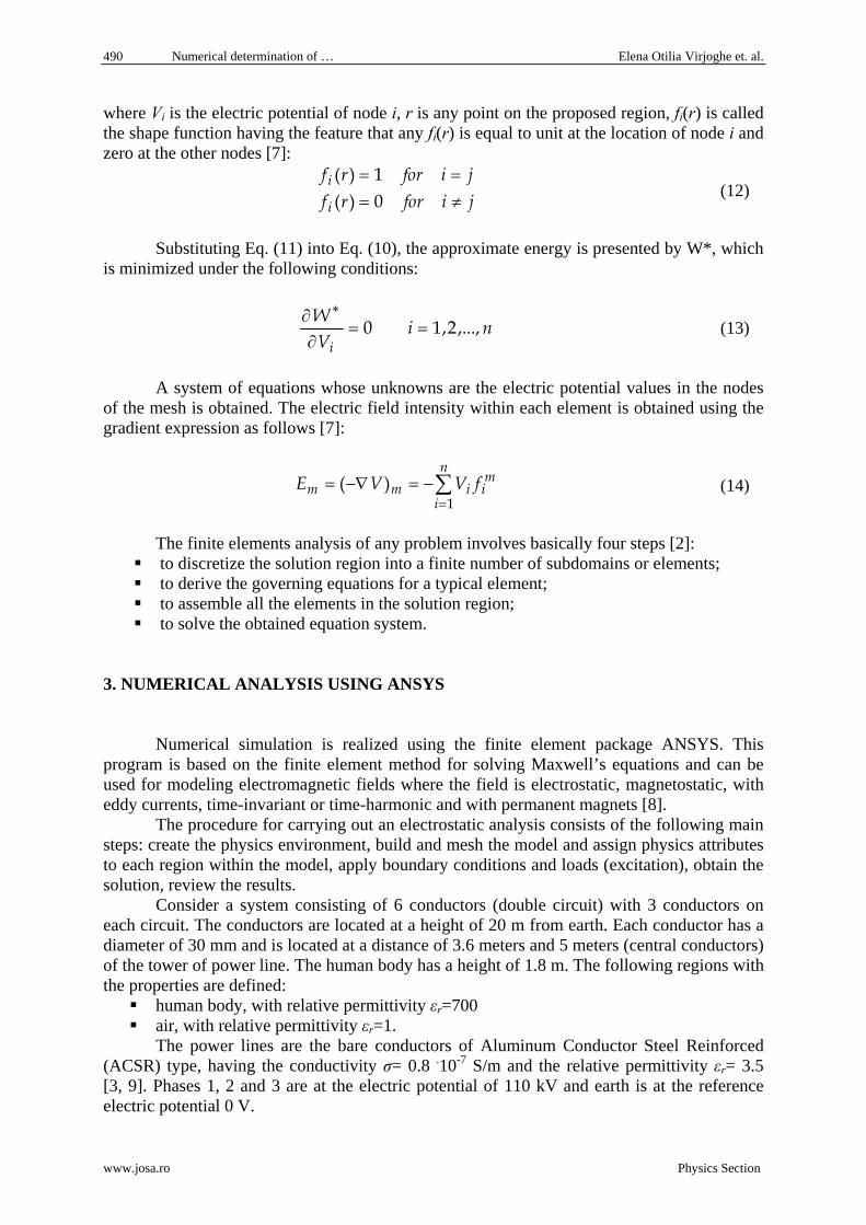
To define the physics environment for analysis, it is necessary to enter in the ANSYS preprocessor (PREP7) and to establish a mathematical simulation model of the physical problem [8]. First of all, the following steps are presented: set GUI Preferences, define the analysis title, define element types and options, define element coordinate systems, set real constants and define a system of units, define material properties [10]. ANSYS includes a variety of elements which can be used in modeling the electromagnetic phenomenon [8]. Element types establish the physics of the problem domain. Depending on the nature of the problem, several element types for modeling the different physics regions in the model have to be defined [10]. In this application, for modeling the electrostatic field a PLANE121 element was chosen, which allows two-dimensional modeling of the electric field for planar and symmetric problems (Fig. 1).

Fig. 1. PLANE121 element description.

The element is defined by eight nodes and orthotropic material properties. The

element has one degree of freedom and voltage at each node. This element is based on the electric scalar potential formulation, and it is applicable to 2D electrostatic and time-harmonic quasi-static electric field analyses. A triangular-shaped element may be formed by defining the same node number for nodes K, L and O [8]. The next step in the preprocessor phase is mesh generation and load applying upon the elements. We used a mesh with 7199 nodes and 3548 triangular elements. The finite element mesh of the system with six conductors is shown in Fig. 2.

1

X

Y

ZCâmpul electric generat de o LEA de 110 kV

JAN 28 201213:48:59

ELEMENTS

Fig. 2. Meshing the model with triangular elements.

The boundary conditions and loads to a 2D electrostatic analysis are applied, both on

the plane model (key points, lines, and areas) and on the finite element model (nodes and elements). The ANSYS program automatically transfers loads applied to the model to the mesh during solution [8]. There are several methods for solving the system of equations in



492

ANSYS: Sparse solver (default), Frontal solver, Jacobi Conjugate Gradient (JCG) solver, JCG out-of-memory solver, Incomplete Cholesky Conjugate Gradient (ICCG) solver, Preconditioned Conjugate Gradient solver (PCG), PCG out-of-memory solver.

The primary unknowns are nodal values of the electric potential and their derivatives are the secondary unknowns (electric field intensity and electric flux density).

3. SIMULATION AND RESULTS

In ANSYS there is a graphical program that displays the resulting fields in the form of contour and density plots. The program also allows the user to inspect the field at arbitrary points, as well as evaluate a number of different integrals and plot various quantities of interest along user-defined contours [8]. The distribution of electric potential is shown in Fig.3.

1

MN

MX

X

Y

Z

Câmpul electric generat de o LEA de 110 kV

012031

2406336094

4812560156

7218884219

96250110000

JAN 28 201214:05:07

NODAL SOLUTION

STEP=1SUB =1TIME=1VOLT (AVG)RSYS=0SMX =110000

Fig. 3. Distribution of electric potential.

The presence of a person changes the electric field configuration as seen in Fig. 4. The

electric field intensity increases in the conductors. The maximum value of the electric field is obtained around the bottom conductors. In this region, the electric field intensity has a maximum of 346.9 kV/m. Around the central conductors, the electric field intensity has a value of 114.7 kV/m and around the top conductors, the electric field value is 76. 9 kV/m.

1

MN X

Y

Z


012031

2406336094

4812560156

7218884219

96250110000

JAN 28 201214:18:13

NODAL SOLUTION

STEP=1SUB =1TIME=1VOLT (AVG)RSYS=0SMX =110000

Fig. 4. Distribution of electric potential (detail with human body).



The distribution of the electric field intensity is shown in Fig. 5. The electric field intensity at head level has a value higher than the value obtained from the ankles. In the arm region at a distance of 1.5 m above earth, the electric field intensity value is 3149 V/m and in the head region at a distance of 1.8 m above earth, the electric field intensity value is 4659 V/m. The distribution of electric field intensity around human body is shown in Fig. 6.

1

MNMX


.226E-0937944

75889113833

151778189722

227666265611

303555346920

JAN 28 201214:08:47

NODAL SOLUTION

STEP=1SUB =1TIME=1EFSUM (AVG)RSYS=0SMN =.226E-09SMX =346920

Fig. 5. Distribution of electric field intensity (detail conductors).

1

X

Y

Z


.226E-0937944

75889113833

151778189722

227666265611

303555346920

JAN 28 201214:10:25

NODAL SOLUTION

STEP=1SUB =1TIME=1EFSUM (AVG)RSYS=0SMN =.226E-09SMX =346920

Fig. 6. Distribution of electric field intensity (detail human body).

1

MNMX


.200E-14.336E-06

.672E-06.101E-05

.134E-05.168E-05

.202E-05.235E-05

.269E-05.307E-05

JAN 28 201214:11:56

NODAL SOLUTION

STEP=1SUB =1TIME=1DSUM (AVG)RSYS=0SMN =.200E-14SMX =.307E-05

Fig. 7. Distribution of electric flux density (detail conductors).



494

Fig. 7 shows the distribution of electric flux density around the conductors and Fig. 8 shows the distribution of electric flux density around the human body. Electric flux density is a vector field, which is independent of the medium. The electric flux is a quantitative expression of the number of lines passing through a surface.

1

X

Y

Z


.200E-14.336E-06

.672E-06.101E-05

.134E-05.168E-05

.202E-05.235E-05

.269E-05.307E-05

JAN 28 201214:13:11

NODAL SOLUTION

STEP=1SUB =1TIME=1DSUM (AVG)RSYS=0SMN =.200E-14SMX =.307E-05

Fig. 8. Distribution of electric flux density (detail human body).

The path for the displayed charts is chosen between two points placed symmetrical

one from another on the arms. It is also possible to save the plotted results in EMF format (Extended Metafile). Figs. 9 and 10 show the chart of the electric potential versus the distance as well as the electric field intensity versus the distance.

1

73.015

75.225

77.435

79.645

81.855

84.065

86.275

88.485

90.695

92.905

95.113

0.15

.3.45

.6.75

.91.05

1.21.35

1.5

DIST


JAN 28 201214:32:03

POST1

STEP=1SUB =1TIME=1PATH PLOTNOD1=1752NOD2=1755VOLT

Fig. 9. The electric potential versus the distance.

1

27.053

339.293

651.533

963.773

1276.013

1588.253

1900.493

2212.733

2524.973

2837.213

3149.455

0.15

.3.45

.6.75

.91.05

1.21.35

1.5

DIST


JAN 28 201214:37:49

POST1

STEP=1SUB =1TIME=1PATH PLOTNOD1=1752NOD2=1755EFSUM

Fig. 10. The electric field intensity versus the distance.



The electric field in installation is limited by the safety distances regarding the conductors [11, 12]. In different countries, there are different limit values. In Romania, the following prescribed values depend on the location of the power line: 5 kV/m in inhabited zones, 7 kV/m in crossing roads and 10 kV/m in all other cases [1]. The electric field intensity generated by the 110 kV overhead lines does not exceed the limit values, as seen in Figs. 9 and 10. It can be considered that the maximum electric field intensity at ground level is between 0.8 and 2.5 kV/m per 100 kV voltage line. The insulation distance estimation with values of nominal voltage make the highest electric field intensity found in the environment to be under 10 kV/m, even if transmission lines have a nominal voltage of 700 kV. Value of 10 kV/m electric field intensity is used as the design size of high voltage power lines [1].

4. CONCLUSIONS The electric field produced by overhead transmission lines for a given configuration is

directly proportional with the nominal voltage line and geometrical factors, such as the relative position of the conductors and their height above the ground [11, 12]. This paper proposes a mathematical model of electric field caused by high voltage conductors of electric power transmission systems using the finite elements method. The numerical computation of electric field around of a high voltage 110 kV electrical overhead line is analyzed. The six conductors of 110 kV transposed high voltage transmission line with double circuit are considered. The spectrum of electric field intensity close to the overhead electric power line and the studied human body are analyzed using the ANSYS program. The results obtained by simulation confirm that the electrostatic field computation for the conductor system and a human body lead to an accurate result. Method of calculation presented can be useful in the design of a transmission power lines for insulation distance estimation. This could mean that this method of numerical simulation approach can be used to predict the electric field generated by high voltage overhead power lines.

REFERENCES

[1] Dragan, G., Tehnica tensiunilor inalte, vol. III, Ed. Academiei Romane, Bucuresti, 2003.

[2] Malik, B., Ghosh, S., Ghosh, S., Electric field calculations by numerical techniques - Thesis, Department of Electrical Engineering National Institute of Technology, Rourkela, India, 2009.

[3] Isaramongkolrak, A., Kulworawanichpong, T., Pao-la-or, P., Finite element approach to electric field distribution resulting from phase-sequence orientation of a double-circuit high voltage transmission line, Proceedings of the 8th WSEAS International Conference on Electric Power Systems, High Voltages, Electric Machines (Power’08), Venice, Italy, November 21-23, 2008.

[4] Vassiliki T. Kontargyri, V.T., Ioannis F. Gonos, I.F., Stathopulos, I.A., Measurement and simulation of the electric field of high voltagesuspension insulators, European Transactions on Electrical Power, Euro. Trans. Electr. Power 2009.

[5] Fireteanu, V., Numerical modelling of electromagnetic fields in electrotechnic devices, Master course notes, Politehnica University of Bucharest, 1998.




496

[6] Silvester, P.P., Ferrari, R.L. Finite Elements for Electrical Engineers, Cambridge University Press, 2nd Edition, 1990.

[7] Faiz, J., Ojaghi, M., Int. J. Engng Ed., 18(3), 344, 2002. [8] ANSYS Guide Documentation. [9] Tupsie, S., Isaramongkolrak, A., Pao-la-or, P., International Journal of Electrical and

Computer Engineering, 5(4), 227, 2010. [10] Virjoghe, O.E., Enescu, D., Ionel, M., Arcing chamber optimization of DC Current-

Limiting Circuit Breaker Using FEM, Proceedings of the 9th WSEAS/IASME International Conference on Electric Power Systems, High Voltages, Electric Machines (Power’09), Genova, Italy, October 17-19, 2009, pp. 208-213, ISSN:1790-5117, ISBN: 978-960-474-130-4.

[11] Virjoghe, E.O., Enescu, D., Florescu, V., Patrascu (Costea), C.M., Scientific Bulletin of the Electrical Engineering Faculty, 1(15), 43, 2011.

[12] Virjoghe, E.,O., Enescu, D., Florescu, V., Grigore G.I., The Scientific Bulletin of the Electrical Engineering Faculty, 3(17), 40, 2011.

NUMERICAL DETERMINATION OF ELECTRIC FIELD AROUND · PDF filenumerical determination of...

Documents

Transcript of NUMERICAL DETERMINATION OF ELECTRIC FIELD AROUND · PDF filenumerical determination of...