NUMERICAL AND EXPERIMENTAL INVESTIGATION OF 1:33 …

NUMERICAL AND EXPERIMENTAL INVESTIGATION OF 1:33 SCALE SOLAR CHIMNEY POWER PLANT

Fasel H.F.* and Meng F. *Author for correspondence

Aerospace and Mechanical Engineering Department, University of Arizona,

Tucson, AZ 85721, USA,

E-mail: [email protected]

Gross A. Mechanical and Aerospace Engineering Department,

New Mexico State University, Las Cruces, NM 88003,

USA

ABSTRACT A 1:33 scale instrumented model of the Manzanares Solar

Chimney Power Plant with a tower height of approximately 6m was constructed and measurements were obtained during the summer of 2014 without a turbine installed. In parallel, a computational fluid dynamics analysis was carried out. Quasi-steady Fluent simulations were performed to predict the temperature transients for the model plant over the duration of one day. The collector and ground models were found to have a strong impact on the predicted plant behavior. Unsteady simulations using an in-house developed research code and steady-state Reynolds-stress model Fluent calculations indicate the presence of a Rayleigh-Bénard-Poiseuille instability in the flow under the collector. For both CFD approaches, strong streamwise vortices appear which considerably increase the wall-normal heat transfer. Finally, an actuator disk model was employed for simulating the pressure drop associated with a turbine at the tower inlet. The shaft-power exhibits a maximum with respect to the turbine pressure drop. Compared to the zero-load simulations the streamwise vortices appear earlier.

NOMENCLATURE g [m s-2] Gravitational acceleration h [m] Distance from ground H [m] Height of collector cover I [W m-2] Solar irradiation K [Wm-1K-1] Thermal conductivity W [W] Power p [N m-2] Pressure q’’ [W m-2] Heat flux J [m3] Cell volume Q [s-2] Vortex identification criterion r [m] Radius from collector center R [m] Collector radius Ra [-] Rayleigh number Re [-] Reynolds number Ri [-] Richardson number t [s] Time T [K] Temperature u, v [m s-1] Velocity V [m3 s-1] Volume flow rate x,y,z [m] Coordinate Special characters α [m2 s-1] Thermal diffusivity of the ground

γ [K-1] Thermal expansion coefficient δ [m] Penetration depth ε [-] Emission coefficient η [-] Efficiency κ [m2 s-1] Thermal diffusivity λ [m] Wavelength ν [m2 s-1] Kinematic viscosity ρ [kg m-3] Density σ [W m-1K-4] Stefan-Boltzmann constant Subscripts a Ambient c Collector t Turbine, Chimney

INTRODUCTION The Solar Chimney Power Plant (SCPP) is a promising

technology because of its ability to store energy for night time operation. The first SCPP (with a 195m chimney) was built with funding from the German Science Foundation and the Spanish Government and operated between 1982 and 1989. This plant, which was located in Manzanares, Spain, generated approximately 50kW of electrical power on average [1-4]. The data obtained from the Manzanares research facility has confirmed the potential of this concept for (“green”) sustainable energy generation. An unexpected positive outcome was that the ground under the collector can be used for “greenhouse” farming. Contrary to photovoltaic and concentrated solar power systems, the SCPP does not require expensive energy storage systems for night operation (e.g., [4]) or water for efficient operation. Rather, the large collector area can even be used for rainwater harvesting. Therefore, the technology is ideal for arid climates with large sparsely populated areas. Since the 80s scaled SCPPs of various sizes have been investigated all over the world (e.g., [5-8]). Some of the experimental efforts were complemented by theoretical analysis and computer simulations.

Of particular interest for the theoretical analysis is the flow under the collector, which due to the temperature gradient normal to the ground may exhibit buoyancy-driven Rayleigh-Bénard-Poiseuille (RBP) instability. Such instabilities have been investigated both experimentally and theoretically (using linear instability theory) for two-dimensional (2-D) plane

11th International Conference on Heat Transfer, Fluid Mechanics and Thermodynamics

782

channel flows. A Linear Stability Theory (LST) analysis of plane RBP flow in a two-dimensional channel (with infinite spanwise width) was first carried out by Gage and Reid [9]. For RBP flow, the stability properties depend on the Reynolds number,

, (1)

with channel height, Hc, and streamwise velocity, u, the Rayleigh number,

, (2)

the Richardson number,

, (3)

and the angle λ of the instability waves. The neutral curve of the stability diagram by Gage and Reid [9] shows two different instability modes. For λ = 90deg and Ra > Ra* = 1,708 the instability is purely thermal in origin and leads to steady convection cells in the form of longitudinal rolls, whose axes are in the direction of the mean flow. For λ = 0deg and Re > Re* = 5,400 the instability is viscous and leads to 2-D Tollmien-Schlichting waves. Nicolas et al. [10] showed that the lateral extent of the channel can raise the critical Rayleigh number for longitudinal rolls such that transversal rolls are favoured for small Reynolds numbers. Different from the 2-D channel flow the radial flow in the collector of the solar chimney is experiencing a weak favorable pressure gradient and accelerates in the radial direction. Detailed time-accurate simulations of the collector are required to demonstrate if the earlier instability analyses for the 2-D channel flow are relevant for the collector flow.

Pevious simulations focused on understanding the steady-state and transient behavior of SCPPs. Pastohr et al. [11] derived a simple collector model and carried out Reynolds-averaged Navier-Stokes (RANS) calculations with three different turbulence models. Ming et al. employed RANS calculations with k-ε turbulence model for investigating the performance of solar chimney plants with energy storage layers [12], the effect of crosswind on system performance [13], and the effect of the geometric dimensions (such as chimney aspect ratio) and turbine pressure drop on the chimney outlet air temperature and velocity, as well as the output power and system efficiency [14]. Xu et al. [15] performed RANS calculations with k-ε turbulence model for investigating the effect of solar irradiation and pressure drop across the turbine on the energy losses and power output for the Manzanares SCPP. Fasel et al. [16] employed Implicit Large Eddy Simulations (ILES) for investigating instability mechanisms of the collector flow and RANS calculations for investigating SCPP scaling effects.

In this paper, temperature measurements and predictions (obtained from RANS calculations) for a 1:33 scale model of the Manzanares SCPP are provided. Secondly, the RBP instability of the collector flow is investigated. Finally, it is shown how the turbine pressure drop affects the power output and the onset of PRB instability in the collector.

EXPERIMENTAL SETUP A 1:33 scale model of the Manzanares SCPP was designed

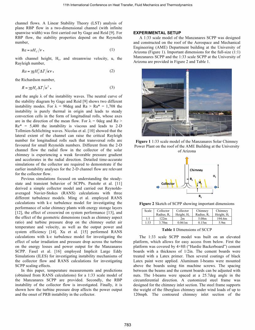
and constructed on the roof of the Aerospace and Mechanical Engineering (AME) Department building at the University of Arizona (Figure 1). Important dimensions for the full-size (1:1) Manzanares SCPP and the 1:33 scale SCPP at the University of Arizona are provided in Figure 2 and Table 1.

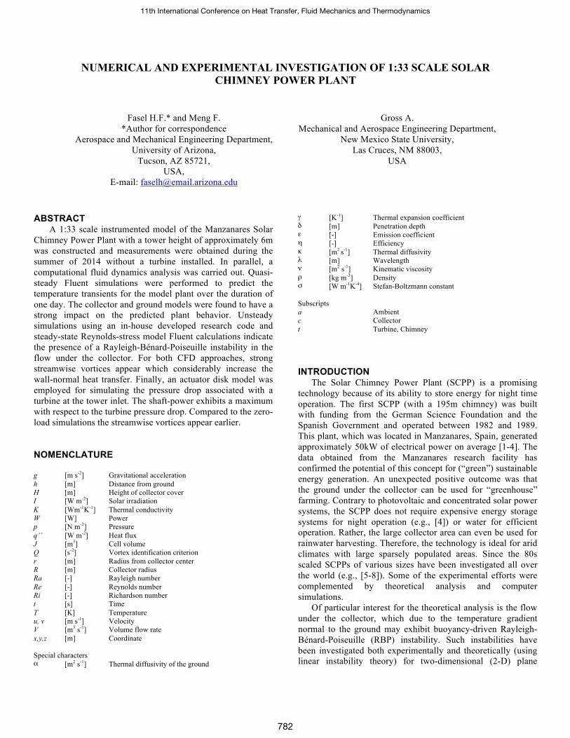
Figure 1 1:33 scale model of the Manzanares Solar Chimney

Power Plant on the roof of the AME Building at the University of Arizona

Figure 2 Sketch of SCPP showing important dimensions

Scale Collector Radius, Rc

Collector Height, Hc

Chimney Radius, Rt

Chimney Height, Ht

1:1 122m 2m 5.08m 194.6m 1:33 3.70m 0.061m 0.15m 5.9m

Table 1 Dimensions of SCCP

The 1:33 scale SCPP model was built on an elevated platform, which allows for easy access from below. First the platform was covered by 4×8ft (“Hardie Backerboard”) cement boards with a thickness of 1/2in. The cement boards were treated with a Latex primer. Then several coatings of black Latex paint were applied. Aluminum I-beams were mounted above the boards using 6in machine screws. The spacing between the beams and the cement boards can be adjusted with nuts. The I-beams were spaced at a 25.7deg angle in the circumferential direction. A customized steel frame was designed for the chimney inlet section. The steel frame supports the weight of the fiberglass chimney under wind loads of up to 120mph. The contoured chimney inlet section of the


783

Manzanares plant (center “spike” and outside contraction) were scaled, fabricated from fiberglass, and mounted inside the steel frame. A fiberglass pipe with 12in inner diameter was lifted to the roof with a crane and anchored on the central steel frame. An aluminum L-beam with 1.5in width was wrapped around the top third of the chimney to alleviate unsteady loads resulting von Karman vortex shedding in high wind situations. Three ¼in stainless steel guy wires were run from the center and the top of the chimney down to the platform. Each set of guy wires is strong enough to withstand a 120mph wind load. If all of the guy wires fail the steel frame at the chimney inlet will still keep the system intact (the entire system was designed with triple redundancy). Rubber U-seals were inserted into the I-beam channels and 14 wedge-shaped polycarbonate greenhouse panels were inserted. At the outer perimeter of the collector aluminum U-beams with rubber U-seals were added. All gaps were sealed with clear silicone. One panel is sealed with tape for easy removal so that the base of the chimney can be accessed easily for making adjustments to the turbine or sensors installed on the bottom of the chimney. To prevent sagging of the panels due to the large unsupported length between the I-beams, supporting aluminum square beams were added on top of the collector.

Figure 3 Thermocouple locations

The solar energy irradiation and absorption by the ground, the ground temperature, the air temperature and velocity in the collector, and the pressure drop across the turbine are some of the quantities that have to be measured in order to define the operating conditions of the SCPP model. For the first series of measurements, which is documented in this paper, J-type (Fe-CuNi) thermocouples were installed inside the collector (Figure 3) and experiments were carried out without a turbine installed. The accuracy of the chosen Omega J-type thermocouples is 0.5K. Thermocouples 1-3 are placed close to the collector inlet at r = 3.3m, thermocouples 4-6 and 7-9 are located at r = 2.67m and r = 2.0m, respectively, and thermocouples 10-12 were installed close to the chimney inlet at r = 1.35m. Thermocouples 1, 4, 7, and 10 provide the temperature of the collector cover. Thermocouples 3, 6, 9, 12 provide the temperature on the top of the absorption layer. Both sets of thermocouples were taped to the respective surfaces. The

remaining thermocouples 2, 5, 8, 11 measure the temperature of the airflow under the collector (between the absorption layer and the collector cover at h = 0.0305m). The ambient air temperature, pressure, wind speed, and normal solar irradiation were obtained from the Atmospheric Technology Division at the University of Arizona once every 5 minutes. Since the weather station at the Physics and Atmospheric Sciences Department is very close to the AME building, where the model is located, it can be assumed that these data provide a sufficiently accurate representation of the ambient state at the model SCPP site.

Figure 4 Labview user interface

The thermocouple analog signals were fed into a National Instruments (NI) SCXI-1303 board, which is designed to minimize errors caused by thermal gradients between the terminals and the cold-junction sensors. The data was then transferred into a NI SCXI-1102 signal amplifier. Finally, a NI SCXI-1600 USB data acquisition and control module was employed for the analog/digital conversion. To reduce signal noise the NI data acquisition electronics were placed directly underneath the platform on which the SCPP model was built. For protecting the electronics from the elements (heat and precipitation) they were placed inside an enclosure, which was equipped with two large PC fans to regulate the internal temperature. Two USB extension kits with 150-foot cable were employed to transfer the data from the NI electronics to a PC in the Computational Fluid Dynamics laboratory in the AME building. Finally, a NI LabVIEW program was developed for conditioning and storing the data and for visualization on a computer screen (Figure 4).

SIMULATION SETUP Reynolds-Averaged Navier-Stokes (RANS) calculations

using ANSYS Fluent and Implicit Large Eddy Simulations (ILES) using an in-house developed compressible Navier-Stokes code [17] were employed for analyzing the 1:33 scale SCPP. A forcing term was added to the vertical momentum equation,

, (4)


784

for modeling the buoyancy effects. Here, J is the cell volume. The dimensionless number, Ri = gHc/v∞

2, which is related to the definition of the Richardson number, results from the non-dimensionalization of the equations.

Axisymmetric ANSYS Fluent calculations with a k-ε turbulence model were employed for investigating the transient behavior of the 1:33 scale SCPP model. For these calculations a simple energy balance model as proposed by Fasel et al. [16] was employed for obtaining the collector ground temperature,

. (5)

Here, I is the direct normal solar irradiation,

is the radiation heat transfer from the

ground, is the radiation heat transfer from the collector (not part of the original model),

is the convective heat transfer from the ground into the air in the collector (which is the usable part), and is the conductive heat transfer into the ground. The emission coefficient was ε = 0.8 and the heat conduction coefficients were Kair = 0.0242W/(mK) and Kground = 0.19W/(mK). A third-order polynomial [18] was assumed for the temperature distribution in the ground,

, (6)

The penetration depth, , scales with the thermal diffusivity of the ground, α = 86.8m2/s (for dry soil), and time t. The collector cover was modeled as an isothermal wall with ambient temperature Ta and was assumed to be 100% transparent with respect to the solar irradiation. The temperature of the air at the collector inlet was set to Ta. The solar irradiation and ambient temperature variation (over the duration of a day-night cycle) were imported from an external file of measured data. To investigate the effect of the turbine on the collector flow, the turbine was modeled as an actuator disk with a preset pressure drop, Δp, across a distance Δx. The turbine shaft power then becomes

, (7)

where ηt represents the turbine efficiency and V is the air volume flow rate through the turbine. According to Gannon and von Backstrom [19] the turbine efficiency can be as high as 80% to 90%.

In addition to the axisymmetric calculations with time-dependent boundary conditions, three-dimensional Fluent calculations with a Reynolds-stress turbulence model were employed for investigating the RBP instability of the collector flow. For these calculations, a constant temperature of 300K was assumed for the collector inflow, the collector top wall,

and the chimney wall and periodicity conditions were employed in the azimuthal direction. The ground temperature was set to 350K.

All Fluent calculations were carried out with the SIMPLE scheme. The convective terms were discretized with a first-order-accurate upwind method because of its superior robustness. The solutions did not change significantly when higher-order-accurate schemes, such as the second order upwind or the QUICK scheme, were employed.

A three-dimensional ILES of the 1:33 scale SCPP was carried out with our compressible in-house developed research code. The computational grid for the ILES consisted of two separate domains with an azimuthal grid opening angle of 15deg for the collector and 45deg for the chimney (an opening angle of 15deg for the chimney domain was found to favor ring-like flow structures). The number of cells was 512 × 64 × 33 for the collector domain and 433 × 64 × 99 for the chimney domain. The maximum near-wall grid resolution in wall units was Δx+

max=76, Δy+max=0.54 and Δz+

max=26 for the collector and Δx+

max=120, Δy+max=1.6 and Δz+

max=10 for the chimney. The Δx+, Δy+, and Δz+ values for the collector are within the resolution requirements for large eddy simulations (50 < Δx+ < 150, Δy+ < 1, and 15 < Δz+ < 40) as recommended by Georgiadis et al. [20]. Since the mean flow properties for the chimney are also reasonably close to the reference Fluent calculations (thus providing the correct collector outflow conditions) it is safe to assume that the present ILES captures the large-scale flow structures in the collector with sufficient accuracy.

For the ILES flow periodicity was enforced in the azimuthal direction and characteristics-based non-reflective boundary conditions were employed at the collector inflow and chimney outflow. A constant temperature of 300K was assumed for the collector inflow, the collector cover, and the chimney wall. The ground temperature was 350K.

MEASUREMENTS AND TRANSIENT SIMULATION In the following, temperature measurements obtained from

the 1:33 scale model for the 10th, 11th, 12th, and 14th of July, 2014 are presented. Based on the measurements for July 14, axisymmetric Fluent calculations (without turbine) were carried out and the predicted collector air temperature was compared with the measured air temperature at a distance of h = 0.0305m from the ground. Thermocouple readings were taken every 5 seconds. The temperature data were then averaged over time intervals of 20min (Figure 5).


785

Figure 5 Chimney inlet temperature, ambient temperature,

solar radiation, and wind speed for the 10th, 11th, 12th, and 14th of July, 2014

The data for the days from July 10 to 12 show that the ambient air temperature and the air temperature under the collector at the chimney inlet rise with increasing solar irradiation and immediately fall when the solar irradiation decreases. This led to the conclusion that the system had very little heat storage capacity. This result is not surprising when considering that the thickness of the cement boards that formed the “ground” was only 1/2in and that the ground was installed on a platform, thus allowing for convective and radiative cooling from underneath. At sunrise on July 14th, the sky was clear and it was sunny from 06:00 to 13:40. Between 10:00 and 14:00 the solar irradiation was above 800W/m2 and the ambient temperature was rising steadily. The chimney inlet airflow temperature quickly reached 50C and then remained almost constant. The observed oscillation of the chimney inflow temperature may be the result of an intermittent cloud obscuration of the collector. At 13:40 the solar irradiation reached a maximum of around 1,100W/m2. At this time the ambient temperature was 33.8C and the chimney inlet temperature was 52.6C. The solar irradiation then remained high for about another hour while the chimney inlet temperature reached a maximum of 57.4C. At this time the temperature difference between the chimney inlet and the ambient was about 21K. Between 14:40 and 16:40 the sky

became very cloudy and the solar irradiation was reduced by over 80% of its peak value. The chimney inlet temperature also fell dramatically. Between 15:20 and 17:00 it was raining and the measured temperature under the collector was below the ambient temperature due to water accumulation under the collector. In addition, wind gusts associated with the convective weather probably led to considerable cooling of the bottom of the platform. Past 17:00 (after the rain) and until sunset the airflow temperature at the chimney inlet did again increase. The ambient temperature on the other hand remained almost constant after the rain. During nighttime, the temperature difference between the chimney inlet and the ambient was negligible.

Figure 6 Measured and computed temperatures for July 14,

2014

A transient (quasi-steady) Fluent simulation was carried out for the conditions of July 14th. The measured time-dependent solar irradiation, ambient air temperature, and temperature at the collector inflow and on top of the collector were prescribed in the simulation. Figure 6 provides the measured chimney inlet flow temperature (location 11), the measured ground temperature (location 12), and the measured collector cover temperature (location 10) as well as the respective temperatures for the same locations as obtained from the simulation. Since the collector cover temperature in the simulation was preset to be the same as the measured ambient temperature, the ambient temperature in Figure 6 is also the cover temperature in the simulation. In the simulation the increase in ground temperature and chimney inlet airflow temperature is approximately proportional to the increase in solar irradiation.

The measured ground temperature reaches a peak value slightly above 60C at 10:40 and then remains around 60C. In the simulation the ground temperature climbs somewhat faster and keeps increasing beyond 10:40. At about 14:00 when the measured solar irradiation reaches its peak value the predicted ground temperature hits a maximum of 75C, which is 15K above the measured value. Most likely, this difference can be traced back to the models that were employed for the ground and collector. Another possibility is that the thermocouples in the experiment were placed too far from the ground, which would result in lower temperature readings. These and other possibilities for the observed discrepancies will be explored in


786

the future. The predicted air temperature at the chimney inlet approximately follows the measured air temperature at the chimney inlet. In the simulation the collector cover temperature was identical to the ambient temperature. The collector was simplified as a thin transparent layer without heat storage capacity and with 100% transparency for the solar irradiation. In the experiment, the temperature of the collector panels was increasing slightly (not shown) because they absorbed part of the solar irradiation. Likely the panels also reflected part of the incoming solar irradiation. This “loss” of solar irradiation provides another reason why the measured ground temperature was lower than the simulated ground temperature.

Figure 7 Temperature as a function of radial position at 9:00

and 14:00

In Figure 7 the temperature (ground and air temperature) are presented for 9:00 and 14:00 for several radial locations. At both times, compared to the experiment, the ground temperature in the simulation is lower near the collector inflow and then rises more quickly towards the chimney inlet. This may again be an indication that compared to the experiment more solar irradiation reached the ground in the simulation. Interestingly, the measured air temperature in the simulation is lower than in the experiment. In the simulation the air at the collector inflow was assumed to be at ambient temperature. In the experiment, the black painted absorption layer (cement boards) reached farther out and most likely preheated the air before it entered the collector. Compared to the experiment, the air temperature in the collector rises more quickly in the

simulation. Since the ground temperature is higher in the simulation this would be expected.

In summary, the simulation approximately captures the physics and models the system performance of the model SCPP. The ground and collector models and the instrumentation of the experiment will be improved in order to better understand the reasons for the discrepancies between simulation results and the measurements. For example, pyranometers will be added to measure the broadband solar irradiation at different locations inside the collector.

At 14:00 the ground temperature in the collector was approximately 63C or 336K and thus close to the assumed ground temperature of 350K in the following investigations with fixed ground temperature. Therefore, these simulations where the RBP instability in the collector and the effect of a turbine pressure drop were investigated are relevant for the model SCPP experiment.

THREE-DIMENSIONAL SIMULATIONS Both an ILES using the in-house developed research code

and a three-dimensional RANS calculation with a Reynolds-Stress Model (RSM) using the Fluent code were carried out for the model SCCP. The inflow velocity for the ILES was set to 0.15m/s resulting in a Reynolds number at the collector inflow of Re=vin×Hc/ν=610. These values approximately match the corresponding values of the Fluent calculation where the inflow velocity was not specified. For both simulations the ground temperature was set to 350K and the collector cover temperature was set to 300K. These conditions are characteristic for the model operating conditions during the afternoon. The Reynolds number (based on Hc) for the flow under the collector for r/Rc > 0.12 is less than the critical Reynolds number for the least stable viscous mode, i.e. Re* = 5,400, for a plane channel flow [9]. Disregarding the differences between the present case (accelerated radial flow with favorable pressure gradient; finite azimuthal extent of domain) and the plane channel flow analysis, a viscous instability can be expected for r=Rc < 0.12.

Flow visualizations of the instantaneous and the time-averaged data from the ILES are provided in Figure 8. Shown are iso-surfaces of the Q-vortex identification criterion [21], which indicates areas where rotation dominates strain. The flow in the collector evolves from an initial state of fully developed laminar channel flow. Two-dimensional transverse rolls develop periodically near the collector inflow, presumably as a consequence of a RBP instability. Because of the very low Reynolds number at the collector inlet these structures are likely not resulting from a viscous instability but rather may be attributed to a buoyancy-driven instability. As suggested by the linear stability theory analysis by Fujimura and Kelly [22], transverse rolls can develop for small Reynolds numbers when the Rayleigh number is greater than the critical Rayleigh number, i.e. Ra > 1,708 (the Rayleigh for the present simulation is about Ra = 177,800). The viscosity of the air in the collector is increasing near the ground (the ground is hotter than the collector cover) and the flow is accelerating in the radial


787

direction. Both factors likely have a stabilizing effect on the naturally occurring instabilities.

Figure 8 Instantaneous (top) and time-averaged (bottom) iso-

surfaces of Q=0.01 colored by temperature (300<T<350K) obtained from ILES

Figure 9 Iso-contours of radial vorticity at collector mid-height

(h = 0.0325m) obtained from RANS calculation

Figure 10 Temperature iso-contours at collector inflow (time and spanwise average). ILES (top), Fluent RSM calculation

(bottom)

Near r = 3.1m the transverse rolls become wavy in the azimuthal direction and longitudinal rolls begin to develop. The number of longitudinal rolls per 15deg segment is decreasing in the streamwise direction. Because the transverse rolls are traveling, they do not contribute to the time-average (Figure 8). According to Gage and Reid [9], longitudinal rolls should always show up first. At this point, it is not fully understood why transverse rolls appear near the collector inflow. A similar behavior was observed by, e.g. Nicolas et al. [10] for a much lower Reynolds number. The longitudinal rolls also showed up in the Fluent RSM calculation. Iso-contours of the radial vorticity indicate that longitudinal rolls develop near r = 2.5m (Figure 9). At this location six longitudinal rolls were counted per 15deg segment. In the downstream direction the longitudinal rolls merged and the number of structures per

segment decreased according to the ILES simulation. The appearance of the longitudinal rolls leads to strong convective mixing in the wall-normal direction. As a result, the hot air near the ground is very effectively spread across the entire collector height (Figure 10).

Instantaneous flow visualizations at the chimney inlet and outlet obtained from the ILES indicate a fully turbulent flow (Figure 11). The azimuthal domain extent employed for the chimney was 45deg. This domain extent reduces the bias regarding azimuthal structures (ring-like flow structures) seen in earlier simulations where the domain extent for the chimney was only 15deg.

Figure 11 Instantaneous iso-surfaces of Q=0.1 colored by

temperature at chimney inflow and outflow

Figure 12 Collector velocity and temperature profiles (ILES)

Figure 13 Collector velocity and temperature profiles (RANS)

Wall-normal profiles of the radial velocity and temperature (time- and spanwise-averaged data) for the flow under the collector are shown in Figures 12 & 13. In the ILES a parabolic velocity profile was prescribed at the collector inflow, while in the Fluent RSM calculation a top-hat velocity profile was specified. As a result at r = 3.3m the RANS profile is less full. Other than that the match between the profiles obtained from the ILES and the RANS calculation is remarkably good. The


788

profiles illustrate an accelerating asymmetric flow with temperature gradient.

SIMULATIONS WITH TURBINE PRESSURE DROP Additional axisymmetric Fluent RANS calculations were

carried out to investigate the effect of a turbine pressure drop. The turbine was modeled by use of an “actuator disk”. Different pressure drops across the actuator disk, Δp = 1.0, 2.0, 3.0 and 3.5Pa, were considered. In Figure 14 a comparison between a calculation without turbine and with turbine (pressure drop 3Pa) is provided. With the turbine, as expected, the static pressure at the chimney inlet is increased and the axial velocity is reduced.

Figure 14 Contours of static pressure and axial (updraft)

velocity for zero-load (left) and Δp = 3Pa turbine pressure drop (right)

Figure 15 Collector velocity and temperature profiles for Δp =

3Pa (RANS)

Figure 16 Temperature profiles at collector outlet

Velocity and temperature profiles are provided in Figure 15. Compared to the case with zero turbine load (Figure 13) the radial velocity is reduced by a factor three and the temperature is increased. In particular, with the turbine the temperature profiles for r = 1.76m and 0.98m are almost identical indicating “saturation” while for the case with zero load the air temperature is still increasing for these two stations.

The turbine pressure drop reduces the air velocity in the chimney. As a result the residence time of the air in the collector is increased thus allowing for a larger transfer of thermal energy from the ground into the air. As a result the temperature at the collector outlet rises with increasing turbine pressure drop (Figure 16). The maximum difference between the temperature profiles for Δp = 0Pa and Δp = 3.5Pa is 3.7K.

Since the turbine pressure drop also leads to a reduction of the total flow rate an optimum for the output power exists. The turbine power output was computed assuming a turbine efficiency of 100%. Volume flow rate and output power are plotted in Figure 17. The volume flow rate decreases almost inversely proportional to the turbine pressure drop. The maximum output power (0.26W) is achieved for Δp = 3.0Pa. The maximum potential pressure drop in the system is around 3.8Pa. For both Δp = 0 and Δp ≈ 3.8Pa the output power is zero.

Figure 17 Volume flow rate and shaft power as function of

turbine pressure drop

Figure 18 Iso-contours of radial vorticity at h = 0.0305m (top)

and temperature (spanwise average) for Δp = 3.0Pa

Contours of the radial vorticity component for Δp = 3.0Pa are provided in Figure 18. Compared to the case with zero load (Figure 9), the longitudinal rolls appear earlier, i.e., at r = 3.1m. Because the velocity is lower compared to the case with zero-load, the Reynolds number is lower. The Rayleigh number, on the other hand, is close to the Rayleigh number for the zero-load case because the temperature gradient is larger. The


789

number of longitudinal rolls counted across the 15deg segment at the onset of the instability is eight and thus larger than for the zero-load case. As for the zero-load case, the longitudinal rolls merge in the streamwise direction. The earlier appearance of the longitudinal rolls and the associated wall-normal convective mixing provides another mechanism for increasing the thermal energy transfer from the ground to the flow under the collector (Figure 18).

CONCLUSION A 1:33 scale model of the Manzanares solar chimney power

plant was constructed on the roof of the Aerospace and Mechanical Engineering building at the University of Arizona. The model was instrumented with temperature probes and measurements were carried out over the duration of several days. Transient (quasi-steady) Fluent calculations, where the inflow and ground temperature were prescribed according to the measurements, showed qualitative agreement of some aspects of the flow and systematic disagreement in others. This clearly indicates that an improvement of the ground and collector cover models is required in order to accurately predict the flow behavior and performance of SCPPs.

Results from time-resolved simulations exhibited the presence of traveling transverse rolls near the collector inflow for the zero-load (no turbine) conditions. About one-third into the collector, steady streamwise rolls appeared. The existence of the streamwise structures was confirmed by a comparison with a RANS calculation (FLUENT) using a Reynolds-stress turbulence model. The longitudinal rolls were found to greatly increase the wall-normal heat transfer in the flow under the collector.

Finally, Fluent calculations with actuator disk model for the turbine were carried out. The pressure drop across the turbine led to a reduction of the volume flow rate and an increase of the air temperature at the collector outlet (or chimney inlet). The power output showed a maximum with respect to the pressure drop. For the maximum power condition the longitudinal structures in the collector appeared earlier compared to the zero-load condition.

The Reynolds and Rayleigh numbers for the Manzanares plant are considerably higher than for the 1:33 scale model. Nevertheless, the observed strong instabilities for the 1:33 scale model suggest that coherent structures embedded in a turbulent flow can also be expected for large-scale plants. Therefore the instabilities of the collector should be investigated for full-size solar chimney plants.

ACKNOWLEDGEMENT This research was funded by the University of Arizona 1885

Society and supported by the University of Arizona TRIF-funded Water, Environmental and Energy Solutions initiative co-managed by the Water Sustainability Program, Institute of the Environment, and Renewable Energy Network. The authors would like to thank Schlaich Bergermann & Partner for providing the geometric details of the original Manzanares SCPP.

REFERENCES [1] Haaf, W., Friedrich, K., Mayr, G., and Schlaich, J., Solar

chimneys, part I: principle and construction of the pilot plant in Manzanares. International Journal of Sustainable Energy, Vol. 2, 1983, pp. 3–20

[2] Haaf, W., Solar chimneys, part II: preliminary test results from the Manzanares pilot plant, International Journal of Solar Energy, Vol. 2, 1984, pp. 141–161

[3] Schlaich, J., The Solar Chimney – Electricity from the Sun, Eds. F.W. Schubert and J. Schlaich, Edition Axel Menges, Deutsche Verlagsanstalt, Stuttgart, C. Maurer, Geislingen, Germany, 1995

[4] Schlaich, J., Bergermann, R., Schiel, W., and Weinerbe, G., Design of commercial solar updraft tower systems-utilization of solar induced convective flows for power generation, Journal of Solar Energy Engineering, Vol. 127, 2005, pp. 117-124

[5] Pretorius, J.P., and Kroger, D.G., Solar Chimney Power Plant Performance, Journal of Solar Energy Engineering, Vol. 128, 2006, pp. 302–311

[6] Zhou, X., Yang, J., Xiao, B., and Hou, G., Simulation of a pilot solar chimney thermal power generating equipment, Renewable Energy, Vol. 32, 2007, pp. 1637–1644

[7] Maia, C.B., Ferreira, A.G., Valle, R.M., and Cortez, M.F.B., Theoretical evaluation of the influence of geometric parameters and materials on the behavior of the air-flow in a solar chimney, Computers and Fluids, Vol. 38, 2009, pp. 625–636

[8] Larbi, S., Bouhdjar, A., and Chergui, T., Performance analysis of a solar chimney power plant in the southwestern region of Algeria, Renewable and Sustainable Energy Reviews, Vol. 14, 2010, pp. 470–477

[9] Gage, K.S., and Reid, W.H., The stability of thermally Stratified Plane Poiseuille Flow, Journal of Fluid Mechanics, Vol. 33, 1968, pp. 21-32

[10] Nicolas, X., Luijkx, J.-M., and Platten, J.-K., Linear stability of mixed convection flows in horizontal rectangular channels of finite transversal extension heated from below, International Journal of Heat and Mass Transfer, Vol. 43, 2000, pp. 589-610

[11] Pastohr, H., Kornadt, O., and Gurlebeck, K., Numerical and analytical calculations of the temperature and flow field in the upwind power plant. International Journal of Energy Research, Vol. 28, 2004, pp. 495–510

[12] Ming, T.Z., Liu, W., Pan, Y., and Xu, G.L., Numerical analysis of flow and heat transfer characteristics in solar chimney power plants with energy storage layer, Energy Conversion and Management, Vol. 49, 2008, pp. 2872–2879

[13] Ming, T., Wang, X., de Richter, R.K., Liu, W., Wu, T., and Pan, Y., Numerical analysis on the influence of ambient crosswind on the performance of solar updraft power plant system, Renewable and Sustainable Energy Reviews, Vol. 16, 2012, pp. 5567–5583

[14] Ming, T., de Richter, R.K., Meng, F., Pan, Y., and Liu, W., Chimney shape numerical study for solar chimney power generating systems, International Journal of Energy Research, Vol. 37, 2013, pp. 310–322

[15] Xu, G., Ming, T., Pan, Y., Meng, F., and Zhou, C., Numerical analysis on the performance of solar chimney power plant system, Energy Conversion and Management, Vol. 52, 2011, pp. 876–883

[16] Fasel, H.F., Meng, F., Shams, E., and Gross, A., CFD Analysis for Solar Chimney Power Plants, Solar Energy, Vol. 98, 2013, pp. 12–22

[17] Gross, A., and Fasel, H.F., High-Order Accurate Numerical Method for Complex Flows, AIAA Journal, Vol. 46, 2008, pp. 204-214


790

[18] Ozisik, M. N., Heat Conduction, John Wiley, New York, 1993 [19] Gannon, A.J., and von Backstrom, T.W., Solar chimney turbine

performance, Journal of Solar Energy Engineering, Vol. 125, 2003, pp. 101-106

[20] Georgiadis, N.J., Rizzetta, D.P., and Fureby, C., Large-Eddy Simulation: Current Capabilities, Recommended Practices, and Future Research, AIAA Journal, Vol. 48, 2010, pp. 1772-1784

[21] Hunt, J.C.R., Wray, A.A., and Moin, P., Eddies, stream, and convergence zones in turbulent flows, Report CTR-S88, Center for Turbulence Research, Stanford, CA, 1988

[22] Fujimura, K., and Kelly, R.E., Interaction between Longitudinal Convection Rolls and Transverse Waves in Unstably Stratified Plane Poiseuille Flow, Physics of Fluids, Vol. 7, 1995, pp. 68-79


791

NUMERICAL AND EXPERIMENTAL INVESTIGATION OF 1:33 …

Documents

Transcript of NUMERICAL AND EXPERIMENTAL INVESTIGATION OF 1:33 …