NUMERICAL ANALYSIS Numerical solutions of algebraic ...mathskthm.6te.net/Numerical Analysis...

NET/SET Preparation Numerical Analysis By S. M. CHINCHOLE

1

NUMERICAL ANALYSIS

Numerical solutions of algebraic equations, Method of iteration and

Newton-Raphson method, Rate of convergence, Solution of systems

of linear algebraic equations using Gauss elimination and Gauss-

Seidel methods, Finite differences, Lagrange, Hermite and spline

interpolation, Numerical differentiation and integration, Numerical

solutions of ODEs using Picard, Euler, modified Euler and Runge-

Kutta methods.

Numerical Solutions of Algebraic Equations

If the goal is to solve , then the function can be plotted in a way that the

intersection of with the -axis is visible and the root is found. We should have a rather

good idea as of where to look for the root. sometimes it is easier to verify that the function

is continuous (which hopefully it is) in which case all that we need is to find a point in

which , and a point , in which . The continuity will then guarantee (due

to the intermediate value theorem) that there exists a point between and for which

.

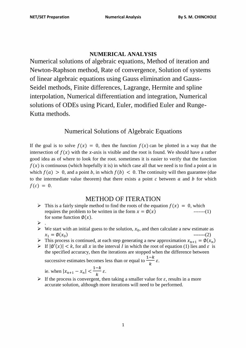
METHOD OF ITERATION This is a fairly simple method to find the roots of the equation , which

requires the problem to be written in the form -------(1)

for some function . .

We start with an initial guess to the solution, , and then calculate a new estimate as

-------(2)

This process is continued, at each step generating a new approximation If | | for all in the interval in which the root of equation (1) lies and is

the specified accuracy, then the iterations are stopped when the difference between

successive estimates becomes less than or equal to

.

ie. when | |

.

If the process is convergent, then taking a smaller value for , results in a more

accurate solution, although more iterations will need to be performed.


2

Y

X

Example 1: Find a real root of the equation -----(1)

(which has the exact solution ).

We first need to write the equation in the form , and then there is more than

one way of doing this.

One way is to write the equation as ⁄ so

⁄

If we start an initial guess of , then above iterative method then gives:

Iteration 1 2 3 4 5 6 7 8 9 10 11

2.5 3.12 3.49 3.71 3.83 3.91 3.95 3.97 3.98 3.99 3.99

3.12 3.49 3.71 3.83 3.91 3.95 3.97 3.98 3.99 3.99 4.00

Example 2: Find a real root of the equation on the interval [ ] with an

accuracy of .

Consider the equation -----(1)

One way is to write the equation as

√ -----(2)

Thus

√ and

⁄

Also | |[ ] |

⁄ |

(

⁄ )

⁄ =

√

Hence | |

i.e. when the absolute value of the difference does not exceed , the required

accuracy will be achieved and then iteration can be terminated.


3

Starting with , we obtain the following table

n √

√

0 0.75 1.3228756 0.7559289

1 0.7559289 1.3251146 0.7546517

2 0.7546517 1.3246326 0.7549263

At this stage, we find that | |

which is less than . The iteration is therefore terminated and the root to the

required accuracy is .

Example 3: Find the root of the equation correct to three decimal places.

Consider the equation -----(1)

We rewrite this equation as

-----(2)

Thus

and

and hence | |

Hence | |

Hence the iteration method can be applied to the equation (1) and we start with

⁄ . The successive iterates are , , ,

, , , ,

Hence we take the solution as 1.524 correct to three decimal places.

NEWTON-RAPHSON METHOD This method is also useful to solve the equation .

Let be an approximate root of and let be the correct root so

that . Then by Taylor’s series, we obtain

Neglecting the second and higher-order derivatives, we have

, which gives

A better approximation than is therefore given by , where

Successive approximations are given by , , , ..., , where

which is the Newton- Raphson formula.

Example 4: Use the Newton-Raphson method to find a root of the equation

.

Here and . Hence

gives

-----(1)

Choosing , we obtain and . Putting the value

and then putting the values of and in equation (1), we get


4

(

)

Now,

,

and .

Hence by putting the value and then putting the values of and in

equation (1), we get

(

)

Example 5: Find a root of the equation .

Here and .

The iteration formula therefore becomes

With , the successive iterates are given below

0 3.1416 -1.0 2.8233

1 2.8233 -0.0662 2.7986

2 2.7986 -0.0006 2.7984

3 2.7984 0.0 2.7984

Example 6: Find a real root of the equation , using the Newton-Raphson method.

Here and .

Let . Then and . Putting the value and then

putting the values of and in equation (1), we get

(

)

Now , and ,

So that

.

Proceeding in this way, we obtain and .

RATE OF CONVERGENCE The sequences ⁄ , ⁄ , ⁄ , and ⁄ all converge

to .

How fast?

⁄ , ⁄ , ⁄ , and ⁄ is true, but doesn’t really convey

how slow , or how fast . We use functions like these, and more

generally ⁄ and ⁄ as yardsticks (or benchmarks) with which to compare the

speed of convergence of algorithms.

In our context, we are usually trying to compute better and better approximations

to some value , and we want to know how fast the error | | is converging

toward . It is nice to be able to say (our approximations will eventually be

close to the answer), but will it take a second or a week? In the example above

, but .


5

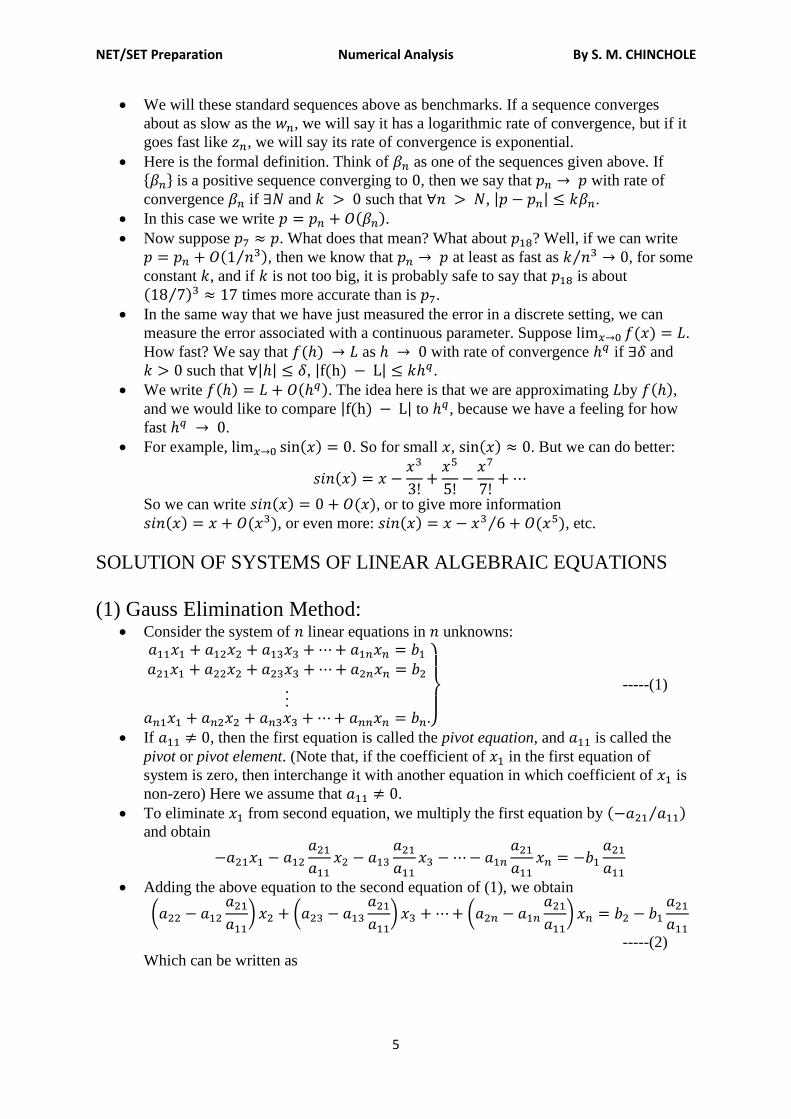
We will these standard sequences above as benchmarks. If a sequence converges

about as slow as the , we will say it has a logarithmic rate of convergence, but if it

goes fast like , we will say its rate of convergence is exponential.

Here is the formal definition. Think of as one of the sequences given above. If { } is a positive sequence converging to , then we say that with rate of

convergence if and such that , | | .

In this case we write . Now suppose . What does that mean? What about ? Well, if we can write

⁄ , then we know that at least as fast as ⁄ , for some

constant , and if is not too big, it is probably safe to say that is about

⁄ times more accurate than is .

In the same way that we have just measured the error in a discrete setting, we can

measure the error associated with a continuous parameter. Suppose .

How fast? We say that as with rate of convergence if and

such that | | , | | .

We write . The idea here is that we are approximating by , and we would like to compare | | to , because we have a feeling for how

fast .

For example, . So for small , . But we can do better:

So we can write , or to give more information

, or even more: ⁄ , etc.

SOLUTION OF SYSTEMS OF LINEAR ALGEBRAIC EQUATIONS

(1) Gauss Elimination Method: Consider the system of linear equations in unknowns:

}

-----(1)

If , then the first equation is called the pivot equation, and is called the

pivot or pivot element. (Note that, if the coefficient of in the first equation of

system is zero, then interchange it with another equation in which coefficient of is

non-zero) Here we assume that .

To eliminate from second equation, we multiply the first equation by ⁄ and obtain

Adding the above equation to the second equation of (1), we obtain

(

) (

) (

)

-----(2)

Which can be written as


6

,

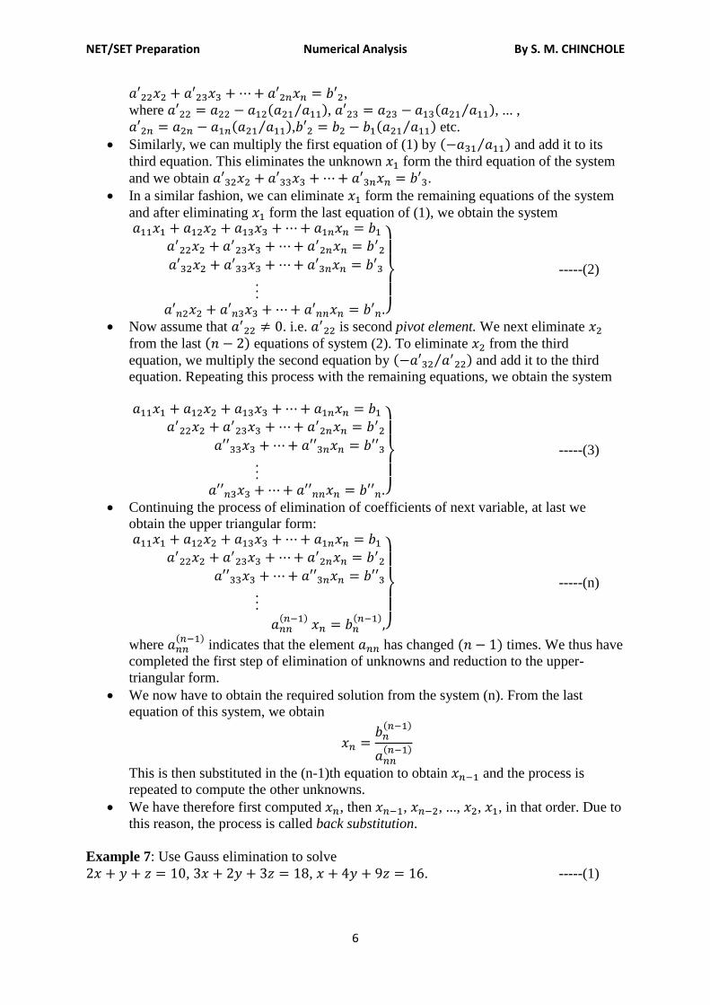
where ⁄ , ⁄ , ... , ⁄ , ⁄ etc.

Similarly, we can multiply the first equation of (1) by ⁄ and add it to its

third equation. This eliminates the unknown form the third equation of the system

and we obtain .

In a similar fashion, we can eliminate form the remaining equations of the system

and after eliminating form the last equation of (1), we obtain the system

}

-----(2)

Now assume that . i.e.

is second pivot element. We next eliminate

from the last equations of system (2). To eliminate from the third

equation, we multiply the second equation by ⁄ and add it to the third

equation. Repeating this process with the remaining equations, we obtain the system

}

-----(3)

Continuing the process of elimination of coefficients of next variable, at last we

obtain the upper triangular form:

}

-----(n)

where

indicates that the element has changed times. We thus have

completed the first step of elimination of unknowns and reduction to the upper-

triangular form.

We now have to obtain the required solution from the system (n). From the last

equation of this system, we obtain

This is then substituted in the (n-1)th equation to obtain and the process is

repeated to compute the other unknowns.

We have therefore first computed , then , , ..., , , in that order. Due to

this reason, the process is called back substitution.

Example 7: Use Gauss elimination to solve

, , . -----(1)


7

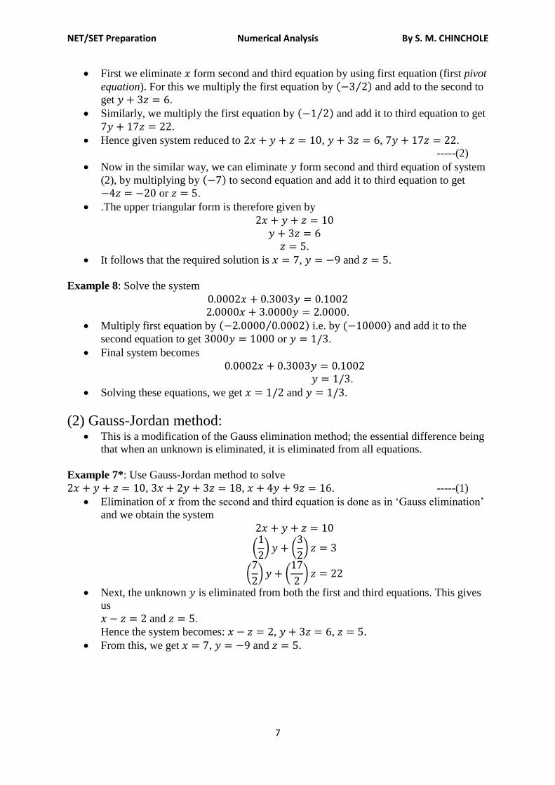
First we eliminate form second and third equation by using first equation (first pivot

equation). For this we multiply the first equation by ⁄ and add to the second to

get .

Similarly, we multiply the first equation by ⁄ and add it to third equation to get

.

Hence given system reduced to , , .

-----(2)

Now in the similar way, we can eliminate form second and third equation of system

(2), by multiplying by to second equation and add it to third equation to get

or .

.The upper triangular form is therefore given by

.

It follows that the required solution is , and .

Example 8: Solve the system

.

Multiply first equation by ⁄ i.e. by and add it to the

second equation to get or .

Final system becomes

.

Solving these equations, we get and .

(2) Gauss-Jordan method: This is a modification of the Gauss elimination method; the essential difference being

that when an unknown is eliminated, it is eliminated from all equations.

Example 7*: Use Gauss-Jordan method to solve

, , . -----(1)

Elimination of from the second and third equation is done as in ‘Gauss elimination’

and we obtain the system

(

) (

)

(

) (

)

Next, the unknown is eliminated from both the first and third equations. This gives

us

and .

Hence the system becomes: , , .

From this, we get , and .


8

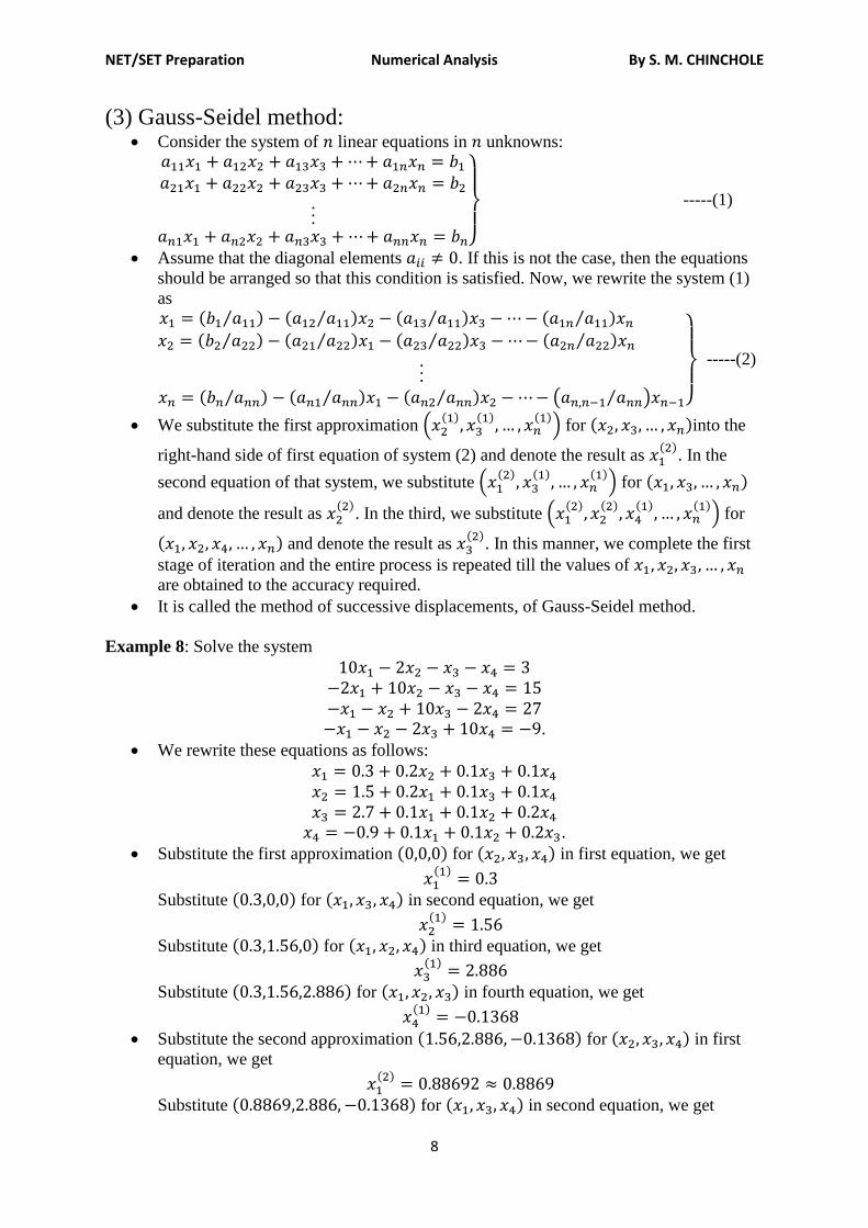
(3) Gauss-Seidel method: Consider the system of linear equations in unknowns:

}

-----(1)

Assume that the diagonal elements . If this is not the case, then the equations

should be arranged so that this condition is satisfied. Now, we rewrite the system (1)

as

⁄ ⁄ ⁄ ⁄

⁄ ⁄ ⁄ ⁄

⁄ ⁄ ⁄ ( ⁄ ) }

-----(2)

We substitute the first approximation (

) for into the

right-hand side of first equation of system (2) and denote the result as

. In the

second equation of that system, we substitute (

) for

and denote the result as

. In the third, we substitute (

) for

and denote the result as

. In this manner, we complete the first

stage of iteration and the entire process is repeated till the values of

are obtained to the accuracy required.

It is called the method of successive displacements, of Gauss-Seidel method.

Example 8: Solve the system

.

We rewrite these equations as follows:

.

Substitute the first approximation for in first equation, we get

Substitute for in second equation, we get

Substitute for in third equation, we get

Substitute for in fourth equation, we get

Substitute the second approximation for in first

equation, we get

Substitute for in second equation, we get


9

Substitute for in third equation, we get

Substitute for in fourth equation, we get

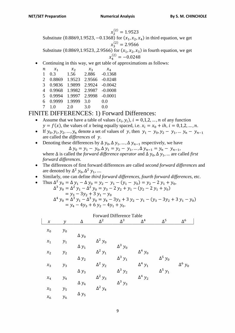
Continuing in this way, we get table of approximations as follows:

1 0.3 1.56 2.886 -0.1368

2 0.8869 1.9523 2.9566 -0.0248

3 0.9836 1.9899 2.9924 -0.0042

4 0.9968 1.9982 2.9987 -0.0008

5 0.9994 1.9997 2.9998 -0.0001

6 0.9999 1.9999 3.0 0.0

7 1.0 2.0 3.0 0.0

FINITE DIFFERENCES: 1) Forward Differences: Assume that we have a table of values , of any function

, the values of being equally spaced, i.e. , .

If denote a set of values of , then

are called the differences of .

Denoting these differences by respectively, we have

,

where is called the forward difference operator and are called first

forward differences.

The differences of first forward differences are called second forward differences and

are denoted by .

Similarly, one can define third forward differences, fourth forward differences, etc.

Thus

.

Forward Difference Table


10

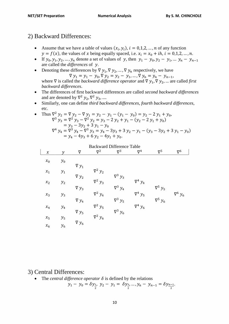
2) Backward Differences:

Assume that we have a table of values , of any function

, the values of being equally spaced, i.e. , .

If denote a set of values of , then

are called the differences of .

Denoting these differences by respectively, we have

,

where is called the backward difference operator and are called first

backward differences.

The differences of first backward differences are called second backward differences

and are denoted by .

Similarly, one can define third backward differences, fourth backward differences,

etc.

Thus

.

Backward Difference Table

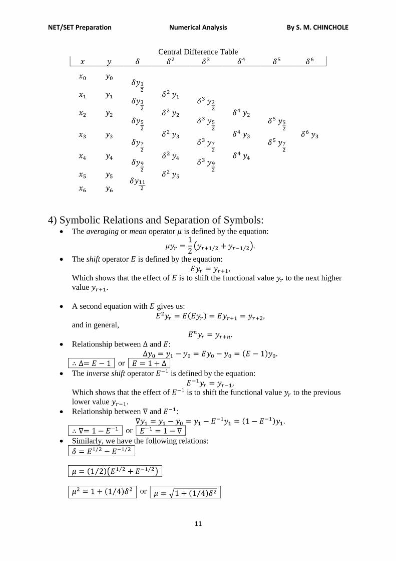
3) Central Differences: The central difference operator is defined by the relations

.


11

Central Difference Table

4) Symbolic Relations and Separation of Symbols: The averaging or mean operator is defined by the equation:

( ⁄ ⁄ )

The shift operator is defined by the equation:

Which shows that the effect of is to shift the functional value to the next higher

value .

A second equation with gives us:

and in general,

Relationship between and :

or

The inverse shift operator is defined by the equation:

Which shows that the effect of is to shift the functional value to the previous

lower value .

Relationship between and :

or

Similarly, we have the following relations:

⁄ ⁄

⁄ ( ⁄ ⁄ )

⁄ or √ ⁄


12

⁄

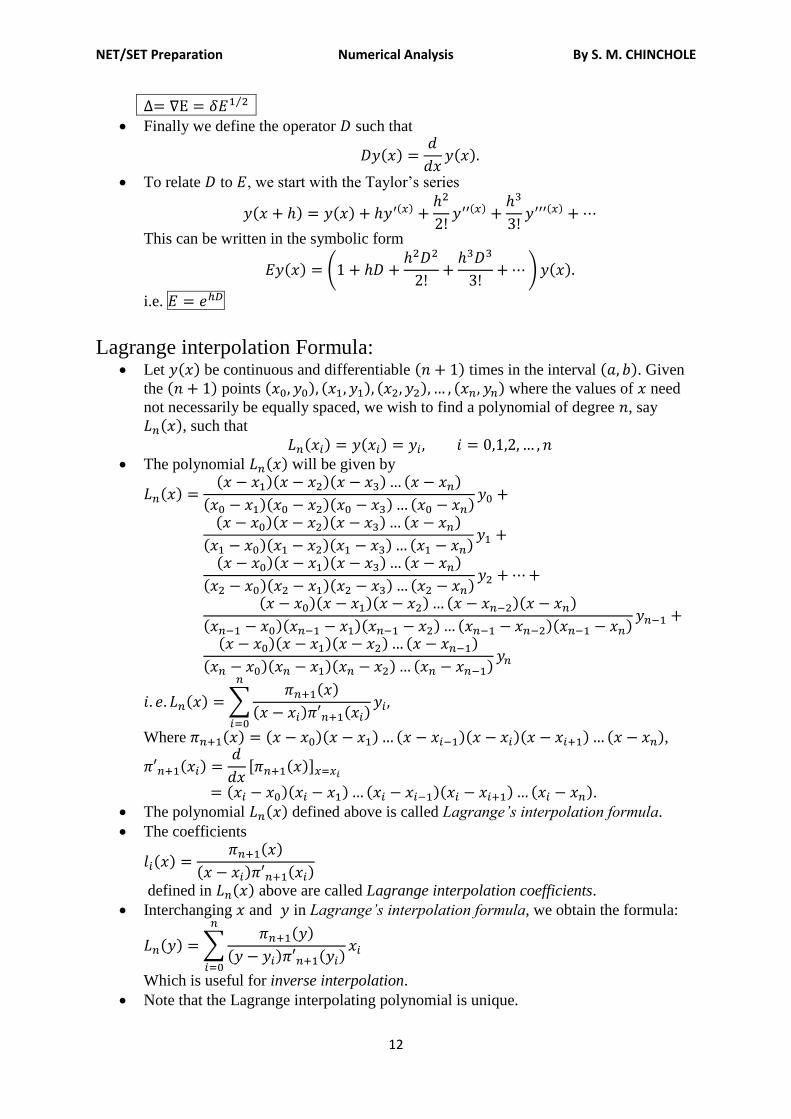
Finally we define the operator such that

To relate to , we start with the Taylor’s series

This can be written in the symbolic form

(

)

i.e.

Lagrange interpolation Formula: Let be continuous and differentiable times in the interval . Given

the points where the values of need

not necessarily be equally spaced, we wish to find a polynomial of degree , say

, such that

The polynomial will be given by

∑

Where ,

[ ]

. The polynomial defined above is called Lagrange’s interpolation formula.

The coefficients

defined in above are called Lagrange interpolation coefficients.

Interchanging and in Lagrange’s interpolation formula, we obtain the formula:

∑

Which is useful for inverse interpolation.

Note that the Lagrange interpolating polynomial is unique.


13

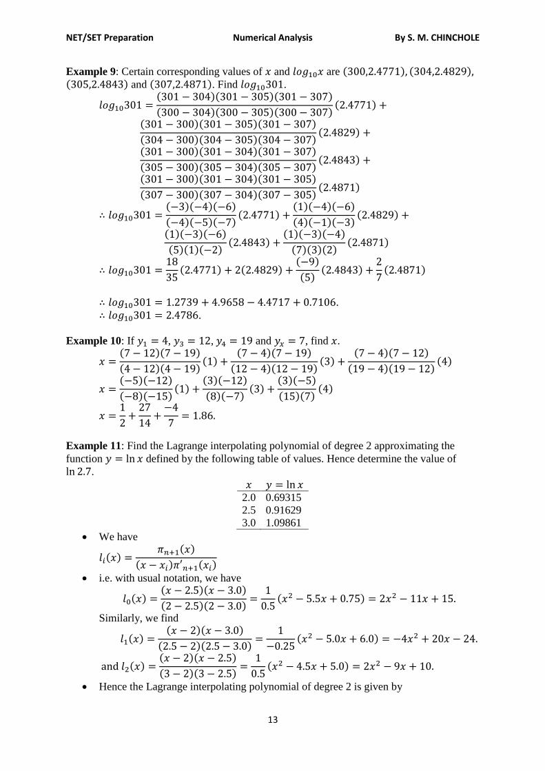
Example 9: Certain corresponding values of and are and . Find .

.

.

Example 10: If , , and , find .

Example 11: Find the Lagrange interpolating polynomial of degree 2 approximating the

function defined by the following table of values. Hence determine the value of

.

2.0 0.69315

2.5 0.91629

3.0 1.09861

We have

i.e. with usual notation, we have

Similarly, we find

Hence the Lagrange interpolating polynomial of degree 2 is given by


14

∑

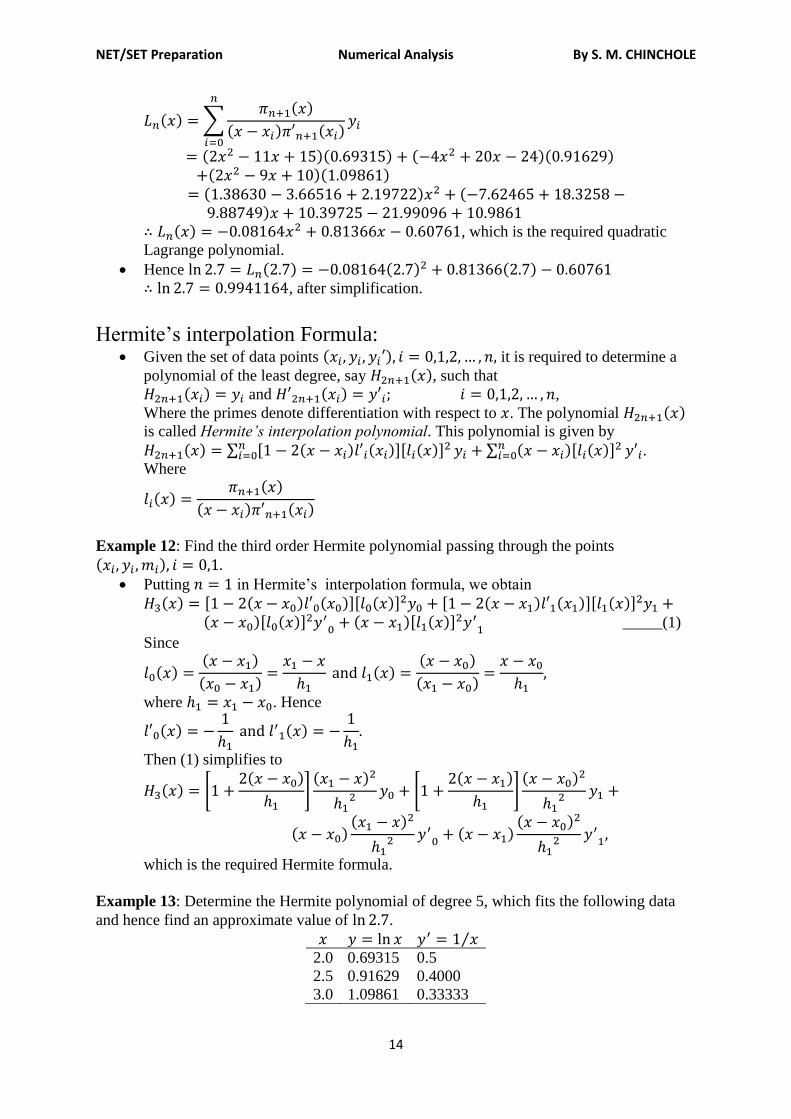
, which is the required quadratic

Lagrange polynomial.

Hence

, after simplification.

Hermite’s interpolation Formula: Given the set of data points it is required to determine a

polynomial of the least degree, say , such that

and ,

Where the primes denote differentiation with respect to . The polynomial is called Hermite’s interpolation polynomial. This polynomial is given by

∑ [ ][ ]

∑ [ ]

. Where

Example 12: Find the third order Hermite polynomial passing through the points

Putting in Hermite’s interpolation formula, we obtain

[ ][ ] [ ][ ]

[ ]

[ ]

_____(1)

Since

where . Hence

Then (1) simplifies to

*

+

*

+

which is the required Hermite formula.

Example 13: Determine the Hermite polynomial of degree 5, which fits the following data

and hence find an approximate value of .

⁄

2.0 0.69315 0.5

2.5 0.91629 0.4000

3.0 1.09861 0.33333


15

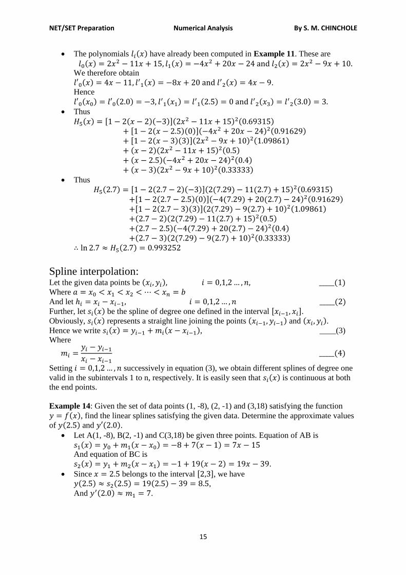
The polynomials have already been computed in Example 11. These are

We therefore obtain

.

Hence

Thus

[ ] [ ] [ ]

Thus

[ ]

[ ]

[ ]

Spline interpolation: Let the given data points be Where

And let Further, let be the spline of degree one defined in the interval [ ]. Obviously, represents a straight line joining the points and . Hence we write , ____(3)

Where

Setting successively in equation (3), we obtain different splines of degree one

valid in the subintervals 1 to n, respectively. It is easily seen that is continuous at both

the end points.

Example 14: Given the set of data points (1, -8), (2, -1) and (3,18) satisfying the function

, find the linear splines satisfying the given data. Determine the approximate values

of and . Let A(1, -8), B(2, -1) and C(3,18) be given three points. Equation of AB is

And equation of BC is

.

Since belongs to the interval [ ], we have

,

And .


16

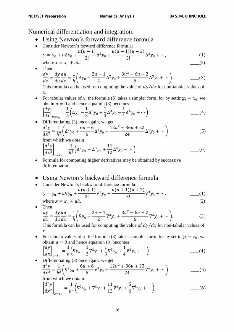
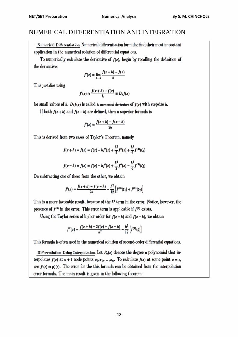
Numerical differentiation and integration:

Using Newton’s forward difference formula Consider Newton’s forward difference formula:

where . ____(2)

Then

(

)

This formula can be used for computing the value of ⁄ for non-tabular values of

.

For tabular values of , the formula (3) takes a simpler form, for by setting , we

obtain and hence equation (3) becomes

[

]

(

)

Differentiating (3) once again, we get

(

)

from which we obtain

*

+

(

)

Formula for computing higher derivatives may be obtained by successive

differentiation.

Using Newton’s backward difference formula Consider Newton’s backward difference formula:

where . ____(2)

Then

(

)

This formula can be used for computing the value of ⁄ for non-tabular values of

.

For tabular values of , the formula (3) takes a simpler form, for by setting , we

obtain and hence equation (3) becomes

[

]

(

)

Differentiating (3) once again, we get

(

)

from which we obtain

*

+

(

)


17

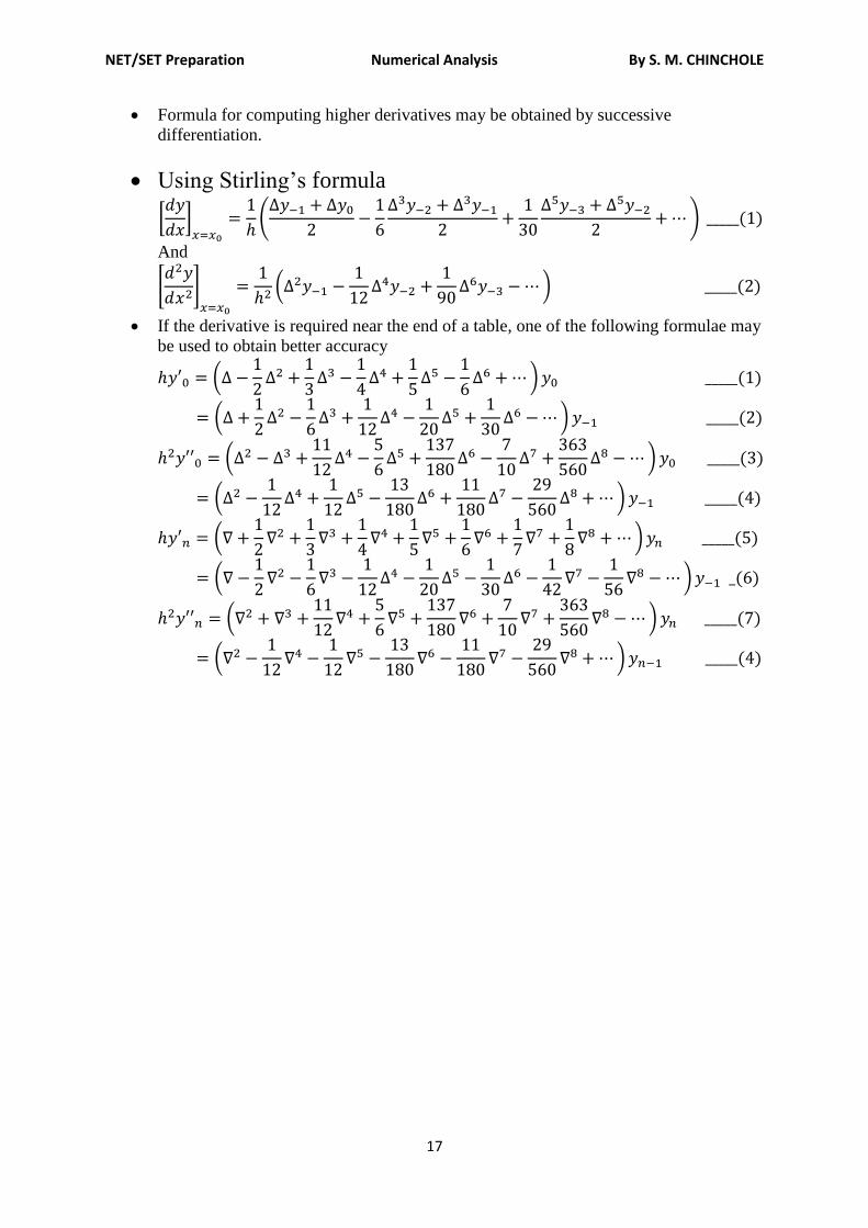
Formula for computing higher derivatives may be obtained by successive

differentiation.

Using Stirling’s formula

[

]

(

)

And

*

+

(

)

If the derivative is required near the end of a table, one of the following formulae may

be used to obtain better accuracy

(

)

(

)

(

)

(

)

(

)

(

)

(

)

(

)


18

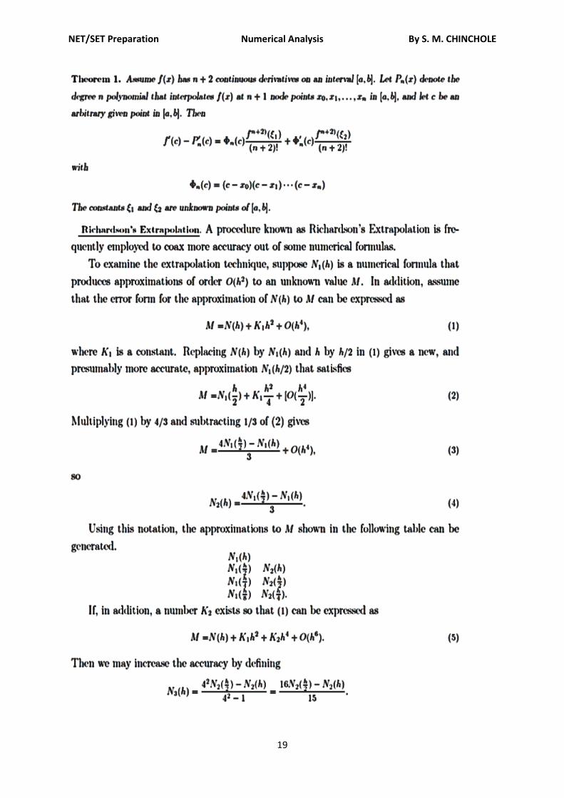
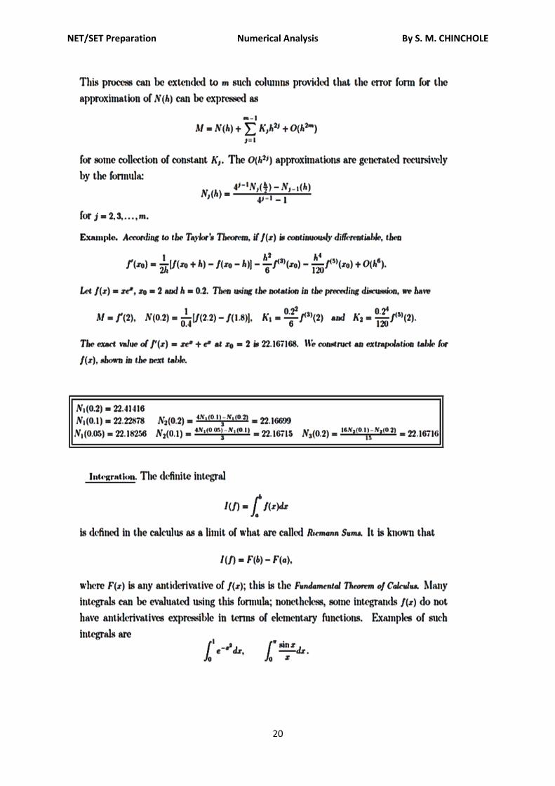
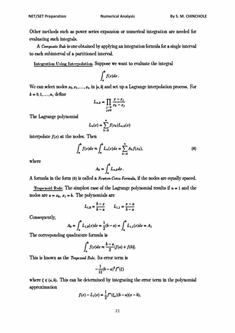
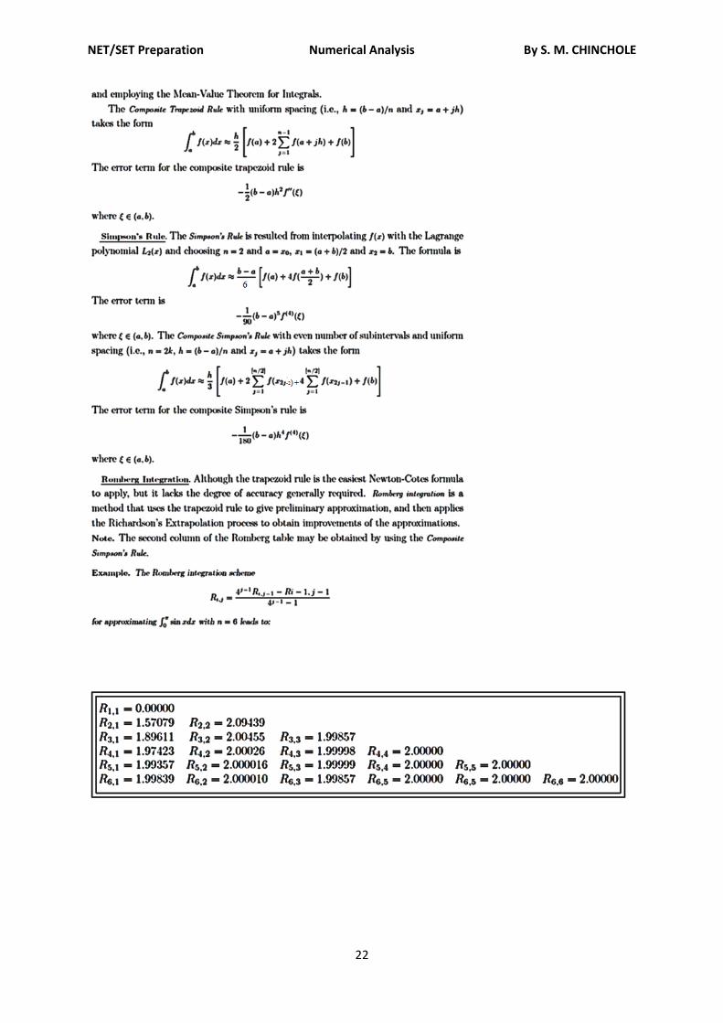
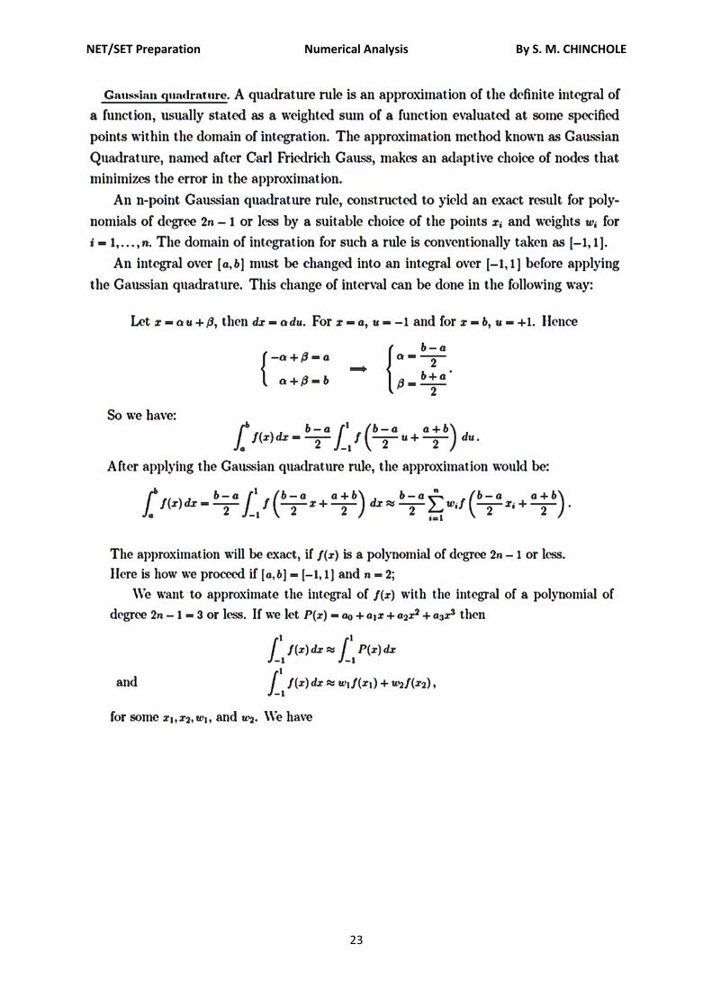
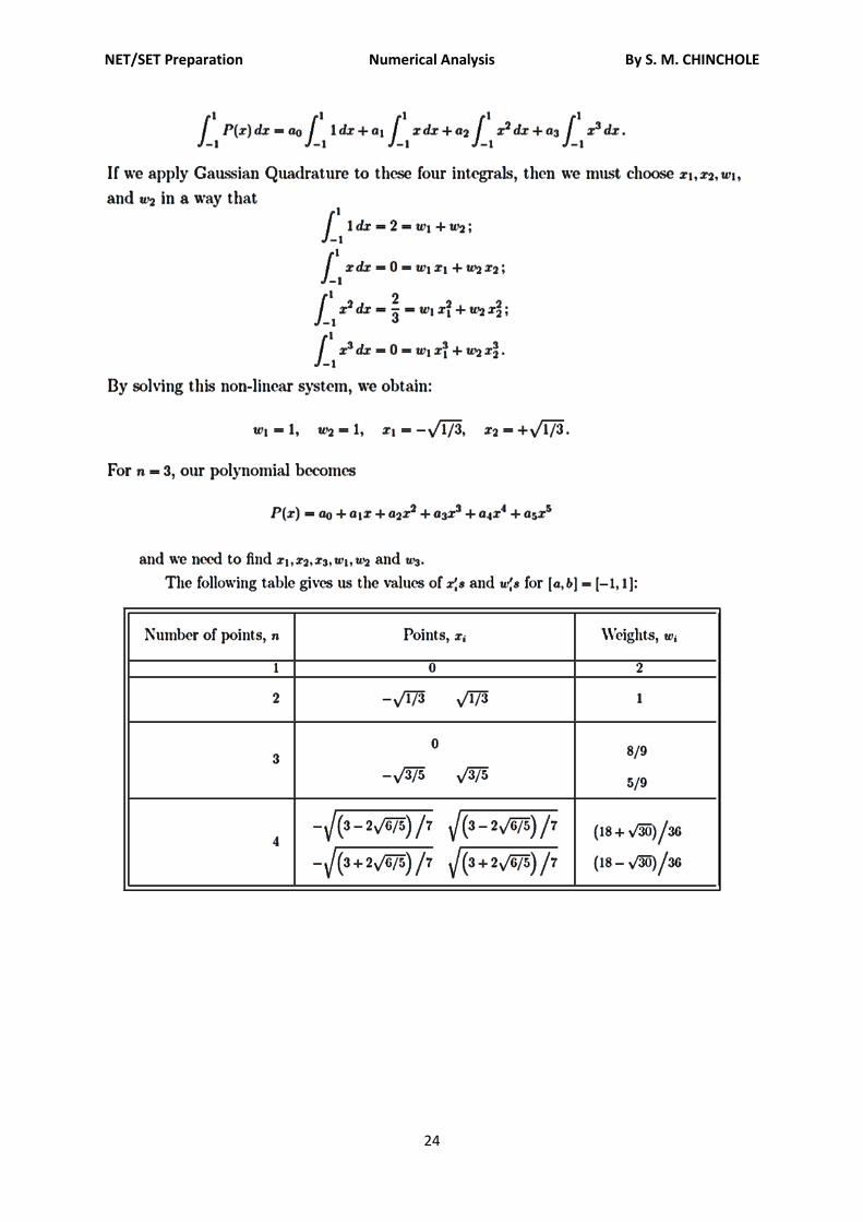
NUMERICAL DIFFERENTIATION AND INTEGRATION


19


20


21


22


23


24


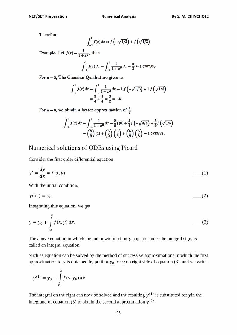
25

Numerical solutions of ODEs using Picard

Consider the first order differential equation

With the initial condition,

Integrating this equation, we get

∫

The above equation in which the unknown function appears under the integral sign, is

called an integral equation.

Such as equation can be solved by the method of successive approximations in which the first

approximation to is obtained by putting for on right side of equation (3), and we write

∫

The integral on the right can now be solved and the resulting is substituted for in the

integrand of equation (3) to obtain the second approximation :


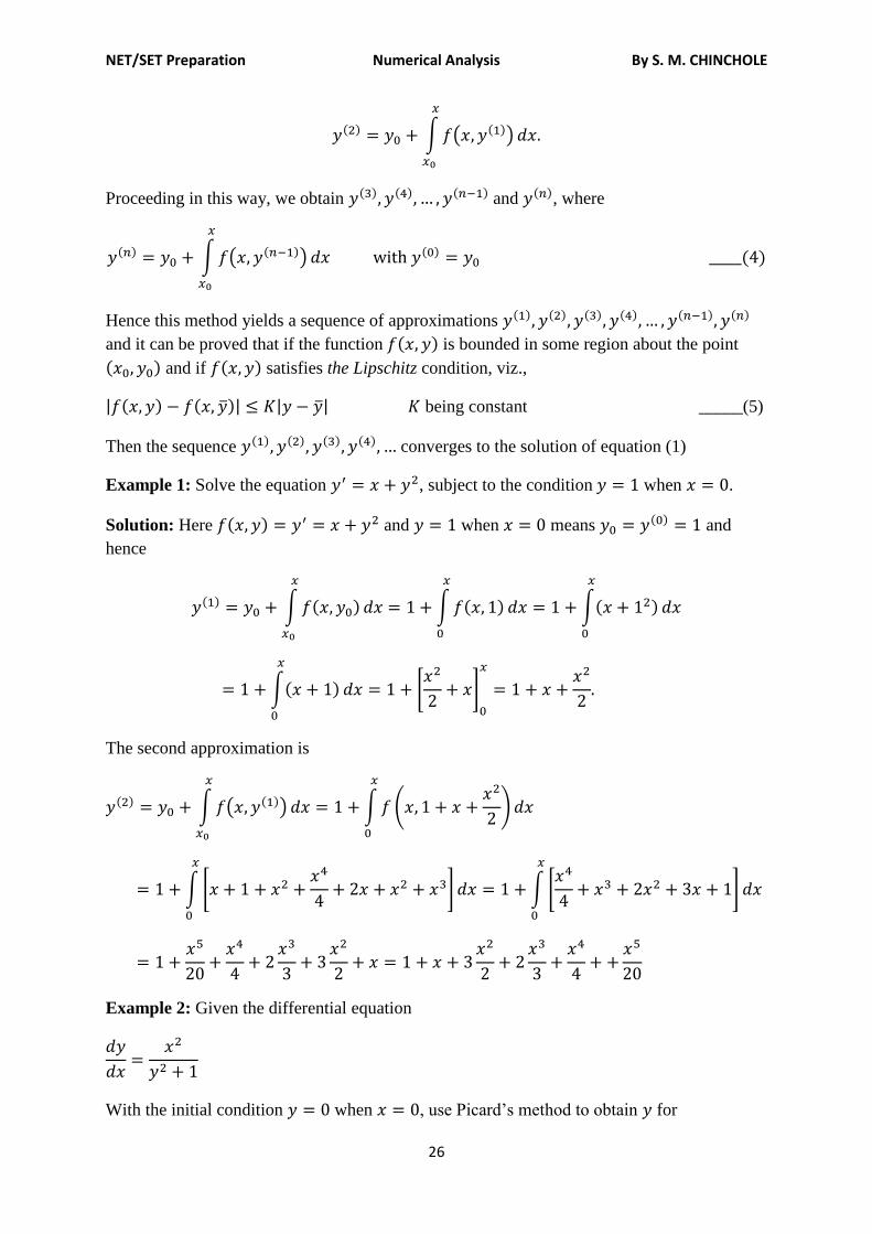
26

∫ ( )

Proceeding in this way, we obtain and , where

∫ ( )

Hence this method yields a sequence of approximations

and it can be proved that if the function is bounded in some region about the point

and if satisfies the Lipschitz condition, viz.,

| ̅ | | ̅| being constant _____(5)

Then the sequence converges to the solution of equation (1)

Example 1: Solve the equation , subject to the condition when .

Solution: Here and when means and

hence

∫

∫

∫

∫

*

+

The second approximation is

∫ ( )

∫ (

)

∫ *

+

∫ *

+

Example 2: Given the differential equation

With the initial condition when , use Picard’s method to obtain for


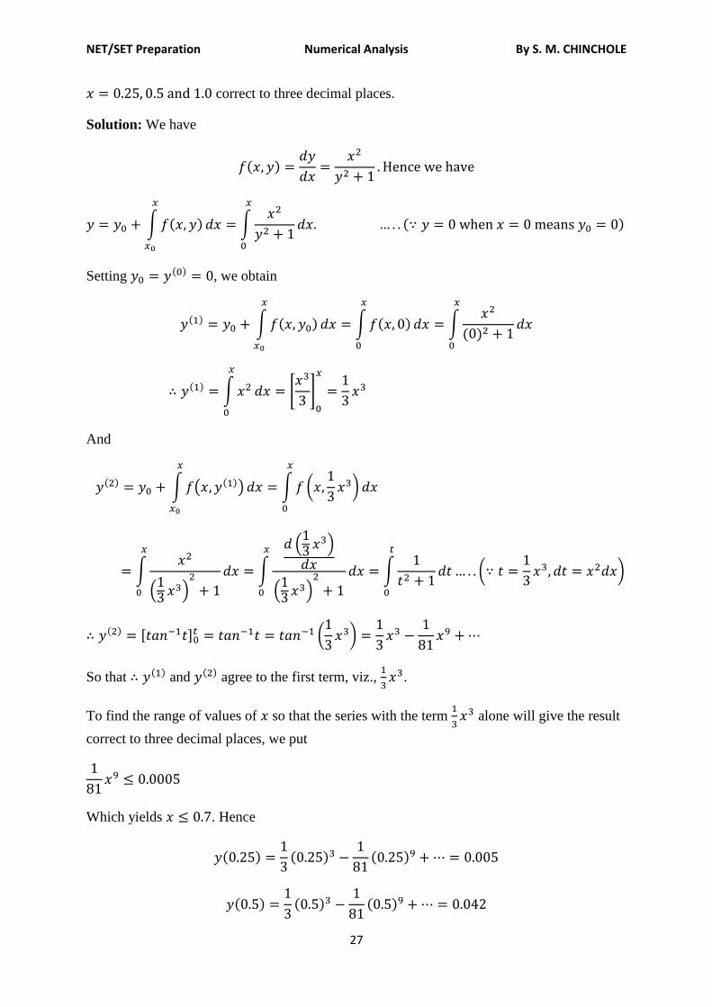
27

correct to three decimal places.

Solution: We have

∫

∫

Setting , we obtain

∫

∫

∫

∫

*

+

And

∫ ( )

∫ (

)

∫

( )

∫

( )

( )

∫

(

)

[ ] (

)

So that and agree to the first term, viz.,

.

To find the range of values of so that the series with the term

alone will give the result

correct to three decimal places, we put

Which yields . Hence


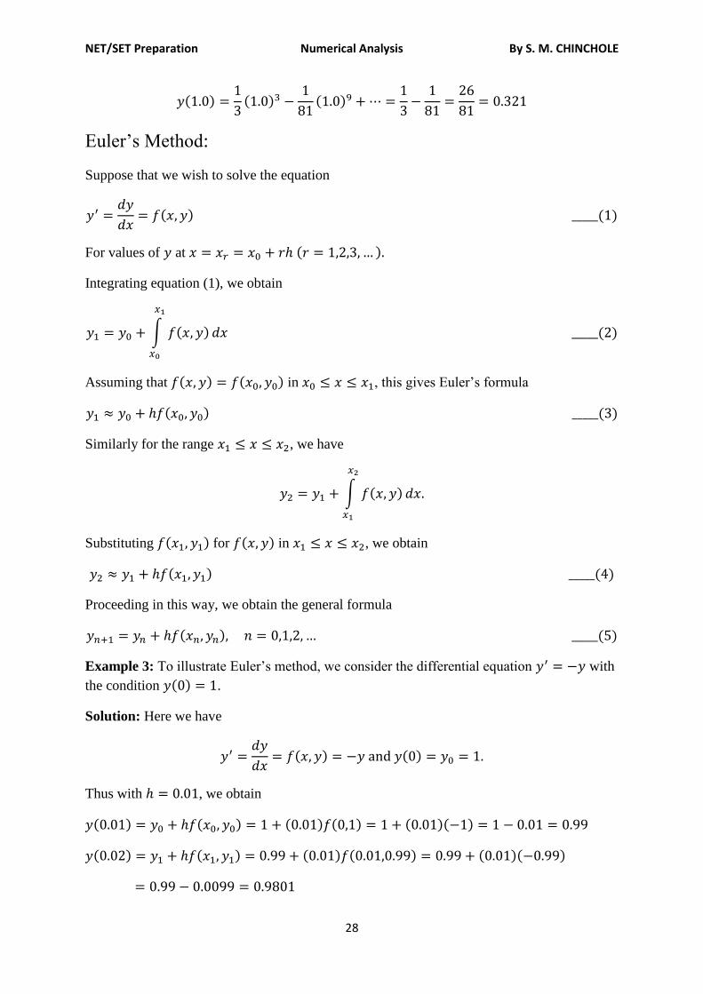
28

Euler’s Method:

Suppose that we wish to solve the equation

For values of at

Integrating equation (1), we obtain

∫

Assuming that in , this gives Euler’s formula

Similarly for the range , we have

∫

Substituting for in , we obtain

Proceeding in this way, we obtain the general formula

Example 3: To illustrate Euler’s method, we consider the differential equation with

the condition .

Solution: Here we have

Thus with , we obtain


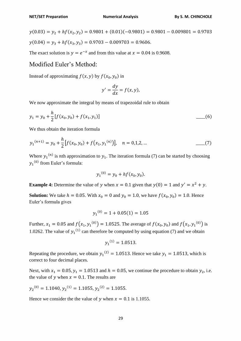
29

.

The exact solution is and from this value at is 0.9608.

Modified Euler’s Method:

Instead of approximating by in

We now approximate the integral by means of trapezoidal rule to obtain

[ ]

We thus obtain the iteration formula

[ (

)]

Where is th approximation to . The iteration formula (7) can be started by choosing

from Euler’s formula:

Example 4: Determine the value of when given that and .

Solution: We take . With and we have Hence

Euler’s formula gives

Further, and ( ) The average of and (

) is

1.0262. The value of can therefore be computed by using equation (7) and we obtain

Repeating the procedure, we obtain Hence we take which is

correct to four decimal places.

Next, with and we continue the procedure to obtain i.e.

the value of when . The results are

Hence we consider the the value of when is 1.1055.


30

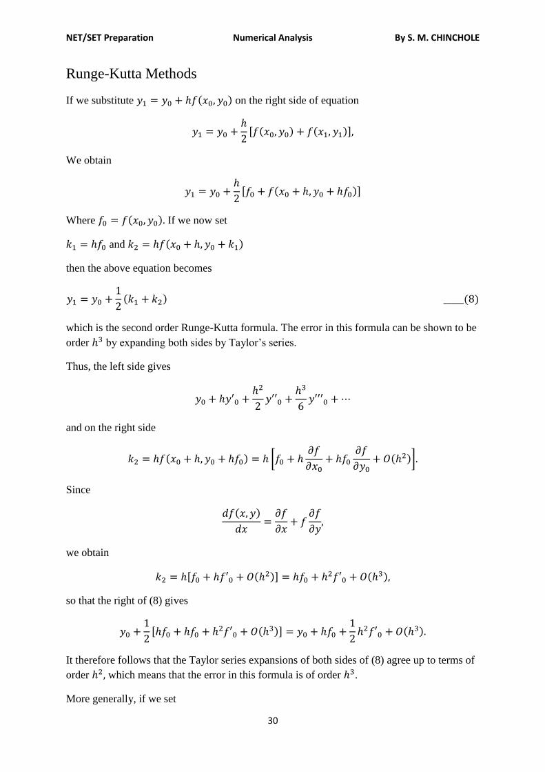
Runge-Kutta Methods

If we substitute on the right side of equation

[ ]

We obtain

[ ]

Where If we now set

and

then the above equation becomes

which is the second order Runge-Kutta formula. The error in this formula can be shown to be

order by expanding both sides by Taylor’s series.

Thus, the left side gives

and on the right side

[

]

Since

we obtain

[ ]

so that the right of (8) gives

[ ]

It therefore follows that the Taylor series expansions of both sides of (8) agree up to terms of

order which means that the error in this formula is of order .

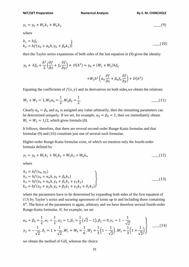
More generally, if we set


31

where

}

then the Taylor series expansions of both sides of the last equation in (9) gives the identity

(

)

(

)

Equating the coefficients of and its derivatives on both sides,we obtain the relations

Clearly and is assigned any value arbitrarily, then the remaining parameters can

be determined uniquely. If we set, for example, then we immediately obtain

which gives formula (8).

It follows, therefore, that there are several second-order Runge-Kutta formulas and that

formulae (9) and (10) constitute just one of several such formulae.

Higher-order Runge-Kutta formulae exist, of which we mention only the fourth-order

formula defined by

where

}

where the parameters have to be determined by expanding both sides of the first equation of

(13) by Taylor’s series and securing agreement of terms up to and including those containing

. The hoice of the parameters is again, arbitrary and we have therefore several fourth-order

Runge-Kutta formulae. If, for example, we set

(√ )

√

√

√

(

√ )

(

√ )}

we obtain the method of Gill, whereas the choice


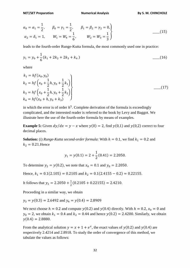
32

}

leads to the fourth-order Runge-Kutta formula, the most commonly used one in practice:

where

(

)

(

)

}

in which the error is of order . Complete derivation of the formula is exceedingly

complicated, and the interested reader is referred to the book by Levy and Baggot. We

illustrate here the use of the fourth-order formula by means of examples.

Example 5: Given ⁄ where , find and correct to four

decimal places.

Solution: (i) Runge-Kutta second-order formula: With , we find and

.Hence

To determine , we note that and .

Hence, and .

It follows that

.

Proceeding in a similar way, we obtain

and

We next choose and compute and directly. With , and

, we obtain and and hence Similarly, we obtain

.

From the analytical solution , the exact values of and are

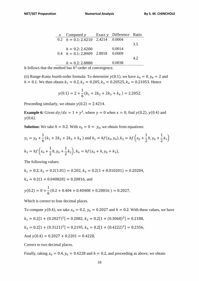
respectively 2.4214 and 2.8918. To study the order of convergence of this method, we

tabulate the values as follows:


33

Computed Exact Difference Ratio

0.2 2.4214 0.0004

3.5

0.0014

0.4 2.8918 0.0009

4.2

0.0038

It follows that the method has -order of convergence.

(ii) Runge-Kutta fourth-order formula: To determine we have and

. We then obtain Hence

Proceeding similarly, we obtain .

Example 6: Given ⁄ where when , find and

.

Solution: We take . With we obtain from equations:

(

)

(

)

The following values:

and

Which is correct to four decimal places.

To compute we take , and With these values, we have

[ ] [ ]

[ ] [ ]

And

Correct to two decimal places.

Finally, taking and and proceeding as above, we obtain


34

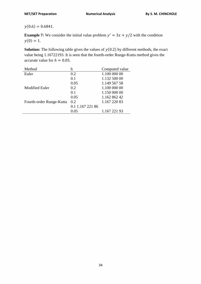
Example 7: We consider the initial value problem with the condition

Solution: The following table gives the values of by different methods, the exact

value being 1.16722193. It is seen that the fourth-order Runge-Kutta method gives the

accurate value for

Method h Computed value

Euler 0.2 1.100 000 00

0.1 1.132 500 00

0.05 1.149 567 58

Modified Euler 0.2 1.100 000 00

0.1 1.150 000 00

0.05 1.162 862 42

Fourth-order Runge-Kutta 0.2 1.167 220 83

0.1 1.167 221 86

0.05 1.167 221 93

NUMERICAL ANALYSIS Numerical solutions of algebraic ...mathskthm.6te.net/Numerical Analysis...

Documents

Transcript of NUMERICAL ANALYSIS Numerical solutions of algebraic ...mathskthm.6te.net/Numerical Analysis...