Num. Meth. Intermezzo on (Numerical) Linear Algebra

2Intermezzo on (Numerical)

Linear Algebra

Let A be an n× n-matrix.

Note that the result of the multiplication of the matrix A with a vector x is a linear combination of the

columns of A:

Ax =n∑

i=1xiA:,i GradinaruD-MATH

p. 1112.0Num.Meth.Phys.

Nonsingu lar Singu larA is invertible A is not invertibleThe columns are independent The columns are dependentThe rows are independent The rows are dependentdet A 6= 0 det A = 0Ax = 0 has one solution x = 0 Ax = 0 has infinitely many solutionsAx = b has one solution x = A−1b Ax = b has no solution or infinetly manyA has full rank A has rank r < nA has n nonzero pivots A has r < n pivotsspan{A:,1, . . . , A:,n} has dimension n span{A:,1, . . . , A:,n} has dimension r < nspan{A1,:, . . . , An,:} has dimension n span{A1,:, . . . , An,:} has dimension r < nAll eigenvalues of A are nonzero 0 is eigenvalue of A0 6∈ σ(A) = Spectrum of A 0 ∈ σ(A)

AHA is symmetric positive definite AHA is only semidefiniteA has n (positive) singular values A has r < n (positive) singular values

Essential Decompositions

(1) Gaussian-elimination is nothing than LU-decomposition: A = LU with lower triangular matrix L

having ones on the main diagonal

Example 2.0.1 (Gaussian elimination and LU-factorization).

GradinaruD-MATHp. 1122.0

Num.Meth.Phys.

consider (forward) Gaussian elimination:

1 1 02 1 −13 −1 −1

x1x2x3

=

41−3

←→

x1 + x2 = 42x1 + x2 − x3 = 13x1 − x2 − x3 = −3

.

11

1

1 1 02 1 −13 −1 −1

41−3

=⇒

12 1

0 1

1 1 00 −1 −13 −1 −1

4−7−3

=⇒

12 13 0 1

1 1 00 −1 −10 −4 −1

4−7−15

=⇒

12 13 4 1

︸︷︷︸=L

1 1 00 −1 −10 0 3

︸︷︷︸=U

4−713

= pivot row, pivot element bold, negative multipliers red3

Perspective: link Gaussian elimination to matrix factorization(row transformation = multiplication with elimination matrix)

a1 6= 0

1 0 · · · · · · 0

−a2

a11 0

−a3

a1

...

−ana1

0 1

a1

a2

a3

...

an

=

a1

0

0...

0

.


Num.Meth.Phys.

n− 1 steps of Gaussian elimination: =⇒ matrix factorization

(non-zero pivot elements assumed)

A = L1 · · · · · Ln−1U withelimination matrices Li, i = 1, . . . , n− 1 ,upper triangular matrix U ∈ R

n,n .

1 0 · · · · · · 0

l2 1 0

l3...

ln 0 1

1 0 · · · · · · 0

0 1 0

0 h3 1... ...

0 hn 0 1

=

1 0 · · · · · · 0

l2 1 0

l3 h3 1... ...

ln hn 0 1

L1 · · · · · Ln−1 are normalized lower triangular matrices

(entries = multipliers −aikakk

)


Num.Meth.Phys.

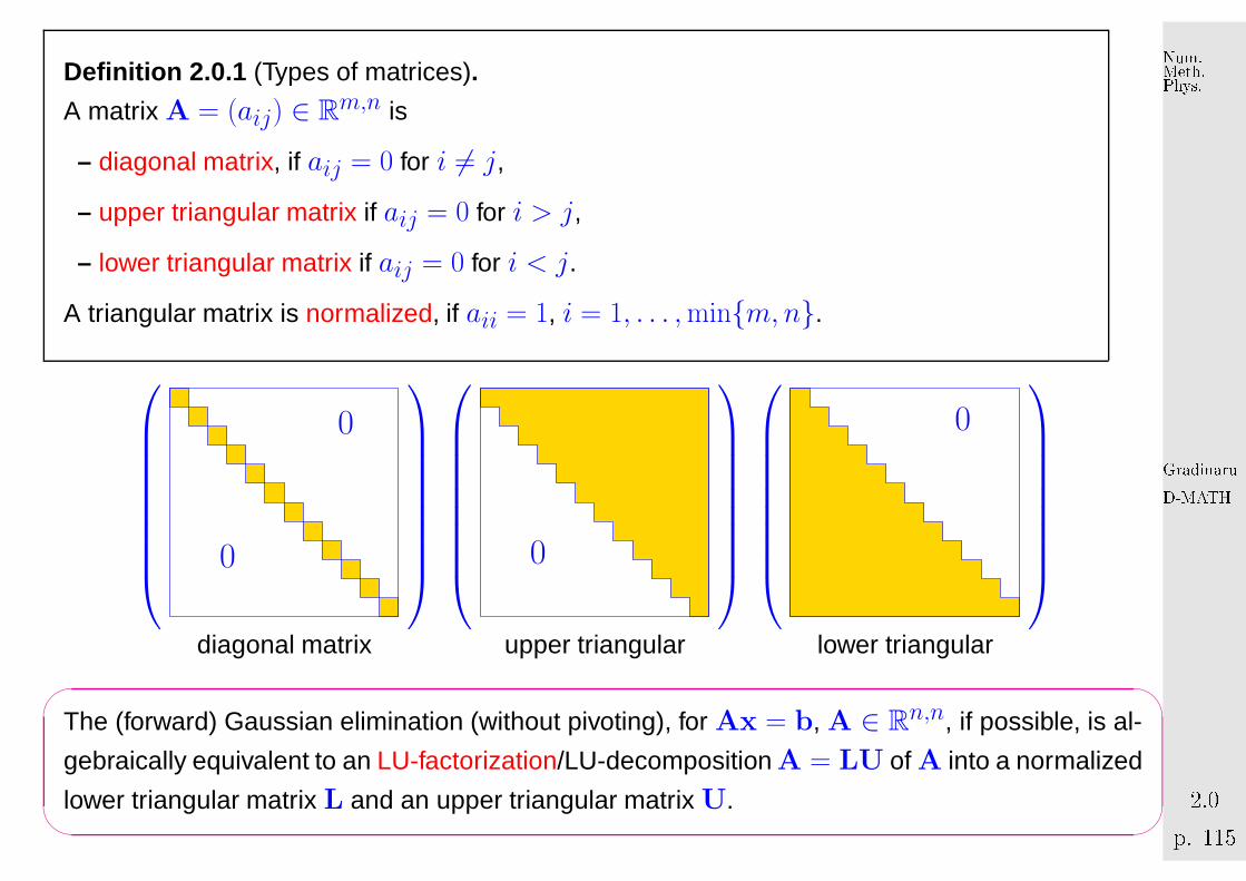
Defin ition 2.0.1 (Types of matrices).

A matrix A = (aij) ∈ Rm,n is

– diagonal matrix, if aij = 0 for i 6= j,

– upper triangular matrix if aij = 0 for i > j,

– lower triangular matrix if aij = 0 for i < j.

A triangular matrix is normalized, if aii = 1, i = 1, . . . , min{m, n}.

0

0

0

0

diagonal matrix upper triangular lower triangular'

&

$

%

The (forward) Gaussian elimination (without pivoting), for Ax = b, A ∈ Rn,n, if possible, is al-

gebraically equivalent to an LU-factorization/LU-decomposition A = LU of A into a normalized

lower triangular matrix L and an upper triangular matrix U.


Num.Meth.Phys.

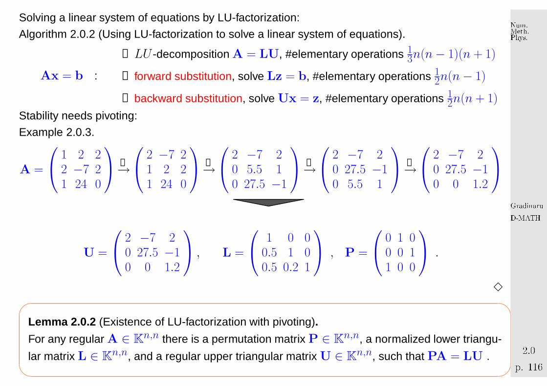
Solving a linear system of equations by LU-factorization:

Algorithm 2.0.2 (Using LU-factorization to solve a linear system of equations).

Ax = b :

① LU -decomposition A = LU, #elementary operations 13n(n− 1)(n + 1)

② forward substitution, solve Lz = b, #elementary operations 12n(n− 1)

③ backward substitution, solve Ux = z, #elementary operations 12n(n + 1)

Stability needs pivoting:

Example 2.0.3.

A =

1 2 22 −7 21 24 0

➊→

2 −7 21 2 21 24 0

➋→

2 −7 20 5.5 10 27.5 −1

➌→

2 −7 20 27.5 −10 5.5 1

➍→

2 −7 20 27.5 −10 0 1.2

U =

2 −7 20 27.5 −10 0 1.2

, L =

1 0 00.5 1 00.5 0.2 1

, P =

0 1 00 0 11 0 0

.

3'

&

$

%

Lemma 2.0.2 (Existence of LU-factorization with pivoting).

For any regular A ∈ Kn,n there is a permutation matrix P ∈ Kn,n, a normalized lower triangu-

lar matrix L ∈ Kn,n, and a regular upper triangular matrix U ∈ K

n,n, such that PA = LU .


Num.Meth.Phys.

python-function: LU, piv = scipy.linalg.lu factor(A)

LU = Matrix containing U in its upper triangle, and L in its lower triangle;

piv = pivot indices representing the permutation matrix P: row i of matrix was interchanged with

row piv[i]

Round-off errors can be dangerous.

Defin ition 2.0.3 (Condition (number) of a matrix).

Condition (number) of a matrix A ∈ Rn,n: cond(A) :=∥∥∥A−1

∥∥∥ ‖A‖

Note:

cond(A) depends on ‖·‖ !

If cond(A)≫ 1, small perturbations in A can lead to large relative errors in the solution of the

LSE.��

��If cond(A)≫ 1, an algorithm can produce solutions with large relative error !

(1’) If A is symmetric, then A = LDLH = RHR with diagonal matrix D containing the pivots

(Choleski-decomposition) and R =√

DLH . No pivoting is necessary.

python-function: scipy.linalg.cho factor(A)


Num.Meth.Phys.

(2) Orthogonalisation: A = QR with the matrix Q having orthonormal columns: QHQ = QQH = I

(see below)

(3) Singular value decomposition (SVD):

A = UΣVH

where each of the matrices U and V have orthonormal columns,

Σ = diag(σ1, . . . , σr, 0, ]ldots, 0), r = rank(A), σ1 ≥ σ2 ≥ σr > 0. Actually, σ21, . . . , σ

2r are the

eigenvalues of AHA (see below).

(4) Schur-decomposition:

∀A ∈ Kn,n: ∃U ∈ C

n,n unitary: UHAU = T with T ∈ Cn,n upper triangular .

Remark 2.0.4. All presented python-functions are in fact wrappers to LAPACK Fortran- or C-routines.

△Remark 2.0.5. Not discussed in this lecture, but of essential importance in applications are the sparse

matrices (i.e. having the number of non-zero elements much smaller than n). Special storing

schemes and algorithms can sometimes keep the factors L and U sparse, but in general this is

difficult or impossible. For such cases, iterative method s for LSE (as e.g. preconditioned conjugate

gradient) are the methods of choice.△


Num.Meth.Phys.

2.1 QR-Factorization/QR-decomposition

Recall from linear algebra:

Defin ition 2.1.1 (Unitary and orthogonal matrices).

•Q ∈ Kn,n, n ∈ N, is unitary, if Q−1 = QH .

•Q ∈ Rn,n, n ∈ N, is orthogonal, if Q−1 = QT .

'

&

$

%

Theorem 2.1.2 (Criteria for Unitarity).

Q ∈ Cn,n unitary ⇔ ‖Qx‖2 = ‖x‖2 ∀x ∈ K

n .

Q unitary ⇒ cond(Q) = 1(?? )➤ unitary transformations enhance (numerical) stability

If Q ∈ Kn,n unitary, then


Num.Meth.Phys.

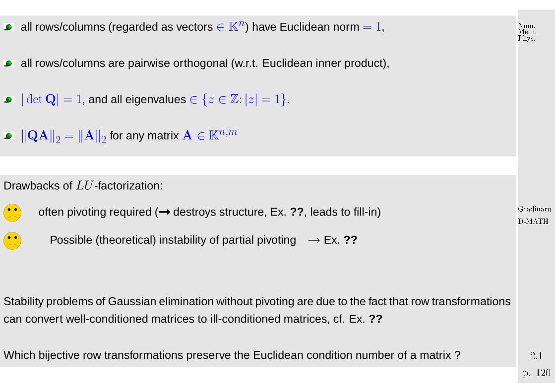
all rows/columns (regarded as vectors ∈ Kn) have Euclidean norm = 1,

all rows/columns are pairwise orthogonal (w.r.t. Euclidean inner product),

| detQ| = 1, and all eigenvalues ∈ {z ∈ Z: |z| = 1}.

‖QA‖2 = ‖A‖2 for any matrix A ∈ Kn,m

Drawbacks of LU -factorization:

often pivoting required (➞ destroys structure, Ex. ?? , leads to fill-in)

Possible (theoretical) instability of partial pivoting → Ex. ??

Stability problems of Gaussian elimination without pivoting are due to the fact that row transformations

can convert well-conditioned matrices to ill-conditioned matrices, cf. Ex. ??

Which bijective row transformations preserve the Euclidean condition number of a matrix ?


Num.Meth.Phys.

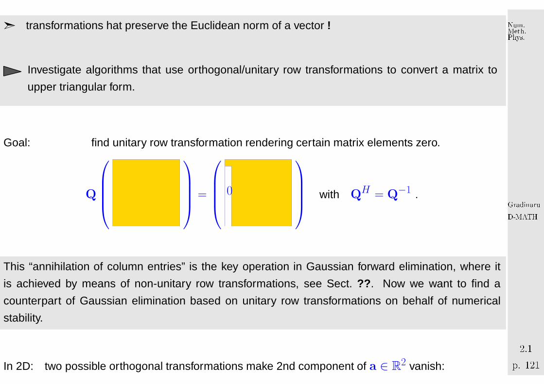
➣ transformations hat preserve the Euclidean norm of a vector !

Investigate algorithms that use orthogonal/unitary row transformations to convert a matrix to

upper triangular form.

Goal: find unitary row transformation rendering certain matrix elements zero.

Q

=

0

with QH = Q−1 .

This “annihilation of column entries” is the key operation in Gaussian forward elimination, where it

is achieved by means of non-unitary row transformations, see Sect. ?? . Now we want to find a

counterpart of Gaussian elimination based on unitary row transformations on behalf of numerical

stability.

In 2D: two possible orthogonal transformations make 2nd component of a ∈ R2 vanish:


Num.Meth.Phys.

. x1

x2

a

Fig. 25

reflection at angle bisector,

. x1

x2

a

ϕ

Q =(

cos ϕ sin ϕ− sinϕ cos ϕ

)

Fig. 26

rotation turning a onto x1-axis.

➣ Note: two possible reflections/rotations

In nD: given a ∈ Rn find orthogonal matrix Q ∈ R

n,n such that Qa = ‖a‖2 e1, e1 = 1st unit

vector.

Choice 1: Householder reflections

Q = H(v) := I− 2vvH

vHvwith v = 1

2(a± ‖a‖2 e1) . (2.1.1)


Num.Meth.Phys.

“Geometric derivation” of Householder reflection, see Figure 25

Given a,b ∈ Rn with ‖a‖ = ‖b‖, the difference

vector v = b− a is orthogonal to the bisector.

a

b

v

Fig. 27

b = a− (a− b) = a− vvTv

vTv= a− 2v

vTa

vTv= a− 2

vvT

vTva = H(v)a ,

because, due to orthogonality (a− b) ⊥ (a + b)

(a− b)T (a− b) = (a− b)T (a− b + a + b) = 2(a− b)Ta .

Remark 2.1.1 (Details of Householder reflections).


Num.Meth.Phys.

• Practice: for the sake of numerical stability (in order to avoid so-called cancellation) choose

v =

{12(a + ‖a‖2 e1) , if a1 > 0 ,12(a− ‖a‖2 e1) , if a1 ≤ 0 .

However, this is not really needed [?, Sect. 19.1] !

• If K = C and a1 = |a1| exp(iϕ), ϕ ∈ [0, 2π[, then choose

v = 12(a± ‖a‖2 e1 exp(−iϕ)) in (2.1.1).

• efficient storage of Householder matrices→ [?]

△


Num.Meth.Phys.

Choice 2: successive Givens rotations (→ 2D case)

G1k(a1, ak)A :=

γ · · · σ · · · 0... . . . ... ...−σ · · · γ · · · 0

... ... . . . ...0 · · · 0 · · · 1

a1...

ak...

an

=

a(1)1...0...

an

, ifγ = a1√

|a1|2+|ak|2,

σ =ak√

|a1|2+|ak|2.

(2.1.2)

Transformation to upper triangular form by successive unitary transformations:

➤

0

*

➤

0

*

➤

0

*

.

= “target column a” (determines unitary transformation),

= modified in course of transformations.

Qn−1Qn−2 · · · · ·Q1A = R ,


Num.Meth.Phys.

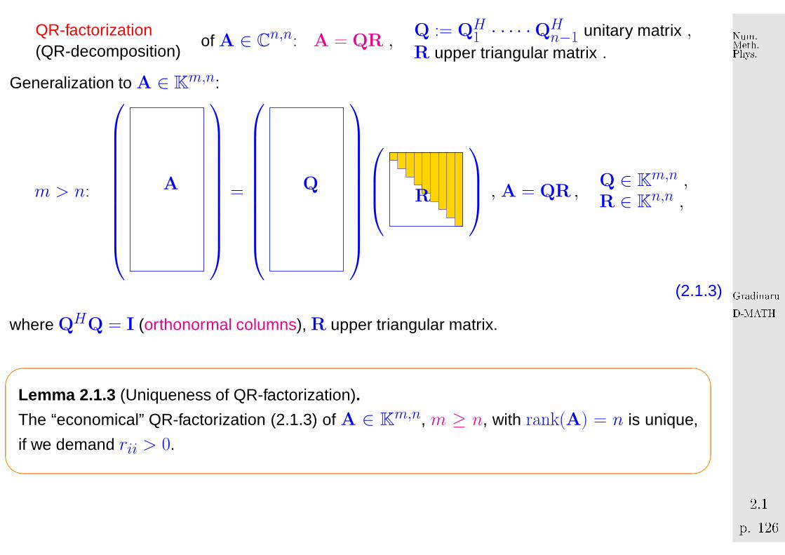
QR-factorization(QR-decomposition)

of A ∈ Cn,n: A = QR ,

Q := QH1 · · · · ·QH

n−1 unitary matrix ,R upper triangular matrix .

Generalization to A ∈ Km,n:

m > n:

A

=

Q

R

, A = QR ,

Q ∈ Km,n ,

R ∈ Kn,n ,

(2.1.3)

where QHQ = I (orthonormal columns), R upper triangular matrix.

'

&

$

%

Lemma 2.1.3 (Uniqueness of QR-factorization).

The “economical” QR-factorization (2.1.3) of A ∈ Km,n, m ≥ n, with rank(A) = n is unique,

if we demand rii > 0.


Num.Meth.Phys.

Proof. we observe that R is regular, if A has full rank n. Since the regular upper triangular matrices

form a group under multiplication:

Q1R1 = Q2R2 ⇒ Q1 = Q2R with upper triangular R := R2R−11 .

I = QH1 Q1 = RH QH

2 Q2︸︷︷︸=I

R = RHR .

The assertion follows by uniqueness of Cholesky decomposition, Lemma ?? . 2

m < n:

A

=

Q

R

,

A = QR , Q ∈ Km,m , R ∈ K

m,n ,

where Q unitary, R upper triangular matrix.

Remark 2.1.2 (Choice of unitary/orthogonal transformation).

When to use which unitary/orthogonal transformation for QR-factorization ?


Num.Meth.Phys.

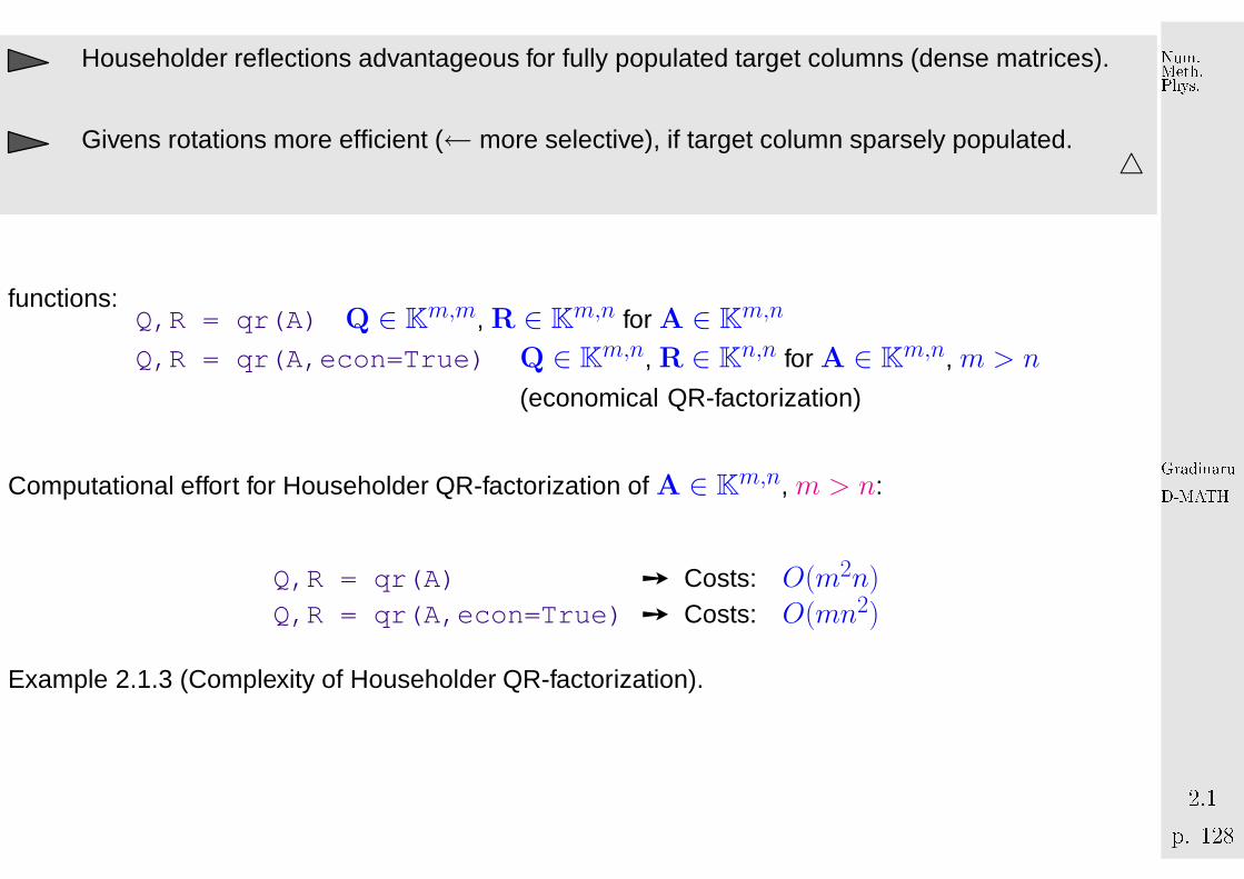
Householder reflections advantageous for fully populated target columns (dense matrices).

Givens rotations more efficient (← more selective), if target column sparsely populated.△

functions:Q,R = qr(A) Q ∈ K

m,m, R ∈ Km,n for A ∈ K

m,n

Q,R = qr(A,econ=True) Q ∈ Km,n, R ∈ Kn,n for A ∈ Km,n, m > n

(economical QR-factorization)

Computational effort for Householder QR-factorization of A ∈ Km,n, m > n:

Q,R = qr(A) ➙ Costs: O(m2n)Q,R = qr(A,econ=True) ➙ Costs: O(mn2)

Example 2.1.3 (Complexity of Householder QR-factorization).


Num.Meth.Phys.

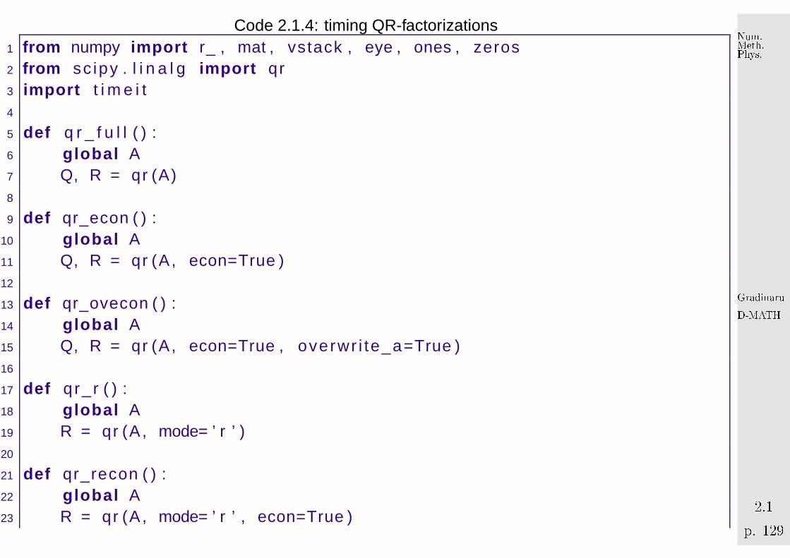
Code 2.1.4: timing QR-factorizations1 from numpy impo r t r_ , mat , vstack , eye , ones , zeros2 from sc ipy . l i n a l g impo r t qr3 impo r t t i m e i t4

5 def q r _ f u l l ( ) :6 g l ob al A7 Q, R = qr (A)8

9 def qr_econ ( ) :10 g l ob al A11 Q, R = qr (A, econ=True )12

13 def qr_ovecon ( ) :14 g l ob al A15 Q, R = qr (A, econ=True , overwr i te_a=True )16

17 def qr_ r ( ) :18 g l ob al A19 R = qr (A , mode= ’ r ’ )20

21 def qr_recon ( ) :22 g l ob al A23 R = qr (A , mode= ’ r ’ , econ=True )


Num.Meth.Phys.

24

25 nrEXP = 426 s izes = 2∗∗ r_ [ 2 : 7 ]27 qr t imes = zeros ( ( 5 , s izes . shape [ 0 ] ) )28 k = 029 f o r n i n s izes :30 p r i n t ’ n= ’ , n31 m = n∗∗2#4*n32 A = mat (1 .∗ r_ [ 1 :m+1 ] ) . T∗mat (1 .∗ r_ [ 1 : n +1 ] )33 A += vstack ( ( eye ( n ) , ones ( (m−n , n ) ) ) )34

35 t = t i m e i t . Timer ( ’ q r _ f u l l ( ) ’ , ’ from __main__ impor t q r _ f u l l ’ )36 avqr = t . t i m e i t ( number=nrEXP ) / nrEXP37 p r i n t avqr38 qr t imes [0 , k ] = avqr39

40 t = t i m e i t . Timer ( ’ qr_econ ( ) ’ , ’ from __main__ impor t qr_econ ’ )41 avqr = t . t i m e i t ( number=nrEXP ) / nrEXP42 p r i n t avqr43 qr t imes [1 , k ] = avqr44

45 t = t i m e i t . Timer ( ’ qr_ovecon ( ) ’ , ’ from __main__ impor t qr_ovecon ’ )46 avqr = t . t i m e i t ( number=nrEXP ) / nrEXP47 p r i n t avqr


Num.Meth.Phys.

48 qr t imes [2 , k ] = avqr49

50 t = t i m e i t . Timer ( ’ q r_ r ( ) ’ , ’ from __main__ impor t q r_ r ’ )51 avqr = t . t i m e i t ( number=nrEXP ) / nrEXP52 p r i n t avqr53 qr t imes [3 , k ] = avqr54

55 t = t i m e i t . Timer ( ’ qr_recon ( ) ’ , ’ from __main__ impor t qr_recon ’ )56 avqr = t . t i m e i t ( number=nrEXP ) / nrEXP57 p r i n t avqr58 qr t imes [4 , k ] = avqr59

60 k += 161

62 #print qrtimes[3]63 impo r t m a t p l o t l i b . pyp lo t as p l t64 p l t . l og log ( s izes , q r t imes [ 0 ] , ’ s ’ , l a b e l= ’ qr ’ )65 p l t . l og log ( s izes , q r t imes [ 1 ] , ’∗ ’ , l a b e l= " qr ( econ=True ) " )66 p l t . l og log ( s izes , q r t imes [ 2 ] , ’ . ’ , l a b e l= " qr ( econ=True ,

overwr i te_a=True ) " )67 p l t . l og log ( s izes , q r t imes [ 3 ] , ’ o ’ , l a b e l= " qr (mode= ’ r ’ ) " )68 p l t . l og log ( s izes , q r t imes [ 4 ] , ’ + ’ , l a b e l= " qr (mode= ’ r ’ , econ=True ) " )69 v4 = qr t imes [1 ,1 ]∗ ( s izes / s izes [ 1 ] ) ∗∗470 v6 = qr t imes [0 ,1 ]∗ ( s izes / s izes [ 1 ] ) ∗∗6


Num.Meth.Phys.

71 p l t . l og log ( s izes , v4 , l a b e l= ’O(n4) ’ )72 p l t . l og log ( s izes , v6 , ’−− ’ , l a b e l= ’O(n6) ’ )73 p l t . legend ( loc =2)74 p l t . x l a b e l ( ’n ’ )75 p l t . y l a b e l ( ’ t ime [ s ] ’ )76 p l t . save f i g ( ’ q r t i m i n g . eps ’ )77 p l t . show ( )

timing of different variants of QR-factorization

100 101 102

n

10-4

10-3

10-2

10-1

100

101

102

tim

e [

s]

qrqr(econ=True)qr(econ=True, overwrite_a=True)

qr(mode='r')qr(mode='r', econ=True)

O(n4 )

O(n6 )

Fig. 283

Remark 2.1.5 (QR-orthogonalization).


Num.Meth.Phys.

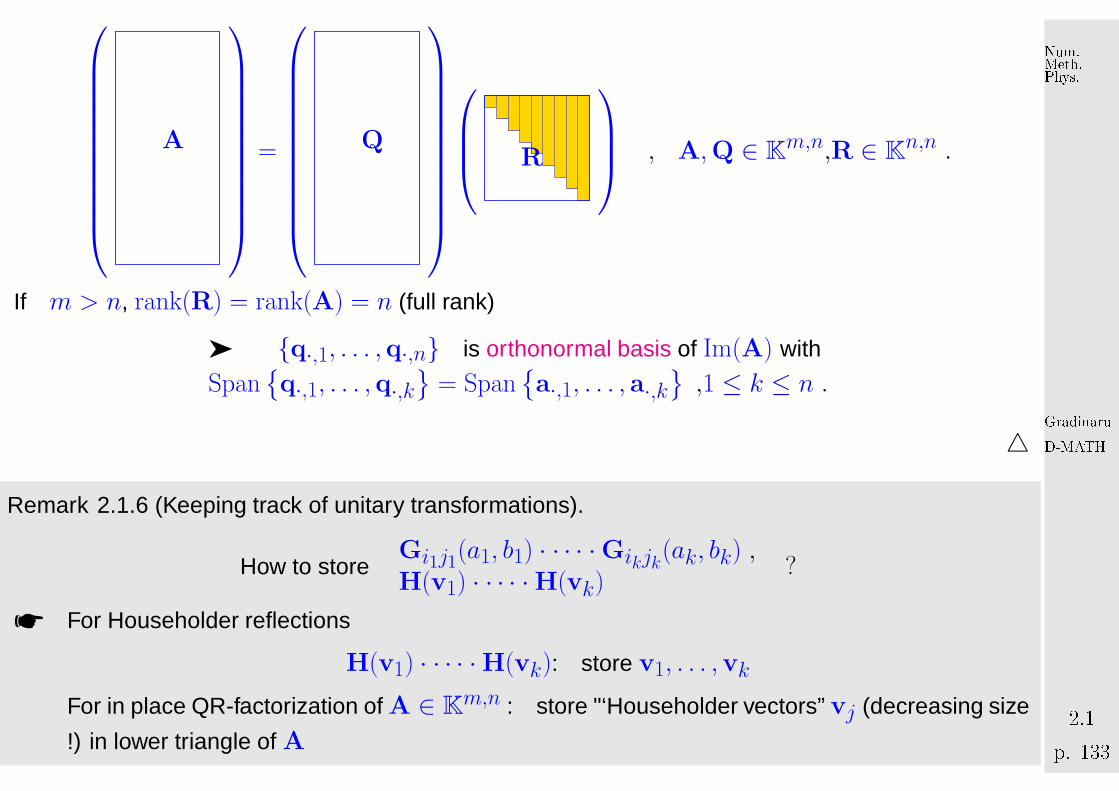
A

=

Q

R

, A,Q ∈ K

m,n,R ∈ Kn,n .

If m > n, rank(R) = rank(A) = n (full rank)

➤ {q·,1, . . . ,q·,n} is orthonormal basis of Im(A) with

Span{q·,1, . . . ,q·,k

}= Span

{a·,1, . . . , a·,k

},1 ≤ k ≤ n .

△

Remark 2.1.6 (Keeping track of unitary transformations).

How to storeGi1j1(a1, b1) · · · · ·Gikjk(ak, bk) ,H(v1) · · · · ·H(vk)

?

☛ For Householder reflections

H(v1) · · · · ·H(vk): store v1, . . . ,vk

For in place QR-factorization of A ∈ Km,n : store "‘Householder vectors” vj (decreasing size

!) in lower triangle of A


Num.Meth.Phys.

R

↑ Case m < n

= Householder vectors

Case m > n→

R

☛ Convention for Givens rotations (K = R)

G =

(γ σ−σ γ

)⇒ store ρ :=

1 , if γ = 0 ,12 sign(γ)σ , if |σ| < |γ| ,2 sign(σ)/γ , if |σ| ≥ |γ| .

ρ = 1 ⇒ γ = 0 , σ = 1

|ρ| < 1 ⇒ σ = 2ρ , γ =√

1− σ2

|ρ| > 1 ⇒ γ = 2/ρ , σ =√

1− γ2 .


Num.Meth.Phys.

Store Gij(a, b) as triple (i, j, ρ)

Storing orthogonal transformation matrices is usually inefficient !

△

Algorithm 2.1.7 (Solving linear system of equations by means of QR-decomposition).

Ax = b :

① QR-decomposition A = QR, computational costs 23n

3 + O(n2) (about twice

as expensive as LU -decomposition without pivoting)

② orthogonal transformation z = QHb, computational costs 4n2 + O(n) (in the

case of compact storage of reflections/rotations)

③ Backward substitution, solve Rx = z, computational costs 12n(n + 1)

'

&

$

%

✌ Computing the generalized QR-decomposition A = QR by means of Householder reflections

or Givens rotations is (numerically stable) for any A ∈ Cm,n.✌ For any regular system matrix an LSE can be solved by means of

QR-decomposition + orthogonal transformation + backward substitution

in a stable manner.


Num.Meth.Phys.

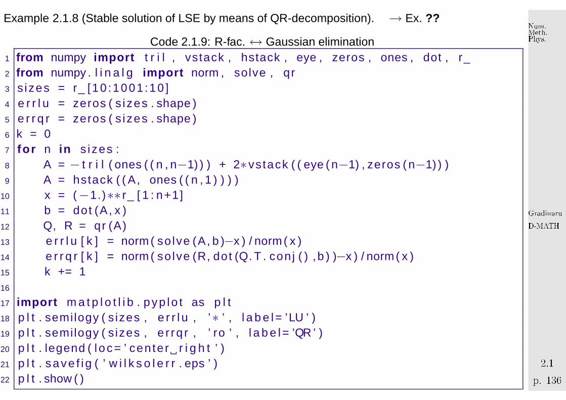
Example 2.1.8 (Stable solution of LSE by means of QR-decomposition). → Ex. ??

Code 2.1.9: R-fac. ↔ Gaussian elimination1 from numpy impo r t t r i l , vstack , hstack , eye , zeros , ones , dot , r_2 from numpy . l i n a l g impo r t norm , solve , qr3 s izes = r_ [10 :1001 :10 ]4 e r r l u = zeros ( s izes . shape )5 e r r q r = zeros ( s izes . shape )6 k = 07 f o r n i n s izes :8 A = − t r i l ( ones ( ( n , n−1) ) ) + 2∗vstack ( ( eye ( n−1) , zeros ( n−1) ) )9 A = hstack ( ( A, ones ( ( n , 1 ) ) ) )

10 x = (−1.)∗∗ r_ [ 1 : n+1]11 b = dot (A, x )12 Q, R = qr (A)13 e r r l u [ k ] = norm ( so lve (A, b )−x ) / norm ( x )14 e r r q r [ k ] = norm ( so lve (R, dot (Q. T . con j ( ) ,b ) )−x ) / norm ( x )15 k += 116

17 impo r t m a t p l o t l i b . pyp lo t as p l t18 p l t . semilogy ( s izes , e r r l u , ’∗ ’ , l a b e l= ’LU ’ )19 p l t . semilogy ( s izes , e r rq r , ’ ro ’ , l a b e l= ’QR ’ )20 p l t . legend ( loc= ’ cen ter r i g h t ’ )21 p l t . save f i g ( ’ w i l k s o l e r r . eps ’ )22 p l t . show ( )


Num.Meth.Phys.

0 100 200 300 400 500 600 700 800 900 1000

10−16

10−14

10−12

10−10

10−8

10−6

10−4

10−2

100

n

rel

ativ

e er

ror

(Euc

lidea

n no

rm)

Gaussian eliminationQR−decompositionrelative residual norm

Fig. 29

� superior stability of QR-decomposition ! 3

Fill-in for QR-decomposition ? bandwidth��

��A ∈ C

n,n with QR-decomposition A = QR ⇒ m(R) ≤ m(A) (→ Def. ?? )


Num.Meth.Phys.

Example 2.1.10 (QR-based solution of tridiagonal LSE).

Elimination of Sub-diagonals by n− 1 successive Givens rotations:

∗ ∗ 0 0 0 0 0 0∗ ∗ ∗ 0 0 0 0 00 ∗ ∗ ∗ 0 0 0 00 0 ∗ ∗ ∗ 0 0 00 0 0 ∗ ∗ ∗ 0 00 0 0 0 ∗ ∗ ∗ 00 0 0 0 0 ∗ ∗ ∗0 0 0 0 0 0 ∗ ∗

G12−−−→

∗ ∗ ∗ 0 0 0 0 00 ∗ ∗ 0 0 0 0 00 ∗ ∗ ∗ 0 0 0 00 0 ∗ ∗ ∗ 0 0 00 0 0 ∗ ∗ ∗ 0 00 0 0 0 ∗ ∗ ∗ 00 0 0 0 0 ∗ ∗ ∗0 0 0 0 0 0 ∗ ∗

G23−−−→ · · ·Gn−1,n−−−−−→

∗ ∗ ∗ 0 0 0 0 00 ∗ ∗ ∗ 0 0 0 00 0 ∗ ∗ ∗ 0 0 00 0 0 ∗ ∗ ∗ 0 00 0 0 0 ∗ ∗ ∗ 00 0 0 0 0 ∗ ∗ ∗0 0 0 0 0 0 ∗ ∗0 0 0 0 0 0 0 ∗

3

2.2 Singu lar Value Decomposition

Remark 2.2.1 (Principal component analysis (PCA)).


Num.Meth.Phys.

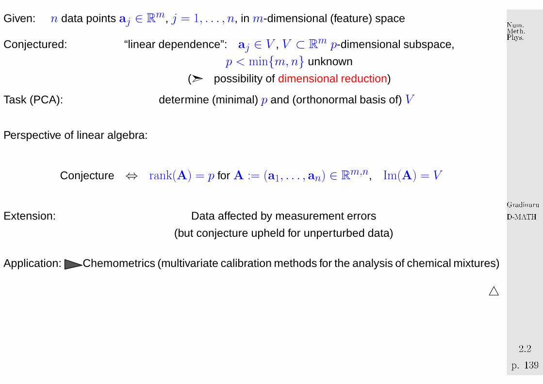
Given: n data points aj ∈ Rm, j = 1, . . . , n, in m-dimensional (feature) space

Conjectured: “linear dependence”: aj ∈ V , V ⊂ Rm p-dimensional subspace,

p < min{m, n} unknown

(➣ possibility of dimensional reduction)

Task (PCA): determine (minimal) p and (orthonormal basis of) V

Perspective of linear algebra:

Conjecture ⇔ rank(A) = p for A := (a1, . . . , an) ∈ Rm,n, Im(A) = V

Extension: Data affected by measurement errors

(but conjecture upheld for unperturbed data)

Application: Chemometrics (multivariate calibration methods for the analysis of chemical mixtures)

△


Num.Meth.Phys.

'

&

$

%

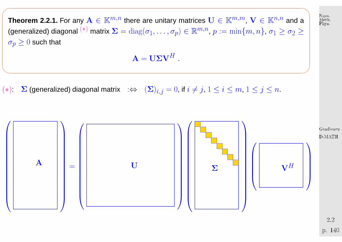
Theorem 2.2.1. For any A ∈ Km,n there are unitary matrices U ∈ K

m,m, V ∈ Kn,n and a

(generalized) diagonal (∗) matrix Σ = diag(σ1, . . . , σp) ∈ Rm,n, p := min{m, n}, σ1 ≥ σ2 ≥σp ≥ 0 such that

A = UΣVH .

(∗): Σ (generalized) diagonal matrix :⇔ (Σ)i,j = 0, if i 6= j, 1 ≤ i ≤ m, 1 ≤ j ≤ n.

A

=

U

Σ

VH


Num.Meth.Phys.

A

=

U

Σ

VH

Proof. (of Thm. 2.2.1, by induction)

[?, Thm. 4.2.3]: Continuous functions attain extremal values on compact sets (here the unit ball{x ∈ Rn: ‖x‖2 ≤ 1})

➤ ∃x ∈ Kn,y ∈ K

m , ‖x‖ = ‖y‖2 = 1 : Ax = σy , σ = ‖A‖2 ,

where we used the definition of the matrix 2-norm, see Def. 1.1.12. ByGram-Schmidt orthogonalization: ∃V ∈ K

n,n−1, U ∈ Km,m−1 such that

V = (x V) ∈ Kn,n , U = (y U) ∈ K

m,m are unitary.

UHAV = (y U)HA(x V) =

(yHAx yHAV

UHAx UHAV

)=

(σ wH

0 B

)=: A1 .


Num.Meth.Phys.

Since∥∥∥∥A1

(σw

)∥∥∥∥2

2=

∥∥∥∥(

σ2 + wHw

Bw

)∥∥∥∥2

2= (σ2 + wHw)2 + ‖Bw‖22 ≥ (σ2 + wHw)2 ,

we conclude

‖A1‖22 = sup0 6=x∈Kn

‖A1x‖22‖x‖22

≥∥∥A1

(σw

)∥∥22∥∥(σ

w

)∥∥22

≥ (σ2 + wHw)2

σ2 + wHw= σ2 + wHw . (2.2.1)

σ2 = ‖A‖22 =∥∥∥UHAV

∥∥∥2

2= ‖A1‖22

(2.2.1)=⇒ ‖A1‖22 = ‖A1‖22 + ‖w‖22 ⇒ w = 0 .

A1 =

(σ 00 B

).

Then apply induction argument to B 2.

Defin ition 2.2.2 (Singular value decomposition (SVD)).

The decomposition A = UΣVH of Thm. 2.2.1 is called singular value decomposition (SVD) of

A. The diagonal entries σi of Σ are the singular values of A.


Num.Meth.Phys.

'

&

$

%

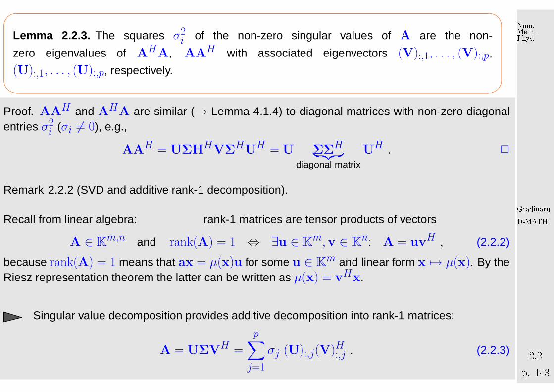
Lemma 2.2.3. The squares σ2i of the non-zero singular values of A are the non-

zero eigenvalues of AHA, AAH with associated eigenvectors (V):,1, . . . , (V):,p,

(U):,1, . . . , (U):,p, respectively.

Proof. AAH and AHA are similar (→ Lemma 4.1.4) to diagonal matrices with non-zero diagonalentries σ2

i (σi 6= 0), e.g.,

AAH = UΣHHVΣHUH = U ΣΣH︸︷︷︸diagonal matrix

UH . 2

Remark 2.2.2 (SVD and additive rank-1 decomposition).

Recall from linear algebra: rank-1 matrices are tensor products of vectors

A ∈ Km,n and rank(A) = 1 ⇔ ∃u ∈ K

m,v ∈ Kn: A = uvH , (2.2.2)

because rank(A) = 1 means that ax = µ(x)u for some u ∈ Km and linear form x 7→ µ(x). By the

Riesz representation theorem the latter can be written as µ(x) = vHx.

Singular value decomposition provides additive decomposition into rank-1 matrices:

A = UΣVH =

p∑

j=1

σj (U):,j(V)H:,j . (2.2.3)


Num.Meth.Phys.

△

Remark 2.2.3 (Uniqueness of SVD).

SVD of Def. 2.2.2 is not (necessarily) unique, but the singular values are.

Assume that A has two singular value decompositions

A = U1Σ1VH1 = U2Σ2V

H2 ⇒ U1 Σ1Σ

H1︸︷︷︸

=diag(s11,...,s1

m)

UH1 = AAH = U2 Σ2Σ

H2︸︷︷︸

=diag(s21,...,s2

m)

UH2 .

Two similar diagonal matrices are equal ! 2

△

Python-function: scipy.linalg.svd

scipy.sparse.linalg.svds in scipy 0.10

SVD on a large sparse matrix: package divisi

python-functions (for algorithms see [?, Sect. 8.3]):


Num.Meth.Phys.

s = svd(A) : computes singular values of matrix A

[U,S,V] = svd(A) : computes singular value decomposition according to Thm. 2.2.1[U,S,V] = svd(A,0) : “economical” singular value decomposition for m > n: : U ∈

Km,n, Σ ∈ Rn,n, V ∈ Kn,n

s = svds(A,k) : k largest singular values (important for sparse A→ Def. ?? )

[U,S,V] = svds(A,k): partial singular value decomposition: U ∈ Km,k, V ∈ K

n,k,

Σ ∈ Rk,k diagonal with k largest singular values of A.

Explanation: “economical” singular value decomposition:

A

=

U

Σ

VH


Num.Meth.Phys.

(python) algorithm for computing SVD is (numerically) stable

Complexity:2mn2 + 2n3 + O(n2) + O(mn) for s = svd(A),

4m2n + 22n3 + O(mn) + O(n2) for [U,S,V] = svd(A),

O(mn2) + O(n3) for [U,S,V]=svd(A,0), m≫ n.

• Application of SVD: computation of rank , kernel and range of a matrix

'

&

$

%

Lemma 2.2.4 (SVD and rank of a matrix).

If the singular values of A satisfy σ1 ≥ · · · ≥ σr > σr+1 = · · · σp = 0, then

• rank(A) = r ,• Ker(A) = Span

{(V):,r+1, . . . , (V):,n

},

• Im(A) = Span{(U):,1, . . . , (U):,r

}.


Num.Meth.Phys.

Illustration: columns = ONB of Im(A) rows = ONB of Ker(A)

A

=

U

0

0 0

Σr

VH

(2.2.4)

Remark: python function r=rank(A) relies on svd(A)

Lemma 2.2.4 PCA by SVD

➊ no perturbations:

SVD: A = UΣVH satisfies σ1 ≥ σ2 ≥ . . . σp > σp+1 = · · · = σmin{m,n} = 0 ,

V = Span {(U):,1, . . . , (U):,p}︸︷︷︸ONB of V

.


Num.Meth.Phys.

➋ with perturbations:

SVD: A = UΣVH satisfies σ1 ≥ σ2 ≥ . . . σp≫σp+1 ≈ · · · ≈ σmin{m,n}≈ 0 ,

V = Span {(U):,1, . . . , (U):,p}︸︷︷︸ONB of V

.

If there is a pronounced gap in distribution of the singular values, which separates p large from

min{m, n} − p relatively small singular values, this hints that Im(A) has essentially dimension p. It

depends on the application what one accepts as a “pronounced gap”.

Example 2.2.4 (Principal component analysis for data analysis).

A ∈ Rm,n, m≫ n:

Columns A → series of measurements at different times/locations etc.Rows of A → measured values corresponding to one time/location etc.

Goal: detect linear correlations

Concrete: two quantities measured over one year at 10 different sites


Num.Meth.Phys.

(Of course, measurements affected by errors/fluc-

tuations)

n = 10; m = 50r = linspace(1,m,m)x = sin(pi*r/m)y = cos(pi*r/m)A = zeros((2*n,m))for k in xrange(n):

A[2*k] = x*rand(m)A[2*k+1] = y+0.1*rand(m)

0 5 10 15 20 25 30 35 40 45 50−1

−0.5

0

0.5

1

1.5

measurement 1measurement 2measurement 2measurement 4 GradinaruD-MATH

p. 1492.2Num.Meth.Phys.

0 2 4 6 8 10 12 14 16 18 200

2

4

6

8

10

12

14

16

No. of singular value

sin

gula

r va

lue

← distribution of singular values of matrix

two dominant singular values !

measurements display linear correlation with two

principal components

principal components = u·,1, u·,2 (leftmost columns of U-matrix of SVD)their relative weights = v·,1, v·,2 (leftmost columns of V-matrix of SVD)


Num.Meth.Phys.

0 5 10 15 20 25 30 35 40 45 50−0.2

−0.15

−0.1

−0.05

0

0.05

0.1

0.15

0.2

0.25

No. of measurement

prin

cipa

l com

pone

nt

1st model vector2nd model vector1st principal component2nd principal component

Fig. 30 0 2 4 6 8 10 12 14 16 18 200

0.05

0.1

0.15

0.2

0.25

0.3

0.35

0.4

measurement

con

trib

utio

n of

prin

cipa

l com

pone

nt

1st principal component2nd principal component

Fig. 313

• Application of SVD: extrema of quadratic forms on the unit sphere

A minimization problem on the Euclidean unit sphere {x ∈ Kn: ‖x‖2 = 1}:

given A ∈ Km,n , m > n, find x ∈ K

n, ‖x‖2 = 1 , ‖Ax‖2 → min . (2.2.5)

Use that multiplication with unitary matrices preserves the 2-norm and the singular value decompo-sition A = UΣVH (→ Def. 2.2.2):

min‖x‖

2=1‖Ax‖22 = min

‖x‖2=1

∥∥∥UΣVHx

∥∥∥2

2= min‖VHx‖

2=1

∥∥∥UΣ(VHx)∥∥∥

2

2


Num.Meth.Phys.

= min‖y‖

2=1‖Σy‖22 = min

‖y‖2=1

(σ21y

21 + · · · + σ2

ny2n) ≥ σ2

n .

The minimum σ2n is attained for y = en ⇒ minimizer x = Ven = (V):,n.

By similar arguments:

σ1 = max‖x‖

2=1‖Ax‖2 , (V):,1 = argmax

‖x‖2=1‖Ax‖2 . (2.2.6)

Recall: 2-norm of the matrix A is defined as the maximum in (2.2.6). Thus we have proved the

following theorem:

'

&

$

%

Lemma 2.2.5 (SVD and Euclidean matrix norm).

• ∀A ∈ Km,n: ‖A‖2 = σ1(A) ,

• ∀A ∈ Kn,n regular: cond2(A) = σ1/σn .

Remark: functions norm(A) and cond(A) rely on svd(A)

Remark: Enchanced PCA in matplotlib.mlab.PCA and in the package MDA (Modular Toolkit

for Data Processing)


Num.Meth.Phys.

2.3 Essential Skill s Learned in Chapter 2

You should know:

• what is the QR-decomposition and possibilities to get it

• what is the singular value decomposition and how to use it

• applications of the svd: principal component analysis, extrema of quadratic forms on the unit

sphere GradinaruD-MATHp. 1532.3

Num.Meth.Phys.

Num. Meth. Intermezzo on (Numerical) Linear Algebra

Documents

Transcript of Num. Meth. Intermezzo on (Numerical) Linear Algebra