NUCLEAR MAGNETIC RESONANCE STUDIES

OF WORMLIKE MICELLES IN

POROUS MEDIA

by

Jacob Donald Trudnowski

A thesis submitted in partial fulfillment

of the requirements for the degree

of

Master of Science

in

Chemical Engineering

MONTANA STATE UNIVERISTY

Bozeman, Montana

January 2016

@COPYRIGHT

by

Jacob Donald Trudnowski

2016

All Rights Reserved

ii

TABLE OF CONTENTS

1. INTRODUCTION ...........................................................................................................1

Complex Fluids: Viscoelastic Wormlike Micelles ..........................................................4

Porous Media ...................................................................................................................7

2. INTRODUCTION TO NUCLEAR MAGNETIC RESONANCE (NMR) .................. 10

Quantum Mechanics of Hydrogen .................................................................................10

Radio Frequency Excitation ...........................................................................................14

Relaxation ......................................................................................................................16

Bloch Equations .............................................................................................................18

Signal Detection .............................................................................................................18

3. ADVANCED NMR TOPICS: GRADIENTS, SEQUENCES, IMAGING,

AND MOTION TRACKING ........................................................................................21

Slice Selection ................................................................................................................22

k-space ...........................................................................................................................23

Motion Tracking: q-space, Diffusion, and Propagators .................................................27

Velocity Imaging ...........................................................................................................31

4. EXPERIMENTAL SETUP AND METHODS ..............................................................33

5. RESULTS AND DISCUSSION ....................................................................................36

Rheology Measurements ................................................................................................36

2D Velocity Images .......................................................................................................38

Propagator Measurements ..............................................................................................39

Dispersion Measurements ..............................................................................................45

Conclusion .....................................................................................................................47

REFERENCES CITED ......................................................................................................48

iii

LIST OF TABLES

Table Page

5.1 Skews of propagators……………………………………………………….44

iv

LIST OF FIGURES

Figure Page

2.1 Precession of magnetic moment…………………………………………….11

2.2 Alignment of magnetic moments…………………………………………....11

2.3 Rotating Frame………………………………………………………………13

2.4 Tipping of magnetization……………………………………………………16

3.1 k-space………………………………………………………………….…...24

3.2 1D imaging sequence………………………………………………….…….25

3.3 PGStE sequence………………………………………………………….….28

3.4 Velocity imaging sequence………………………………………………….32

4.1 Experimental Setup………………………………………………………….34

5.1 Rheology measurements…………………………………………………….36

5.2 2D velocity images………………………………………………………….39

5.3 Water propagators…………………………………………………………...41

5.4 CTAT propagators…………………………………………………………...42

5.5 Comparison of propagators………………………………………………….43

5.6 Dispersion fitting……………………………………………………………46

v

ABSTRACT

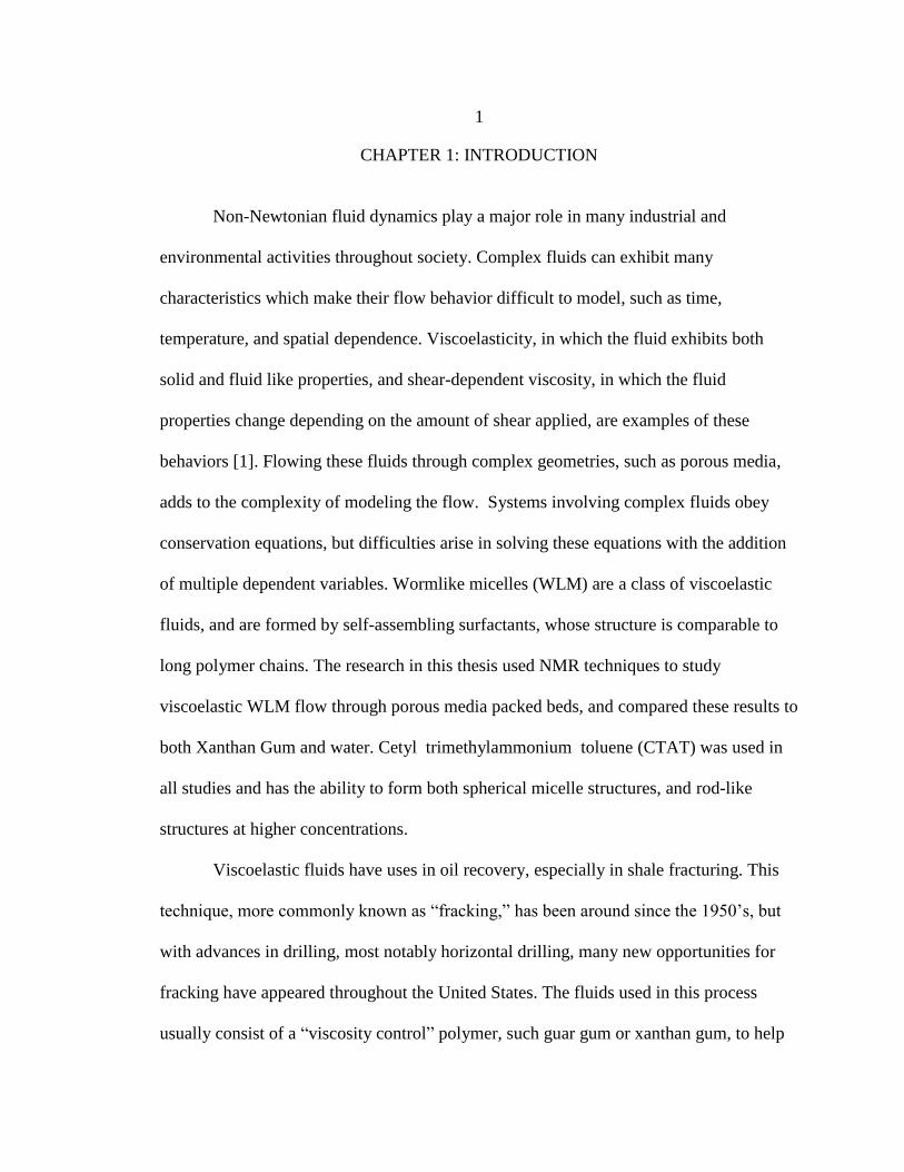
Interest of worm-like micelles (WLM) in porous media has grown in oil industries

as a rock fracturing fluid due to its fluid rheology properties. Non-invasive techniques

like NMR are ideal for observing and monitoring non-Newtonian fluids. This research

presents data collected using NMR techniques with Cetyl trimethyl ammonium toluene

(CTAT) wormlike micelles flowing through porous media. Deviations from Gaussian

behavior in displacement distributions are quantified, and effects of WLM in fluid

flowing through porous media was observed.

1

CHAPTER 1: INTRODUCTION

Non-Newtonian fluid dynamics play a major role in many industrial and

environmental activities throughout society. Complex fluids can exhibit many

characteristics which make their flow behavior difficult to model, such as time,

temperature, and spatial dependence. Viscoelasticity, in which the fluid exhibits both

solid and fluid like properties, and shear-dependent viscosity, in which the fluid

properties change depending on the amount of shear applied, are examples of these

behaviors [1]. Flowing these fluids through complex geometries, such as porous media,

adds to the complexity of modeling the flow. Systems involving complex fluids obey

conservation equations, but difficulties arise in solving these equations with the addition

of multiple dependent variables. Wormlike micelles (WLM) are a class of viscoelastic

fluids, and are formed by self-assembling surfactants, whose structure is comparable to

long polymer chains. The research in this thesis used NMR techniques to study

viscoelastic WLM flow through porous media packed beds, and compared these results to

both Xanthan Gum and water. Cetyl trimethylammonium toluene (CTAT) was used in

all studies and has the ability to form both spherical micelle structures, and rod-like

structures at higher concentrations.

Viscoelastic fluids have uses in oil recovery, especially in shale fracturing. This

technique, more commonly known as “fracking,” has been around since the 1950’s, but

with advances in drilling, most notably horizontal drilling, many new opportunities for

fracking have appeared throughout the United States. The fluids used in this process

usually consist of a “viscosity control” polymer, such guar gum or xanthan gum, to help

2

with the mechanical fracturing process under high pressures. This fluid is typically

recovered with the oil and either recycled on site for further use, or deposited in deep

waste wells. Because of its important applicability to this ever increasing process,

optimization of the fracking fluid properties has gained more interest throughout industry.

Understanding of the fluid is also desired from an environmental standpoint, due to the

fact that not all of the fracking fluid can be recovered [2].

Viscoelastic wormlike micelle solutions have shown a growing use in industrial

processes. Hydraulic fracturing has taken advantage of the enhanced viscosity properties

of WLM solutions for rock fracturing and propping in underground natural gas and oil

recovery. WLM solutions also provide better permeability after fracturing sand pack

pores, allowing for easier separation of fracking fluid and water. This allows for greater

recovery while also reducing formation damage. WLM fracturing also requires fewer

chemical additives when compared to polymer guar gum, and requires no chemical

breakers. [1]

To optimize their use in these applications, it is important to understand the

impact of viscoelasticity on the transport of these fluids in the subsurface. However, the

subsurface is massive in scale and very heterogeneous in structure. Although model

media is usually more homogenous in space than soil, it can provide information about

the fluid moving through tortuous paths in a porous structure. Laboratory experiments

using model porous media can shed light on the fundamental transport dynamics, a

necessary foundation for input into larger and more heterogeneous systems. A true

porous media by definition is a solid with many pores that provide passageway for fluids

to pass through the material. A common example of this would be a household sponge.

3

Sandstone and shale are also considered porous media, which is the most common media

where fracking occurs.

Studies in porous media using model bead packs typically measure pressure

drops. Model porous media are used to study systems relevant to industrial applications;

including catalysis, chromatography, and oil recovery in porous rock [3]. Difficulties in

modeling flow arise due to the separation of length scales [4]. A classic approach in

porous media is to model pores within the bead pack as small capillaries, with dispersion

causing fluid to flow from capillary to capillary. These capillaries and dispersion act on

micron length scales, depending on the pore size, but overall transport through the entire

bead pack can be modeled using macroscopic Darcy’s Law.

Nuclear magnetic resonance (NMR) is an effective, non-invasive, and probe free

method which can gather vital data on transport dynamics in opaque porous media. In

this study, NMR utilizes the interaction of hydrogen molecules’ magnetic moment with a

large magnetic field. NMR can provide 2D and 3D images, velocity images, and

measurement of the probability distribution molecular displacement throughout the

sample, requiring no assumptions about the packing network. This makes NMR a

valuable tool for measuring non-Newtonian fluid flow through porous media, because it

gives displacement information on the pore scale, rather than an average pressure drop

over the entirety of the porous media [5].

4

Complex Fluids: Viscoelastic Wormlike Micelles

Wormlike micelles have shown promising uses in many fields including; natural

gas and oil propagation, as drag reducing agents in heating and cooling systems, and in

home care cleaning products [6]. The ability of WLM’s in solution to form, break apart

and reform cylindrical and spherical microstructures within a fluid can have

advantageous effects in many of these industrial situations.

A fluid’s dynamics can be influenced by the intermolecular and/or intramolecular

forces between molecules. For a Newtonian fluid, such as water, very little of its

rheology is determined by intramolecular or intermolecular forces, and a linear

relationship between shear stress and shear strain with the slope being defined as the

viscosity. For non-Newtonian fluids, more specifically viscoelastic wormlike micelles,

both of these forces show great importance in defining the fluid’s rheology. In non-

Newtonian fluid, the relationship between shear stress and shear strain in not linear, and

has a non-constant viscosity

Intermolecular forces within WLM can create a number of effects which impact

the flow field. Due to the WLM’s long chain, elastic properties, most commonly

associated with polymers, can have great effect on the flow. Both tangential forces and

normal forces become important due the phenomena of micelles relieving stress with

stress in a number of different ways.

WLM are commonly referred to as “living polymers,” for a number of reasons.

Like a polymer, a micelle can relieve physical stress that has been applied to it by

reptation, caused by the random motion of molecules in fluid called Brownian motion.

5

Both fluids can also form entangled networks with each other at higher concentrations.

Unlike a polymer, the micelle does not have a covalently bonded backbone that holds the

structure together, but rather relies on intermolecular forces to hold the “polymer-like”

structure together, which allows a number of more ways for the structure to relieve stress.

One of these ways is that the micelle can break apart and reform into larger micelle

structures in lower stress points throughout the fluid space. Another relief mechanism

that micelles have over polymers is the ability to pass through each other, by pulling apart

and reforming, thereby foregoing any contact stress that would arise with polymer-

polymer contact [7, 8].

Micelles demonstrate a wide range of properties that make them so interesting in

fluid dynamic studies. Some show shear thinning behaviors where the fluid viscosity

decreases with increasing shear, while others show shear thickening behavior, where the

fluid viscosity increases with increasing shear [7]. It’s these unique properties that make

WLM useful as replacements for polymer solution applications. Certain concentrations of

WLM studied in these experiments, cetyl trimethylammonium toluene (CTAT), has a

distinctive property of changing from shear thickening to shear thinning, depending on

the shear applied [Rojas], which will be discussed later. Within porous media, the

tortuous nature of the fluid’s path applies a wide range of shear rates, meaning that CTAT

flowing through a packed bed could show both shear thickening and shear thinning

behaviors within the sample. The structure of WLM may also undergo elongational

forces in porous media, which is the distribution of force along the structure. This adds to

the complexity of modeling CTAT flowing through porous media, and makes MMR

measurements advantageous when approaching this problem.

6

Modeling of viscoelastic fluids begins by describing the two ways of dissipating

energy; viscous (fluid) and elastic (solid). Newton’s expression for a stress tensor on an

incompressible viscous fluid with a simple shear applied is:

𝜏 = −µ(𝛻𝑣) + (𝛻𝑣)+) = −µ�̇� (1.1)

𝜏 represents the shear stress tensor, which is a force per unit area applied. µ is the fluids

viscosity, and 𝑣 is the velocity gradient tensor. In simple shear for a Newtonian fluid, eqn

1.1 reduces to −µ�̇�, where �̇� is the shear rate .

The elastic component of the fluid can be modeled using Hooke’s law for stress in

an incompressible elastic solid:

𝜏 = −𝐺(𝛻𝑢) + (𝛻𝑢)+) = −𝐺𝛾 (1.2)

𝑢 represents the displacement vector, and 𝐺 is the elastic modulus. 𝛾 is called the

“infinitesimal strain tensor.” This is related to the rate of strain tensor by:

�̇� =𝜕𝛾

𝜕𝑡 (1.3)

It is important to note that Hooke’s law is only valid for small displacements. For a

viscoelastic fluid, the Maxwell model combines elastic and viscous components to define

the overall stress tensor:

𝜏 + 𝜆1𝜕

𝜕𝑡𝜏 = −𝜂0�̇� (1.4)

where 𝜆1 is a time constant that represents the relaxation time. Relaxation time is a

complex subject in polymer physics, but essentially represents the amount of time the

polymer takes to relieve stress under the strain experienced. With a standard polymer

solution, a distribution of molecular weights, will exist in the solution. This leads to a

distribution of relaxation times, because different lengths of polymer chains will take

7

different times to relieve stress. 𝜂0 is the zero shear rate viscosity, or standing viscosity of

the fluid. It’s important to note that under rapid changes, the first term in equation (1.4)

on the left hand side, which represents the viscous stress, can be neglected and the

equation once integrated, reduces back to Hooke’s version in equation (1.2). [9, 10]

Although Maxwell’s model is good starting point for quantifying a viscoelastic

fluid’s response to applied shear, it does not fully describe the behavior of viscoelastic

wormlike micelles. Although micelles can relieve stress in the same way as polymers,

they also have the ability to break apart and reform. This creates a much smaller variance

in relaxation times, due to the ability of the polymer to break apart and recombine. The

lower variance in relaxation time means WLM are model polymers, such that they act as

polymers that are perfectly mono dispersed, with a single relaxation time.

Porous Media

Laminar transport for porous media is considered to be both bulk fluid velocity

and hydrodynamic dispersion. Mass balance for these two parameters gives the following

equation:

𝜕𝑐

𝜕𝑡+ ⟨𝑣⟩𝛻𝑐 = 𝐷∗𝛻2𝑐 (1.5)

where c is the concentration of fluid being tracked, ⟨𝑣⟩ is the bulk fluid velocity, and 𝐷∗

is the dispersion coefficient. Dispersion follows Brownian motion characteristics, where

⟨𝑧2(𝑡)⟩ = 2𝐷∗𝑡 (1.6)

in which ⟨𝑧2(𝑡)⟩ is the variance of the fluids position.

8

Porous media can be modeled as bundles of tiny capillaries, with laminar flow.

The Navier-Stokes conservation equation in cylindrical coordinates for flow in a z

direction in a cylindrical capillary is:

𝜌 (𝜕𝑣𝑧

𝜕𝑡+ 𝑣𝑟

𝜕𝑣𝑧

𝜕𝑟+

𝑣

𝑟

𝜕𝑣𝑧

𝜕𝜃+ 𝑣𝑧

𝜕𝑣𝑧

𝜕𝑧 ) = −

𝜕𝑝

𝜕𝑧− [

1

𝑟

𝜕

𝜕𝑟(𝑟𝜏𝑟𝑧) +

1

𝑟

𝜕

𝜕𝜃𝜏𝜃𝑧 +

𝜕

𝜕𝑧𝜏𝑧𝑧] + 𝜌𝑔𝑧 (1.7)

With the definition that 𝜏𝑟𝑧 = −µ[𝜕𝑣𝑟

𝜕𝑧+

𝜕𝑣𝑧

𝜕𝑟], and by assuming that the flow is steady,

unidirectional, axisymmetric, and fully developed, equation (1.5) becomes:

1

𝑟

𝜕

𝜕𝑟(𝑟

𝜕𝑣𝑧

𝜕𝑟) =

1

µ

𝜕𝑝

𝜕𝑧 (1.8)

By applying the boundary conditions of no slip and a finite velocity at the center of the

pipe, this equation can be integrated to get:

𝑣𝑧 = −1

4µ

𝜕𝑝

𝜕𝑧(𝑅2 − 𝑟2) (1.9)

Where 𝑅 is the radius of the pipe. By integrating 𝑣𝑧 over the entire radius of the pipe, the

average velocity, 𝑣𝑧 𝑎𝑣𝑔, can be calculated. The max velocity, 𝑣𝑧 𝑚𝑎𝑥, can also be

obtained by noting that the fluid moves fastest in the very center of the pipe.

𝑣𝑧 𝑎𝑣𝑔 =1

𝜋𝑅2 ∫ 𝑣𝑧2𝜋𝑟𝑑𝑟𝑅

0= 0.5𝑣𝑧 𝑚𝑎𝑥 (1.10)

𝑣𝑧 𝑎𝑣𝑔 =𝐷2

32µ(

𝜕𝑝

𝜕𝑧) (1.11)

By solving for (𝜕𝑝

𝜕𝑧), and setting this to the pressure drop over the entire length of the

flow, a relationship between a measured pressure drop and the average velocity is found.

𝛥𝑃 =(32µ𝐿𝑣𝑧 𝑎𝑣𝑔)

𝐷2 (1.12)

By assuming that porous media is essentially a large collection of capillary tubes

that all flow in laminar way, also known as Hagen-Poiseuille flow, the Carman-Kozeny

9

equation can be found by redefining the geometry the fluid flows through. This

assumption is simply made by taking all the pathways the fluid can take through the

porous media as laminar flowing cylindrical pipes [Bird]. For porous media constructed

of monodisperse spherical beads, such as that used in this thesis, the Carman-Kozeny

equation becomes:

𝛥𝑃

𝐿=

180𝑣𝑎𝑣𝑔µ

𝐷𝑝2

(1− )2

3 (1.13)

with 𝐷𝑝 as the bead diameter, and 휀 as the void fraction or porosity of the media.

This equation is ideal for use in the lab because pressure change from the start to the end

of the bead pack can be easily measured using simple pressure transducers[9]. With

pressure drop data, the velocity can be found, although this velocity is average over the

bead pack. With a complex fluid, spatial dependence of material properties comes into

play within the Navier Stokes equation. NMR can measure probabilities of molecular

displacement with the pulse gradient spin echo (PGSE) sequence. By doing this, velocity

data is collected without any further assumptions on the heterogeneity of the bead pack,

or rheological properties of the fluid [11-17].

10

CHAPTER 2: INTRODUCTION TO NUCLEAR MAGNETIC RESONANCE (NMR)

Magnetic resonance is a powerful non-invasive analytical tool used by many

industries today. By taking advantage of quantum mechanical properties of nuclei with

magnetic moments, most notably hydrogen in this thesis, NMR can provide data on

molecular structure, spatial geometry, and/or flow dynamics. In medicine, Magnetic

Resonance Imaging (MRI) is used to image tissue to check for problems such as tears,

liaisons, and tumors with resolutions typically less than a millimeter. MRM uses

magnetic fields to spatially encode hydrogen spins, and determine fluid motion in

complex systems with resolution typically less than 100 μm [11].

Quantum Mechanics of Hydrogen

In this section, properties of hydrogen will be discussed as it is the nuclei

observed within the MRM studies in this thesis.

Due to the distribution of charges, each nucleus has an angular momentum (J),

and a magnetic moment (µ). The angular momentum of the nuclei is defined by the spin

angular quantum number (I). For hydrogen, this number is ½, which means that each

nucleus exist in one of two stable energy states, spin +½ or -½, or spin up or spin down,

respectively.

In the presence of a large magnetic field B𝑜, the nuclei processes at a frequency

caused by the torque on the magnetic moment µ. This precession is at the Larmor

frequency ω𝑜and γ is the gyromagnetic ratio.

ω𝑜 = γB𝑜 (2.1)

11

The nuclei, or “spins,” will also align either parallel or antiparallel to the applied field,

Bo. Due to having slightly more spins in the parallel position, there is a net magnetization

the direction of the applied magnetic field, which can be manipulated to give signals that

lead to imaging and velocity measurements.

Without any applied magnetic fields on a sample containing hydrogen nuclei, the

magnetic moments are randomly oriented in every direction.

Figure 2.2: Orientation of magnetic moments with and without applied magnetic field.

Figure 2.1: The magnetic moment of a hydrogen atom processing around the

z-axis when applied to magnetic field

12

The summation of these magnetic moments is zero without an applied field. When a

constant magnetic field (Bo) is applied to the sample, the molecules align in either spin up

state, or spin down state, but there is energy difference between the two states, shown in

equation 2.2.

𝛥𝐸 =µ𝐵𝑜

𝐼 (2.2)

The probability of a molecule being aligned with Bo, which is the low energy state, is

given by the Boltzman’s distribution.

𝑃 = exp (𝛾ℏ𝐵

𝑘𝑏𝑇) = exp (

𝐸

𝑘𝑏𝑇) (2.3)

where γ is the gyromagnetic ratio, ℏ is Planck’s constant (1.0546∙10-34 J sec/rad),

k is Boltzmann’s constant (1.3805∙10-23 J/K), and T is temperature in Kelvin. Due to

nuclei having a slightly larger probability of being aligned with the Bo field, MRM is

possible.

Due to the nuclei having a charge and spinning, a dipole moment is observed. The

magnetic dipole moment of the hydrogen in a magnetic field is

µ = 𝛾ℏ𝐼 (2.4)

This moment is analogous to a compass needle spinning in an applied magnetic field,

which is an example of the Einstein-de Haas effect. This can be related to the

conservation of momentum, and how the net magnetization evolves in an applied

magnetic field.

𝑑𝑀

𝑑𝑡= −𝛾𝐵 𝑥 𝑀 (2.5)

The classical idea of magnetic angular moments can be can be used to explane the

quantum idea of magnetic moments by creating spin ensembles that experience the same

13

applied magnetic field, and therefore sum their respective magnetic dipole moments into

one overall moment (𝑀 = ∑ µ). This now allows us to think of the quantum angular

moments as one single vector of magnetization, where the magnitude of this vector is

determined by the sum of all spins with respective µ.

Another concept that helps with the transition between classical and quantum

thinking is the application of a rotating frame of reference.

The reference frame is a Cartesian coordinate system in which Bo is aligned with the z

direction, and the entire coordinate system is rotating at the appropriate Larmor

frequency defined by equation (2.2). Within this rotating frame, the net magnetization

appear as a stationary vector.

Figure 2.3: Magnetization shown tipping down into the

transverse plane when excited by a B1 field. In the lab frame,

the magnetization precesses around the z axis, while in the

rotating frame M can be thought of as a stationary vector.

14

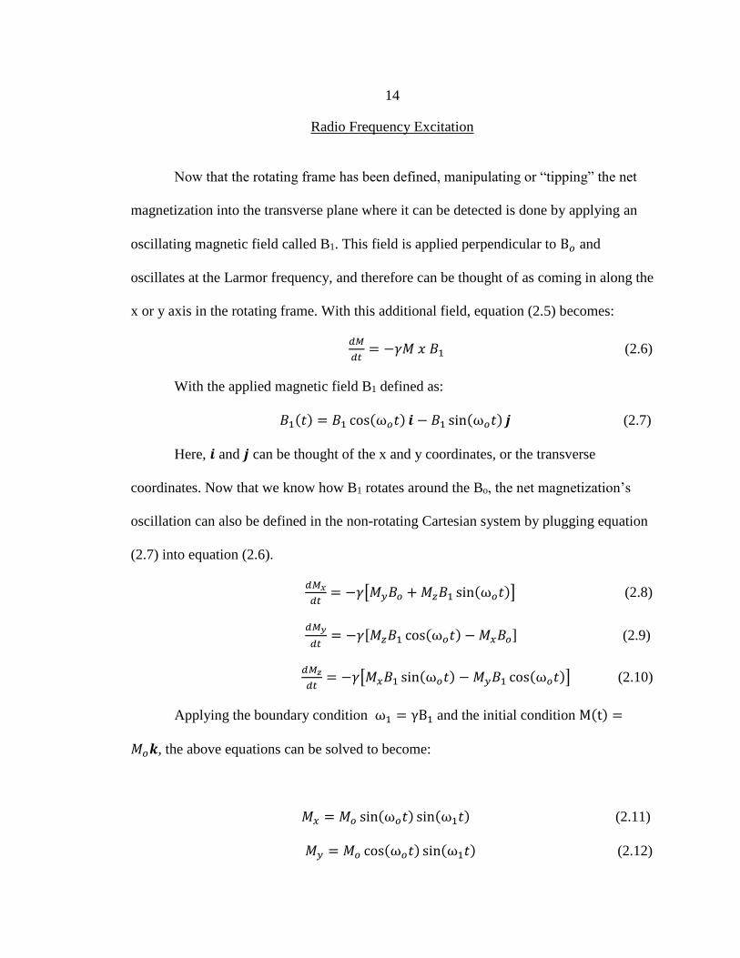
Radio Frequency Excitation

Now that the rotating frame has been defined, manipulating or “tipping” the net

magnetization into the transverse plane where it can be detected is done by applying an

oscillating magnetic field called B1. This field is applied perpendicular to B𝑜 and

oscillates at the Larmor frequency, and therefore can be thought of as coming in along the

x or y axis in the rotating frame. With this additional field, equation (2.5) becomes:

𝑑𝑀

𝑑𝑡= −𝛾𝑀 𝑥 𝐵1 (2.6)

With the applied magnetic field B1 defined as:

𝐵1(𝑡) = 𝐵1 cos(ω𝑜𝑡) 𝒊 − 𝐵1 sin(ω𝑜𝑡) 𝒋 (2.7)

Here, 𝒊 and 𝒋 can be thought of the x and y coordinates, or the transverse

coordinates. Now that we know how B1 rotates around the Bo, the net magnetization’s

oscillation can also be defined in the non-rotating Cartesian system by plugging equation

(2.7) into equation (2.6).

𝑑𝑀𝑥

𝑑𝑡= −𝛾[𝑀𝑦𝐵𝑜 + 𝑀𝑧𝐵1 sin(ω𝑜𝑡)] (2.8)

𝑑𝑀𝑦

𝑑𝑡= −𝛾[𝑀𝑧𝐵1 cos(ω𝑜𝑡) − 𝑀𝑥𝐵𝑜] (2.9)

𝑑𝑀𝑧

𝑑𝑡= −𝛾[𝑀𝑥𝐵1 sin(ω𝑜𝑡) − 𝑀𝑦𝐵1 cos(ω𝑜𝑡)] (2.10)

Applying the boundary condition ω1 = γB1 and the initial condition M(t) =

𝑀𝑜𝒌, the above equations can be solved to become:

𝑀𝑥 = 𝑀𝑜 sin(ω𝑜𝑡) sin(ω1𝑡) (2.11)

𝑀𝑦 = 𝑀𝑜 cos(ω𝑜𝑡) sin(ω1𝑡) (2.12)

15

𝑀𝑧 = 𝑀𝑜 cos(ω1𝑡) (2.13)

These equations show that the net magnetization precesses about B1. In the

rotating frame, the magnetization can be thought of as tipping down into the transverse

plane. It should be noted that the above equations ignore relaxation effects, which are

discussed later [11, 18, 19].

In order to apply the oscillating B1 field that tips the net magnetization into the

transverse plane where signal can be detected, a radio frequency coil is used since the

energy needed to excite spins, between energy states is in the radio frequency range for

large superconducting magnet.

The angle at which the magnetization is tilted is controlled by the duration and

strength of the B1 field termed the radio frequency (rf) pulse, is equation (2.13):

𝛩 = 𝛾𝐵1𝑡𝑝 (2.14)

Where 𝛩 is the tilt angle in degrees, 𝐵1 is the amplitude of the electromagnetic field due

to the rf pulse, and 𝑡𝑝 is the pulse duration.

Figure 2.4: Effect of the rf pulse on the net magnetization

16

A diagram of this action is presented in figure 3.Once the net magnetization is

aligned in the transverse plane it processes, producing a voltage signal referred to as the

Free Induction Decay (FID) [11, 19].

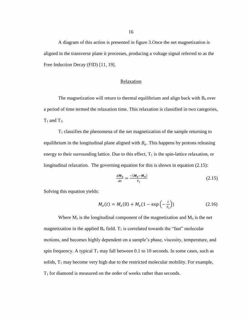
Relaxation

The magnetization will return to thermal equilibrium and align back with Bo over

a period of time termed the relaxation time. This relaxation is classified in two categories,

T1 and T2.

T1 classifies the phenomena of the net magnetization of the sample returning to

equilibrium in the longitudinal plane aligned with 𝐵𝑜. This happens by protons releasing

energy to their surrounding lattice. Due to this effect, T1 is the spin-lattice relaxation, or

longitudinal relaxation. The governing equation for this is shown in equation (2.15):

𝑑𝑴𝑧

𝑑𝑡=

−(𝑴𝒛−𝑴𝒐)

𝑇1 (2.15)

Solving this equation yields:

𝑀𝑧(𝑡) = 𝑀𝑧(0) + 𝑀𝑧(1 − exp (−𝑡

𝑇1)) (2.16)

Where Mz is the longitudinal component of the magnetization and Mo is the net

magnetization in the applied Bo field. T1 is correlated towards the “fast” molecular

motions, and becomes highly dependent on a sample’s phase, viscosity, temperature, and

spin frequency. A typical T1 may fall between 0.1 to 10 seconds. In some cases, such as

solids, T1 may become very high due to the restricted molecular mobility. For example,

T1 for diamond is measured on the order of weeks rather than seconds.

17

A sample’s T1 is generally the restricting parameter when performing

experiments. A rule of thumb within NMR is that pulse sequences must wait 5 T1

intervals before running again to ensure all spins return to equilibrium. Due to this, longer

T1 can increase an experiments time drastically. To combat this, a common relaxation

agent called Magnevist is added to samples which greatly increases the lattice

interactions. Magnevist essentially lowers T1 by creating relaxation sites.

T2 relaxation is dephasing of the net magnetization of hydrogen while in the x-y

plane. It is termed spin-spin relaxation since it is due to energy exchange between spins.

T2 is typically less than T1, and is the governing time restraint on data collection window

for experiments. As described previously, a net magnetization is caused by a state of

phase coherence between spins. Therefore, when these spins start to dephase, or lose

coherence, the net magnetization decreases. A common visualization of T2 is runners on a

race track. At the start of the race, all runners are lined up, but as the race progresses, they

spread out over time. T2 happens very rapidly, especially in porous media where spins

interact with pore walls. Ways to combat this process and collect signal before decay of

the net magnetization will be discussed later. The evolution of the magnetization with T2

is:

𝑑𝑴𝑥,𝑦

𝑑𝑡=

−𝑴𝒙,𝒚

𝑇2 (2.17)

Solving the equation yields:

𝑀𝑥,𝑦(𝑡) = 𝑀𝑥,𝑦(0)𝑒−𝑡/𝑇2 (2.18)

Although ideally the signal decays away purely due to T1 and T2, inhomogenaties in the

magnetic field and/or rf pulses cause additional T2 relaxation. To account for this, the

18

decay of the FID T2 is usually referred to as T2*, meaning that any extra effects on the

relaxation time are contained in the given number [19].

Bloch Equations

Adding the relaxation effects from equations 2.17 and 2.18, to equation 2.5 gives

the Bloch equations, named after their founder physicist Felix Bloch. The result

determines the net magnetization acts when an excitation pulse is applied, and how it

evolves due to both T1 and T2:

𝑑𝑀𝑥

𝑑𝑡= 𝛾𝑀𝑦 (𝐵𝑜 −

𝜔

𝛾) −

𝑀𝑥

𝑇2 (2.19)

𝑑𝑀𝑦

𝑑𝑡= 𝛾𝐵1 − 𝛾𝑀𝑥 (𝐵𝑜 −

𝜔

𝛾) −

𝑀𝑦

𝑇2 (2.20)

𝑑𝑀𝑧

𝑑𝑡= −𝛾𝑀𝑦𝐵1 −

(𝑀𝑧−𝑀𝑜)

𝑇1 (2.21)

Signal Detection

Detecting NMR signal is governed by Faraday’s Law, which predicts how a

magnetic field will interact with an electric circuit to produce an electromagnetic force

(EMF). In this case, the EMF is the result of the processing net magnetization of the

excited protons as they move in the rf coil.

The signal in a NMR experiment is the sum of magnetization, from the ensemble

of spins in the sample. These ensembles can be thought of as groups of hydrogens that

see the same effective gradient within the sample, and therefore will return identical

19

signals back, resulting in one summed signal for all hydrogens within ith ensemble. The

signal (S) for an NMR experiment in a volume element can be defined as:

𝑑𝑆(𝐺, 𝑡) = 𝜌(𝑟)𝑑𝑉𝑒𝑖𝛾𝐵𝑡 (2.22)

where 𝜌(𝑟) at location (𝑟) is defined as the spin density, and 𝑑𝑉is the finite volume

element. These spin ensembles are subject to the thermodynamic principles of

displacement, most notably Brownian motion. Random motions of spins causes

attenuation of S, leading to a Gaussian distribution in displacements once averaged, and

bulk motions are accounted through bulk phase shifts that will be discussed later.

The amplitude of the signal represents the spin density of the sample’s particular

area under measurement. Signal is collected as a function of time, where the amplitude

decays away due to relaxation. To take data into the frequency domain, Fourier

transforms are required. The Fourier relationship between frequency domain (k) and time

domain (t) is:

𝐹(𝑘) = ∫ 𝑓(𝑡)𝑒−𝑖𝑘𝑡𝑑𝑡 (2.24)

𝑓(𝑡) = ∫ 𝐹(𝑘)𝑒𝑖𝑘𝑡𝑑𝑘 (2.25)

Due to the low signal to noise nature of NMR which is best seen in the above

discussion of the Boltzman’s distribution of spins, MR experiments, or sequences, are

commonly repeated many times and averaged to cancel out any noise contained within

the data. This, along with the spin ensemble averaging mentioned in the above paragraph

means that NMR experiments are double averaged, once in space, and again in time. This

double averaging can lead to lengthy experiment times, which varied from 15 minutes, to

24 hours in the experiments performed in this body of work. Due to this, NMR shows

20

many restraints in the measuring of transient or short time dependent systems, and works

much better for steady state and fully developed processes[11, 20].

21

CHAPTER 3: ADVANCED NMR TOPICS: GRADIENTS, SEQUENCES, IMAGING,

AND MOTION TRACKING

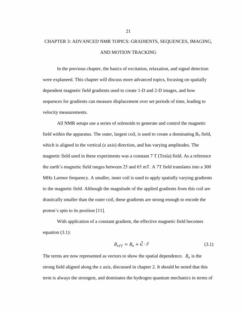
In the previous chapter, the basics of excitation, relaxation, and signal detection

were explaneed. This chapter will discuss more advanced topics, focusing on spatially

dependent magnetic field gradients used to create 1-D and 2-D images, and how

sequences for gradients can measure displacement over set periods of time, leading to

velocity measurements.

All NMR setups use a series of solenoids to generate and control the magnetic

field within the apparatus. The outer, largest coil, is used to create a dominating Bo field,

which is aligned in the vertical (z axis) direction, and has varying amplitudes. The

magnetic field used in these experiments was a constant 7 T (Tesla) field. As a reference

the earth’s magnetic field ranges between 25 and 65 mT. A 7T field translates into a 300

MHz Larmor frequency. A smaller, inner coil is used to apply spatially varying gradients

to the magnetic field. Although the magnitude of the applied gradients from this coil are

drastically smaller than the outer coil, these gradients are strong enough to encode the

proton’s spin to its position [11].

With application of a constant gradient, the effective magnetic field becomes

equation (3.1):

𝐵𝑒𝑓𝑓 = 𝐵𝑜 + �⃗� ∙ 𝑟 (3.1)

The terms are now represented as vectors to show the spatial dependence. 𝐵𝑜 is the

strong field aligned along the z axis, discussed in chapter 2. It should be noted that this

term is always the strongest, and dominates the hydrogen quantum mechanics in terms of

22

spin and Larmor frequency. �⃗� is the applied spatial gradient from the inner coil, and can

be applied in any direction. This term is multiplied by a spatial coordinate, 𝑟, meaning

that the gradient seen by a particular hydrogen ensemble located at one point will see a

different magnitude of gradient than a hydrogen ensemble located at another point in

space.

This additional gradient also changes the frequency of spins as a function of

position with the Larmor frequency relationship, equation (2.1).

𝜔(𝑟) = 𝛾(𝐵𝑒𝑓𝑓) = 𝛾(𝐵𝑜 + �⃗� ∙ 𝑟) (3.2)

As seen above, with the appropriate gradient applications, hydrogen ensembles frequency

can be encoded to its placement in the sample. Gradient applications vary in length,

depending on the desired information from the sample. For example, a simple 2-D image

of an object uses gradients that only encode for space. Gradients can also be used to

measure hydrogen ensemble displacement, which paired with known timings in the

gradient applications can lead to velocity and diffusion measurements. Gradient

applications can even be stacked together in experiments, leading to data that has

multiple dependencies, allowing for experiments such as 2-D velocity images. A few of

these techniques will be discussed later on, mostly focusing on imaging and displacement

techniques used in the body of work for water and WLM flows in porous media.

Slice Selection

This inverse relationship between time and frequency is key to understanding how

rf pulses are applied. To specify a bandwidth, or range of frequencies excited, the length

23

and shape of the rf pulse is adjusted. A long rf pulse will excite a narrow range of

frequencies, and a short r.f pulse will excite a wide range of frequencies. Rf pulses use

adjectives such as hard and soft to quantify the shape of the pulse. Generally, a hard pulse

is square in shape, whereas a soft pulse has a sinc function shape. Along with application

of a gradient, this can selectively excite a slice within the sample.

k-space

As discussed above in chapter 2, the relationship between the time and frequency

domain is what makes NMR imaging possible. This frequency domain is referred to as k-

space, which is the conjugate of position. K-space, is a 2D Fourier transform of a 2-D

image. k’s dependence on a spin’s phase is shown in equation (3.3).

𝑘 =𝛾𝐺𝑡

2𝜋 (3.3)

To collect signal from different points within k-space, gradient sequences are used to

traverse the two dimensions: phase and read, or ky and kx, respectively. The gradients

used to do this are commonly referred to as the read gradient (Gr) and phase gradient

(Gp). A diagram example of how k space is sampled is shown below.

24

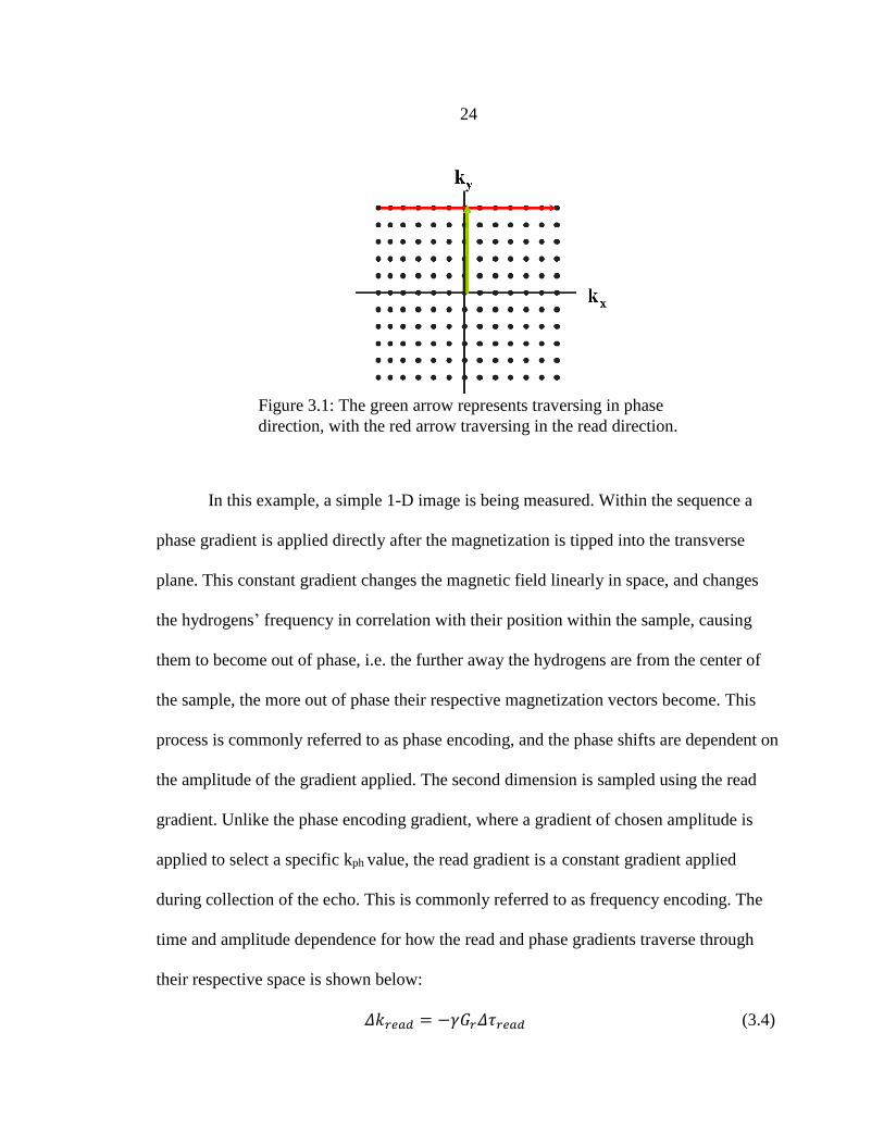
In this example, a simple 1-D image is being measured. Within the sequence a

phase gradient is applied directly after the magnetization is tipped into the transverse

plane. This constant gradient changes the magnetic field linearly in space, and changes

the hydrogens’ frequency in correlation with their position within the sample, causing

them to become out of phase, i.e. the further away the hydrogens are from the center of

the sample, the more out of phase their respective magnetization vectors become. This

process is commonly referred to as phase encoding, and the phase shifts are dependent on

the amplitude of the gradient applied. The second dimension is sampled using the read

gradient. Unlike the phase encoding gradient, where a gradient of chosen amplitude is

applied to select a specific kph value, the read gradient is a constant gradient applied

during collection of the echo. This is commonly referred to as frequency encoding. The

time and amplitude dependence for how the read and phase gradients traverse through

their respective space is shown below:

𝛥𝑘𝑟𝑒𝑎𝑑 = −𝛾𝐺𝑟𝛥𝜏𝑟𝑒𝑎𝑑 (3.4)

Figure 3.1: The green arrow represents traversing in phase

direction, with the red arrow traversing in the read direction.

25

𝛥𝑘𝑝ℎ𝑎𝑠𝑒 = −𝛾𝛥𝐺𝑝𝜏𝑝ℎ𝑎𝑠𝑒 (3.5)

τ represents the time each gradient is applied. Most often in frequency encoding,

kread, is controlled by varying 𝜏𝑟𝑒𝑎𝑑, whereas phase encoding is controlled by varying

either 𝛥𝐺𝑝 or 𝜏𝑝ℎ𝑎𝑠𝑒. A figure of the described sequence is shown below:

Due to the phase space being selected once per sequence, and all read points are

collected within that respected phase line, the time of experiment is highly dependent on

the number of phase lines sampled. The number of phase lines and read lines sampled is

referred to as the resolution, and for a 2-D image the resolution can be thought of as the

same way as a camera or a display screens respective resolution works. Due to the fact

that imaging software used for these experiments takes advantage of Fast Fourier

90°

180°

Gread

Gphas

e

RF

Signal Echo

Figure 3.2: 1-D imaging sequence. Gphase is applied first, with varying

amplitudes each sequence, while Gread is a constant amplitude and applied

during signal collection.

26

Transform (FFT) algorithms, data matrix sizes of 2n are best [11]. A common square 2-D

image may have a matrix size of 256 x 256, which would correspond to 256 phase

encoding lines and 256 read encoding lines, respectively. For oblong shapes, such as a

tube with fluid, an image would most likely be 128 x 256. This is done to keep the pixel

size the same in both directions.

The phase matrix size also varies the length of experiment, which can have high

importance if the sample has any time dependent properties. Because only one line in the

phase direction can be read off in each sequence, a relaxation period must be applied

before the next sequence is run. As mentioned before, 5T1 must pass before the next

sequence can be applied to the sample. Therefore, increasing, or decreasing, the number

of phase lines has a great effect on the length of the experiment. Going from 256 to 128

points in the phase direction will cut the experiment time in half, and can be very useful

when imaging oblong shapes.

To connect the signal collected from sampling k-space in the above sequence, to

the overall goal of imaging, which is finding the spin density at certain position requires a

Fourier transform. This is done by writing equations (2.24) and (2.25) in terms of the

spatial component 𝑟. The resulting equations show the relationship between the signal

gathered, and the spin density in space 𝜌(𝑟):

𝑆(𝑘) = ∫ 𝜌(𝑟) exp[𝑖2𝜋𝑘 ∙ 𝑟] 𝑑𝑟 (3.6)

𝜌(𝑟) = ∫ 𝑆(𝑘) exp[−𝑖2𝜋𝑘 ∙ 𝑟] 𝑑𝑘 (3.7)

27

Motion Tracking: q-space, Diffusion, and Propagators

Much in the same way position is measured using k-space, motion is tracked

using gradient applications in pulse sequences. We similarly call the reciprocal space to

displacement q-space. A good analogy for how bulk motion is tracked in NMR is taking

pictures of fish in water. Imagine standing above the water and taking two pictures,

separated by a time, Δ. When these two pictures are analyzed, it’s seen that the fish has

moved a distance, r-r’. By knowing the distance, and the time between the two pictures, a

velocity can be obtained for that particular fish. Similarly, NMR can track movement by

getting signal from spins at two different times, and knowing the separation between the

two signal acquisitions.

In this body of work, the pulsed gradient stimulated echo experiment (PGStE),

shown in figure 3.3, is used to find effective self-diffusion coefficients, as well as the

overall propagator. This pulse sequence starts with a 90° RF pulse which brings the spins

into the transverse plane. The dephasing gradient pulse winds a helical phase shift the

spin isochromats in the direction of the applied gradient. This square magnetic gradient

pulse is applied for a duration δ, with magnitude 𝑔 in the direction that displacements are

to be measured. Another 90° RF pulse stores the magnetization in the transverse plane,

saving the magnetization from 𝑇2 decay. A spoiler gradient is applied while the

magnetization is in the transverse plane to dephase any remaining signal. The importance

of this is so that the third 90° pulse affects all spin isochromats in the same way, pulling

them again into the transverse plane. This third 90° pulse reverses the direction of

precession of the spin isochromats from their original precession, making the first

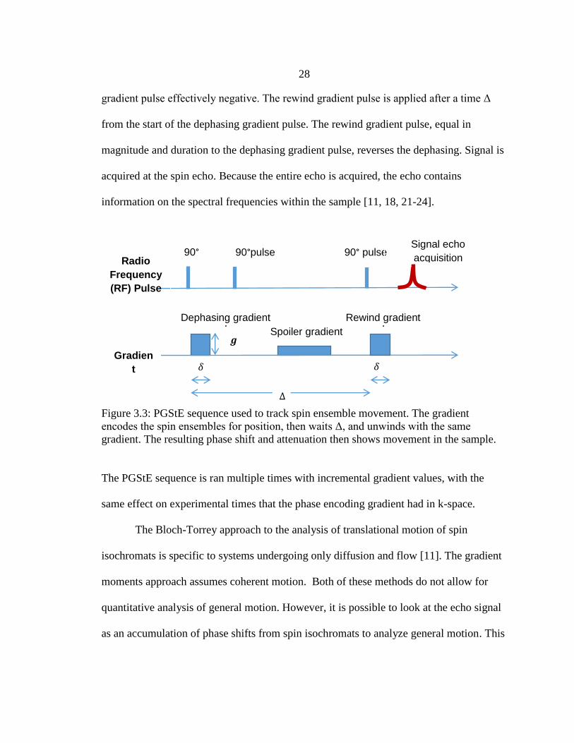
28

gradient pulse effectively negative. The rewind gradient pulse is applied after a time Δ

from the start of the dephasing gradient pulse. The rewind gradient pulse, equal in

magnitude and duration to the dephasing gradient pulse, reverses the dephasing. Signal is

acquired at the spin echo. Because the entire echo is acquired, the echo contains

information on the spectral frequencies within the sample [11, 18, 21-24].

Figure 3.3: PGStE sequence used to track spin ensemble movement. The gradient

encodes the spin ensembles for position, then waits Δ, and unwinds with the same

gradient. The resulting phase shift and attenuation then shows movement in the sample.

The PGStE sequence is ran multiple times with incremental gradient values, with the

same effect on experimental times that the phase encoding gradient had in k-space.

The Bloch-Torrey approach to the analysis of translational motion of spin

isochromats is specific to systems undergoing only diffusion and flow [11]. The gradient

moments approach assumes coherent motion. Both of these methods do not allow for

quantitative analysis of general motion. However, it is possible to look at the echo signal

as an accumulation of phase shifts from spin isochromats to analyze general motion. This

Spoiler gradient

𝒈

Gradien

t

90°pulse 90° pulse Signal echo

acquisition Radio

Frequency

(RF) Pulse

90°

pulse

𝛿

∆

𝛿

Dephasing gradient pulse

Rewind gradient pulse

29

is valid when the narrow gradient pulse approximation can be made, 𝛿 ≪ ∆, such that

spins don’t move considerably over the course of the applied gradient.

𝐸(𝒈, 𝛥) = ∫ 𝜌(𝑟) ∫ 𝑃(𝒓|𝒓′, ∆)exp (𝑖𝛾𝛿𝒈 ∙ [𝒓 − 𝒓′])𝑑𝒓′𝑑𝒓 (3.8)

Equation (3.8) states that the PGSE echo signal, when applying a gradient, g, and using

an observation time, 𝛥, is equal to the sum of all signal phase shifts from all spins due to

displacements from their initial locations 𝒓 to their final locations 𝒓′ over the observation

time

In order to define the signal space in which the propagator is sampled, the

variable 𝒒 is defined: 𝒒 = 𝛾𝛿𝒈. Note that when the finite gradient approximation is

made, 𝒒 is the area under the square gradient pulse in the PGSE experiment. Now,

equation (3.8) can be re-written using the new variable 𝒒.

𝐸(𝒒, 𝛥) = ∫ 𝜌(𝑟) ∫ 𝑃(𝒓|𝒓′, ∆)exp (𝑖𝒒 ∙ [𝒓 − 𝒓′])𝑑𝒓′𝑑𝒓 (3.9)

In equation (3.11), the attenuation only depend on the dynamic displacement: 𝑹 = 𝒓 −

𝒓′. Equation (3.11) can be further simplified by the definition of the average propagator

P :

P (𝑹, 𝑡) = ∫ 𝜌(𝒓)𝑃(𝒓|𝒓 + 𝑹, 𝑡)𝑑𝒓 (3.10)

Equation 3.12 shows that the propagator is the probability that a particle displaces by 𝑅

over the time interval Δ. Applying both of these changes to eq (3.11) yields eq (3.13):

𝐸(𝒒, 𝛥) = ∫ P (𝑹, 𝛥)𝑒𝑥𝑝 (𝑖𝒒 ∙ 𝑹)𝑑𝑹 (3.11)

30

Equation 3.13 displays a Fourier transform relation between the between the echo signal

and the propagator. By probing q-space with the PGSE experiment, spin ensemble

displacements can be found in the form of a propagator, or distribution of displacements.

When there is no bulk flow in the sample equation 3.8 reduces to the Stejskal-

Tanner relation for the attenuation of the echo amplitude [11, 25]:

𝐸(𝑔, ∆) = exp [−𝛾2𝑔2𝛿2𝐷(∆ −𝛿

3)] (3.12)

The Stejskal-Tanner relation shows that the signal attenuation at a certain gradient point

normalized to the zero gradient point is a function of parameters of the pulse sequence,

the gyromagnetic ratio, and the diffusion coefficient. Plotting the signal echo attenuation

of multiple gradient points versus −𝛾2𝑔2𝛿2(∆ −𝛿

3) on a semi-log plot and extracting the

slope, which is the diffusion coefficient, is a very effective method of measuring self-

diffusion coefficients precisely in equilibrated systems. The Stejskal-Tanner method for

finding diffusion coefficients can be used for systems which do not display purely

diffusive motion; for example stochastic motion which changes depending on the

observation time scale, such as restricted diffusion and polymer reputation, and systems

which display stochastic motion due to mixing, such as turbulence and

dispersion[26]][25],. In each of these cases, it is necessary to analyze the diffusion only

over the gradient range which corresponds to 70 to 90 percent of the signal decay. The

reason for this is that the probability of displacements to occur requires higher moments

of the probability distribution function as it moves away from the mean displacement.

Near the mean displacement, the probability of displacement will have Gaussian

characteristics and can be more easily described with the second moment of the

31

probability distribution, which is the mean squared displacement of the molecules and

corresponds with the diffusion coefficient. This will be elaborated on within the

propagator formalism[11, 27, 28].

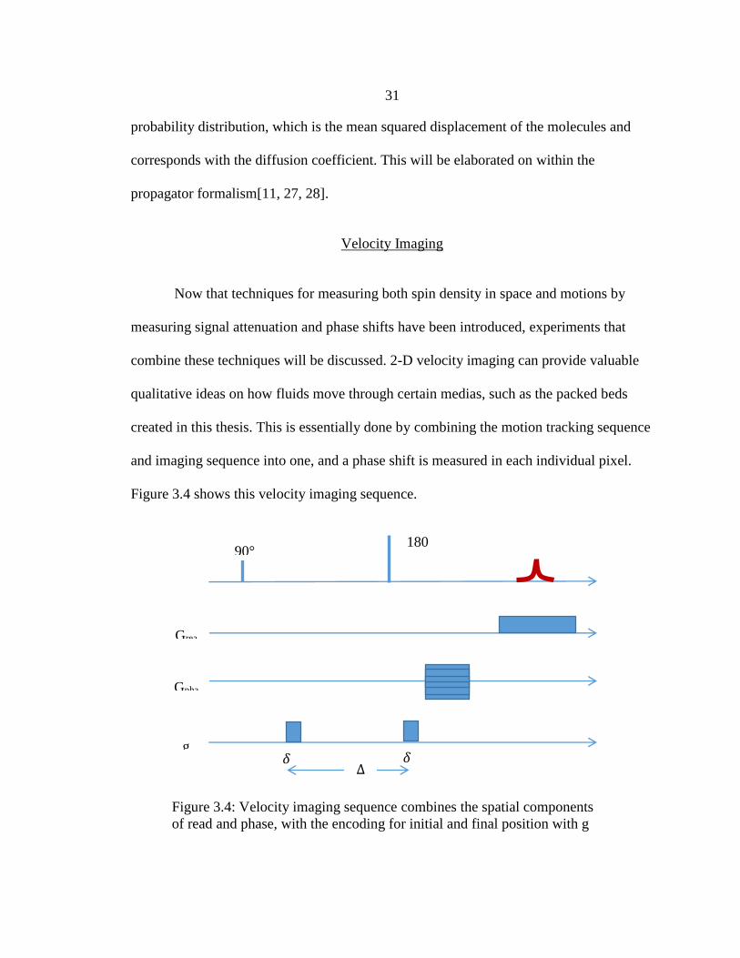
Velocity Imaging

Now that techniques for measuring both spin density in space and motions by

measuring signal attenuation and phase shifts have been introduced, experiments that

combine these techniques will be discussed. 2-D velocity imaging can provide valuable

qualitative ideas on how fluids move through certain medias, such as the packed beds

created in this thesis. This is essentially done by combining the motion tracking sequence

and imaging sequence into one, and a phase shift is measured in each individual pixel.

Figure 3.4 shows this velocity imaging sequence.

90° 180

°

Grea

Gpha

𝛿 𝛿 ∆

g

Figure 3.4: Velocity imaging sequence combines the spatial components

of read and phase, with the encoding for initial and final position with g

32

This velocity sequence leads to a 2-D image in which the phase shift is measured in each

pixel by the following equation:

𝑣 =𝜑2−𝜑1

𝛾(𝑔2−𝑔1)𝛿𝛥 (3.14)

This sequence takes advantage of the basics of both k-space and q-space. It should also

be noted that only two q points are found in each pixel, whereas a normal propagator

usually steps through q space hundreds of times, again in with 2n. Due to spatial

resolution and lower signal to noise in images, higher averaging is usually required, and

therefore 2-D velocity imaging generally takes large amounts of time, and is not useful

for non-steady state flow systems.

33

CHAPTER 4: EXPERIMENTAL SETUP AND METHODS

A Pharmacia P-500 high precision pump was used to circulate fluid through a

high pressure high performance liquid chromatography column (HPLC), with a 10 mm

inner diameter, and a length of 50 mm. The chromatography column was wet packed

with 235 µm, Duke Standards dry polymer microspheres. Fluid was pumped through the

bead pack for at least 12 hours to eliminate air bubbles within the system.

Water experiments were run with 150 mL of deionized water, doped with

Magnevist to reduce T1 relaxation. After 12 hours of flowing, the column was transferred

into the MR system, with the flow going from bottom to top. The flow through system of

pump, tubing, and bead pack used was 40 mL, and was continuously circulated with a

110 mL water basin. Although the MR system has temperature control capability, the

system was not changed from its 21 oC standard setting for water.

For CTAT experiments, approximately 150 mL of de-ionized water was measured

out, and enough Hexadecyltrimethylammonium p-toluenesulfonate dry powder (Sigma

Life Science) was added to create a 10.0 mM solution of CTAT. The solution was placed

in a water bath of 25.0 oC right after the addition of powder, and the solution was stirred

until dissolved then let to rest in the water bath for 24 hours. While keeping the sample

within the water bath, the CTAT solution is pumped into the HPLC bead pack, and

allowed to flow for 12 hours outside the MR system to eliminate air bubbles. The flow

system is then loaded into the MR system, while keeping the solution basin in the water

bath still set at 25 oC. The temperatures of both the surrounding room, and the magnetic

coil, are set to 25 oC.

34

Figure 4.1: Model of entire flow setup while in the NMR magnet for each fluid.

For all solutions, many precautions were taken to avoid air bubbles in the column,

as they cause artifacts in NMR results. All solutions were placed in a vacuum chamber

for 1 hour before being pumped into the system. This was done to try and remove as

much dissolved oxygen from the system that may potentially form air bubbles over time.

Also, the beads were soaked with the fluid solution for several days before the HPLC

column is constructed. This again is done to try and avoid air bubble build up.

For rheology experiments, a TA instruments AR series rheometer with a 2o cone

and plate configuration was used for all solutions. Each solution is mixed for the same

amount of time before measurements as they were for HPLC column loading, and then

pipetted onto the rheometer sample surface. The shear rate is then steadily increased from

10 s-1 to 100 s-1, and viscosity is measured. The sample is covered to help prevent

HPLC

Colum

n

Fluid Temp

control

Pharmacia Pump

NMR Magnet

35

evaporation affecting chemical concentrations during experiments, and the sample is kept

at a constant temperature of 25oC at all times.

NMR measurements used a Bruker AVANCE III spectrometer with a 7 T

superconducting vertical wide bore magnet, Micro2.5 gradient imaging probe with a

maximum gradient of 1.48 T m-1 and 20 mm diameter radiofrequency (rf) coil.

36

CHAPTER 5: RESULTS AND DISCUSSION

Rheology Measurements

Due to CTAT’s ability to combine into cylindrical micelles, complex viscoelastic

behaviors can be observed. Using the AR series rheometer, the viscosity of CTAT at

varying concentrations was tested with increasing shear rates.

Above the CRC, CTAT show’s interesting properties of having shear thickening,

Newtonian, and shear thinning properties depending on applied shear rate. At lower shear

rates, a Newtonian plateau is present. But as shear is increased, CTAT micelles are

becoming larger and more entangled, forming shear induced structures (SIS) that cause

shear thickening[1, 29]. As shear is increased further, the cylindrical micelle structures

start to be pulled apart and align, causing the overall fluid to transfer into a shear thinning

Figure 5.1: Apparent viscosity of CTAT solutions. Concentrations above the critical rodlike

concentration (1.9mM) display a Newtonian plateau, with a shear-thickening regime where

SIS formations occur, followed by a shear thinning regime where structures start to break

down.

37

regime, similar to common polymer fluids. It is important to note that 10 mM CTAT is

the concentration used in all other NMR experiments, due to it having the largest amount

of shear thickening behavior.

To calculate the apparent shear rate found within the bead pack used for MR

experiments, the superficial velocity for 400 mL/hr flowrate was found [9]:

⟨𝑣𝑡𝑢𝑏𝑒⟩ =𝑄

𝐴 (5.1)

where ⟨𝑣𝑡𝑢𝑏𝑒⟩ is the superficial velocity in a tube of equivalent dimensions of the

beadpack, Q is the flowrate, and A is the cross sectional area of the column. Using this,

the pore velocity is found:

⟨𝑣𝑝𝑜𝑟𝑒⟩ =⟨𝑣𝑡𝑢𝑏𝑒⟩

𝜙 (5.2)

where 𝜙 is the porosity of the column. This leads to an average pore velocity of 3.5 mm/s

within each pore. The apparent shear rate in the porous media with spherical beads is

[Bird]:

𝛾𝑎𝑝𝑝 =⟨𝑣𝑝𝑜𝑟𝑒⟩

𝑙=

⟨𝑣𝑝𝑜𝑟𝑒⟩(1−𝜙)

𝑑𝑝𝜙 (5.3)

This leads to an apparent shear rate of 21 s-1 for the flowrate and column used in this

work, which would fall into the Newtonian plateau from figure 5.1. It is important to note

that with a porous media’s complex structure, simple shear conditions do not exist. This

means that the applied shear rate on the fluid is highly dependent on the localized

geometry. Reynolds number and Peclet numbers were also calculated to be 0.001 and

290, respectively.

𝑅𝑒 =𝜌⟨𝑣𝑝𝑜𝑟𝑒⟩𝑙

µ (5.4)

38

𝑃𝑒 =⟨𝑣𝑝𝑜𝑟𝑒⟩𝑙

𝐷𝑜 (5.5)

Where ρ is the fluid density, µ is the viscosity, 𝑙 is the characteristic length of the pore,

and 𝐷𝑜is the self diffusion coefficient.

This means that the fluid is in the laminar regime, and advection is the dominate force

[9, 30].

2D Velocity Images

Two dimensional velocity images were measured for water and 10 mM CTAT

while flowing at 400 mL/hr. Black corresponds to zero velocity, and shows the position

of solid beads, while red corresponds to the fastest velocities. The spatial distribution of

velocities appear to be very similar between the two fluids, with mostly evenly

distributed velocities and a few faster moving pores in red.

Figure 5.2: Cross sectional velocity images of 10 mM CTAT (A) and water (B) flowing

in 10 mm inner diameter porous media with 250 μm beads. Spatial resolution for each

image is 55x55 microns per pixel, with 0.5 mm slice selection. Fluid flowrate was 400

mL/hr, with δ= 0.5 ms, Δ=9.5 ms, gmax= 0.1360 mT/m, 12 mm x 12 mm field of view,

and 256x256 read and phase points.

A B

39

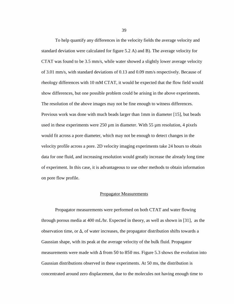
To help quantify any differences in the velocity fields the average velocity and

standard deviation were calculated for figure 5.2 A) and B). The average velocity for

CTAT was found to be 3.5 mm/s, while water showed a slightly lower average velocity

of 3.01 mm/s, with standard deviations of 0.13 and 0.09 mm/s respectively. Because of

rheology differences with 10 mM CTAT, it would be expected that the flow field would

show differences, but one possible problem could be arising in the above experiments.

The resolution of the above images may not be fine enough to witness differences.

Previous work was done with much beads larger than 1mm in diameter [15], but beads

used in these experiments were 250 µm in diameter. With 55 µm resolution, 4 pixels

would fit across a pore diameter, which may not be enough to detect changes in the

velocity profile across a pore. 2D velocity imaging experiments take 24 hours to obtain

data for one fluid, and increasing resolution would greatly increase the already long time

of experiment. In this case, it is advantageous to use other methods to obtain information

on pore flow profile.

Propagator Measurements

Propagator measurements were performed on both CTAT and water flowing

through porous media at 400 mL/hr. Expected in theory, as well as shown in [31], as the

observation time, or Δ, of water increases, the propagator distribution shifts towards a

Gaussian shape, with its peak at the average velocity of the bulk fluid. Propagator

measurements were made with Δ from 50 to 850 ms. Figure 5.3 shows the evolution into

Gaussian distributions observed in these experiments. At 50 ms, the distribution is

concentrated around zero displacement, due to the molecules not having enough time to

40

move. As observation time is increased, the molecules are allowed more time to move,

and the distribution’s peak moves toward a non-zero displacement. It should be noted that

due to the process of random packing of the micro spheres, varying amounts of fluid

would be trapped and not flowing in the porous media. This causes a spike of signal at

the zero displacement point in the propagator.

41

Figure 5.3: Propagator measurements for each observation time for water at 400 mL/hr.

A) and B) show very little Gaussian behavior, but with longer observation times, a

Gaussian shape takes form due to Δ being long enough that the motion has been averaged

over several pore sizes.

0

2

4

6

8

10

-0.5 0 0.5 1 1.5 2

P(Z

,Δ)

Z (mm)

50 ms

0

0.1

0.2

0.3

0.4

0.5

0.6

0.7

-1 0 1 2 3 4

P(Z

,Δ)

Z (mm)

300 ms

0

0.05

0.1

0.15

0.2

0.25

0.3

0.35

-2.5 -0.5 1.5 3.5 5.5 7.5

P(Z

,Δ)

Z (mm)

750 ms

0

0.5

1

1.5

2

2.5

-1 0 1 2 3

P(Z

,Δ)

Z (mm)

100 ms

0

0.05

0.1

0.15

0.2

0.25

0.3

0.35

0.4

0.45

-2 0 2 4 6

P(Z

,Δ)

Z (mm)

500 ms

0

0.1

0.2

0.3

0.4

0.5

-1 1 3 5 7

P(Z

,Δ)

Z (mm)

850 ms

B A

C D

E F

42

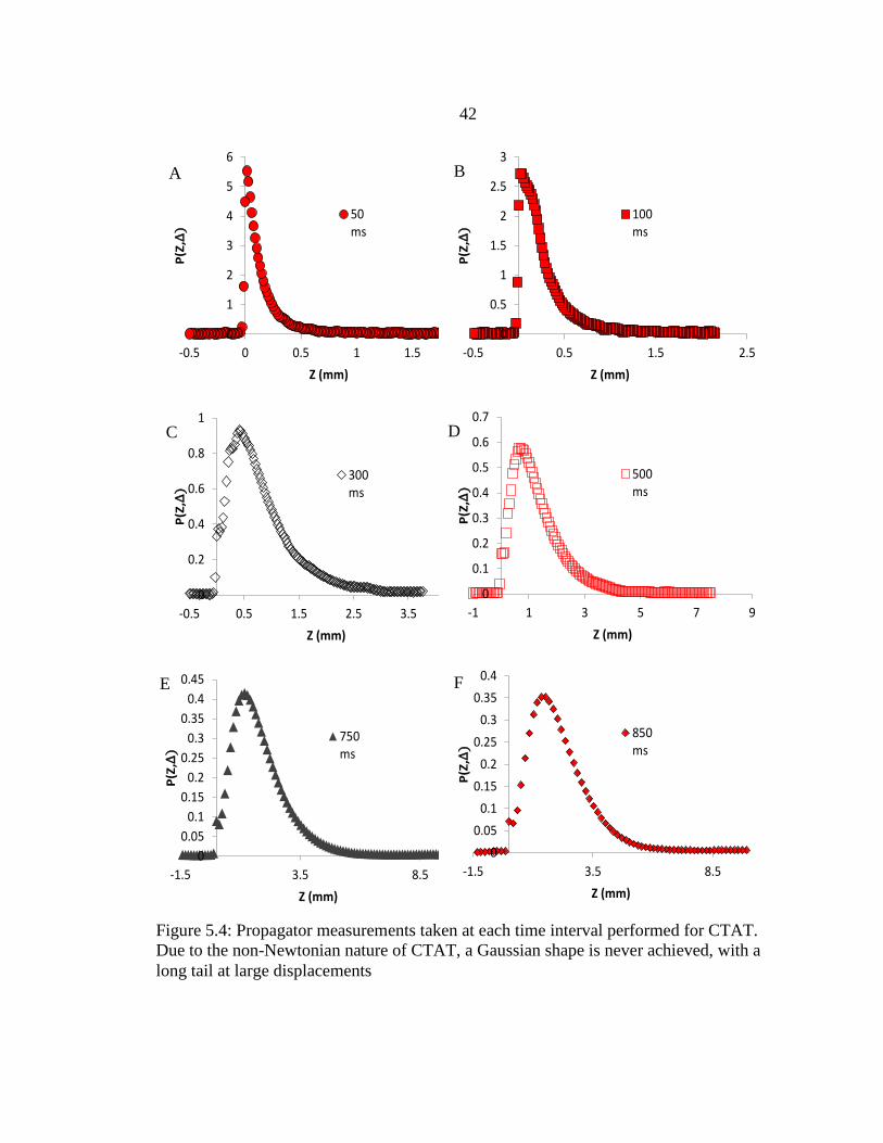
Figure 5.4: Propagator measurements taken at each time interval performed for CTAT.

Due to the non-Newtonian nature of CTAT, a Gaussian shape is never achieved, with a

long tail at large displacements

0

0.05

0.1

0.15

0.2

0.25

0.3

0.35

0.4

0.45

-1.5 3.5 8.5

P(Z

,Δ)

Z (mm)

750ms

0

1

2

3

4

5

6

-0.5 0 0.5 1 1.5 2

P(Z

,Δ)

Z (mm)

50ms

0

0.5

1

1.5

2

2.5

3

-0.5 0.5 1.5 2.5

P(Z

,Δ)

Z (mm)

100ms

0

0.2

0.4

0.6

0.8

1

-0.5 0.5 1.5 2.5 3.5 4.5

P(Z

,Δ)

Z (mm)

300ms

0

0.1

0.2

0.3

0.4

0.5

0.6

0.7

-1 1 3 5 7 9

P(Z

,Δ)

Z (mm)

500ms

A B

C D

E

0

0.05

0.1

0.15

0.2

0.25

0.3

0.35

0.4

-1.5 3.5 8.5

P(Z

,Δ)

Z (mm)

850ms

F

43

For CTAT, the evolution to a steady state shape is much slower, and long

displacement tails can be seen as early as 300 ms. This is evidence that although the bulk

of the fluid is moving at slower velocities, some pores are experiencing significantly

higher velocities [15]. Both fluids are moving at the same volumetric flow rate, with the

same cross sectional area in the column, but CTAT shows a much different distribution

of displacements. Comparisons of these two fluids can be seen below.

Figure 5.5: Propagator measurements. Propagator measurements. (A) CTAT for all Δ. (B)

Water for all Δ. (C) CTAT for Δ= 300, 500, and 850 ms. (D) Water for Δ= 300, 500, and

850 ms.. Water shows an evolution towards a Gaussian shape at longer observation times,

whereas CTAT shows an evolution towards a non-Gaussian shape with longer tails.

A B

C D

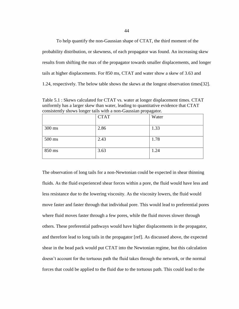
44

To help quantify the non-Gaussian shape of CTAT, the third moment of the

probability distribution, or skewness, of each propagator was found. An increasing skew

results from shifting the max of the propagator towards smaller displacements, and longer

tails at higher displacements. For 850 ms, CTAT and water show a skew of 3.63 and

1.24, respectively. The below table shows the skews at the longest observation times[32].

Table 5.1 : Skews calculated for CTAT vs. water at longer displacement times. CTAT

uniformly has a larger skew than water, leading to quantitative evidence that CTAT

consistently shows longer tails with a non-Gaussian propagator.

The observation of long tails for a non-Newtonian could be expected in shear thinning

fluids. As the fluid experienced shear forces within a pore, the fluid would have less and

less resistance due to the lowering viscosity. As the viscosity lowers, the fluid would

move faster and faster through that individual pore. This would lead to preferential pores

where fluid moves faster through a few pores, while the fluid moves slower through

others. These preferential pathways would have higher displacements in the propagator,

and therefore lead to long tails in the propagator [ref]. As discussed above, the expected

shear in the bead pack would put CTAT into the Newtonian regime, but this calculation

doesn’t account for the tortuous path the fluid takes through the network, or the normal

forces that could be applied to the fluid due to the tortuous path. This could lead to the

CTAT Water

300 ms 2.86 1.33

500 ms 2.43 1.78

850 ms 3.63 1.24

45

fluid going through a large array of shear rates in the porous media, and measurements

for CTAT could come from Newtonian, shear thickening, and/or shear thinning

regime[33, 34] [35, 36].

Dispersion Measurements

To help further quantify the non-Gaussian nature of CTAT, the approach of

Guillon et al [37] was to measure dispersion. A criteria of Δ above 1.22 seconds was used

to make sure all of the pore space is sampled, as measurements need to be in the

asymptotic regime. This was found by using the criteria:

√2𝐷𝑜𝑡 > 0.3𝑑𝑔 (5.4)

Where 𝐷𝑜 is the self-diffusion coefficient and 𝑑𝑔 is the bead diameter. Experiments of Δ

varying from 1.3 ms to 1.9 ms were run to analyze dispersion within the bead pack for

both fluids. Collection techniques similar to the Stejskal-Tanner relation were used, but

the attenuation q-space data was analyzed [25] [11]. Q-space, and not displacement, was

analyzed to avoid any problems that could occur with fourier transforming the data. In

the asymptotic and Gaussian regime, standard deviation of the displacement, or the

variance of displacement, scales linearly with observation time. Sub, or super dispersion

is characterized with a power law scaling[37, 38].

𝜎2 ∝ Δα (5.5)

To find the relationship between signal and variance, equation (3.9) is modified to give:

ln|𝐸(𝑞, 𝛥)| = −1

2𝜎2𝑞2 (5.6)

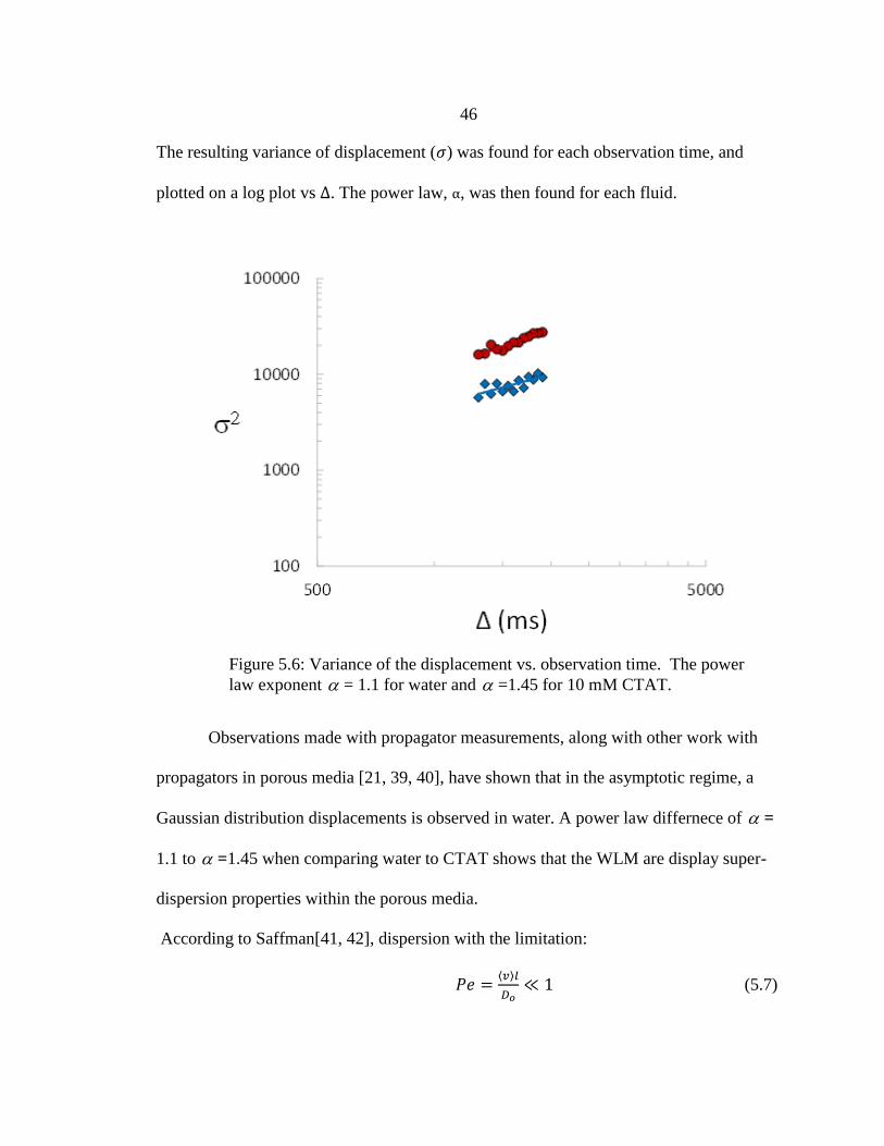
46

The resulting variance of displacement (𝜎) was found for each observation time, and

plotted on a log plot vs Δ. The power law, α, was then found for each fluid.

Observations made with propagator measurements, along with other work with

propagators in porous media [21, 39, 40], have shown that in the asymptotic regime, a

Gaussian distribution displacements is observed in water. A power law differnece of =

1.1 to =1.45 when comparing water to CTAT shows that the WLM are display super-

dispersion properties within the porous media.

According to Saffman[41, 42], dispersion with the limitation:

𝑃𝑒 =⟨𝑣⟩𝑙

𝐷𝑜≪ 1 (5.7)

Figure 5.6: Variance of the displacement vs. observation time. The power

law exponent = 1.1 for water and =1.45 for 10 mM CTAT.

47

follows Taylor dispersion, where longitudinal dispersion is increased with shear in flow.

Pe scales with dispersion by a power law Peβ, where β=1 for situations in which velocity

variations cause dispersive effects, and β=2 for diffusion being the dominant effects [43].

For CTAT, in which transport in the porous media is anomalous compared to water, Pe

number scaling would be very difficult to predict due to WLM changing the dispersive

forces acting upon the fluid[44-47].

Conclusion

Data collected from 2-D velocity images showed slight evidence of flow profile

changing when comparing water to CTAT, but by using PGSE NMR, changes were

witnessed by measuring displacements of spin isochromats. Propagator measurements,

along with measured skew, showed that CTAT displays a non-Gaussian distribution, with

long tails in higher displacements. Dispersion experiments showed that non-Gaussian

CTAT changes the power law scaling from Gaussian scaling in 𝜎 vs Δ when experiments

are analyzed in the non-Fourier transformed q-space.

This gives a small amount of insight into how WLM’s complex rheological

properties change the fluid’s transport in porous media. Much more experimentation is

needed to fully understand the mechanisms by which the WLM’s cause non-Gaussian

behavior, and how it can be tied to the fluid rheology.

48

REFERENCES

1. Yang, J., Viscoelastic wormlike micelles and their applications. Current Opinion

in Colloid & Interface Science, 2002. 7(5-6): p. 276-281.

2. Maitland, G.C., Oil and gas production. Current Opinion in Colloid & Interface

Science, 2000. 5(5-6): p. 301-311.

3. Kamari, A., et al., Reliable method for the determination of surfactant retention in

porous media during chemical flooding oil recovery. Fuel, 2015. 158: p. 122-128.

4. Seymour, J.D. and P.T. Callaghan, Generalized approach to NMR analysis of

flow and dispersion in porous media. Aiche Journal, 1997. 43(8): p. 2096-2111.

5. Seymour, J.D., et al., Magnetic resonance microscopy of biofouling induced scale

dependent transport in porous media. Advances in Water Resources, 2007. 30(6-

7): p. 1408-1420.

6. Yang, J., Viscoelastic wormlike micelles and their applications. Current Opinion

in Colloid & Interface Science, 2002: p. 276-281.

7. Moss, G.R. and J.P. Rothstein, Flow of wormlike micelle solutions past a confined

circular cylinder. Journal of Non-Newtonian Fluid Mechanics, 2010. 165(21-22):

p. 1505-1515.

8. Chu, Z., C.A. Dreiss, and Y. Feng, Smart wormlike micelles. Chem Soc Rev,

2013. 42(17): p. 7174-203.

9. R. Byron Bird, W.E.S., Edwin N. Lightfoot, Transport Phenomena. 2007, New

York: J. Wiley.

10. Balhoff, M.T. and K.E. Thompson, A macroscopic model for shear-thinning flow

in packed beds based on network modeling. Chemical Engineering Science, 2006.

61(2): p. 698-719.

11. Callaghan, P.T., Translational Dynamics & Magnetic Resonance. 2011, New

York: Oxford University Press.

12. Chhabra, R.P., J. Comiti, and I. Machac, Flow of non-Newtonian fluids in fixed

and fluidised beds. Chemical Engineering Science, 2001. 56(1): p. 1-27.

13. Maier, R.S., et al., Pore-scale simulation of dispersion. Physics of Fluids, 2000.

12(8): p. 2065-2079.

49

14. Koch, D.L. and J.F. Brady, Dispersion in Fixed-Beds. Journal of Fluid

Mechanics, 1985. 154(May): p. 399-427.

15. Mertens, D., et al., Newtonian and non-Newtonian low Re number flow through

bead packings. Chemical Engineering & Technology, 2006. 29(7): p. 854-861.

16. Muller, M., J. Vorwerk, and P.O. Brunn, Optical studies of local flow behaviour

of a non-Newtonian fluid inside a porous medium. Rheologica Acta, 1998. 37(2):

p. 189-194.

17. Pearson, J.R.A. and P.M.J. Tardy, Models for flow of non-Newtonian and complex

fluids through porous media. Journal of Non-Newtonian Fluid Mechanics, 2002.

102(2): p. 447-473.

18. Hinshaw, W.S. and A.H. Lent, An Introduction to Nmr Imaging - from the Bloch

Equation to the Imaging Equation. Proceedings of the Ieee, 1983. 71(3): p. 338-

350.

19. Hahn, E.L., Spin echoes. Phys Rev E Stat Phys Plasmas Fluids Relat Interdiscip

Topics, 1950. 77: p. 746.

20. Ernst, R.R., G. Bodenhausen, and A. Wokaun, Principles of Nuclear Magnetic

Resonance in One and Two Dimensions. 1988: Oxford University Press.

21. Seymour, J.D. and P.T. Callaghan, ''Flow-diffraction'' structural characterization

and measurement of hydrodynamic dispersion in porous media by PGSE NMR.

Journal of Magnetic Resonance Series A, 1996. 122(1): p. 90-93.

22. Callaghan, P.T., S. Godefroy, and B.N. Ryland, Diffusion-relaxation correlation

in simple pore structures. Journal of Magnetic Resonance, 2003. 162(2): p. 320-

327.

23. Manz, B., L.F. Gladden, and P.B. Warren, Flow and dispersion in porous media:

Lattice-Boltzmann and NMR studies. Aiche Journal, 1999. 45(9): p. 1845-1854.

24. Manz, B., P. Alexander, and L.F. Gladden, Correlations between dispersion and

structure in porous media probed by nuclear magnetic resonance. Physics of

Fluids, 1999. 11(2): p. 259-267.

25. Stejskal, E.O. and J.E. Tanner, Spin Diffusion Measurements: Spin Echoes in the

Presence of a Time-Dependent Field Gradient. Journal of Chemical Physics,

1965. 42(1): p. 288-+.

50

26. Callaghan, P.T. and A. Coy, Evidence for Reptational Motion and the

Entanglement Tube in Semidilute Polymer-Solutions. Physical Review Letters,

1992. 68(21): p. 3176-3179.

27. Callaghan, P.T., et al., Diffusion in Porous Systems and the Influence of Pore

Morphology in Pulsed Gradient Spin-Echo Nuclear-Magnetic-Resonance Studies.

Journal of Chemical Physics, 1992. 97(1): p. 651-662.

28. Hunter, M.W. and P.T. Callaghan, NMR measurement of nonlocal dispersion in

complex flows. Phys Rev Lett, 2007. 99(21): p. 210602.

29. Rojas, M.R., A.J. Muller, and A.E. Saez, Shear rheology and porous media flow

of wormlike micelle solutions formed by mixtures of surfactants of opposite

charge. J Colloid Interface Sci, 2008. 326(1): p. 221-6.

30. Bear, J., Dynamics of Fluids in Porous Media. 1972, New York: Dover

Publication.

31. Seymour, J.D.a.P.T.C., Generalized approach to NMR analysis of flow and

dispersion in porous medium. AIChE Journal, 1997. 43: p. 2096-2111.

32. Doane, D.P. and L.E. Seward, Measuring Skewness: A Forgotten Statistic?

Journal of Statistics Education, 2011. 19(2).

33. Prudhomme, R.K. and G.G. Warr, Elongational Flow of Solutions of Rodlike

Micelles. Langmuir, 1994. 10(10): p. 3419-3426.

34. Fischer, P., G.G. Fuller, and Z.C. Lin, Branched viscoelastic surfactant solutions

and their response to elongational flow. Rheologica Acta, 1997. 36(6): p. 632-

638.

35. Gonzalez, J.M., et al., The role of shear and elongation in the flow of solutions of

semi-flexible polymers through porous media. Rheologica Acta, 2005. 44(4): p.

396-405.

36. Chevalier, T., et al., Breaking of non-Newtonian character in flows through a

porous medium. Physical Review E, 2014. 89(2).

37. Guillon, V., et al., Superdispersion in homogeneous unsaturated porous media

using NMR propagators. Physical Review E, 2013. 87(4).

38. Guillon, V., et al., Computing the Longtime Behaviour of NMR Propagators in

Porous Media Using a Pore Network Random Walk Model. Transport in Porous

Media, 2014. 101(2): p. 251-267.

51

39. Khrapitchev, A.A. and P.T. Callaghan, Reversible and irreversible dispersion in a

porous medium. Physics of Fluids, 2003. 15(9): p. 2649-2660.

40. Amin, M.H.G., et al., Study of flow and hydrodynamic dispersion in a porous

medium using pulsed-field-gradient magnetic resonance. Proceedings of the

Royal Society a-Mathematical Physical and Engineering Sciences, 1997.

453(1958): p. 489-513.

41. Saffman, P.G., A Theory of Dispersion in a Porous Medium. Journal of Fluid

Mechanics, 1959. 6(3): p. 321-349.

42. Saffman, P.G., Dispersion Due to Molecular Diffusion and Macroscopic Mixing

in Flow through a Network of Capillaries. Journal of Fluid Mechanics, 1960.

7(2): p. 194-208.

43. Salles, J., et al., Taylor Dispersion in Porous-Media - Determination of the

Dispersion Tensor. Physics of Fluids a-Fluid Dynamics, 1993. 5(10): p. 2348-

2376.

44. Chaplane, V., C. Allain, and J.P. Hulin, Tracer dispersion in power law fluids

flow through porous media: Evidence of a cross-over from a logarithmic to a

power law behaviour. European Physical Journal B, 1998. 6(2): p. 225-231.

45. Codd, S.L., et al., Taylor dispersion and molecular displacements in Poiseuille

flow. Phys Rev E Stat Phys Plasmas Fluids Relat Interdiscip Topics, 1999. 60(4 Pt

A): p. R3491-4.

46. Metzler, R. and J. Klafter, The random walk's guide to anomalous diffusion: a

fractional dynamics approach. Physics Reports-Review Section of Physics

Letters, 2000. 339(1): p. 1-77.

47. Sullivan, S.P., L.F. Gladden, and M.L. Johns, Simulation of power-law fluid flow

through porous media using lattice Boltzmann techniques. Journal of Non-

Newtonian Fluid Mechanics, 2006. 133(2-3): p. 91-98.