Nuclear magnetic relaxation by the dipolar EMOR … · analytical results for integral relaxation...

THE JOURNAL OF CHEMICAL PHYSICS 144, 084202 (2016)

Nuclear magnetic relaxation by the dipolar EMOR mechanism:General theory with applications to two-spin systems

Zhiwei Chang and Bertil Hallea)

Division of Biophysical Chemistry, Department of Chemistry, Lund University, P.O. Box 124,SE-22100 Lund, Sweden

(Received 6 January 2016; accepted 3 February 2016; published online 25 February 2016)

In aqueous systems with immobilized macromolecules, including biological tissue, the longitudinalspin relaxation of water protons is primarily induced by exchange-mediated orientational randomi-zation (EMOR) of intra- and intermolecular magnetic dipole-dipole couplings. We have embarkedon a systematic program to develop, from the stochastic Liouville equation, a general and rigoroustheory that can describe relaxation by the dipolar EMOR mechanism over the full range of exchangerates, dipole coupling strengths, and Larmor frequencies. Here, we present a general theoreticalframework applicable to spin systems of arbitrary size with symmetric or asymmetric exchange.So far, the dipolar EMOR theory is only available for a two-spin system with symmetric exchange.Asymmetric exchange, when the spin system is fragmented by the exchange, introduces new andunexpected phenomena. Notably, the anisotropic dipole couplings of non-exchanging spins break theaxial symmetry in spin Liouville space, thereby opening up new relaxation channels in the locallyanisotropic sites, including longitudinal-transverse cross relaxation. Such cross-mode relaxationoperates only at low fields; at higher fields it becomes nonsecular, leading to an unusual invertedrelaxation dispersion that splits the extreme-narrowing regime into two sub-regimes. The generaldipolar EMOR theory is illustrated here by a detailed analysis of the asymmetric two-spin case,for which we present relaxation dispersion profiles over a wide range of conditions as well asanalytical results for integral relaxation rates and time-dependent spin modes in the zero-field andmotional-narrowing regimes. The general theoretical framework presented here will enable a quan-titative analysis of frequency-dependent water-proton longitudinal relaxation in model systems withimmobilized macromolecules and, ultimately, will provide a rigorous link between relaxation-basedmagnetic resonance image contrast and molecular parameters. C 2016 Author(s). All article content,except where otherwise noted, is licensed under a Creative Commons Attribution (CC BY) license(http://creativecommons.org/licenses/by/4.0/). [http://dx.doi.org/10.1063/1.4942026]

I. INTRODUCTION

Soft-tissue contrast in clinical magnetic resonanceimaging derives largely from spatial variations in therelaxation behavior of water protons. Yet, a rigorous theoryrelating the water 1H relaxation rate to microscopic parametersis still not available. The lack of theoretical underpinningis also a limitation in biophysical studies of, for example,water-protein interactions and intermittent protein dynamicsby field-cycling measurements of the water 1H magneticrelaxation dispersion (MRD) in protein gels. Previously,such data have been interpreted with semi-phenomenologicalmodels1–3 involving questionable assumptions about therelaxation-inducing motions.4,5 Earlier water 1H MRD studiesof biopolymer gels from this laboratory5,6 made use of anonrigorous extension of the multi-spin Solomon equations toconditions outside the motional-narrowing regime.

Nuclear spins residing permanently in immobilizedmacromolecules give rise to solid-state type NMR spectra,whereas spins that are only transiently associated withthe macromolecules, because they exchange chemically or

a)[email protected]

physically with the solvent phase, exhibit liquid-state NMRproperties provided that the immobilized macromoleculesare isotropically distributed so that anisotropic nuclearspin couplings are averaged to zero. In such locallyanisotropic samples, exchange plays a dual role. On theone hand, exchange transfers magnetizations and coherencesbetween macromolecule-bound spins and solvent spins. Onthe other hand, exchange randomizes the orientation ofanisotropic nuclear interaction tensors, thereby inducingspin relaxation. For this relaxation mechanism, known asexchange-mediated orientational randomization (EMOR), themotional-narrowing regime coincides with the fast-exchangeregime. For the EMOR mechanism, the conventional Bloch-Wangsness-Redfield (BWR) perturbation theory of nuclearspin relaxation7 breaks down when, as is frequently the case,the mean survival time of the macromolecule-bound spin iscomparable to, or longer than, the inverse of the anisotropicnuclear spin coupling that it experiences in the bound state. Wehave therefore embarked on a program to develop a generalnon-perturbative theory, based on the stochastic Liouvilleequation (SLE),8,9 that can describe relaxation by the EMORmechanism over the full range of exchange rates and spincoupling strengths.

0021-9606/2016/144(8)/084202/16 144, 084202-1 © Author(s) 2016.

Reuse of AIP Publishing content is subject to the terms: https://publishing.aip.org/authors/rights-and-permissions. Downloaded to IP: 130.235.252.19 On: Thu, 25 Feb

2016 19:26:38

http://dx.doi.org/10.1063/1.4942026

http://dx.doi.org/10.1063/1.4942026

http://creativecommons.org/licenses/by/4.0/











































http://dx.doi.org/10.1063/1.4942026

http://dx.doi.org/10.1063/1.4942026

http://dx.doi.org/10.1063/1.4942026

http://dx.doi.org/10.1063/1.4942026

http://dx.doi.org/10.1063/1.4942026

http://dx.doi.org/10.1063/1.4942026

http://dx.doi.org/10.1063/1.4942026

http://dx.doi.org/10.1063/1.4942026

mailto:[email protected]






















http://crossmark.crossref.org/dialog/?doi=10.1063/1.4942026&domain=pdf&date_stamp=2016-02-25

084202-2 Z. Chang and B. Halle J. Chem. Phys. 144, 084202 (2016)

The EMOR SLE theory was first developed forquadrupolar relaxation10,11 and it has been extensively appliedto water 2H MRD studies of colloidal silica,12 polymergels,13,14 cross-linked proteins,15–18 and cells.19 As comparedto quadrupolar relaxation, which only involves single spins,dipolar relaxation is theoretically more challenging. TheEMOR SLE theory for dipolar relaxation of a homonuclearspin pair exchanging as a unit20 is isomorphic with thecorresponding theory for quadrupolar relaxation of a singlespin-1,11 but for heteronuclear spins, multispin (>2) systemsand/or fragmentation of the spin system by exchange,qualitatively new phenomena appear in the dipolar relaxation.In a previous report,20 hereafter referred to as Paper I, wedeveloped the EMOR SLE theory for a (homonuclear orheteronuclear) spin pair that exchanges as an intact unit, asituation that we now refer to as symmetric exchange. Contraryto our earlier expectations,20 the case of asymmetric exchange,where only one of the two dipole-coupled spins undergoesexchange, differs fundamentally from the symmetric case. Inparticular, since the non-exchanging spins are not isotropicallyaveraged, the longitudinal and transverse magnetizations aredynamically coupled in the anisotropic sites. Such cross-moderelaxation, distinct from the cross-spin relaxation familiarfrom the Solomon equations,21 gives rise to an invertedrelaxation dispersion at low field.

Here, we develop the general dipolar EMOR SLE theory,valid for spin systems of arbitrary size and for symmetric aswell as asymmetric exchange. To illustrate the general theory,we present explicit results for the asymmetric two-spin case,which is contrasted with the previously treated symmetrictwo-spin case.20 These results are directly applicable to, forexample, a macromolecular hydroxyl proton in chemicalexchange with water protons (asymmetric case) or to aninternal water molecule in physical exchange with bulk water(symmetric case).

This paper is organized as follows. In Sec. II, we presentthe dipolar EMOR formalism for an arbitrary spin system,with general and two-spin results in separate subsections. Ascompared to Paper I, the formalism has been modified andextended in order to accommodate asymmetric exchange.In Sec. III, we discuss the zero-field regime, which isof special significance for asymmetric exchange, and themotional-narrowing regime, where we obtain explicit resultsfor the asymmetric two-spin case that serve to rationalizethe unexpected inverted relaxation dispersion. In Sec. IV, weillustrate the theory by numerical results for the two-spin case,emphasizing the new phenomena that emerge for asymmetricexchange. Further physical insight is provided by an analysisof the time evolution of the relevant spin modes. Lengthyderivations and tables are relegated to six appendices.22

II. DIPOLAR EMOR THEORY

A. Spin systems and exchange cases

1. General case

We consider a system of spin-1/2 nuclei, some or all ofwhich exchange between a solid-like anisotropic (A) state anda liquid-like bulk (B) state. The spins need not be isochronous

(or even homonuclear), but the Zeeman coupling is taken tobe the same in states A and B. (In any case, longitudinalrelaxation is not affected by exchange-modulation of theZeeman coupling.) The A state comprises a large number, N ,of sites distinguished by their fixed orientations. Collectively,the N site orientations approximate an isotropic distribution.Each A site hosts a spin system with mA ≥ 2 mutually dipole-coupled spins. A subset (or fragment) of this spin system,comprising mB spins (with 1 ≤ mB ≤ mA), exchanges with theB state. The exchange is said to be symmetric if mB = mAand asymmetric if mB < mA. We refer to the mB exchangingspins as labile spins and the mA − mB nonexchanging spins asnonlabile. The general theory developed here is valid withoutfurther restrictions on mA and mB.

To identify different exchange cases, we use the notation“(spins in state A)–(spins in state B).” For example, IS–Iis a two-spin system with one labile spin and ISP–IS is athree-spin system with two labile spins. The IS–I case mightrefer to a macromolecular hydroxyl proton (I) dipole-coupledto a nearby aliphatic proton (S). The ISP–IS case mightrefer to the two protons (IS) of a water molecule temporarilytrapped in a protein cavity, where the water protons aredipole-coupled to a nearby aliphatic proton (P). Note thatboth of these cases involve asymmetric exchange since thespin system is fragmented, even though no covalent bonds arebroken in the latter case. We shall only consider cases wherea single type of spin system is present in each state, but wenote that it is straightforward to extend the theory to caseswhere more than one subset of spins exchange independently,possibly at different rates.

The orientations of all internuclear vectors involving atleast one labile spin are taken to be instantaneously random-ized upon exchange, thereby inducing dipolar relaxation. Thisassumption in the EMOR model is justified if the meansurvival time of the labile spin(s) in the A sites is longcompared to the time required for orientational randomizationwhen the labile spin(s) has been transferred to state B. Thisis the case, for example, for chemical exchange of labilemacromolecular protons with bulk water and for physicalexchange of trapped (internal) water molecules with bulkwater.20,23 We can then ignore all dipole couplings among thelabile spins in state B. If so desired, the small and frequency-independent relaxation contribution from fast modulation ofdipole couplings in state B can be added to the final expressionfor the overall relaxation rate.20

At any time, a fraction PA of the labile spins reside instate A, while a fraction PB = 1 − PA reside in state B. Thenonlabile spins are only present in state A. The general dipolarEMOR theory developed here is valid without restrictions onPA. However, some of our results are only valid in the diluteregime, where PA ≪ 1. In most applications of interest, thisinequality is satisfied with a wide margin.4–6

2. Two-spin case

In Paper I, we analyzed the symmetric exchangecase IS–IS. Here, we consider the more complicated andinteresting asymmetric exchange case IS–I. In a typicalapplication, spin I is a labile proton, e.g., in a hydroxyl


2016 19:26:38


group, exchanging with bulk water protons. This is actuallyan IS–I2 case, but since the I–I dipole coupling in state Bplays no role (see above), the results are the same as forthe IS–I case. The only difference between the IS–I andIS–I2 cases lies in the interpretation of the I-spin fraction:PA(IS–I2) = PA(IS–I)/[2 − PA(IS–I)].

The Zeeman (HZ) and dipolar (HD) Hamiltonians forthe two-spin system are given by Eqs. (2.2) and (2.3)of Paper I, with the dipole frequency ωD defined as3/2 times the usual dipole coupling constant, i.e., ωD≡ (3/2) [µ0/(4π)] γIγS ~/r 3

I S.

B. Composite Liouville space

1. General case

Formally, we can regard the total system as a mixtureof N + 1 species, labeled by α = 0, 1, 2, . . . ,N , with α = 0referring to state B and α ≥ 1 to site α in state A. Thus, P0 = PBand Pα = PA/N for α ≥ 1. All spin systems belonging to agiven species α have the same spin Hamiltonian Hα, withH0 = HZ for α = 0 and Hα = HZ + Hα

D for α ≥ 1.To an excellent approximation, the individual spin

systems can be regarded as mutually noninteracting anduncorrelated. The spin density operator of the total system thenreduces to a direct sum of species spin density operators σα,each of which represents an ensemble of spin systems in siteα.24–26 In the absence of exchange, the spin systems associatedwith the N + 1 species evolve independently according to theLiouville equation

ddt

σα(t) = − i Lα σα(t). (1)

The Liouville-space representation σα of the species densityoperator σα is a column vector of dimension Dα = 22 mα − 1,where mα (=mA or mB) is the number of spins in species α and−1 comes from omitting the superfluous identity basis operator.

The spin density operator of the total system is representedas a column vector in a composite Liouville space24,25 ofdimension D = DB + DAN , formed as the direct sum of thespin operator spaces of the N + 1 species. Thus,

σ =

σ0

σ1

...

σN

and σα =

σα1...

σαDα

. (2)

An element of the D-dimensional column vector σ can beexpressed in the following equivalent ways:

σαnα= (nα |σα) = TrB†nασ

α = TrB†nα ⟨α|σ⟩=α|σnα

= ⟨α|(nα |σ)⟩ = α,nα |σ, (3)

where Bnα is a member of a complete set of orthonormal spinbasis operators for species α,

(Bnα |Bpα) = TrB†nαBpα = δnαpα. (4)

To make full use of symmetry, we represent spin Liouvillespace in a basis of irreducible spherical tensor operators

(ISTOs) TKQ (λ) of rank K , quantum order Q, and additional

quantum numbers λ.27

In the composite space, the N + 1 independent Liouvilleequations (1) can be expressed as

ddt

σ(t) = − i Lσ(t) (5)

with a block-diagonal Liouvillian supermatrix,

L =

L0 0 0 · · · 00 L1 0 · · · 00 0 L2 · · · 0...

......

. . ....

0 0 0 · · · LN

, (6)

where Lα is a Dα × Dα matrix with elements Lαnαpα

and 0 isthe Dα × Dβ null matrix.

2. Two-spin case

Whereas DA = DB = 15 for the symmetric IS–IS case,20

we have DA = 15 and DB = 3 for the asymmetric IS–I case.The one-spin (state B) and two-spin (state A) ISTOs are givenin Appendix A of the supplementary material.22 For the IS–Icase, nB refers to one of the three B-state basis operators,while nA refers to one of the 15 A-state basis operators. Allthese operators are normalized in the same two-spin (IS)space according to Eq. (4).

C. Exchange superoperator

1. General case

In the presence of exchange, the composite spin densityoperator evolves according to the SLE

ddt

σ(t) = (W − i L)σ(t). (7)

The exchange superoperatorW describes the transfer of oneor more spins from one site to another.24,25 An exchange fromsite α to site β instantaneously switches the spin Hamiltonianfrom Hα to Hβ. If this stochastic modulation is sufficientlyfrequent, it induces relaxation. For asymmetric exchange,which breaks up the spin system into fragments, A → Bexchange has an additional effect: all multispin correlationswithin the spin system that have developed as a result ofdipole couplings between labile and nonlabile spins in stateA are lost.28 For symmetric exchange, where the whole spinsystem exchanges as an intact unit, all multispin correlationsare retained even though the dipole couplings are modulated.

To describe both of these effects, we decompose theexchange superoperator as

W = Tm ⊗ Ts − Km ⊗ Ks. (8)

The “molecular” operators Tm and Km act on the site kets|α⟩, so their composite-space supermatrix representations areblock-diagonal with respect to the spin operators. Theseoperators define the kinetic model (site-to-site transitionprobabilities), regardless of whether the spin system is


2016 19:26:38


fragmented or not. The superoperators Ts and Ks act on spinoperators, so (as for L) their composite-space supermatrixrepresentations are block-diagonal in the site basis. Thesesuperoperators distinguish labile from nonlabile spins and theyaccount for decorrelation of multispin modes by exchangefragmentation of the spin system.28 The composite-spacesupermatrix representation ofW factorizes as

α,nα |W | β,pβ = ⟨α| Tm |β⟩ (nα |Ts| pβ)− ⟨α|Km |β⟩ (nα |Ks| pβ). (9)

The first term in Eq. (9) describes the exchange-mediatedtransfer of mode pβ in site β into mode nα in siteα. Conversely,the second term represents transfer of mode nα in site α intomode pβ in site β.

The matrix representation of the transition rate operatorTm in the site basis is

⟨α| Tm |β⟩ = παβ

τβ=

1τβ

δα0(1 − δβ0) + 1

N(1 − δα0)δβ0

=1τβ

1 − δαβ

(δα0 +

δβ0

N

), (10)

where παβ is the transfer probability from site β to siteα. The second step in Eq. (10) follows from the modelassumption10,20 that direct exchange between sites belongingto state A is not allowed, so that all παβ = 0 except π0, β≥1 = 1and πα≥1,0 = 1/N . The form of the site operator Km thenfollows from probability conservation as29

⟨α|Km |β⟩ = δαβ

Nγ=0

⟨γ | Tm |α⟩ = δαβ

τα. (11)

Combination of Eqs. (9)–(11) yields for the four types ofmatrix element

nB |W | pB = − 1τB

(nB|Ks| pB), (12a)

α,nA |W | β,pA = − 1τA

δαβ (nA|Ks| pA), (12b)

nB |W | α,pA = 1τA

(nB|Ts| pA), (12c)

α,pA |W | nB = 1N τB

(pA|Ts| nB), (12d)

where we have suppressed the superfluous 0 site index forstate B.

The spin supermatrix elements (nα |Ts| pβ) and (nα |Ks| pβ)in Eq. (9) can be regarded as selection rules; their values areeither 0 or 1. The element (nB|Ts| pA) in Eq. (12c) equals 1if A → B exchange converts spin mode pA into spin modenB; otherwise it equals 0. In other words, (nB|Ts| pA) = 1 onlyif the mode with sequence number nB in the B-state operatorbasis is the same as the mode with sequence number pA in theA-state operator basis, and if the exchange transfers all spinsthat are involved in this mode. Thus,

(nB|Ts| pA) = (pA|Ts| nB) ≡ ∆T(nB,pA)=

1 , if A↔ B exchange interconverts modes pA and nB,

0 , otherwise,(13)

where ∆T(nB,pA) is a sum of products of Kronecker deltas forthe exchange-linked modes.

The elements (nB|Ks| pB) and (nA|Ks| pA) in Eqs. (12a)and (12b) are selection rules for the spin modes that leavestate B or A, respectively. Like ⟨α|Km |β⟩ in Eq. (11), thesematrices are diagonal. Since only labile spins can exist instate B, it follows that (nB|Ks| nB) = 1. However, state A maycontain modes that only involve nonlabile spins. For suchmodes, (nA|Ks| nA) = 0. Thus,

(nB|Ks| pB) = δnB,pB, (14a)

(nA|Ks| pA) = δnA,pA [1 − ∆K(nA)] , (14b)

where ∆K(nA) is a sum of Kronecker deltas over non-exchanging modes, composed exclusively of operatorsassociated with nonlabile spins. In view of Eqs. (12)–(14), theexchange supermatrix in the composite space can be expressedas

W =

− 1τB

1B 1τA

T1τA

T · · · 1τA

T

1NτB

T′ − 1τA

K 0 · · · 0

1NτB

T′ 0 − 1τA

K · · · 0

......

.... . .

...1

NτBT′ 0 0 · · · − 1

τAK

, (15)

where τA and τB are the mean survival times30 in the twostates. Furthermore, 1B is the DB × DB identity matrix, T isthe DB × DA matrix with elements TnBpA = (nB|Ts| pA) givenby Eq. (13), T′ is the DA × DB matrix transpose of T, and K is adiagonal DA × DA matrix with elements KnApA = (nA|Ks| pA)given by Eq. (14b). The elements of the matrices T and Kare thus either 0 or 1. The nonzero elements of T connectlabile-spin modes that are interconverted by exchange, and thevanishing diagonal elements of K correspond to A-state modesthat only involve nonlabile spins. For symmetric exchange,Ts = Ks = E so T = K = 1.

2. Two-spin case

For the symmetric IS–IS case,20 all spins are labile sothere is no exchange fragmentation. Consequently, T = K = 1,the 15 × 15 identity matrix.

For the asymmetric IS–I case, exchange interconvertsthe three one-spin modes in state B, nB = 1, 2, and 3 (TableS2), and the corresponding three one-spin modes in state A,pA = 1, 6, and 10 (Table S1).22 Consequently,

TnBpA = δnB,1 δpA,1 + δnB,2 δpA,6 + δnB,3 δpA,10. (16)

The three one-spin modes in state A that do not involve thelabile I spin are nA = 2, 7, and 11 (Table S1),22 so

KnApA = δnApA[1 − δnA,2 − δnA,7 − δnA,11]. (17)

Therefore, K differs from the 15 × 15 identity matrix only inthat K22 = K77 = K11,11 = 0.


2016 19:26:38


D. Partial solution of the SLE

1. General case

The SLE (7) is a differential equation involvingsuperoperators acting in the composite Liouville space. Aspreviously shown for quadrupolar spins10,11 and for thesymmetric dipolar IS–IS case,20 the SLE for the EMOR modeladmits an exact analytical solution that only involves spinsuperoperators, without explicit reference to site operators.Because we now develop the general dipolar EMOR theoryusing a somewhat modified formalism, the full derivation ofthe analytical SLE solution is presented in Appendix B.22

In this subsection, we merely display the definitions that areneeded for the following development.

A Laplace transform,

σ(s) ≡ ∞

0dt exp(−st)σ(t), (18)

converts the SLE (7) into an algebraic equation with formalsolution

σ(s) = (s E −W + i L)−1σ(0) ≡ U (s)σ(0), (19)

where E is the identity superoperator in composite space andU (s) is referred to as the resolvent superoperator.

Macroscopic spin observables are related to a densityoperator summed over all sites,

⟨σ(t)⟩ ≡N

α=0

σα(t) = σB(t) + σA(t), (20)

where σα(t) = ⟨α|σ(t)⟩ and σB(t) ≡ σ0(t). Combination ofEqs. (19) and (20) yields

⟨σ(s)⟩ =N

α=0

Nβ=0

⟨α| U (s) |β⟩σβ(0). (21)

In Paper I, σ(t) referred to a single spin system andto obtain ⟨σ(t)⟩ we then had to weight with the relativepopulation, Pα, of spin systems in different sites α. Now, thisrelative weight is subsumed into σ(t) so that ⟨σ(t)⟩ is simplya sum over sites, as in Eq. (20), without the need to accountexplicitly for the fact that the macroscopic sample containsdifferent numbers of spin systems in A and B sites. Accordingto this new convention, the initial density operator σα(0)is proportional to the relative population, Pα, for excitationunder high-field conditions or by a fast field switch.10 Weexpress this as

σα(0) =

PB ηB, for α = 0

PA

NηA, for α ≥ 1

(22)

so that Eq. (20) yields

⟨σ(0)⟩ = σB(0) + σA(0) = PB ηB + PA ηA. (23)

Here, ηA and ηB are spin operators that depend on theinitial condition of the spin system (selective or nonselectiveexcitation) and, for heteronuclear spin systems, on the relativemagnetogyric ratios (Sec. II D 2).

Combination of Eqs. (21) and (22) yields

⟨σ(s)⟩ =N

α=0

Nβ=0

⟨α| U (s) |β⟩ Pβ ηβ, (24)

where ηβ equals ηB for β = 0 and ηA for β ≥ 1 and Pβ equalsPB for β = 0 and PA/N for β ≥ 1. For asymmetric exchange,when different spin operator bases are used for states Aand B, it is convenient to express the spin operator basisrepresentation of Eq. (24) in terms of partitioned matrices,

σB(s)σA(s)

=

UBB(s) UBA(s)UAB(s) UAA(s)

ηB

ηA

, (25)

with the column vectors ηB = [ηB1 . . . η

BDB]′ and ηA

= [ηA1 . . . ηA

DA]′ (the prime denotes transposition). In Eq. (25),

the site-averaged density operator column vector has beenpartitioned into (for notational simplicity, we omit the angularbrackets)

σB =

σB1 (s)...

σBDB(s)

and σA =

σA1 (s)...

σADA

(s)

. (26)

Furthermore, UBB(s), UBA(s), UAB(s), and UAA(s) are,respectively, DB × DB, DB × DA, DA × DB, and DA × DAsubmatrices of the spin basis representation of the site-averaged resolvent superoperator

U (s) ≡N

α=0

Nβ=0

⟨α| U (s) |β⟩ Pβ. (27)

Without further approximations, we show in Appendix B22

that

UBB(s) = τB PB1B −GB(s)T GA(s)T′

−1GB(s), (28a)UBA(s) = τB PA

1B −GB(s)T GA(s)T′

−1GB(s)T GA(s),(28b)

UAB(s) = τA PB1A −GA(s)T′GB(s)T

−1GA(s)T′GB(s),(28c)

UAA(s) = τA PA1A −GA(s)T′GB(s)T

−1GA(s), (28d)

where

GB(s) ≡ (1 + sτB) 1B + i LZ τB−1

(29)

and

GA(s) ≡ 14π

dΩ [s τA 1A +K + i LZ τA + i LD (Ω) τA]−1

≡[s τA 1A +K + i LZ τA + i LD (Ω) τA]−1 . (30)

Here LZ and LD(Ω) are the Liouvillian supermatrices (inthe appropriate spin basis) corresponding to the Zeemanand dipolar Hamiltonians, respectively. Because GA isisotropically averaged, it must reflect the axial symmetryof the spin system in the external magnetic field. For a basisof ISTOs TK

Q (λ), it then follows from the Wigner-Eckarttheorem27 that GA and the resolvent submatrices in Eq. (28)are block-diagonal in the projection index Q. (For asymmetric


2016 19:26:38


exchange, where DB < DA so that the matrices UBA andUAB are rectangular, also the “Q-blocks” are rectangular.)Longitudinal relaxation can therefore be fully describedwithin the zero-quantum subspace. The dimension of thissubspace is 5 for two spins and 19 for three spins. However,in the individual sites, the zero-quantum modes do not evolveindependently of the remaining modes. The matrix withinsquare brackets in Eq. (30) is not block-diagonal in Q so itmust be evaluated in the full DA-dimensional spin Liouvillespace of state A.

2. Two-spin case

With the spin operators indexed as in Tables S1 and S2 forthe IS–I case,22 the elements of the initial-condition vectorsηB and ηA in Eq. (25) are for nonselective excitation

ηAn = δn1 + κ δn2, (31a)

ηBn = δn1. (31b)

For I-selective excitation, we have instead

ηAn = ηB

n = δn1, (32)

while for S-selective excitation

ηAn = κ δn2, (33a)

ηBn = 0. (33b)

Here, κ ≡ γS/γI , the ratio of the magnetogyric ratios. For theIS–IS case, ηA

n is the same as for the IS–I case and ηBn = ηA

n

for all three excitation modes. In Paper I, we used a slightlydifferent notation.

E. Integral relaxation rate

1. General case

The integral longitudinal relaxation rate is defined asthe inverse of the time integral of the reduced longitudinalmagnetization and it may be expressed in terms of spin densityoperator components as

R1 ≡

∞

0dt

nBσ

BnB(t) +

nAσAnA(t)

nBσBnB(0) +

nAσAnA(0)

−1

=PB

nBη

BnB+ PA

nAη

AnA

nBσBnB(0) +

nAσAnA(0) , (34)

where the sums run over spin modes (or basis operators)corresponding to the longitudinal magnetization of theobserved spin(s) and Eq. (23) was used to obtain the lastform. In the following, we specify the observed spin by asubscript, e.g., R1, I . According to Eq. (25),

σBnB(0) =

DBpB=1

UBBnBpB

ηBpB+

DApA=1

UBAnBpA

ηApA, (35a)

σAnA(0) =

DBpB=1

UABnApB

ηBpB+

DApA=1

UAAnApA

ηApA, (35b)

where we have introduced the shorthand notation

UXYnp ≡ (n|UXY(0)|p). (36)

The values of ηBpB

and ηApA

depend on the initial conditions forthe relaxation experiment, as exemplified by Eqs. (31)–(33) forthe two-spin case. In field-cycling experiments, excitation isalways nonselective. In conventional relaxation experiments,selective excitation of the labile spins can be accomplishedwith a soft RF pulse if the nonlabile spins have a much widerNMR spectrum than the labile spins. For selective excitation,we only consider the case where the excited spin is alsoobserved. The excitation mode is indicated by a superscript,e.g., Rnon

1, I or Rsel1, I .

In the dilute regime, where PA ≪ 1, the detailedbalance condition11 PA τB = PB τA and Eq. (28) show thatthe matrix elements UXY

np are of the following orders ofmagnitude:

UBBnp ∼ P−1

A , (37a)

UBAnp ∼ 1, (37b)

UABnp ∼ 1, (37c)

UAAnp ∼ PA. (37d)

In the dilute regime, we only need to retain the matrix elementsof leading order in PA in the denominator of Eq. (34).The condition PA ≪ 1 is specified by a superscript, e.g.,Rdil

1, I .

2. Two-spin case

For the IS–I case, with the spin modes indexed as inTables S1 and S2,22 Eq. (34) yields

R1, I =PB η

B1 + PA ηA

1

σB1 (0) +σA

1 (0), (38a)

R1,S =PA ηA

2

σA2 (0)

. (38b)

Using Eqs. (31)–(33), (35), and (38) and noting thatPA + PB = 1, we obtain for nonselective excitation

R non1, I = [UBB

11 +UBA11 +UAB

11 +UAA11 + κ (UBA

12 +UAA12 )]−1,

(39a)

R non1,S = κ PA [UAB

21 +UAA21 + κUAA

22 ]−1, (39b)

and for selective excitation

Rsel1, I = [UBB

11 +UBA11 +UAB

11 +UAA11 ]−1, (40a)

Rsel1,S = PA [UAA

22 ]−1. (40b)

In the dilute regime, Eq. (37) allows us to reduce theseexpressions to

Rdil1, I = [UBB

11 ]−1, (41a)

Rdil/non1,S = κ PA [UAB

21 ]−1. (41b)

In Eq. (41a), we only display the superscript “dil” sinceRdil/non

1, I = Rdil/sel1, I .

The foregoing expressions for the integral relaxation ratecan be further simplified by expressing the matrix elementsUXY

np in terms of elements of the GA(0) matrix, defined by


2016 19:26:38


Eq. (30). This reduction is outlined in Appendix C 1;22 herewe merely quote the results for the rates in Eqs. (40b) and(41),

Rdil1, I =

PA

τA(1 − g11) , (42a)

Rdil/non1,S =

PA

τA

κ (1 − g11)g21

, (42b)

Rsel1,S =

1τA

(1 − g11)(1 − g11) g22 + g12 g21

, (42c)

with the shorthand notation

gnp ≡ (n|GA(0)|p). (43)

As expected, Rsel1,S is independent of PA, whereas in the dilute

regime, the nonselective rates Rdil1, I and Rdil/non

1,S are rigorouslyproportional to PA.

The corresponding expressions for the integral relaxationrate in the IS–IS case, most of which are given in Paper I, arereadily obtained in the same manner. For convenience, theseexpressions are collected in Appendix C 222 with the samenotation as used here for the IS–I case.

III. LIMITING CASES

A. Zero-field regime

1. General case

In the absence of an external magnetic field, themacroscopic system is rotationally invariant (isotropic). TheWigner-Eckart theorem27 then implies that supermatrices thatare averaged over the A sites are block-diagonal in the rankindex K as well as in the projection index Q if they arerepresented in the ISTO basis TK

Q (λ) ≡ Bn. Furthermore, thenonzero matrix elements do not depend on Q. For example,(

TKQ (λ) | GA | TK ′

Q′ (λ ′))

= δKK ′ δQQ′TK

0 (λ) | GA | TK0 (λ ′) . (44)

We refer to the conditions under which this selection ruleis valid as the zero-field (ZF) regime. In the ZF regime, theLarmor frequencies are much smaller than the rate of evolutioninduced by the dipole coupling, so we can set LZ ≡ 0.

In Paper I, we defined a low-field (LF) regime throughthe inequality

(ωI τA)2 ≪ 1 + (ωD τA)2, (45)

where ωD is the dipole coupling frequency, as defined inSec. II A 2, and ωI is the Larmor frequency. In the ultraslow-motion regime, where (ωD τA)2 ≫ 1, inequality (45) impliesthat ω2

I ≪ ω2D, that is, the Larmor precession is much slower

than the coherent dipolar evolution. In the motional-narrowing(MN) regime, where (ωD τA)2 ≪ 1, inequality (45) impliesthat (ωI τA)2 ≪ 1, which is the so-called extreme-narrowingcondition. Physically, extreme narrowing corresponds to asituation where the local field (produced by the dipolecoupling) is randomized by exchange (on the time scaleτA) before any significant Larmor precession has takenplace.

For symmetric exchange, such as the IS–IS case treatedin Paper I, the LF condition (45) also defines the ZF regime. Inother words, the integral relaxation rate is independent of ωI

in the frequency range defined by inequality (45). In contrast,for asymmetric exchange, such as the IS–I case, the Zeemancoupling can be neglected only if the Larmor precession isslow compared to the cross-mode relaxation in the A sites(Sec. III B 2). For asymmetric exchange, the ZF regime istherefore defined by the more restrictive inequality

|ωI | τA ≪(ωD τA)2

1 + (ωD τA)2 + (ωI τA)2 . (46)

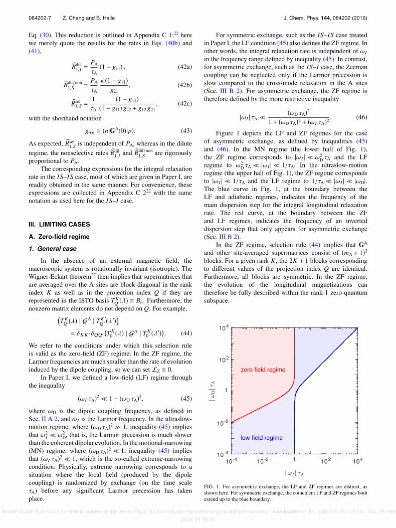
Figure 1 depicts the LF and ZF regimes for the caseof asymmetric exchange, as defined by inequalities (45)and (46). In the MN regime (the lower half of Fig. 1),the ZF regime corresponds to |ωI | ≪ ω2

D τA and the LFregime to ω2

D τA ≪ |ωI | ≪ 1/τA. In the ultraslow-motionregime (the upper half of Fig. 1), the ZF regime correspondsto |ωI | ≪ 1/τA and the LF regime to 1/τA ≪ |ωI | ≪ |ωD|.The blue curve in Fig. 1, at the boundary between theLF and adiabatic regimes, indicates the frequency of themain dispersion step for the integral longitudinal relaxationrate. The red curve, at the boundary between the ZFand LF regimes, indicates the frequency of an inverteddispersion step that only appears for asymmetric exchange(Sec. III B 2).

In the ZF regime, selection rule (44) implies that GA

and other site-averaged supermatrices consist of (mA + 1)2blocks. For a given rank K , the 2K + 1 blocks correspondingto different values of the projection index Q are identical.Furthermore, all blocks are symmetric. In the ZF regime,the evolution of the longitudinal magnetizations cantherefore be fully described within the rank-1 zero-quantumsubspace.

FIG. 1. For asymmetric exchange, the LF and ZF regimes are distinct, asshown here. For symmetric exchange, the coincident LF and ZF regimes bothextend up to the blue boundary.


2016 19:26:38


2. Two-spin case

For two-spin (IS) systems in the ZF regime, selection rule(44) implies that GA has one diagonal element correspondingto the rank-0 singlet operator T0

0 (11), three identical 3 × 3rank-1 blocks spanned by the operators T1

0 (kIkS), T11 (kIkS),

and T1−1(kIkS), respectively, with (kIkS) = (10), (01) or (11),

and five identical rank-2 diagonal elements corresponding toT2Q(11). Since the matrix is symmetric, there are only 9 unique

elements. The evolution of the longitudinal magnetizations instate A is fully described by the T1

0 (kIkS) block, spanned bythe basis operators (Table S1)22

B1 ≡ T10 (10) = Iz, (47a)

B2 ≡ T10 (01) = Sz, (47b)

B4 ≡ T10 (11) = 1

√2(I− S+ − I+ S−)

= i√

2Ix Sy − Iy Sx

. (47c)

Since longitudinal relaxation in the ZF regime can befully described within the rank-1 zero-quantum subspace,many results can be obtained in analytical form. For example,in Appendix D,22 we derive, for the IS–I case, closed-formexpressions for σA

1 (s), σA2 (s), and σA

4 (s), from which thetime evolution of these spin modes can be obtained by aninverse Laplace transformation. In Appendix D,22 we alsoderive expressions for the integral relaxation rate in Eqs. (39)and (40). For example,

Rdil1, I(0) =

23

PAω2

D τA

5 + (ωD τA)2 , (48a)

Rsel1,S(0) =

2ω2D τA

6 + (ωD τA)2 . (48b)

In the MN regime, Eq. (48a) can be written asRdil

1, I(0) = PA RA1 (0), with an intrinsic A-state relaxation rate

RA1 (0) = (2/15)ω2

D τA. This is as expected, because, for theEMOR model, the MN regime is also the fast-exchangeregime. If relaxation in the A-sites were governed by aninternal motion independent of the exchange kinetics, then theLuz-Meiboom equation, R1 = PA/(τA + 1/RA

1 ), should hold inthe dilute + MN regime.31 However, if Eq. (48a) is cast onthis form, we find that RA

1 (0) = (2/3)ω2D τA/[5 + (ωD τA)2/3],

which agrees with the foregoing expression only in the MN(fast-exchange) regime. This inconsistency arises because theLuz-Meiboom equation is not valid for the EMOR model,where the intrinsic relaxation is induced by the exchangeitself so that the MN condition (ωD τA)2 ≪ 1 is automaticallyviolated as soon as we leave the fast-exchange regime.

B. Motional-narrowing regime

1. General case

In the MN regime, where (ωD τA)2 ≪ 1, the compositespin density operator evolves according to the “stochasticRedfield equation” (SRE)

ddt

σ(t) = (W − i L0 − R)σ(t), (49)

where W is same exchange superoperator (8) as in SLE(7) and R is the relaxation superoperator prescribed by the

BWR perturbation theory.7 The Liouvillian L0 is associatedwith the time-independent part of the spin Hamiltonian that isunaffected by the exchange process. For symmetric exchangein general and for asymmetric exchange with only onenonlabile spin (mA = mB + 1), the static Hamiltonian onlycontains the Zeeman coupling so L0 = LZ. For example,this is true for the IS–IS and IS–I cases. However, forasymmetric exchange with mA ≥ mB + 2 (e.g., ISP–I), so theA sites contain at least two nonlabile spins, L0 includes thestatic dipole coupling(s) besides the Zeeman coupling.

Like SLE (7), SRE (49) can be solved in site space, infull analogy with the treatment in Appendix B.22 Specifically,Eqs. (25) and (28) remain valid, but Eq. (30) is replaced by

GA(s) = [s τA 1A +K + i Lα0 τA + RατA]−1 , (50)

where the angular brackets indicate the same isotropicorientational average as in Eq. (30) and Rα is the orientation-dependent relaxation supermatrix for site α. As noted inSec. II D 1, the isotropically averaged supermatrix GA(s) isblock-diagonal in the projection index Q. To determine theintegral longitudinal relaxation rate, as described in Sec. II E,we only need the Q = 0 block of the supermatrix

GA(0) = (Λα)−1 , (51)

with

Λα ≡ K + i Lα0 τA + RατA. (52)

In the EMOR model, exchange plays two roles: ittransfers spin modes between the A and B states and itinduces relaxation by randomizing the orientation of thedipole vector(s) in the A sites. In SLE (7), both of theseroles are played by the exchange superoperator W . In theSRE (49), on the other hand, the first role is played by theexchange superoperator W , which describes the transfer(or decorrelation) of local spin modes σα

n (t), while thesecond role is played by the orientation-dependent relaxationsuperoperator Rα, which describes relaxation induced byorientational randomization of the dipole vector(s) in site α.Because of the dual role played by exchange in the EMORmodel, the MN condition (ωD τA)2 ≪ 1 not only ensures thatthe BWR theory is valid, but it also corresponds to the fast-exchange limit of the SRE because Rα τA ≈ (ωD τA)2 ≪ 1. Toderive the integral relaxation rate in the MN regime from SRE(49), we must therefore implement the MN condition twice:first in obtaining the relaxation supermatrix Rα from the BWRtheory7 and then in implementing the fast-exchange limit byexpanding the matrix inverse (Λα)−1 to first order in ∥Rα∥ τA,that is, to second order in ωD τA.

The theoretical analysis of relaxation in the MN regimeis greatly simplified by making full use of symmetry.32–34

As noted above, rotational symmetry ensures that we onlyneed to consider the Q = 0 block of the isotropically averagedsupermatrix GA(0). In contrast, the relaxation supermatrix Rα

in Eq. (52) pertains to a site α with a particular orientation soit is not block-diagonal in Q. However, in the MN regime, therelaxation problem can be further simplified by exploiting spininversion conjugation (SIC) symmetry.32–34 The ISTOs havedefinite SIC parity (either odd or even) and the superoperatorsi LZ and Rα both have even SIC parity.32–34 According


2016 19:26:38


to the basic orthogonality theorem of group theory,35 thesupermatrices i LZ and Rα in the ISTO basis can then havenonzero elements only between basis operators of the sameparity. If we order the basis operators so that the odd operators(including the single-spin longitudinal operators) precede theeven operators, then the supermatrices i LZ and Rα are block-diagonal. For exchange cases with less than two nonlabilespins, so that Lα

0 = LZ, it then follows (since matrix inversiondoes not alter the block structure and since K is diagonal) thatalso the supermatrixΛα in Eq. (52) is block-diagonal. As longas we are concerned with longitudinal relaxation, we thereforeneed to consider only the odd-parity zero-quantum subblock ofthe GA(0) supermatrix. This partitioning of the Q = 0 subspaceon the basis of SIC parity is helpful also for exchange caseswith two or more nonlabile spins, even though the odd andeven subblocks are then coupled because the superoperatori LD associated with the static dipole coupling(s) has odd SICparity.34

2. Two-spin case

If we reorder the 15 basis operators in Table S122 sothat the six odd-parity (single-spin) operators (including Izand Sz) precede the nine even-parity (two-spin) operators, thesupermatrix Λα in Eq. (52) is block-diagonal. Longitudinalrelaxation is fully described by the odd 6 × 6 block. Orderingthe odd basis operators as Iz, I+, I−, Sz, S+, S−, we can thenpartition Λα into 3 × 3 submatrices as

Λα =

ΛαI I Λα

I S

ΛαSI Λα

SS

, (53)

where, for the IS–I case,

ΛαI I = 1 + τA(Rα

I I + i ωI Q), (54a)Λα

I S = τA RαI S, (54b)

ΛαSI = τA Rα

SI , (54c)

ΛαSS = τA(Rα

SS + i ωS Q). (54d)

Here, 1 is the 3 × 3 identity matrix and Q is a diagonalmatrix with diagonal elements [0, 1, −1]. To obtain Eq. (54),we also noted that, according to Eq. (17), KI I = 1 andKI S = KSI = KSS = 0.

For the elements of the four relaxation submatrices,given explicitly in Appendix E,22 we use a notation where,e.g., RI S

z+ = (T10 (10) |Rα

I S |T11 (01)) = −2−1/2 (Iz |Rα

I S | S+). Theselocal (orientation-dependent) relaxation rates are of four kinds.First, there are longitudinal (RI I

zz and RSSzz ) and transverse

(RI I±± and RSS

±±) auto-spin auto-mode rates. Second, there arelongitudinal (RI S

zz and RSIzz ) and transverse (RI S

±± and RSI±±)

cross-spin auto-mode rates. Auto-spin and cross-spin ratesalso occur in the two-spin Solomon equations,7 but they arethen isotropically averaged. Third, there are the auto-spincross-mode rates RI I

z±, RI I±z, and RI I

±∓, and the correspondingrates for spin S. Finally, there are cross-spin cross-mode rates,like RI S

z±. All these rates pertain to a particular site α and theytherefore depend on the orientation of the dipole vector in thatsite as detailed in Appendix E.22

The cross-mode rates couple the longitudinal andtransverse magnetizations of the same or different spins. This

coupling is a consequence of the spatial anisotropy of the Asites. Indeed, we show in Appendix E22 that all cross-moderates vanish after isotropic averaging. As shown below, suchaveraging occurs in the symmetric IS–IS case, where thesame I–S pair exchanges rapidly among the A sites (viathe B site), but not in the asymmetric IS–I case, where thetwo spins are no longer correlated after the exchange. Asshown explicitly in Appendix E,22 the cross-mode rates areonly effective in the ZF regime, as defined by Eq. (46). Athigher fields, they become nonsecular, that is, the longitudinaland transverse magnetizations are decoupled by the Larmorprecession, which then is much faster than the (local) cross-mode relaxation.

All the local relaxation rates, except for the longitudinalauto-mode rates RI I

zz , RSSzz , and RI S

zz = RSIzz , involve both the

even (real) and the odd (imaginary) parts of the complexspectral density function (Appendix E22). However, the oddspectral density function (OSDF) has no effect on longitudinalrelaxation in the two-spin cases. In the IS–IS case, isotropicaveraging cancels the cross-mode rates so only the longitudinalauto-mode rates are relevant. In the IS–I case, the cross-moderates are only effective in the ZF regime, where the OSDF isnegligibly small compared to the real part. So, in either case,the OSDF only affects the evolution of the transverse spinmodes, giving rise to the well-known second-order dynamicfrequency shift.36 However, for larger spin systems, the OSDFcan also affect the longitudinal modes, e.g., in the ISP–ISPcase.34

Returning now to the derivation of the integral relaxationrate for the IS–I case, we invert the partitioned matrix inEq. (53), obtaining for the I I block

[(Λα)−1]I I = Λα

I I − ΛαI S (Λα

SS)−1ΛαSI

−1

=Z + τA(Rα

I I − ΓαI I)

−1, (55)

where Eq. (54) was used in the second step. Here we havealso defined the diagonal matrix

Z ≡ 1 + i ωI τA Q, (56)

and the “cross relaxation” matrix

ΓαI I ≡ Rα

I S

Rα

SS + i ωS Q−1Rα

SI . (57)

We now expand the inverse in Eq. (55) to second order inωD τA and perform the isotropic site average, to obtain

[(Λα)−1]I I = Z−1 − τA Z−1 RαI I

−ΓαI I

Z−1. (58)

We are primarily interested in the I-spin integralrelaxation rate in the dilute regime. This rate only involves thematrix element

g11 = (1 |GA(0)| 1) = (1 | [(Λα)−1]I I | 1). (59)

Combination of Eqs. (42a) and (56)–(59) yields

Rdil1, I = PA

RI Izz

−ΓI Izz

, (60)

where RI Izz ≡ (1 |Rα

I I | 1) and ΓI Izz ≡ (1 |ΓαI I | 1). The first term

within square brackets in Eq. (60) is the well-known7,21

longitudinal auto-spin relaxation rate, averaged over theisotropic distribution of A sites (Appendix E22),


2016 19:26:38


RI Izz

=

245

ω2D [ j(ωI − ωS) + 3 j(ωI) + 6 j(ωI + ωS) ] ,

(61)

with the reduced spectral density function given by

j(ω) = τA

1 + (ω τA)2 . (62)

The second term in Eq. (60) accounts for cross-spin aswell as cross-mode relaxation. Cross-mode relaxation onlycomes into play in the ZF regime, where all relaxationchannels are secular, meaning that all oscillating factors inEq. (E.28)22 can be replaced by unity. According to Eq. (57),the cross relaxation matrix element ΓI Izz = (1 |ΓαI I | 1) only hascontributions from the first row of Rα

I S and from the firstcolumn of Rα

SI . The four off-diagonal elements in this groupof six elements involve the cross-spin cross-mode rates RI S

z±and RSI

±z , all of which are multiplied by oscillating factorsexp(± i ωS t) in Eq. (E.28).22 Two conclusions follow. First,the longitudinal-transverse cross-mode relaxation contributionto Rdil

1, I in the zero-field regime involves the four cross-spin cross-mode rates RI S

z± and RSI±z and the four auto-spin-S

cross-mode rates RSSz± and RSS

±z , but it does not involve thefour auto-spin-I cross-mode rates RI I

z± and RI I±z. Second, for

a heteronuclear spin pair, with ωS , ωI , the entire cross-mode contribution to Rdil

1, I disappears when |ωS | ≫ ω2D τA

(Sec. IV B).Outside the ZF regime, cross-mode relaxation is

nonsecular and can therefore be neglected. The four relaxationsubmatrices are then diagonal so Eqs. (57) and (60) yield

Rdil1, I = PA

RI Izz

−

(RI Szz )2

RSSzz

, (63)

where the orientation-dependent auto-spin and cross-spin ratesin the second term are given in Appendix E.22 In the LF +MNregime, which is also the extreme-narrowing regime (Sec.III A 1), these rates are given by Eqs. (E.35a) and (E.35b).22

Substitution into Eq. (63) yields after isotropic averaging

Rdil1, I = c PAω

2D τA, (64)

with the numerical constant

c ≡ 1

0dx

(1 − x2)(1 + 3 x2)(5 − 3 x2) = 0.267 779. . .. (65)

Result (63) is not valid in the ZF regime, where there iscross-mode coupling. In the ZF + MN regime, Eq. (48a)reduces to

Rdil1, I(0) =

215

PAω2D τA, (66)

which is a factor 2.008 343 . . . smaller than the result inEq. (64). It is clear, therefore, that longitudinal-transversecross-mode coupling slows down the longitudinal relaxationof the labile I-spin. As the Larmor frequency increases frombelow ω2

D τA to above this value, the integral relaxation rateRdil

1, I thus exhibits an inverted dispersion step. The locus ofthis dispersion step is indicated by the red curve in Fig. 1 (theboundary between the ZF and LF regimes).

It is instructive to contrast these results for the asymmetricIS–I case with the corresponding results for the symmetric

IS–IS case.20 For the symmetric case, Eq. (41a) is replacedby (Appendix C 222)

Rdil/non1, I =

UBB

11 + κUBB12

−1, (67a)

Rdil/non1, I S = (1 + κ)UBB

11 +UBB21 + κ (UBB

12 +UBB22 )−1

, (67b)

depending on whether we observe spin I only or both spins.Spin Liouville space is now spanned by the same 15 basisoperators (Table S1)22 for both states A and B. Further-more, T = K = 1 and Eqs. (28a) and (50) yield (in the diluteregime)

UBB(0) = τA

PA[1 + i LZ τB −GA(0)]−1 (68)

and

GA(0) =[1 + i LZ τA + Rα τA]−1

= [1 + i LZ τA]−1 − [1 + i LZ τA]−1 τA ⟨Rα⟩ [1 + i LZ τA]−1,

(69)

where we have invoked the MN approximation by expandingGA(0) to second order in ωD τA. In contrast to the asymmetricexchange case, relaxation now enters only via the isotropicallyaveraged relaxation supermatrix ⟨Rα⟩. This has two importantconsequences. First, all cross-mode relaxation rates vanish(Appendix E22). Second, because the relaxation supermatrixis now isotropically averaged, we can invoke the Wigner-Eckart theorem to establish that ⟨Rα⟩ is block-diagonal in Q.To describe longitudinal relaxation, we therefore only needto consider the 5 × 5 Q = 0 block. Moreover, because Rα isinvariant under SIC, this block decomposes into an odd-parity2 × 2 block (spanned by Iz and Sz) and an even-parity 3 × 3block (spanned by the basis operators B3, B4, and B5 in TableS1).22 Although the Q = 0 block of LZ is not diagonal forωI , ωS, we only need the odd-parity sub-block, which is the2 × 2 null matrix. We thus obtain from Eqs. (68) and (69),

UBB(0) = ⟨Rα⟩−1

PA=

1PA

ρI σ

σ ρS

−1

, (70)

where the familiar expressions for the longitudinal auto-spin rates ρI ≡

RI Izz

and ρS ≡

RSSzz

and cross-spin rate

σ ≡RI Szz

=RSIzz

are given in Eq. (E.32) of Appendix E.22

Combination of Eqs. (67) and (70) then yields

Rdil/non1, I = PA

(ρI ρS − σ2)(ρS − κ σ) , (71a)

Rdil/non1, I S = PA

(1 + κ)(ρI ρS − σ2)(ρS − σ) + κ (ρI − σ) , (71b)

in agreement with the results (using a slightly differentnotation) of Paper I. In particular, for symmetric exchangeof a pair of homonuclear (κ = γS/γI = 1) and isochronous(ωI = ωS) spins, both rates in Eq. (71) reduce to the familiarform

Rdil/non1, I = Rdil/non

1, I S = PA (ρ + σ)=

215

PAω2D [ j(ωI) + 4 j(2ωI) ] . (72)

In the MN regime, rotational and SIC symmetries ensurethat longitudinal relaxation can be fully described within


2016 19:26:38


the two-dimensional zero-quantum odd-parity subspacecorresponding to the longitudinal spin modes Iz and Sz. Thisis true for symmetric as well as for asymmetric exchange.The crucial difference between these exchange cases in theMN regime is that the intrinsic relaxation rates in the Asites are isotropically averaged only for the symmetric IS–IScase. For the asymmetric IS–I case, the orientation-dependentrelaxation in the A sites must, in general, be described in thesix-dimensional odd-parity subspace corresponding to thesingle-spin longitudinal and transverse local modes. However,outside the ZF regime, the longitudinal local spin modes Iαzand Sα

z are decoupled from the transverse local spin modes Iα±and Sα

± .

IV. NUMERICAL RESULTS FOR TWO-SPIN SYSTEMS

In this section, we illustrate the theoretical results ob-tained in Secs. II and III by numerical calculations. Except inSec. IV B, we consider a homonuclear and effectively isochro-nous (ωS = ωI) spin pair. The dipole coupling frequencyis set to ωD = 1 × 105 rad s−1, corresponding to an internuclearseparation of r I S = 2.245 Å for two protons, and the fractionbound I spins is PA = 10−3, corresponding to the diluteregime. Following the standard convention, we take ωI to bepositive. We focus on the asymmetric IS–I case, highlightingdifferences compared to the symmetric IS–IS case.

A. Cross-mode relaxation

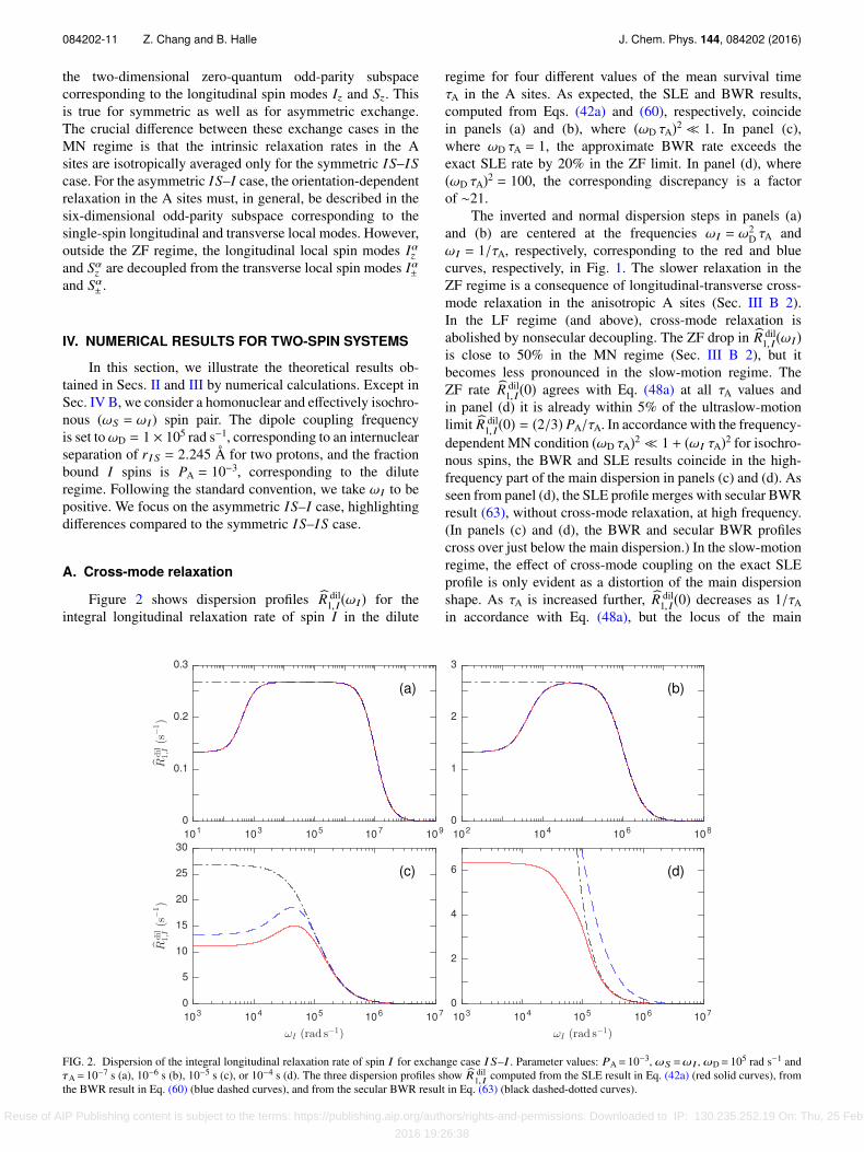
Figure 2 shows dispersion profiles R dil1, I(ωI) for the

integral longitudinal relaxation rate of spin I in the dilute

regime for four different values of the mean survival timeτA in the A sites. As expected, the SLE and BWR results,computed from Eqs. (42a) and (60), respectively, coincidein panels (a) and (b), where (ωD τA)2 ≪ 1. In panel (c),where ωD τA = 1, the approximate BWR rate exceeds theexact SLE rate by 20% in the ZF limit. In panel (d), where(ωD τA)2 = 100, the corresponding discrepancy is a factorof ∼21.

The inverted and normal dispersion steps in panels (a)and (b) are centered at the frequencies ωI = ω2

D τA andωI = 1/τA, respectively, corresponding to the red and bluecurves, respectively, in Fig. 1. The slower relaxation in theZF regime is a consequence of longitudinal-transverse cross-mode relaxation in the anisotropic A sites (Sec. III B 2).In the LF regime (and above), cross-mode relaxation isabolished by nonsecular decoupling. The ZF drop in R dil

1, I(ωI)is close to 50% in the MN regime (Sec. III B 2), but itbecomes less pronounced in the slow-motion regime. TheZF rate R dil

1, I(0) agrees with Eq. (48a) at all τA values andin panel (d) it is already within 5% of the ultraslow-motionlimit R dil

1, I(0) = (2/3) PA/τA. In accordance with the frequency-dependent MN condition (ωD τA)2 ≪ 1 + (ωI τA)2 for isochro-nous spins, the BWR and SLE results coincide in the high-frequency part of the main dispersion in panels (c) and (d). Asseen from panel (d), the SLE profile merges with secular BWRresult (63), without cross-mode relaxation, at high frequency.(In panels (c) and (d), the BWR and secular BWR profilescross over just below the main dispersion.) In the slow-motionregime, the effect of cross-mode coupling on the exact SLEprofile is only evident as a distortion of the main dispersionshape. As τA is increased further, R dil

1, I(0) decreases as 1/τAin accordance with Eq. (48a), but the locus of the main

FIG. 2. Dispersion of the integral longitudinal relaxation rate of spin I for exchange case I S–I . Parameter values: PA= 10−3, ωS =ωI , ωD= 105 rad s−1 andτA= 10−7 s (a), 10−6 s (b), 10−5 s (c), or 10−4 s (d). The three dispersion profiles show R dil

1, I computed from the SLE result in Eq. (42a) (red solid curves), fromthe BWR result in Eq. (60) (blue dashed curves), and from the secular BWR result in Eq. (63) (black dashed-dotted curves).


2016 19:26:38


dispersion remains at ωI ≈ ωD, as demonstrated in Paper I forthe symmetric IS–IS case.

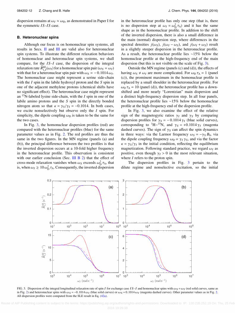
B. Heteronuclear spins

Although our focus is on homonuclear spin systems, allresults in Secs. II and III are valid also for heteronuclearspin systems. To illustrate the different relaxation behaviorsof homonuclear and heteronuclear spin systems, we shallcompare, for the IS–I case, the dispersion of the integralrelaxation rate Rdil

1, I(ωI) for a homonuclear spin pair (ωS = ωI)with that for a heteronuclear spin pair with ωS = − 0.1014ωI .The homonuclear case might represent a serine side-chainwith the I spin in the labile hydroxyl proton and the S spin inone of the adjacent methylene protons (chemical shifts haveno significant effect). The heteronuclear case might representan 15N-labeled lysine side-chain, with the I spin in one of thelabile amino protons and the S spin in the directly bondednitrogen atom so that κ = γS/γI = −0.1014. In both cases,we excite nonselectively but observe only the I spin. Forsimplicity, the dipole coupling ωD is taken to be the same forthe two cases.

In Fig. 3, the homonuclear dispersion profiles (red) arecompared with the heteronuclear profiles (blue) for the sameparameter values as in Fig. 2. The red profiles are thus thesame in the two figures. In the MN regime (panels (a) and(b)), the principal difference between the two profiles is thatthe inverted dispersion occurs at a 10-fold higher frequencyin the heteronuclear profile. This observation is consistentwith our earlier conclusion (Sec. III B 2) that the effect ofcross-mode relaxation vanishes when ωS exceeds ω2

D τA, thatis, when ωI & 10ω2

D τA. Consequently, the inverted dispersion

in the heteronuclear profile has only one step (that is, thereis no dispersion step at ωI ≈ ω2

D τA) and it has the sameshape as in the homonuclear profile. In addition to the shiftof the inverted dispersion, there is also a small difference inthe main (normal) dispersion step, where differences in thespectral densities j(ωS), j(ωI − ωS), and j(ωI + ωS) resultin a slightly steeper dispersion in the heteronuclear profile.As a result, the heteronuclear profile lies ∼15% below thehomonuclear profile at the high-frequency end of the maindispersion (but this is not visible on the scale of Fig. 3).

Outside the MN regime (panels (c) and (d)), the effects ofhaving ωS , ωI are more complicated. For ωD τA = 1 (panel(c)), the prominent maximum in the homonuclear profile isreplaced by a small shoulder in the heteronuclear profile. ForωD τA = 10 (panel (d)), the heteronuclear profile has a down-shifted and more nearly “Lorentzian” main dispersion anda distinct high-frequency dispersion step. In all four panels,the heteronuclear profile lies ∼15% below the homonuclearprofile at the high-frequency end of the dispersion profile.

In Fig. 3, we also examine the effect of the relativesign of the magnetogyric ratios γI and γS by comparingdispersion profiles for γS = − 0.1014 γI (blue solid curves),corresponding to 1H−15N, and γS = +0.1014 γI (magentadashed curves). The sign of γS can affect the spin dynamicsin three ways: via the Larmor frequency ωS = −γS B0, viathe dipole coupling frequency ωD ∝ γI γS, and via the factorκ = γS/γI in the initial condition, reflecting the equilibriummagnetization. Following standard practice, we regard ωI aspositive, even though γI > 0 in the most relevant situation,where I refers to the proton spin.

The dispersion profiles in Fig. 3 pertain to thedilute regime and nonselective excitation, so the initial

FIG. 3. Dispersion of the integral longitudinal relaxation rate of spin I for exchange case I S–I and homonuclear spins with ωS =ωI (red solid curves, same asin Fig. 2) and heteronuclear spins with ωS =−0.1014ωI (blue solid curves) or ωS = 0.1014ωI (magenta dashed curves). Other parameter values as in Fig. 2.All dispersion profiles were computed from the SLE result in Eq. (42a).


2016 19:26:38


I-spin magnetization is strongly dominated by the equi-librium magnetization in state B. Consequently (thesign of) κ has no significant effect on the dispersionprofiles.

In the MN regime (panels (a) and (b)), the spin dynamicsonly depend on the square of ωD so the only effect of reversingsign of γS is to interchange the spectral densities j(ωI − ωS)and j(ωI + ωS).37 As seen from panels (a) and (b), thiseffect is rather small; the maximum effect (barely visible inFig. 3) occurs in the adiabatic regime (ωI τA ≫ 1), whereRdil

1, I(ωI) is ∼14% smaller for γS = +0.1014 γI than for γS= −0.1014 γI .

Outside the MN regime (panels (c) and (d)), a signreversal in γS makes the dispersion profile more smooth,without any pronounced shoulder. As in the MN regime,this effect is entirely due to the sign reversal of ωS.Although the evolution of some spin modes dependson the sign of ωD (for example, see Eqs. (D.9f) and(D.18)22), the evolution of the longitudinal magnetizationsonly involves even powers of ωD. As in the MN regime,Rdil

1, I(ωI) is ∼14% smaller for γS = + 0.1014 γI than forγS = − 0.1014 γI at the high-frequency end of the dispersionprofile.

C. Symmetric versus asymmetric exchange

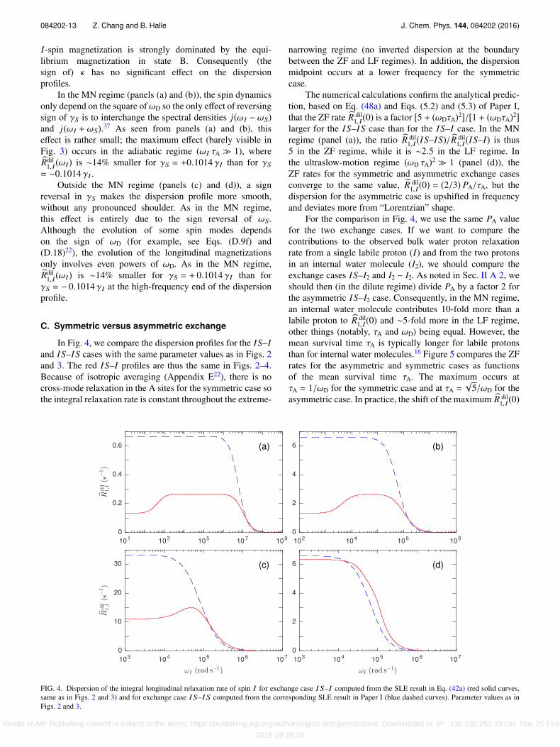
In Fig. 4, we compare the dispersion profiles for the IS–Iand IS–IS cases with the same parameter values as in Figs. 2and 3. The red IS–I profiles are thus the same in Figs. 2–4.Because of isotropic averaging (Appendix E22), there is nocross-mode relaxation in the A sites for the symmetric case sothe integral relaxation rate is constant throughout the extreme-

narrowing regime (no inverted dispersion at the boundarybetween the ZF and LF regimes). In addition, the dispersionmidpoint occurs at a lower frequency for the symmetriccase.

The numerical calculations confirm the analytical predic-tion, based on Eq. (48a) and Eqs. (5.2) and (5.3) of Paper I,that the ZF rate R dil

1, I(0) is a factor [5 + (ωDτA)2]/[1 + (ωDτA)2]larger for the IS–IS case than for the IS–I case. In the MNregime (panel (a)), the ratio R dil

1, I(IS–IS)/R dil1, I(IS–I) is thus

5 in the ZF regime, while it is ∼2.5 in the LF regime. Inthe ultraslow-motion regime (ωD τA)2 ≫ 1 (panel (d)), theZF rates for the symmetric and asymmetric exchange casesconverge to the same value, R dil

1, I(0) = (2/3) PA/τA, but thedispersion for the asymmetric case is upshifted in frequencyand deviates more from “Lorentzian” shape.

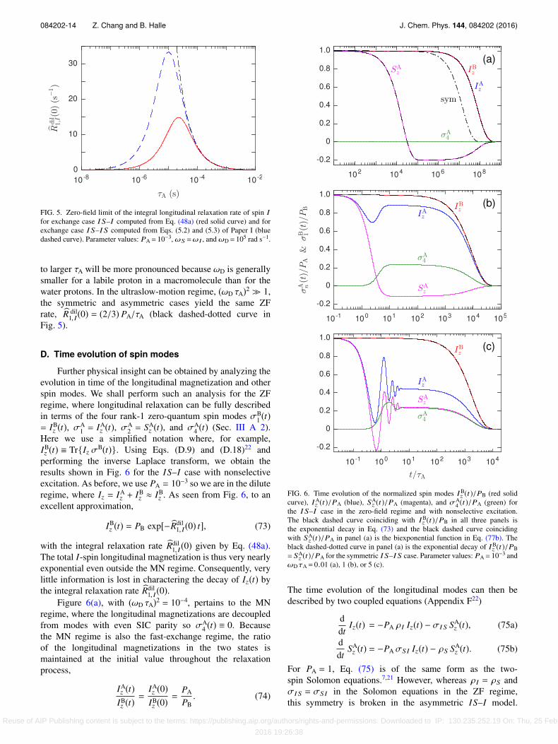
For the comparison in Fig. 4, we use the same PA valuefor the two exchange cases. If we want to compare thecontributions to the observed bulk water proton relaxationrate from a single labile proton (I) and from the two protonsin an internal water molecule (I2), we should compare theexchange cases IS–I2 and I2 − I2. As noted in Sec. II A 2, weshould then (in the dilute regime) divide PA by a factor 2 forthe asymmetric IS–I2 case. Consequently, in the MN regime,an internal water molecule contributes 10-fold more than alabile proton to R dil

1, I(0) and ∼5-fold more in the LF regime,other things (notably, τA and ωD) being equal. However, themean survival time τA is typically longer for labile protonsthan for internal water molecules.16 Figure 5 compares the ZFrates for the asymmetric and symmetric cases as functionsof the mean survival time τA. The maximum occurs atτA = 1/ωD for the symmetric case and at τA =

√5/ωD for the

asymmetric case. In practice, the shift of the maximum R dil1, I(0)

FIG. 4. Dispersion of the integral longitudinal relaxation rate of spin I for exchange case I S–I computed from the SLE result in Eq. (42a) (red solid curves,same as in Figs. 2 and 3) and for exchange case I S–I S computed from the corresponding SLE result in Paper I (blue dashed curves). Parameter values as inFigs. 2 and 3.


2016 19:26:38


FIG. 5. Zero-field limit of the integral longitudinal relaxation rate of spin Ifor exchange case I S–I computed from Eq. (48a) (red solid curve) and forexchange case I S–I S computed from Eqs. (5.2) and (5.3) of Paper I (bluedashed curve). Parameter values: PA= 10−3, ωS =ωI , and ωD= 105 rad s−1.

to larger τA will be more pronounced because ωD is generallysmaller for a labile proton in a macromolecule than for thewater protons. In the ultraslow-motion regime, (ωD τA)2 ≫ 1,the symmetric and asymmetric cases yield the same ZFrate, R dil

1, I(0) = (2/3) PA/τA (black dashed-dotted curve inFig. 5).

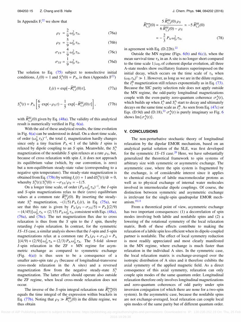
D. Time evolution of spin modes

Further physical insight can be obtained by analyzing theevolution in time of the longitudinal magnetization and otherspin modes. We shall perform such an analysis for the ZFregime, where longitudinal relaxation can be fully describedin terms of the four rank-1 zero-quantum spin modes σB

1 (t)= IB

z (t), σA1 = IA

z (t), σA2 = SA

z (t), and σA4 (t) (Sec. III A 2).

Here we use a simplified notation where, for example,IBz (t) ≡ TrIz σB(t). Using Eqs. (D.9) and (D.18)22 and

performing the inverse Laplace transform, we obtain theresults shown in Fig. 6 for the IS–I case with nonselectiveexcitation. As before, we use PA = 10−3 so we are in the diluteregime, where Iz = IA

z + IBz ≈ IB

z . As seen from Fig. 6, to anexcellent approximation,

IBz (t) = PB exp[−Rdil

1, I(0) t], (73)

with the integral relaxation rate Rdil1, I(0) given by Eq. (48a).

The total I-spin longitudinal magnetization is thus very nearlyexponential even outside the MN regime. Consequently, verylittle information is lost in charactering the decay of Iz(t) bythe integral relaxation rate Rdil

1, I(0).Figure 6(a), with (ωD τA)2 = 10−4, pertains to the MN

regime, where the longitudinal magnetizations are decoupledfrom modes with even SIC parity so σA

4 (t) ≡ 0. Becausethe MN regime is also the fast-exchange regime, the ratioof the longitudinal magnetizations in the two states ismaintained at the initial value throughout the relaxationprocess,

IAz (t)

IBz (t)=

IAz (0)

IBz (0)

=PA

PB. (74)

FIG. 6. Time evolution of the normalized spin modes IBz (t)/PB (red solid

curve), IAz (t)/PA (blue), SA

z (t)/PA (magenta), and σA4 (t)/PA (green) for

the I S–I case in the zero-field regime and with nonselective excitation.The black dashed curve coinciding with IB

z (t)/PB in all three panels isthe exponential decay in Eq. (73) and the black dashed curve coincidingwith SA

z (t)/PA in panel (a) is the biexponential function in Eq. (77b). Theblack dashed-dotted curve in panel (a) is the exponential decay of IB

z (t)/PB= SA

z (t)/PA for the symmetric I S–I S case. Parameter values: PA= 10−3 andωDτA= 0.01 (a), 1 (b), or 5 (c).

The time evolution of the longitudinal modes can then bedescribed by two coupled equations (Appendix F22)

ddt

Iz(t) = −PA ρI Iz(t) − σI S SAz (t), (75a)

ddt

SAz (t) = −PA σSI Iz(t) − ρS SA

z (t). (75b)

For PA = 1, Eq. (75) is of the same form as the two-spin Solomon equations.7,21 However, whereas ρI = ρS andσI S = σSI in the Solomon equations in the ZF regime,this symmetry is broken in the asymmetric IS–I model.


2016 19:26:38


In Appendix F,22 we show that

ρI =29ω2

D τA, (76a)

ρS =59ω2

D τA, (76b)

σI S =49ω2

D τA, (76c)

σSI =19ω2

D τA. (76d)

The solution to Eq. (75) subject to nonselective initialconditions, Iz(0) = 1 and SA

z (0) = PA, is then (Appendix F22)

Iz(t) = exp[−Rdil1, I(0) t], (77a)

SAz (t) = PA

65

exp(−ρS t) − 15

exp[−Rdil1, I(0) t]

, (77b)

with Rdil1, I(0) given by Eq. (48a). The validity of this analytical

result is numerically verified in Fig. 6(a).With the aid of these analytical results, the time evolution

in Fig. 6(a) can be understood in detail. On a short time scale,of order (ω2

D τA)−1, the total Iz magnetization hardly changessince only a tiny fraction PA ≪ 1 of the labile I spins isrelaxed by dipole coupling to an S spin. Meanwhile, the SA

z

magnetization of the nonlabile S spin relaxes at a rate ρS, but,because of cross relaxation with spin I, it does not approachits equilibrium value (which, by our convention, is zero)but a non-equilibrium steady-state value (corresponding to anegative spin temperature). The steady-state magnetization isobtained from Eq. (75b) by setting Iz(t) = 1 and dSA

z (t)/dt = 0,whereby SA

z (t)/SAz (0) = −σSI/ρS = −1/5.

On a longer time scale, of order (PAω2D τA)−1, the I-spin

and S-spin magnetizations relax to their (zero) equilibriumvalues at a common rate Rdil

1, I(0). By inserting the steady-state SA

z magnetization, −(1/5) PA Iz(t), in Eq. (75a), wesee that this rate is given by PA (ρI − σI S/5) = PA [(2/9)− (4/45)]ω2

D τA = (2/15) PAω2D τA, consistent with Eqs. (48a),

(76a), and (76c). The net magnetization flux due to crossrelaxation is thus from the S spin to the I spin, therebyretarding I-spin relaxation. In contrast, for the symmetricIS–IS case, a similar analysis shows that the I-spin and S-spinmagnetizations relax at a common rate PA (ρI + σI S) = PA[(4/9) + (2/9)]ω2

D τA = (2/3) PAω2D τA. The 5-fold slower

I-spin relaxation in the ZF + MN regime for asym-metric exchange as compared to symmetric exchange(Fig. 4(a)) is thus seen to be a consequence of asmaller auto-spin rate ρI (because of longitudinal-transversecross-mode relaxation in the A sites) and a reversedmagnetization flow from the negative steady-state SA

z

magnetization. The latter effect should operate also outsidethe ZF regime, when local cross-mode relaxation does notoccur.

The inverse of the S-spin integral relaxation rate Rnon1,S(0)

equals the time integral of the expression within brackets inEq. (77b). Noting that ρS ≫ Rdil

1, I(0) in the dilute regime, wethus obtain

Rnon1,S(0) =

5 Rdil1, I(0) ρS

6 Rdil1, I(0) − ρS

≈ −5 Rdil1, I(0)

= − 23

PAω2D τA, (78)

in agreement with Eq. (D.22b).22

Outside the MN regime (Figs. 6(b) and 6(c)), when themean survival time τA in an A site is no longer short comparedto the time scale 1/ωD of coherent dipolar evolution, all threeA-state modes show oscillatory features superimposed on theinitial decay, which occurs on the time scale of τA when(ωD τA)2 ≫ 1. However, as long as we are in the dilute regime,the IB

z magnetization still relaxes exponentially as in Eq. (73).Because the SIC parity selection rule does not apply outsidethe MN regime, the odd-parity longitudinal magnetizationscouple with the even-parity zero-quantum coherence σA

4 (t),which builds up when IA

z and SAz start to decay and ultimately

decays on the same time scale as IBz . As seen from Eq. (47c) or

Eqs. (D.9d) and (D.18),22 σA4 (t) is purely imaginary so Fig. 6

shows ImσA4 (t).

V. CONCLUSIONS

The non-perturbative stochastic theory of longitudinalrelaxation by the dipolar EMOR mechanism, based on ananalytical partial solution of the SLE, was first developedfor the symmetric IS–IS case.20 Here, we have substantiallygeneralized the theoretical framework to spin systems ofarbitrary size with symmetric or asymmetric exchange. Theasymmetric case, where the spin system is fragmented bythe exchange, is of considerable interest since it appliesto chemical exchange of labile macromolecular protons aswell as to physical exchange of internal water moleculesinvolved in intermolecular dipole couplings. Of course, thedistinction between symmetric and asymmetric exchangeis irrelevant for the single-spin quadrupolar EMOR mech-anism.10,11

From a theoretical point of view, asymmetric exchangehas two important consequences: (1) a decorrelation of spinmodes involving both labile and nonlabile spins and (2) alowering of the rotational symmetry of the local relaxationmatrix. Both of these effects contribute to making therelaxation of a labile spin less efficient when its dipole-coupledpartner is nonlabile. The effect of local symmetry reductionis most readily appreciated and most clearly manifestedin the MN regime, where exchange is much faster thanrelaxation in the individual A sites. In the symmetric case,the local relaxation matrix is exchange-averaged over theisotropic distribution of A sites and it therefore exhibits theaxial symmetry of the applied magnetic field. As a directconsequence of this axial symmetry, relaxation can onlycouple spin modes of the same quantum order. Longitudinalrelaxation therefore only involves longitudinal magnetizationsand zero-quantum coherences of odd parity under spininversion conjugation (of which there are none for a two-spinsystem). In the asymmetric case, because the nonlabile spinsare not exchange-averaged, local relaxation can couple localspin modes of the same parity but of different quantum order.


2016 19:26:38


In particular, the observed longitudinal relaxation is affectedby local longitudinal-transverse cross-mode relaxation in theA sites. To the best of our knowledge, such cross-moderelaxation phenomena have not previously been described inthe literature.

As an illustration of the general dipolar EMOR theoryand, in particular, of the previously unrecognized20 effectsof asymmetric exchange, we presented here a detailedanalysis of the asymmetric two-spin case IS–I. A varietyof analytical results were obtained for the ZF and MN regimesand numerical results were presented under more generalconditions, including the case of a heteronuclear spin pair. Wedemonstrated how local longitudinal-transverse cross-moderelaxation slows down the observed relaxation of the labile Ispin in the ZF regime and that an unusual inverted dispersionstep occurs at higher fields, where the cross-mode relaxationchannel becomes nonsecular. This inverted dispersion splitsthe extreme-narrowing regime into two sub-regimes, referredto here as the zero-field and low-field regimes. We alsopresented a detailed analysis of the time evolution of the spinmodes in the ZF regime.

The general theoretical framework developed herewill enable a quantitative analysis of frequency-dependentwater-proton longitudinal relaxation in model systems withimmobilized macromolecules and, ultimately, will providea rigorous link between relaxation-based magnetic resonanceimage contrast and the molecular-level properties of the tissue.In a forthcoming report, we apply this framework to a three-spin system ISP, analyzing in detail the ISP–I, ISP–IS, andISP–ISP exchange cases.

ACKNOWLEDGMENTS

This work was financially supported by the SwedishResearch Council.

1S. H. Koenig and R. D. Brown, Prog. Nucl. Magn. Reson. Spectrosc. 22, 487(1990).

2S. H. Koenig and R. D. Brown, Magn. Reson. Med. 30, 685 (1993).3J. P. Korb and R. G. Bryant, J. Chem. Phys. 115, 10964 (2001).

4B. Halle, Magn. Reson. Med. 56, 60 (2006).5E. P. Sunde and B. Halle, J. Am. Chem. Soc. 131, 18214 (2009).6F. V. Chávez and B. Halle, Magn. Reson. Med. 56, 73 (2006).7A. Abragam, The Principles of Nuclear Magnetism (Clarendon Press, Ox-ford, 1961).

8R. Kubo, J. Math. Phys. 4, 174 (1963).9R. Kubo, in Advances in Chemical Physics, edited by K. E. Shuler (Wiley,New York, 1969), Vol. 15, p. 101.

10B. Halle, Prog. Nucl. Magn. Reson. Spectrosc. 28, 137 (1996).11T. Nilsson and B. Halle, J. Chem. Phys. 137, 054503 (2012).12P. Roose, H. Bauwin, and B. Halle, J. Phys. Chem. B 103, 5167 (1999).13F. V. Chávez, E. Persson, and B. Halle, J. Am. Chem. Soc. 128, 4902

(2006).14F. V. Chávez, E. Hellstrand, and B. Halle, J. Phys. Chem. B 110, 21551

(2006).15B. Halle and V. P. Denisov, Biophys. J. 69, 242 (1995).16E. Persson and B. Halle, J. Am. Chem. Soc. 130, 1774 (2008).17S. Kaieda and B. Halle, J. Phys. Chem. B 117, 14676 (2013).18S. Kaieda and B. Halle, J. Phys. Chem. B 119, 7957 (2015).19E. Persson and B. Halle, Proc. Natl. Acad. Sci. U. S. A. 105, 6266

(2008).20Z. Chang and B. Halle, J. Chem. Phys. 139, 144203 (2013).21I. Solomon, Phys. Rev. 99, 559 (1955).22See supplementary material at http://dx.doi.org/10.1063/1.4942026 for

lists of ISTO basis operators (Appendix A); partial solution of the SLE(Appendix B); expressions for integral relaxation rates (Appendix C);analytical results for the ZF (Appendix D) and MN (Appendix E) regimes;and time evolution of Iz and Sz (Appendix F).

23F. Persson and B. Halle, J. Am. Chem. Soc. 135, 8735 (2013).24G. Binsch, J. Am. Chem. Soc. 91, 1304 (1969).25R. R. Ernst, G. Bodenhausen, and A. Wokaun, Principles of Nuclear Mag-

netic Resonance in One and Two Dimensions (Clarendon Press, Oxford,1987).

26N. R. Skrynnikov, T. N. Khazanovich, and B. C. Sanctuary, Mol. Phys. 91,977 (1997).

27D. M. Brink and G. R. Satchler, Angular Momentum, 3rd ed. (ClarendonPress, Oxford, 1994).

28N. R. Skrynnikov and R. R. Ernst, J. Magn. Reson. 137, 276 (1999).29N. G. van Kampen, Stochastic Processes in Physics and Chemistry, 3rd ed.

(North-Holland, Amsterdam, 2007).30F. Persson and B. Halle, J. Chem. Theory Comp. 9, 2838 (2013).31Z. Luz and S. Meiboom, J. Chem. Phys. 40, 2686 (1964).32N. C. Pyper, Mol. Phys. 21, 1 (1971).33S. Szymanski, A. M. Gryff-Keller, and G. Binsch, J. Magn. Reson. 68, 399

(1986).34Z. Chang and B. Halle, J. Chem. Phys. 143, 234201 (2015).35M. Tinkham, Group Theory and Quantum Mechanics (McGraw-Hill, New

York, 1964).36L. G. Werbelow, Encyclopedia of NMR (Wiley, New York, 1996), p. 1776.37L. G. Werbelow, J. Chem. Soc., Faraday Trans. 2 83, 897 (1987).


2016 19:26:38

http://dx.doi.org/10.1016/0079-6565(90)80008-6

http://dx.doi.org/10.1002/mrm.1910300606

http://dx.doi.org/10.1063/1.1417509


http://dx.doi.org/10.1021/ja908144y


http://dx.doi.org/10.1063/1.1703941

http://dx.doi.org/10.1002/9780470143605.ch6

http://dx.doi.org/10.1016/0079-6565(96)90000-X

http://dx.doi.org/10.1063/1.4739297

http://dx.doi.org/10.1021/jp984277l

http://dx.doi.org/10.1021/ja058837n

http://dx.doi.org/10.1021/jp057567s

http://dx.doi.org/10.1016/S0006-3495(95)79895-2

http://dx.doi.org/10.1021/ja0775873

http://dx.doi.org/10.1021/jp409234g

http://dx.doi.org/10.1021/acs.jpcb.5b03214

http://dx.doi.org/10.1073/pnas.0709585105

http://dx.doi.org/10.1063/1.4824105

http://dx.doi.org/10.1103/PhysRev.99.559

http://dx.doi.org/10.1063/1.4942026

http://dx.doi.org/10.1063/1.4942026

http://dx.doi.org/10.1063/1.4942026

http://dx.doi.org/10.1063/1.4942026

http://dx.doi.org/10.1063/1.4942026

http://dx.doi.org/10.1063/1.4942026

http://dx.doi.org/10.1063/1.4942026

http://dx.doi.org/10.1063/1.4942026

http://dx.doi.org/10.1063/1.4942026

http://dx.doi.org/10.1063/1.4942026

http://dx.doi.org/10.1063/1.4942026

http://dx.doi.org/10.1063/1.4942026

http://dx.doi.org/10.1063/1.4942026

http://dx.doi.org/10.1063/1.4942026

http://dx.doi.org/10.1063/1.4942026

http://dx.doi.org/10.1063/1.4942026

http://dx.doi.org/10.1063/1.4942026

http://dx.doi.org/10.1063/1.4942026

http://dx.doi.org/10.1063/1.4942026

http://dx.doi.org/10.1063/1.4942026

http://dx.doi.org/10.1063/1.4942026

http://dx.doi.org/10.1063/1.4942026

http://dx.doi.org/10.1063/1.4942026

http://dx.doi.org/10.1063/1.4942026

http://dx.doi.org/10.1063/1.4942026

http://dx.doi.org/10.1063/1.4942026

http://dx.doi.org/10.1063/1.4942026

http://dx.doi.org/10.1063/1.4942026

http://dx.doi.org/10.1063/1.4942026

http://dx.doi.org/10.1063/1.4942026

http://dx.doi.org/10.1063/1.4942026

http://dx.doi.org/10.1063/1.4942026

http://dx.doi.org/10.1063/1.4942026

http://dx.doi.org/10.1063/1.4942026

http://dx.doi.org/10.1063/1.4942026

http://dx.doi.org/10.1021/ja403405d

http://dx.doi.org/10.1021/ja01034a007

http://dx.doi.org/10.1080/002689797170743

http://dx.doi.org/10.1006/jmre.1998.1666

http://dx.doi.org/10.1021/ct400161u

http://dx.doi.org/10.1063/1.1725581

http://dx.doi.org/10.1080/00268977100101151

http://dx.doi.org/10.1016/0022-2364(86)90334-3

http://dx.doi.org/10.1063/1.4937377

http://dx.doi.org/10.1039/f29878300897

Supplemental Material

Nuclear magnetic relaxation by the dipolar EMOR mechanism:

General theory with applications to two-spin systems

Zhiwei Chang and Bertil Halle

Division of Biophysical Chemistry, Department of Chemistry, Lund University,

POB 124, SE-22100 Lund, Sweden

S1

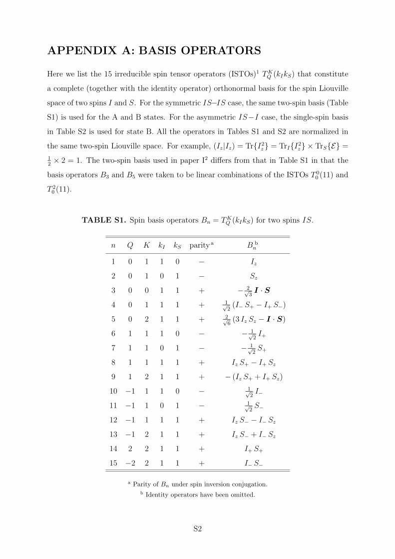
APPENDIX A: BASIS OPERATORS

Here we list the 15 irreducible spin tensor operators (ISTOs)1 TKQ (kIkS) that constitute

a complete (together with the identity operator) orthonormal basis for the spin Liouville

space of two spins I and S. For the symmetric IS−IS case, the same two-spin basis (Table

S1) is used for the A and B states. For the asymmetric IS−I case, the single-spin basis

in Table S2 is used for state B. All the operators in Tables S1 and S2 are normalized in

the same two-spin Liouville space. For example, (Iz|Iz) = TrI2z = TrII2

z × TrSE =

12× 2 = 1. The two-spin basis used in paper I2 differs from that in Table S1 in that the

basis operators B3 and B5 were taken to be linear combinations of the ISTOs T 00 (11) and

T 20 (11).

TABLE S1. Spin basis operators Bn = TKQ (kIkS) for two spins IS.

n Q K kI kS parity a B bn

1 0 1 1 0 − Iz

2 0 1 0 1 − Sz

3 0 0 1 1 + − 2√3I · S

4 0 1 1 1 + 1√2

(I− S+ − I+ S−)

5 0 2 1 1 + 2√6

(3 Iz Sz − I · S)

6 1 1 1 0 − − 1√2I+

7 1 1 0 1 − − 1√2S+

8 1 1 1 1 + Iz S+ − I+ Sz

9 1 2 1 1 + − (Iz S+ + I+ Sz)

10 −1 1 1 0 − 1√2I−

11 −1 1 0 1 − 1√2S−

12 −1 1 1 1 + Iz S− − I− Sz13 −1 2 1 1 + Iz S− + I− Sz

14 2 2 1 1 + I+ S+

15 −2 2 1 1 + I− S−

a Parity of Bn under spin inversion conjugation.b Identity operators have been omitted.

S2

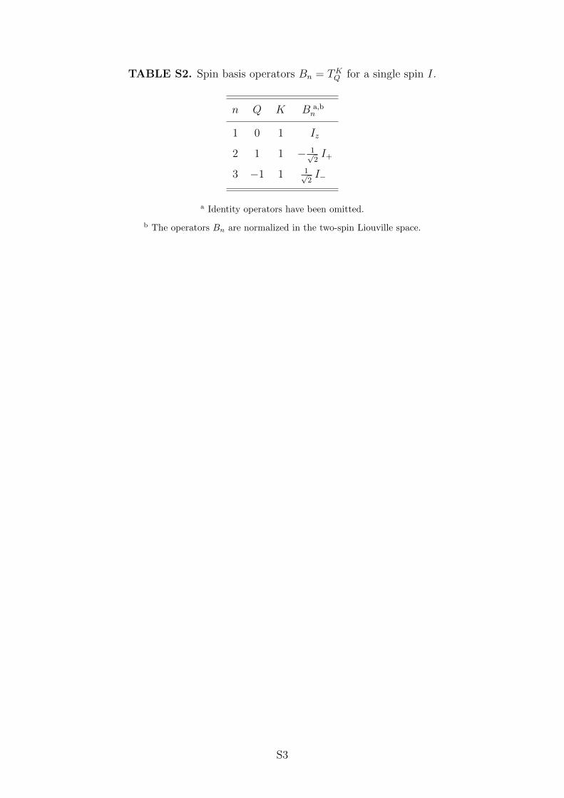
TABLE S2. Spin basis operators Bn = TKQ for a single spin I.

n Q K B a,bn

1 0 1 Iz

2 1 1 − 1√2I+

3 −1 1 1√2I−

a Identity operators have been omitted.

b The operators Bn are normalized in the two-spin Liouville space.

S3

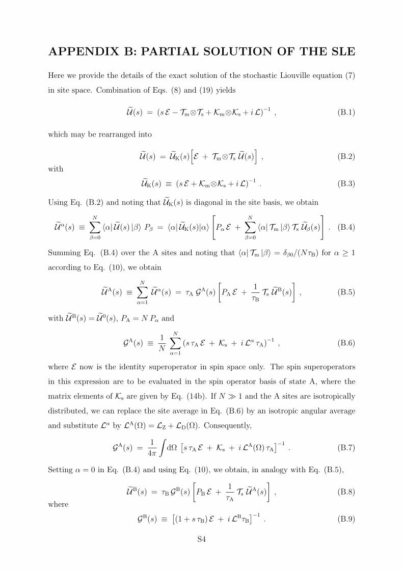
APPENDIX B: PARTIAL SOLUTION OF THE SLE

Here we provide the details of the exact solution of the stochastic Liouville equation (7)

in site space. Combination of Eqs. (8) and (19) yields

U(s) = (s E − Tm⊗Ts +Km⊗Ks + iL)−1 , (B.1)

which may be rearranged into

U(s) = UK(s)[E + Tm⊗Ts U(s)

], (B.2)

with

UK(s) ≡ (s E +Km⊗Ks + iL)−1 . (B.3)

Using Eq. (B.2) and noting that UK(s) is diagonal in the site basis, we obtain

Uα(s) ≡N∑β=0

〈α| U(s) |β〉 Pβ = 〈α| UK(s)|α〉

[Pα E +

N∑β=0

〈α| Tm |β〉 Ts Uβ(s)

]. (B.4)

Summing Eq. (B.4) over the A sites and noting that 〈α| Tm |β〉 = δβ0/(NτB) for α ≥ 1

according to Eq. (10), we obtain

UA(s) ≡N∑α=1

Uα(s) = τA GA(s)

[PA E +

1

τB

Ts UB(s)

], (B.5)

with UB(s) = U0(s), PA = N Pα and

GA(s) ≡ 1

N

N∑α=1

(s τA E + Ks + iLα τA)−1 , (B.6)

where E now is the identity superoperator in spin space only. The spin superoperators

in this expression are to be evaluated in the spin operator basis of state A, where the

matrix elements of Ks are given by Eq. (14b). If N 1 and the A sites are isotropically

distributed, we can replace the site average in Eq. (B.6) by an isotropic angular average

and substitute Lα by LA(Ω) = LZ + LD(Ω). Consequently,

GA(s) =1

4π

∫dΩ

[s τA E + Ks + iLA(Ω) τA

]−1. (B.7)

Setting α = 0 in Eq. (B.4) and using Eq. (10), we obtain, in analogy with Eq. (B.5),

UB(s) = τB GB(s)

[PB E +

1

τA

Ts UA(s)

], (B.8)

where

GB(s) ≡[(1 + s τB) E + iLBτB

]−1. (B.9)

S4

Equations (B.5) and (B.8) can now be solved for the two unknowns, with the result

UA(s) = τA

[E − GA(s) Ts GB(s) Ts

]−1 GA(s)[PA E + PB Ts GB(s)

], (B.10a)

UB(s) = τB

[E − GB(s) Ts GA(s) Ts

]−1 GB(s)[PB E + PA Ts GA(s)

]. (B.10b)

which allows us to obtain the site-averaged resolvent as

⟨U(s)

⟩= UA(s) + UB(s) . (B.11)

The superoperator⟨U(s)

⟩acts in a composite spin Liouville space of dimension D =

DB + DA. In Eq. (25), we partitioned the D ×D supermatrix representations of⟨U(s)

⟩into four blocks. To express Eq. (B.10) in terms of partitioned matrices, we partition the

identity matrix as

E →

1B 0

0 1A

, (B.12)

where 1B and 1A are DB × DB and DA × DA identity matrices, respectively, and 0 is a

DB ×DA or DA ×DB null matrix. According to Eq. (13),

Ts →

0 T

T′ 0

, (B.13)

where the DB ×DA matrix T (and its transpose T′) was defined in connection with Eq.

(15). Furthermore,

GB(s) →

GB(s) 0

0 0

, (B.14)

where, according to Eq. (B.9),

GB(s) =[(1 + s τB)1B + iLBτB

]−1. (B.15)

Finally,

GA(s) →

0 0

0 GA(s)

, (B.16)

where, according to Eq. (B.7),

GA(s) =1

4π

∫dΩ

[s τA 1A + K + iLA(Ω) τA

]−1, (B.17)

and the DA ×DA matrix K is diagonal with elements [1−∆K(nA)].

S5

Substituting these partitioned matrices into Eq. (B.10) and using Eq. (B.11), we can

express⟨U(s)

⟩on the block form introduced in Eq. (25),

⟨U(s)

⟩=

UBB

(s) UBA

(s)

UAB

(s) UAA

(s)

, (B.18)

with the submatrices given by Eq. (28) of the main text.

S6

APPENDIX C: INTEGRAL RELAXATION RATE

1. Asymmetric exchange

Here we simplify the expressions for the integral relaxation rate for the IS−I case by

expressing the matrix elements UXYnp ≡ (n|U

XY(0)|p) appearing in Eqs. (39) – (41) in

terms of the elements gnp ≡ (n|GA(0)|p) of the supermatrix GA(0) in Eq. (30).

We consider first the submatrix UBB

(0). Combining Eqs. (28a) and (29) and the

detailed balance relation PBτA = PAτB, we obtain

UBB

(0) =P 2

B τA

PA

[1B + iLB τB −TGA(0)T′]−1

. (C.1)

Because the matrix GA(0) is isotropically averaged, it must reflect the axial symmetry of

the spin system in the external magnetic field. According to the Wigner-Eckart theorem,1

GA(0) must then be block-diagonal in the ISTO basis of Table S1, with one 5× 5 block

(Q = 0), two 4 × 4 blocks (Q = ±1) and two 1 × 1 blocks (Q = ±2). Pre and post-

multiplication by the matrix T in Eq. (16) picks out the first diagonal element in each of

the first three blocks (Q = 0, ±1) to give

TGA(0)T′ =

g11 0 0

0 g66 0

0 0 g10,10

. (C.2)

The Liouvillian for the B state, with only a Zeeman coupling, is

LB = ωI

0 0 0

0 1 0

0 0 −1

. (C.3)

Combination of Eqs. (C.1) – (C.3) yields

UBB

(0) =P 2

B τA

PA

(1− g11)−1 0 0

0 (1− g66 + i ωIτB)−1 0

0 0 (1− g10,10 − i ωIτB)−1

, (C.4)

so that

UBB11 =

P 2B τA

PA(1− g11). (C.5)

S7

Comparison of Eqs. (28a) and (28b) shows that

UBA

(0) =PA

PB

UBB

(0)TGA(0) . (C.6)

Using Eqs. (16) and (C.4), we thus obtain

UBA11 =

PA

PB

UBB11 g11 =

PB τA g11

1− g11

, (C.7a)

UBA12 =

PA

PB

UBB11 g12 =

PB τA g12

1− g11

. (C.7b)

Next, we consider the submatrix UAA

(0) in Eq. (28d). Like GA(0) it is block-diagonal,

so we need only retain the Q = 0 block. From Eqs. (16), (29) and (C.3), it follows that

in the Q = 0 block of the matrix T′GB(0)T all elements are 0, except the (11) element

which is 1. Consequently,

[GA(0)T′ GB(0)T]Q=0 =

g11 0 0 0 0

g21 0 0 0 0

g31 0 0 0 0

g41 0 0 0 0

g51 0 0 0 0

, (C.8)

and

[1A −GA(0)T′ GB(0)T]−1Q=0 =

1− g11 0 0 0 0

−g21 1 0 0 0

−g31 0 1 0 0

−g41 0 0 1 0

−g51 0 0 0 1

−1

=

11−g11 0 0 0 0

g211−g11 1 0 0 0

g311−g11 0 1 0 0

g411−g11 0 0 1 0

g511−g11 0 0 0 1

.

(C.9)

Combination of Eqs. (28d) and (C.9) now yields

UAA11 = PA τA

g11

1− g11

, (C.10a)

UAA12 = PA τA

g12

1− g11

, (C.10b)

UAA21 = PA τA

g21

1− g11

, (C.10c)

UAA22 = PA τA

[g12 g21

1− g11

+ g22

]. (C.10d)

S8

Finally, comparison of Eqs. (28c) and (28d) shows that

UAB

(0) =PB

PA

UAA

(0)T′GB(0) . (C.11)

It follows from Eqs. (16), (29) and (C.3) that the first column of the 15 × 3 matrix

T′ GB(0) has the first element equal to 1 and all others equal to 0. We then obtain from

Eqs. (C.10) and (C.11),

UAB11 =

PB

PA

UAA11 = PB τA

g11

1− g11

, (C.12a)

UAB21 =

PB

PA

UAA21 = PB τA

g21

1− g11

. (C.12b)

With the aid of Eqs. (C.5), (C.7), (C.10) and (C.12), we can now express the integral

relaxation rate in Eqs. (39) and (40) in terms of the matrix elements gnp. Noting that

PB + PA = 1, we obtain

R non1,I =

PA

τA

(1− g11)

P 2B + PA[(1 + PB) g11 + κ g12]

, (C.13a)

R non1,S =

PA

τA

κ (1− g11)

g21 + κPA[(1− g11) g22 + g12 g21], (C.13b)

and

R sel1,I =

PA

τA

(1− g11)

P 2B + PA(1 + PB) g11

, (C.14a)

R sel1,S =

1

τA

(1− g11)

(1− g11) g22 + g12 g21

. (C.14b)

In the dilute regime, where PA 1 and PB ≈ 1, the integral relaxation rate in Eqs.

(C.13) and (C.14a) reduce to

Rdil/non1,I = R

dil/sel1,I =

PA

τA

(1− g11) , (C.15)

and

Rdil/non1,S =

PA

τA

κ (1− g11)

g21

. (C.16)

S9

2. Symmetric exchange

For convenience, we collect here expressions for the integral relaxation rates analogous to

those given in Sec. II E.2, but for the symmetric IS−IS case. Most of these expressions

were presented in paper I using a somewhat different notation.

With the spin modes indexed according to Table S1, Eq. (34) yields

R1,I =PB η

B1 + PA η

A1

σB1 (0) + σA

1 (0), (C.17a)

R1,S =PB η

B2 + PA η

A2

σB2 (0) + σA

2 (0). (C.17b)

R1,IS =PB(ηB

1 + ηB2 ) + PA(ηA

1 + ηA2 )

σB1 (0) + σB

2 (0) + σA1 (0) + σA

2 (0), (C.17c)

where R1,IS is the integral relaxation rate associated with the total longitudinal magne-

tization of the two spins (in practice, relevant only for homonuclear spins).

For nonselective excitation, the initial conditions are

ηAn = ηB

n = δn1 + κ δn2 , (C.18)

so Eqs. (C.17) and (35) yield

R non1,I = [UBB

11 + UBA11 + UAB

11 + UAA11 + κ (UBB

12 + UBA12 + UAB

12 + UAA12 )]−1 , (C.19a)

R non1,S = κ [UBB

21 + UBA21 + UAB

21 + UAA21 + κ (UBB

22 + UBA22 + UAB

22 + UAA22 )]−1 , (C.19b)

R non1,IS = (1 + κ) [UBB

11 + UBB21 + UBA

11 + UBA21 + UAB

11 + UAB21 + UAA

11 + UAA21

+ κ (UBB12 + UBB

22 + UBA12 + UBA

22 + UAB12 + UAB

22 + UAA12 + UAA

22 )]−1. (C.19c)

In the dilute regime, Eq. (37) allows us to simplify Eq. (C.19) to

Rdil/non1,I =

1

UBB11 + κUBB

12

, (C.20a)

Rdil/non1,S =

κ

UBB21 + κUBB

22

, (C.20b)

Rdil/non1,IS =

(1 + κ)

UBB11 + UBB

21 + κ (UBB12 + UBB

22 ). (C.20c)

S10

For selective excitation of spin I, the initial conditions are

ηAn = ηB

n = δn1 , (C.21)

so Eqs. (C.17a) and (35) yield

R sel1,I = [UBB

11 + UBA11 + UAB

11 + UAA11 ]−1 , (C.22)

reducing in the dilute regime to

Rdil/sel1,I =

1

UBB11

. (C.23)

For selective excitation of spin S, the initial conditions are

ηAn = ηB

n = κ δn2 , (C.24)

so Eqs. (C.17b) and (35) yield

R sel1,S = [UBB

22 + UBA22 + UAB

22 + UAA22 ]−1 , (C.25)

reducing in the dilute regime to

Rdil/sel1,S =

1

UBB22

. (C.26)

S11

APPENDIX D: ZERO-FIELD REGIME

Here we derive analytical expressions, valid for the IS− I case in the zero-field (ZF)

regime, for the Laplace transform of the spin modes σA1 (t), σA

2 (t), σA4 (t) and σB

1 (t), with

the subscripts referring to the basis operators in Tables S1 and S2. We also obtain

analytical expressions, valid in the ZF regime, for the integral relaxation rates in Eqs.

(C.13) and (C.14).

In the ZF regime, state A can be described in the subspace spanned by the rank-1

zero-quantum operators B1, B2 and B4 in Table S1, so Eq. (25) can be written asσB

1 (s)

σA1 (s)

σA2 (s)

σA4 (s)

=

UBB(s) UBA

(s)

UAB

(s) UAA

(s)

ηB

1

ηA1

ηA2

ηA4

, (D.1)

with the resolvent submatrices given by Eq. (28), where GA now is a 3 × 3 matrix.

Furthermore, in the ZF regime, Eq. (29) reduces to

GB = (1 + s τB)−1 1B , (D.2)

with 1B the 3× 3 identity matrix, and Eq. (16) yields

T =

1 0 0

0 0 0

0 0 0

. (D.3)

Combining these results with Eq. (28), we obtain

UBB(s) =PB τB

(1− g11 + s τB), (D.4)

UBA

(s) =PA τB

(1− g11 + s τB)

[g11 g12 g14

], (D.5)

UAA

(s) = PA τA(1 + s τB)

(1− g11 + s τB)

g11 g12 g14

g21 G22 G24

g41 G42 G44

, (D.6)

S12

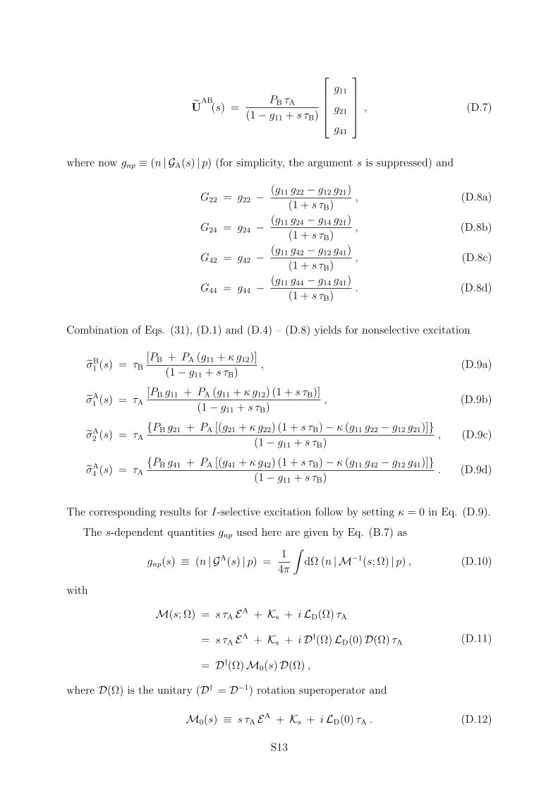
UAB

(s) =PB τA

(1− g11 + s τB)

g11

g21

g41

, (D.7)

where now gnp ≡ (n | GA(s) | p) (for simplicity, the argument s is suppressed) and

G22 = g22 −(g11 g22 − g12 g21)

(1 + s τB), (D.8a)

G24 = g24 −(g11 g24 − g14 g21)

(1 + s τB), (D.8b)

G42 = g42 −(g11 g42 − g12 g41)

(1 + s τB), (D.8c)

G44 = g44 −(g11 g44 − g14 g41)

(1 + s τB). (D.8d)

Combination of Eqs. (31), (D.1) and (D.4) – (D.8) yields for nonselective excitation

σB1 (s) = τB

[PB + PA (g11 + κ g12)]

(1− g11 + s τB), (D.9a)

σA1 (s) = τA

[PB g11 + PA (g11 + κ g12) (1 + s τB)]

(1− g11 + s τB), (D.9b)

σA2 (s) = τA

PB g21 + PA [(g21 + κ g22) (1 + s τB)− κ (g11 g22 − g12 g21)](1− g11 + s τB)

, (D.9c)

σA4 (s) = τA

PB g41 + PA [(g41 + κ g42) (1 + s τB)− κ (g11 g42 − g12 g41)](1− g11 + s τB)

. (D.9d)

The corresponding results for I-selective excitation follow by setting κ = 0 in Eq. (D.9).

The s-dependent quantities gnp used here are given by Eq. (B.7) as

gnp(s) ≡ (n | GA(s) | p) =1

4π

∫dΩ (n |M−1(s; Ω) | p) , (D.10)

with

M(s; Ω) = s τA EA + Ks + iLD(Ω) τA

= s τA EA + Ks + iD†(Ω)LD(0)D(Ω) τA

= D†(Ω)M0(s)D(Ω) ,

(D.11)

where D(Ω) is the unitary (D† = D−1) rotation superoperator and

M0(s) ≡ s τA EA + Ks + iLD(0) τA . (D.12)

S13

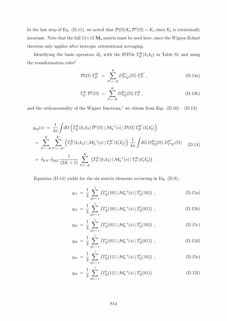
In the last step of Eq. (D.11), we noted that D(Ω)KsD†(Ω) = Ks since Ks is rotationally

invariant. Note that the full 15×15 M0 matrix must be used here, since the Wigner-Eckart

theorem only applies after isotropic orientational averaging.

Identifying the basis operators Bn with the ISTOs TKQ (k1k2) in Table S1 and using

the transformation rules1

D(Ω) TK′

Q′ =K∑

P ′=−K

DK′

P ′Q′(Ω) TK′

P ′ , (D.13a)

TKQ D†(Ω) =K∑

P=−K

DK∗PQ(Ω) TKP , (D.13b)

and the orthonormality of the Wigner functions,1 we obtain from Eqs. (D.10) – (D.13)

gnp(s) =1

4π

∫dΩ(TKQ (k1k2)D†(Ω) |M−1

0 (s) | D(Ω)TK′

Q′ (k′1k′2))

=K∑

P=−K

K′∑P ′=−K′

(TKP (k1k2) |M−1

0 (s) |TK′

P ′ (k′1k′2)) 1

4π

∫dΩDK∗

PQ(Ω)DK′

P ′Q′(Ω)

= δKK′ δQQ′1

(2K + 1)

K∑P=−K

(TKP (k1k2) |M−1

0 (s) |TKP (k′1k′2)).

(D.14)

Equation (D.14) yields for the six matrix elements occurring in Eq. (D.9),

g11 =1

3

1∑Q=−1

(T 1Q(10) |M−1

0 (s) |T 1Q(10)

), (D.15a)

g12 =1

3

1∑Q=−1

(T 1Q(10) |M−1

0 (s) |T 1Q(01)

), (D.15b)

g21 =1

3

1∑Q=−1

(T 1Q(01) |M−1

0 (s) |T 1Q(10)

), (D.15c)

g22 =1

3

1∑Q=−1

(T 1Q(01) |M−1

0 (s) |T 1Q(01)

), (D.15d)

g41 =1

3

1∑Q=−1

(T 1Q(11) |M−1

0 (s) |T 1Q(10)

), (D.15e)

g42 =1

3

1∑Q=−1

(T 1Q(11) |M−1

0 (s) |T 1Q(01)

). (D.15f)

S14

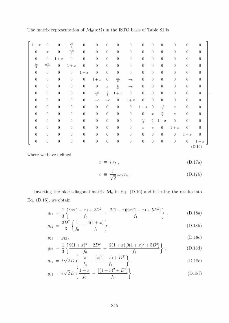
The matrix representation of M0(s; Ω) in the ISTO basis of Table S1 is

1 + x 0 0 2c3 0 0 0 0 0 0 0 0 0 0 0

0 x 0 −2c3 0 0 0 0 0 0 0 0 0 0 0

0 0 1 + x 0 0 0 0 0 0 0 0 0 0 0 0

2c3

−2c3 0 1 + x 0 0 0 0 0 0 0 0 0 0 0

0 0 0 0 1 + x 0 0 0 0 0 0 0 0 0 0

0 0 0 0 0 1 + x 0 −c3 −c 0 0 0 0 0 0

0 0 0 0 0 0 x c3 −c 0 0 0 0 0 0

0 0 0 0 0 −c3

c3 1 + x 0 0 0 0 0 0 0

0 0 0 0 0 −c −c 0 1 + x 0 0 0 0 0 0

0 0 0 0 0 0 0 0 0 1 + x 0 −c3 c 0 0

0 0 0 0 0 0 0 0 0 0 x c3 c 0 0

0 0 0 0 0 0 0 0 0 −c3

c3 1 + x 0 0 0

0 0 0 0 0 0 0 0 0 c c 0 1 + x 0 0

0 0 0 0 0 0 0 0 0 0 0 0 0 1 + x 0

0 0 0 0 0 0 0 0 0 0 0 0 0 0 1 + x

,

(D.16)

where we have defined

x ≡ s τA , (D.17a)

c ≡ i√2ωD τA . (D.17b)

Inverting the block-diagonal matrix M0 in Eq. (D.16) and inserting the results into

Eq. (D.15), we obtain

g11 =1

3

9x(1 + x) + 2D2

f0

+2(1 + x)[9x(1 + x) + 5D2]

f1

, (D.18a)

g12 =2D2

3

1

f0

− 4(1 + x)

f1

, (D.18b)

g21 = g12 , (D.18c)

g22 =1

3

9(1 + x)2 + 2D2

f0

+2(1 + x)[9(1 + x)2 + 5D2]

f1

, (D.18d)

g41 = i√

2D

− xf0

+[x(1 + x) +D2]

f1

, (D.18e)

g42 = i√

2D

1 + x

f0

− [(1 + x)2 +D2]

f1

, (D.18f)

S15

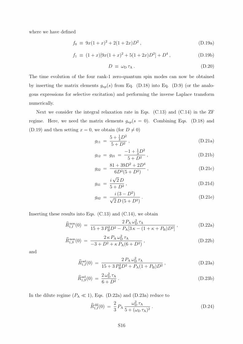
where we have defined

f0 ≡ 9x(1 + x)2 + 2(1 + 2x)D2 , (D.19a)

f1 ≡ (1 + x)[9x(1 + x)2 + 5(1 + 2x)D2] +D4 , (D.19b)

D ≡ ωD τA . (D.20)

The time evolution of the four rank-1 zero-quantum spin modes can now be obtained

by inserting the matrix elements gnp(s) from Eq. (D.18) into Eq. (D.9) (or the analo-

gous expressions for selective excitation) and performing the inverse Laplace transform

numerically.

Next we consider the integral relaxation rate in Eqs. (C.13) and (C.14) in the ZF

regime. Here, we need the matrix elements gnp(s = 0). Combining Eqs. (D.18) and

(D.19) and then setting x = 0, we obtain (for D 6= 0)

g11 =5 + 1

3D2

5 +D2, (D.21a)

g12 = g21 =−1 + 1

3D2

5 +D2, (D.21b)

g22 =81 + 39D2 + 2D4

6D2(5 +D2), (D.21c)

g41 =i√

2D

5 +D2, (D.21d)

g42 =i (3−D2)√2D (5 +D2)

. (D.21e)

Inserting these results into Eqs. (C.13) and (C.14), we obtain

R non1,I (0) =

2PA ω2D τA

15 + 3P 2BD

2 − PA[3κ− (1 + κ+ PB)D2], (D.22a)

R non1,S (0) =

2κPA ω2D τA

−3 +D2 + κPA(6 +D2), (D.22b)

and

R sel1,I(0) =

2PA ω2D τA

15 + 3P 2BD

2 + PA(1 + PB)D2, (D.23a)

R sel1,S(0) =

2ω2D τA

6 +D2. (D.23b)

In the dilute regime (PA 1), Eqs. (D.22a) and (D.23a) reduce to

R dil1,I(0) =

2

3PA

ω2D τA

5 + (ωD τA)2. (D.24)

S16

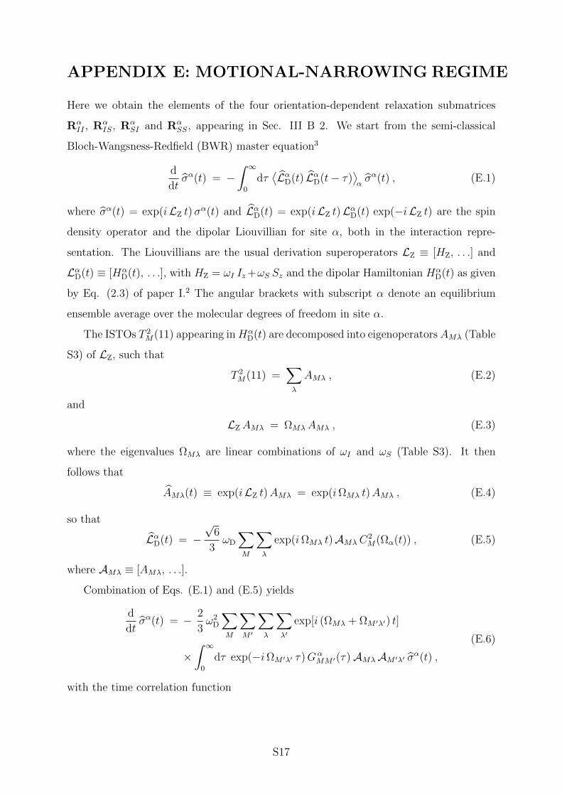
APPENDIX E: MOTIONAL-NARROWINGREGIME

Here we obtain the elements of the four orientation-dependent relaxation submatrices

RαII , Rα

IS, RαSI and Rα

SS, appearing in Sec. III B 2. We start from the semi-classical

Bloch-Wangsness-Redfield (BWR) master equation3

d

dtσα(t) = −

∫ ∞0

dτ⟨LαD(t) LαD(t− τ)

⟩ασα(t) , (E.1)

where σα(t) = exp(iLZ t)σα(t) and LαD(t) = exp(iLZ t)LαD(t) exp(−iLZ t) are the spin

density operator and the dipolar Liouvillian for site α, both in the interaction repre-

sentation. The Liouvillians are the usual derivation superoperators LZ ≡ [HZ, . . .] and

LαD(t) ≡ [HαD(t), . . .], with HZ = ωI Iz+ωS Sz and the dipolar Hamiltonian Hα

D(t) as given

by Eq. (2.3) of paper I.2 The angular brackets with subscript α denote an equilibrium

ensemble average over the molecular degrees of freedom in site α.

The ISTOs T 2M(11) appearing inHα

D(t) are decomposed into eigenoperatorsAMλ (Table

S3) of LZ, such that

T 2M(11) =

∑λ

AMλ , (E.2)

and

LZAMλ = ΩMλAMλ , (E.3)

where the eigenvalues ΩMλ are linear combinations of ωI and ωS (Table S3). It then

follows that

AMλ(t) ≡ exp(iLZ t)AMλ = exp(iΩMλ t)AMλ , (E.4)

so that

LαD(t) = −√

6

3ωD

∑M

∑λ

exp(iΩMλ t)AMλC2M(Ωα(t)) , (E.5)

where AMλ ≡ [AMλ, . . .].

Combination of Eqs. (E.1) and (E.5) yields

d

dtσα(t) = − 2

3ω2

D

∑M

∑M ′

∑λ

∑λ′

exp[i (ΩMλ + ΩM ′λ′) t]

×∫ ∞

0

dτ exp(−iΩM ′λ′ τ)GαMM ′(τ)AMλAM ′λ′ σ

α(t) ,

(E.6)

with the time correlation function

S17

TABLE S3. Eigenoperators and eigenvalues of LZ.

M λ AMλ ΩMλ

0 1 4√6Iz Sz 0

0 2 − 1√6I− S+ ωS − ωI

0 3 − 1√6I+ S− ωI − ωS

1 1 − Iz S+ ωS

1 2 − I+ Sz ωI

-1 1 Iz S− −ωS-1 2 I− Sz −ωI2 1 I+ S+ ωI + ωS

-2 1 I− S− −ωI − ωS

GαMM ′(τ) ≡

⟨C 2M(Ωα(0))C 2

M ′(Ωα(τ))⟩α

= C 2M(Ωα(0))

∫dΩα(τ) f(Ωα(τ) |Ωα(0)) C 2

M ′(Ωα(τ)) ,

(E.7)

where the dipole vector orientation Ωα(τ) is modeled as a stationary random process.

Note that the time correlation function is not averaged over the initial orientation Ωα(0),

which is fixed by the nuclear geometry in site α. In the EMOR model, the orientation of

the dipole vector is randomized upon exchange, as expressed by the propagator

f(Ωα(τ) |Ωα(0)) =1

4π+

[δ(Ωα(τ)− Ωα(0)) − 1

4π

]exp(−τ/τA) , (E.8)

where τA is the mean survival time in the site. Combining Eqs. (E.7) and (E.8) and

making use of the orthogonality of the spherical harmonics C2M(Ωα),1 we find

GαMM ′(τ) = FMM ′(Ωα) exp(−τ/τA) , (E.9)

with

FMM ′(Ωα) ≡ C 2M(Ωα)C 2

M ′(Ωα) = d 2M0(β) d 2

M ′0(β) exp[i(M +M ′)α] . (E.10)

With the time correlation function (E.9), we can write the master equation (E.6) as

d

dtσα(t) = −Rα(t) σα(t) . (E.11)

S18

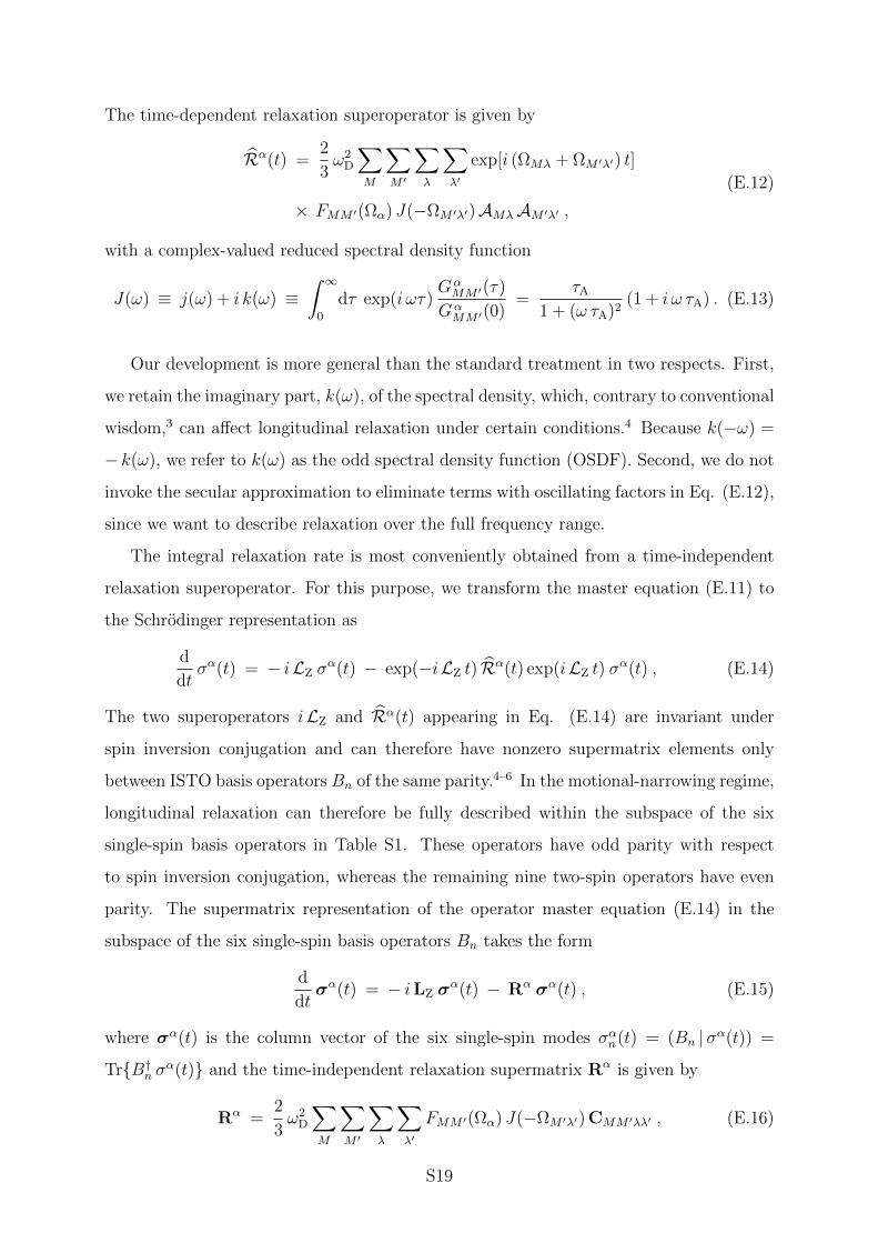
The time-dependent relaxation superoperator is given by

Rα(t) =2

3ω2

D

∑M

∑M ′

∑λ

∑λ′

exp[i (ΩMλ + ΩM ′λ′) t]

× FMM ′(Ωα) J(−ΩM ′λ′)AMλAM ′λ′ ,

(E.12)

with a complex-valued reduced spectral density function

J(ω) ≡ j(ω) + i k(ω) ≡∫ ∞

0

dτ exp(i ωτ)GαMM ′(τ)

GαMM ′(0)

=τA

1 + (ω τA)2(1 + i ω τA) . (E.13)

Our development is more general than the standard treatment in two respects. First,

we retain the imaginary part, k(ω), of the spectral density, which, contrary to conventional

wisdom,3 can affect longitudinal relaxation under certain conditions.4 Because k(−ω) =

− k(ω), we refer to k(ω) as the odd spectral density function (OSDF). Second, we do not

invoke the secular approximation to eliminate terms with oscillating factors in Eq. (E.12),

since we want to describe relaxation over the full frequency range.

The integral relaxation rate is most conveniently obtained from a time-independent

relaxation superoperator. For this purpose, we transform the master equation (E.11) to

the Schrodinger representation as

d

dtσα(t) = − iLZ σ

α(t) − exp(−iLZ t) Rα(t) exp(iLZ t) σα(t) , (E.14)

The two superoperators iLZ and Rα(t) appearing in Eq. (E.14) are invariant under

spin inversion conjugation and can therefore have nonzero supermatrix elements only

between ISTO basis operators Bn of the same parity.4–6 In the motional-narrowing regime,

longitudinal relaxation can therefore be fully described within the subspace of the six

single-spin basis operators in Table S1. These operators have odd parity with respect

to spin inversion conjugation, whereas the remaining nine two-spin operators have even

parity. The supermatrix representation of the operator master equation (E.14) in the

subspace of the six single-spin basis operators Bn takes the form

d

dtσα(t) = − iLZ σ

α(t) − Rα σα(t) , (E.15)

where σα(t) is the column vector of the six single-spin modes σαn(t) = (Bn |σα(t)) =

TrB†n σα(t) and the time-independent relaxation supermatrix Rα is given by

Rα =2

3ω2

D

∑M

∑M ′

∑λ

∑λ′

FMM ′(Ωα) J(−ΩM ′λ′)CMM ′λλ′ , (E.16)

S19

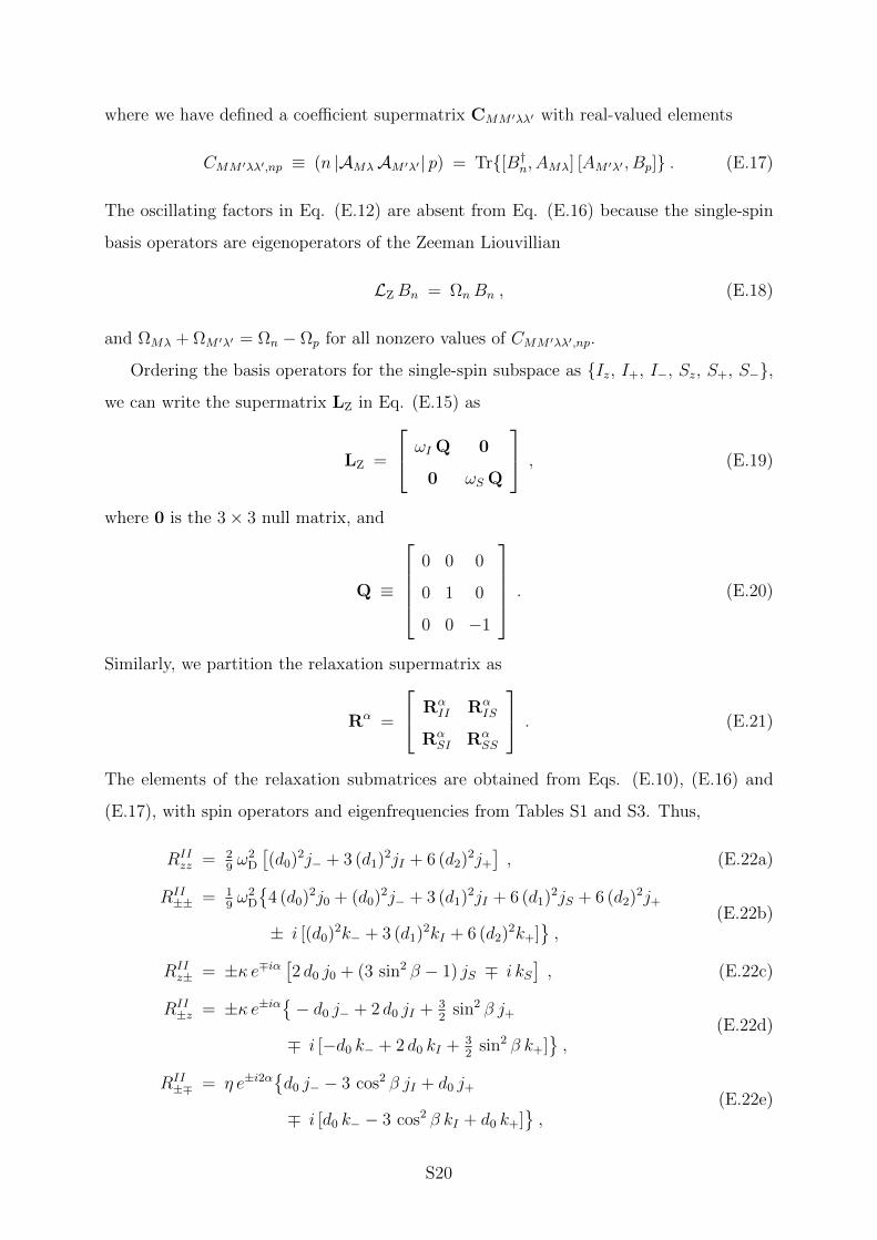
where we have defined a coefficient supermatrix CMM ′λλ′ with real-valued elements

CMM ′λλ′,np ≡ (n |AMλAM ′λ′| p) = Tr[B†n, AMλ] [AM ′λ′ , Bp] . (E.17)

The oscillating factors in Eq. (E.12) are absent from Eq. (E.16) because the single-spin

basis operators are eigenoperators of the Zeeman Liouvillian

LZ Bn = ΩnBn , (E.18)

and ΩMλ + ΩM ′λ′ = Ωn − Ωp for all nonzero values of CMM ′λλ′,np.

Ordering the basis operators for the single-spin subspace as Iz, I+, I−, Sz, S+, S−,

we can write the supermatrix LZ in Eq. (E.15) as

LZ =

ωI Q 0

0 ωS Q

, (E.19)

where 0 is the 3× 3 null matrix, and

Q ≡

0 0 0

0 1 0

0 0 −1

. (E.20)

Similarly, we partition the relaxation supermatrix as

Rα =

RαII Rα

IS

RαSI Rα

SS

. (E.21)

The elements of the relaxation submatrices are obtained from Eqs. (E.10), (E.16) and

(E.17), with spin operators and eigenfrequencies from Tables S1 and S3. Thus,

RIIzz = 2

9ω2

D

[(d0)2j− + 3 (d1)2jI + 6 (d2)2j+

], (E.22a)

RII±± = 1

9ω2

D

4 (d0)2j0 + (d0)2j− + 3 (d1)2jI + 6 (d1)2jS + 6 (d2)2j+

± i [(d0)2k− + 3 (d1)2kI + 6 (d2)2k+],

(E.22b)

RIIz± = ±κ e∓iα

[2 d0 j0 + (3 sin2 β − 1) jS ∓ i kS

], (E.22c)

RII±z = ±κ e±iα

− d0 j− + 2 d0 jI + 3

2sin2 β j+

∓ i [−d0 k− + 2 d0 kI + 32

sin2 β k+],

(E.22d)

RII±∓ = η e±i2α

d0 j− − 3 cos2 β jI + d0 j+

∓ i [d0 k− − 3 cos2 β kI + d0 k+],

(E.22e)

S20

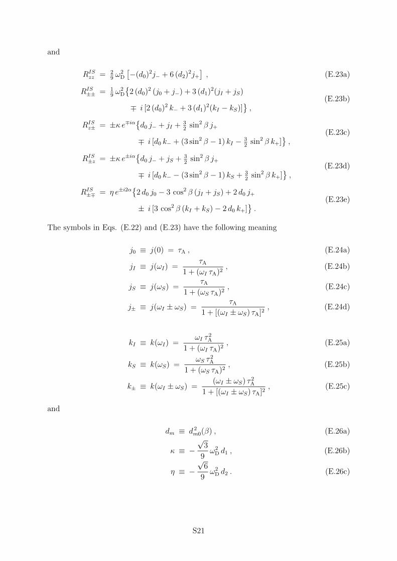
and

RISzz = 2

9ω2

D

[−(d0)2j− + 6 (d2)2j+

], (E.23a)

RIS±± = 1

9ω2

D

2 (d0)2 (j0 + j−) + 3 (d1)2(jI + jS)

∓ i [2 (d0)2 k− + 3 (d1)2(kI − kS)],

(E.23b)

RISz± = ±κ e∓iα

d0 j− + jI + 3

2sin2 β j+

∓ i [d0 k− + (3 sin2 β − 1) kI − 32

sin2 β k+],

(E.23c)

RIS±z = ±κ e±iα

d0 j− + jS + 3

2sin2 β j+

∓ i [d0 k− − (3 sin2 β − 1) kS + 32

sin2 β k+],

(E.23d)

RIS±∓ = η e±i2α

2 d0 j0 − 3 cos2 β (jI + jS) + 2 d0 j+

± i [3 cos2 β (kI + kS)− 2 d0 k+].

(E.23e)

The symbols in Eqs. (E.22) and (E.23) have the following meaning

j0 ≡ j(0) = τA , (E.24a)

jI ≡ j(ωI) =τA

1 + (ωI τA)2, (E.24b)

jS ≡ j(ωS) =τA

1 + (ωS τA)2, (E.24c)

j± ≡ j(ωI ± ωS) =τA

1 + [(ωI ± ωS) τA]2, (E.24d)

kI ≡ k(ωI) =ωI τ

2A

1 + (ωI τA)2, (E.25a)

kS ≡ k(ωS) =ωS τ

2A

1 + (ωS τA)2, (E.25b)

k± ≡ k(ωI ± ωS) =(ωI ± ωS) τ 2

A

1 + [(ωI ± ωS) τA]2, (E.25c)

and

dm ≡ d 2m0(β) , (E.26a)

κ ≡ −√

3

9ω2

D d1 , (E.26b)

η ≡ −√

6

9ω2

D d2 . (E.26c)

S21

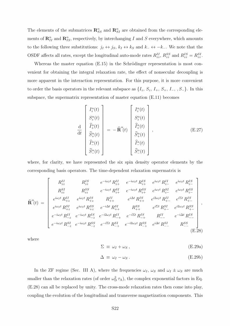
The elements of the submatrices RαSS and Rα

SI are obtained from the corresponding ele-

ments of RαII and Rα

IS, respectively, by interchanging I and S everywhere, which amounts

to the following three substitutions: jI ↔ jS, kI ↔ kS and k− ↔ −k−. We note that the

OSDF affects all rates, except the longitudinal auto-mode rates RIIzz, R

SSzz and RIS

zz = RSIzz .

Whereas the master equation (E.15) in the Schrodinger representation is most con-

venient for obtaining the integral relaxation rate, the effect of nonsecular decoupling is

more apparent in the interaction representation. For this purpose, it is more convenient

to order the basis operators in the relevant subspace as Iz, Sz, I+, S+, I−, , S−. In this

subspace, the supermatrix representation of master equation (E.11) becomes

d

dt

Iαz (t)

Sαz (t)

Iα+(t)

Sα+(t)

Iα−(t)

Sα−(t)

= − R

α(t)

Iαz (t)

Sαz (t)

Iα+(t)

Sα+(t)

Iα−(t)

Sα−(t)

, (E.27)

where, for clarity, we have represented the six spin density operator elements by the

corresponding basis operators. The time-dependent relaxation supermatrix is

Rα(t) =

RIIzz RIS

zz e−iωI tRIIz+ e−iωStRIS

z+ eiωI tRIIz− eiωStRIS

z−

RSIzz RSS

zz e−iωI tRSIz+ e−iωStRSS

z+ eiωI tRSIz− eiωStRSS

z−

eiωI tRII+z eiωI tRIS

+z RII++ ei∆tRIS

++ ei2ωI tRII+− eiΣtRIS

+−

eiωStRSI+z eiωStRSS

+z e−i∆tRSI++ RSS

++ eiΣtRSI+− ei2ωStRSS

+−

e−iωI tRII−z e−iωI tRIS

−z e−i2ωI tRII−+ e−iΣtRIS

−+ RII−− e−i∆tRIS

−−

e−iωStRSI−z e−iωStRSS

−z e−iΣtRSI−+ e−i2ωStRSS

−+ ei∆tRSI−− RSS

−−

,

(E.28)

where

Σ ≡ ωI + ωS , (E.29a)

∆ ≡ ωI − ωS . (E.29b)

In the ZF regime (Sec. III A), where the frequencies ωI , ωS and ωI ± ωS are much

smaller than the relaxation rates (of order ω2D τA), the complex exponential factors in Eq.

(E.28) can all be replaced by unity. The cross-mode relaxation rates then come into play,

coupling the evolution of the longitudinal and transverse magnetization components. This

S22

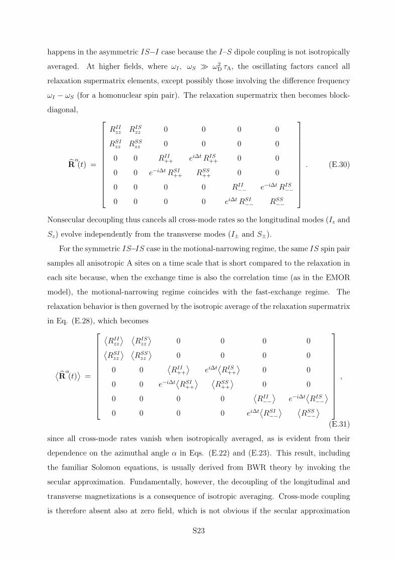
happens in the asymmetric IS−I case because the I–S dipole coupling is not isotropically

averaged. At higher fields, where ωI , ωS ω2D τA, the oscillating factors cancel all

relaxation supermatrix elements, except possibly those involving the difference frequency

ωI − ωS (for a homonuclear spin pair). The relaxation supermatrix then becomes block-

diagonal,

Rα(t) =

RIIzz RIS

zz 0 0 0 0

RSIzz RSS

zz 0 0 0 0

0 0 RII++ ei∆tRIS

++ 0 0

0 0 e−i∆tRSI++ RSS

++ 0 0

0 0 0 0 RII−− e−i∆tRIS

−−

0 0 0 0 ei∆tRSI−− RSS

−−

. (E.30)

Nonsecular decoupling thus cancels all cross-mode rates so the longitudinal modes (Iz and

Sz) evolve independently from the transverse modes (I± and S±).

For the symmetric IS−IS case in the motional-narrowing regime, the same IS spin pair

samples all anisotropic A sites on a time scale that is short compared to the relaxation in

each site because, when the exchange time is also the correlation time (as in the EMOR

model), the motional-narrowing regime coincides with the fast-exchange regime. The

relaxation behavior is then governed by the isotropic average of the relaxation supermatrix

in Eq. (E.28), which becomes

⟨Rα(t)⟩

=

⟨RIIzz

⟩ ⟨RISzz

⟩0 0 0 0⟨

RSIzz

⟩ ⟨RSSzz

⟩0 0 0 0

0 0⟨RII

++

⟩ei∆t⟨RIS

++

⟩0 0

0 0 e−i∆t⟨RSI

++

⟩ ⟨RSS

++

⟩0 0

0 0 0 0⟨RII−−⟩

e−i∆t⟨RIS−−⟩

0 0 0 0 ei∆t⟨RSI−−⟩ ⟨

RSS−−⟩

,

(E.31)

since all cross-mode rates vanish when isotropically averaged, as is evident from their

dependence on the azimuthal angle α in Eqs. (E.22) and (E.23). This result, including

the familiar Solomon equations, is usually derived from BWR theory by invoking the

secular approximation. Fundamentally, however, the decoupling of the longitudinal and

transverse magnetizations is a consequence of isotropic averaging. Cross-mode coupling

is therefore absent also at zero field, which is not obvious if the secular approximation

S23

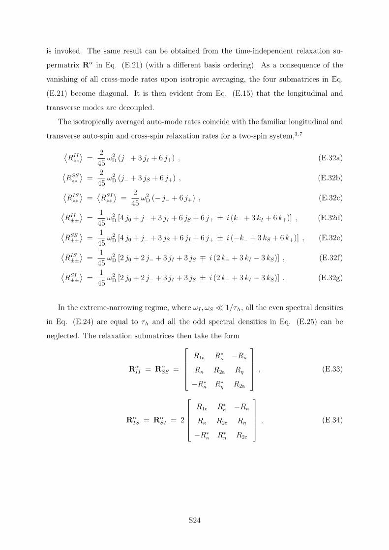
is invoked. The same result can be obtained from the time-independent relaxation su-

permatrix Rα in Eq. (E.21) (with a different basis ordering). As a consequence of the

vanishing of all cross-mode rates upon isotropic averaging, the four submatrices in Eq.

(E.21) become diagonal. It is then evident from Eq. (E.15) that the longitudinal and

transverse modes are decoupled.

The isotropically averaged auto-mode rates coincide with the familiar longitudinal and

transverse auto-spin and cross-spin relaxation rates for a two-spin system,3,7

⟨RIIzz

⟩=

2

45ω2

D (j− + 3 jI + 6 j+) , (E.32a)⟨RSSzz

⟩=

2

45ω2

D (j− + 3 jS + 6 j+) , (E.32b)⟨RISzz

⟩=⟨RSIzz

⟩=

2

45ω2

D (− j− + 6 j+) , (E.32c)⟨RII±±⟩

=1

45ω2

D [4 j0 + j− + 3 jI + 6 jS + 6 j+ ± i (k− + 3 kI + 6 k+)] , (E.32d)⟨RSS±±⟩

=1

45ω2

D [4 j0 + j− + 3 jS + 6 jI + 6 j+ ± i (−k− + 3 kS + 6 k+)] , (E.32e)⟨RIS±±⟩

=1

45ω2

D [2 j0 + 2 j− + 3 jI + 3 jS ∓ i (2 k− + 3 kI − 3 kS)] , (E.32f)⟨RSI±±⟩

=1

45ω2

D [2 j0 + 2 j− + 3 jI + 3 jS ± i (2 k− + 3 kI − 3 kS)] . (E.32g)

In the extreme-narrowing regime, where ωI , ωS 1/τA, all the even spectral densities

in Eq. (E.24) are equal to τA and all the odd spectral densities in Eq. (E.25) can be

neglected. The relaxation submatrices then take the form

RαII = Rα

SS =

R1a R∗κ −Rκ

Rκ R2a Rη

−R∗κ R∗η R2a

, (E.33)

RαIS = Rα

SI = 2

R1c R∗κ −Rκ

Rκ R2c Rη

−R∗κ R∗η R2c

, (E.34)

S24

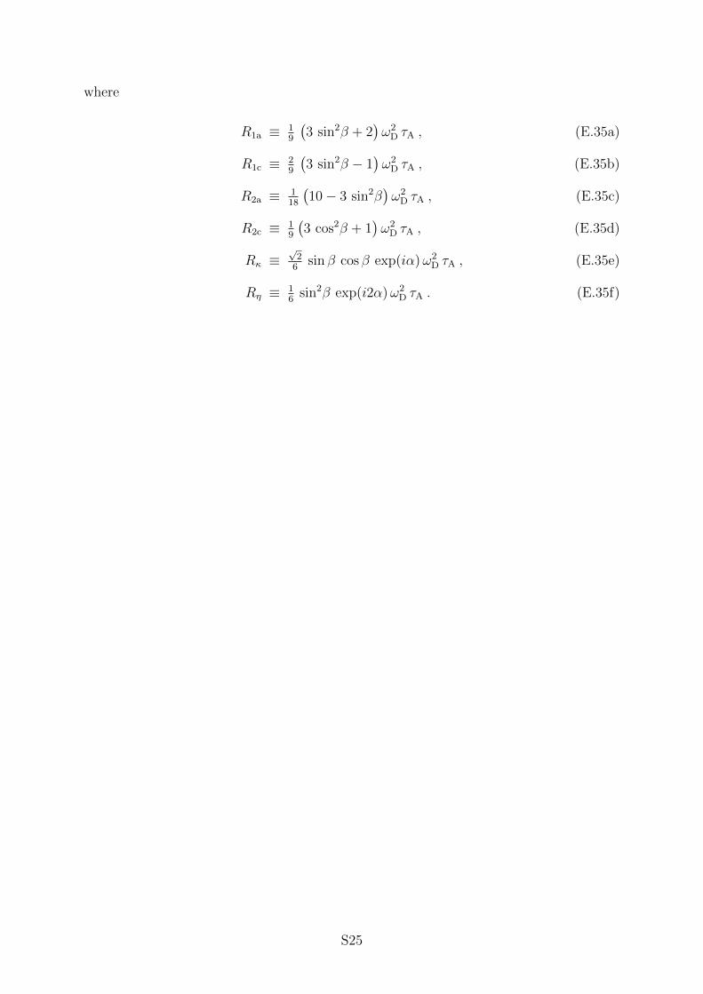
where

R1a ≡ 19

(3 sin2β + 2

)ω2

D τA , (E.35a)

R1c ≡ 29

(3 sin2β − 1

)ω2

D τA , (E.35b)

R2a ≡ 118

(10− 3 sin2β

)ω2

D τA , (E.35c)

R2c ≡ 19

(3 cos2β + 1

)ω2

D τA , (E.35d)

Rκ ≡√

26

sin β cos β exp(iα)ω2D τA , (E.35e)

Rη ≡ 16

sin2β exp(i2α)ω2D τA . (E.35f)

S25

APPENDIX F: TIME EVOLUTION OF Iz AND Sz

Here we derive analytical results for the time evolution of the longitudinal magnetiza-

tions in the ZF + MN regime, where only the spin modes σA1 = Iz and σA

2 = Sz are

coupled in state A. It must then be possible to describe the evolution of the longitudinal

magnetizations in the A and B states by three coupled equations:

d

dtIBz (t) = − 1

τB

IBz (t) +

1

τA

IAz (t) , (F.1a)

d

dtIAz (t) =

1

τB

IBz (t) −

(ρI +

1

τA

)IAz (t) − σIS S

Az (t) , (F.1b)

d

dtSAz (t) = −σSI IA

z (t) − ρS SAz (t) , (F.1c)

where, without loss of generality, we have set the equilibrium magnetizations to zero.

Apart from the exchange terms, Eqs. (F.1b) and (F1.c) have the same form as the two-

spin Solomon equations,3,8 but the four relaxation rates are not the same for the IS−I

EMOR model as for an isolated spin pair in isotropic solution. In the ZF regime, ρI = ρS

and σIS = σSI in the Solomon equations,3,8 but this symmetry is broken in the IS−I

EMOR model since only spin I can exchange with state B. For nonselective excitation,

Eq. (F.1) is to be solved subject to the initial conditions

IBz (0) = PB , IA

z (0) = SAz (0) = PA . (F.2)

The MN regime is also the fast-exchange regime, so 1/τA ρI , ρS, σIS, σSI . Because

exchange is much faster than auto-spin and cross-spin relaxation, the ratio of the Iz

magnetizations in states A and B remains at the initial value,

IAz (t)

IBz (t)

=IAz (0)

IBz (0)

=PA

PB

. (F.3)

When IAz (t) relaxes to the lattice (directly and via spin S), it is ‘immediately’ replen-

ished with magnetization from state B. Consequently, the total I-spin magnetization,

Iz(t) = IAz (t)+IB

z (t), relaxes slowly with an effective rate that is proportional to PA ω2D τA.

Summing Eqs. (F.1a) and (F.1b), we obtain

d

dtIz(t) = − ρI IA

z (t) − σIS SAz (t) . (F.4)

Substituting IAz (t) = PA Iz(t) from Eq. (F.3) into Eqs. (F.4) and (F.1c), we find

d

dtIz(t) = −PA ρI Iz(t) − σIS S

Az (t) , (F.5a)

d

dtSAz (t) = −PA σSI Iz(t) − ρS S

Az (t) . (F.5b)

S26

We shall consider Eq. (F.5) in two different time regimes. At short times, such that

t 1/(PA ω2D τA), the I and S spins are decoupled because the I spin has not yet relaxed.

We can then set Iz(t) = Iz(0) = 1 in Eq. (F.5b), whereby

d

dtSAz (t) = −σSI PA − ρS S

Az (t) = − ρS

[SAz (t) + PA

σSIρS

]. (F.6)

With SAz (0) = PA from Eq. (F.2), the solution to Eq. (F.6) is

SAz (t) = PA

[(1 +

σSIρS

)exp(−ρS t) −

σSIρS

]. (F.7)

The S-spin magnetization thus relaxes to a (negative) steady-state value, −PA σSI/ρS,

rather then to its zero equilibrium value.

After SAz (t) has reached its steady-state value while Iz(t) remains essentially constant,

both magnetizations relax together to zero at the same rate. This coupled evolution, on

the time scale t 1/ρS, is obtained by solving Eq. (F.5) subject to the initial conditions

Iz(0) = 1 , SAz (0) = −PA

σSIρS

. (F.8)

The solution is

Iz(t) =1

(λ+ − λ−)

[(ρS − λ−) Iz(0)− σIS SA

z (0)]

exp(−λ− t)

−[(ρS − λ+) Iz(0)− σIS SA

z (0)]

exp(−λ+ t),

(F.9a)

SAz (t) =

1

(λ+ − λ−)

[(PA ρI − λ−)SA

z (0)− PA σSI Iz(0)]

exp(−λ− t)

−[(PA ρI − λ+)SA

z (0)− PA σSI Iz(0)]

exp(−λ+ t),

(F.9b)

where

λ± ≡ 12

(ρS + PA ρI) ± 12

[(ρS − PA ρI)

2 + 4PA σIS σSI]1/2

. (F.10)

In the dilute regime, we can expand these rates as

λ+ = ρS + PAσIS σSIρS

+ O(P 2A) , (F.11a)

λ− = PA

(ρI −

σIS σSIρS

)+ O(P 2

A) . (F.11b)

Substitution from Eqs. (F.8) and (F.11) into Eq. (F.9) yields

Iz(t) =[1−O(P 2

A)]

exp(−λ− t) + O(P 2A) exp(−λ+ t) , (F.12a)

SAz (t) =

[−PA

σSIρS

+O(P 2A)

]exp(−λ− t) + O(P 2

A) exp(−λ+ t) . (F.12b)

S27

Neglecting terms of second and higher order in PA, we thus obtain

Iz(t) = exp(−Rslow t) , (F.13a)

SAz (t) = −PA

σSIρS

exp(−Rslow t) , (F.13b)

with

Rslow ≡ PA

(ρI −

σIS σSIρS

). (F.14)

Combination of Eqs. (F.3), (F.7) and (F.13) finally yields

IBz (t) = PB exp(−Rslow t) , (F.15a)

IAz (t) = PA exp(−Rslow t) , (F.15b)

SAz (t) = PA

[(1 +

σSIρS

)exp(−ρS t) −

σSIρS

exp(−Rslow t)

]. (F.15c)

In the ZF + MN regime, the auto-spin and cross-spin relaxation rates ρI , ρS, σIS and

σSI are all proportional to ω2D τA, but they differ from the ‘Solomon values’ ρI = ρS =

(4/9)ω2D τA and σIS = σSI = (2/9)ω2

D τA because, in the IS−I EMOR model, cross-mode

relaxation occurs in the A sites. However, as we shall see, ρI+σIS = ρS+σSI = (2/3)ω2D τA

in both cases.

To obtain the numerical coefficients in front of ω2D τA in ρI , ρS, σIS and σSI , we need

four relations involving these rates. Such relations can be obtained in several ways, making

use of the ZF results in Appendix D and then taking the MN and dilute limits. Three

relations can be obtained from integral relaxation rates. Using Eqs. (F.2) and (F.15), we

find for nonselective excitation in the dilute ZF + MN regime

R dil1,I(0) =

Iz(0)

Iz(0)= Rslow = PA

(ρI −

σIS σSIρS

), (F.16a)

Rdil/non1,S (0) =

SAz (0)

SAz (0)

= − ρSσSI

Rslow +O(P 2A) = − ρS

σSIRslow . (F.16b)

A third relation can be obtained from R sel1,S(0). To this end, we integrate Eq. (F.5) from

t = 0 to t = ∞ and apply the initial conditions for S-selective excitation, Iz(0) = 0 and

SAz (0) = PA, to obtain

0 = PA ρI Iz(0) + σIS SAz (0) , (F.17a)

PA = PA σSI Iz(0) + ρS SAz (0) . (F.17b)

S28

Eliminating Iz(0), we find

SAz (0) = PA

(ρS −

σIS σSIρI

)−1

, (F.18)

so that

R sel1,S(0) =

SAz (0)

SAz (0)

= ρS −σIS σSIρI

. (F.19)

The three expressions in Eqs. (F.16) and (F.19) must be identical with the dilute MN

limit of the corresponding expressions in Eqs. (D.22) and (D.23), that is,

R dil1,I(0) =

2

15PA ω

2D τA , (F.20a)

Rdil/non1,S (0) = − 2

3PA ω

2D τA . (F.20b)

R sel1,S(0) =

1

3ω2

D τA . (F.20c)

For the fourth relation, we choose the S-spin initial relaxation rate with nonselective

excitation

R 0,non1,S (0) ≡ − 1

SAz (0)

dSAz (t)

dt

∣∣∣∣t=0

= limt→0L−1

[1− s SA

z (s)

SAz (0)

], (F.21)

where L−1 denotes the inverse Laplace transform. The initial time derivative in Eq. (F.21)

is obtained directly from Eq. (F.1c) and the nonselective initial condition (F.2),

dSAz (t)

dt

∣∣∣∣t=0

= −σSI IAz (0) − ρS S

Az (0) = −PA (ρS + σSI) , (F.22)

so that

R 0,non1,S (0) = ρS + σSI . (F.23)

It remains to obtain an expression for R 0,non1,S (0) from Appendix D. From the ZF result

in Eq. (D.9c), we have for nonselective excitation (κ = 1) and in the dilute regime

(PA 1),1

PA τA

SAz (s) =

g21 + (g21 + g22)x

PA (1− g11) + x, (F.24)

where we have noted that PA s τB = PB s τA ≈ s τA ≡ x in the dilute regime. With g11,

g21 and g22 from Eqs. (D.18) – (D.20), we obtain

1

PA τA

SAz (s) =

U

V, (F.25)

S29

with

U ≡ 81x7 + 405x6 + 18 (45 + 4D2)x5 + 45 (18 + 5D2)x4

+ (405 + 243D2 + 19D4)x3 + (81 + 99D2 + 26D4)x2

+ 13D2 (27 + 15D2 + 4D4)x+ 2

3D4 (D2 − 3) ,

(F.26)

and

V ≡ 81x8 + 27 (15 + 3PA)x7 + 18 (45 + 7D2 + 18PA)x6

+ 9 [90 + 54PA + (49 + 14PA)D2)]x5

+ [405 + 324PA + (567 + 351PA)D2 + 49D4)x4

+ [81 (1 + PA) + (315 + 324PA)D2 + 49 (2 + PA)D4]x3

+D2 [63 + 99PA + (59 + 75PA)D2 + 4D4]x2

+D4 [10 + 26PA + (2 + 4PA)D2]x+ 43PAD

6 .

(F.27)

The MN approximation is valid on time scales much longer than the correlation time,

that is, for t τA. We can therefore neglect the higher powers of x = s τA in Eqs. (F.27)

and (F.28). Specifically, we retain terms up x2 in U and up to x3 in V . Moreover, in each

term, we only retain the leading power of D (since D2 1 in the MN regime). We also

implement the dilute regime approximation (PA 1). We thus obtain

1

PA τA

SAz (s) =

81x2 + 9D2 x− 2D4

81x3 + 63D2 x2 + 10D4 x, (F.28)

and

F (s) ≡ 1 − s SAz (s)

SAz (0)

=6D2(9x+ 2D2)

81x2 + 63D2 x+ 10D4=

23ω2

D τA

s+ 59ω2

D τA

. (F.29)

Combination of Eqs. (F.21) and (F.29) then yields

R 0,non1,S (0) = lim

t→0L−1F (s) =

2

3ω2

D τA limt→0L−1

[1

s+ 59ω2

D τA

]=

2

3ω2

D τA limt→0

exp(− 5

9ω2

D t)

=2

3ω2

D τA .

(F.30)

The four desired relations can now be obtained by identifying Eqs. (F.16) and (F.19)

S30

with Eq. (F.20) and Eq. (F.23) with Eq. (F.30). This yields

ρI −σIS σSIρS

=2

15ω2

D τA , (F.31a)

σIS −ρI ρSσSI

= − 2

3ω2

D τA , (F.31b)

ρS −σIS σSIρI

=1

3ω2

D τA , (F.31c)

ρS + σSI =2

3ω2

D τA . (F.31d)

Solving for the four rates, we find

ρI =2

9ω2

D τA , (F.32a)

ρS =5

9ω2

D τA , (F.32b)

σIS =4

9ω2

D τA , (F.32c)

σSI =1

9ω2

D τA . (F.32d)

Inserting ρS and σSI into Eq. (F.15c), we finally obtain

SAz (t) = PA

[6

5exp(−ρS t) −

1

5exp[−R dil

1,I(0) t]

], (F.33)

with ρS given by Eq. (F.32b) and R dil1,I(0) by Eq. (F.20a).

S31

References

1 D. M. Brink and G. R. Satchler, Angular Momentum, 3rd ed. (Clarendon Press, Oxford,

1994).

2 Z. Chang and B. Halle, J. Chem. Phys. 139, 144203 (2013).

3 A. Abragam, The Principles of Nuclear Magnetism (Clarendon Press, Oxford, 1961).

4 Z. Chang and B. Halle, J. Chem. Phys. 143, 234201 (2015).

5 N. C. Pyper, Molec. Phys. 21, 1 (1971).

6 S. Szymanski, A. M. Gryff-Keller and G. Binsch, J. Magn. Reson. 68, 399 (1986).

7 L. G. Werbelow and D. M. Grant, Advan. Magn. Reson. 9, 189 (1977).

8 I. Solomon, Phys. Rev. 99, 559 (1955).

S32

Nuclear magnetic relaxation by the dipolar EMOR … · analytical results for integral relaxation...

Documents

Transcript of Nuclear magnetic relaxation by the dipolar EMOR … · analytical results for integral relaxation...