NPLCT: AN INTERACTIVE PLOTTING PROGRAM FOR NASTRAN FINITE ELE'JIENT MODELS

Gary K. Jones and Kelly J . McEntire NASA/Goddard Space Flight Center

Greenbelt, Maryland 20771

NPLOT ( NASTRAN Plot ) is an interactive computer graphics program for plotting, undeformed and deformed NASTRAN finite element models. It has becn developed a t NASA's Goddard Space Flight Center. It provides flexible element selection and grid point, ASET and SPC degree of freedom labelling. It is easy to use and provides a combination menu and command driven user interface. NPLOT also provides very fast hidden line and haloed line algorithms. The hidden line algorithm in NPLOT has proved to he both very accurate and several times faster than other existing hi4den line algorithms. It uses a fast spatial bucket sort and horizon edge computation to achieve this high level of performance. The hidden line and the haloed line algorithms are the primary features that make NPLOT unique from o,.her plotting programs.

INTRODUCTION

Structural analysts a t the Goddard Space Flight Center, GSFC, have always bad the need to be able to gra~hica l ly display finite element models quickly and accurately. Plots

with depth cues give a much better visual representation and aid the analyst in interpretation and error checking. On a vector type of graphics device ( such as Tektronix 4014's or pen plotters ) the two best ways to show depth is via hidden line plotting or by haloed line plotting. The problem with the available hidden line algorithms is that they are norrn?lly time consuming and interfere with the quick response time dd i r ed in interactive graphics. One of the authors, Gary Jones, has developed a hidden line algorithm that satisfies these needs. This algorithm provides fast and accurate hidden line plotting of finite element models. The response time to plot a hidden line view of a model is near that for a normal all lines visible plot and provides linear time performance. A variation of this algorithm was used to produce a fast haloed line plot routine. A haloed line plot shows all a f t lines broken to show depth. It is particularly well suited for plotting models composed of many line elements and few surface dements. For this class of models, hidden line plotting is not an effective tool.

This paper describes the current version of NPLOT. First, the development of NPI-OT is discussed. Second, a description of NPLOT is

https://ntrs.nasa.gov/search.jsp?R=19850017558 2020-03-22T19:18:28+00:00ZCORE Metadata, citation and similar papers at core.ac.uk

Provided by NASA Technical Reports Server

given, describing the many useful .*eatures found in NPLOT. ihird, a detailed discvssion of the hiddenlhalo line algorithm is presented along with benchmark performance data of NYLOT compared with other hidden line algorithms. Finally, concluding remarks are presented followed by references and figures.

NPLOT DEVELOPPIENT / GOALS

The development of NPLOT was informally initiated in 1981 as simply a base for testing haloed and hidden line algorithms. Once these algorithms were developed and had proved to be very effective tools for model display, the main goal became to develop NPLOT into an effective tool for the structural analyst. NPLOT was and is currently being developed to meet specific goals and targets. The prime development target for NPLOT is that it must be an effective state-of-the-art graphics tool for GSFC structural analysts. Some specific requirements are:

1. NPLOT must effectively support the NASTRAN structural analysis code being used at GSFC.

2. NPLOT must run on the Digital Equipment Corporation VAX computers used by the Engineering Directorate at GSFC and support the available graphic: hardware; i.e., Tektronir. and Raster Tech- nology terminals and Htwlett Packard pen plotters.

3. NPLOT must providz fast inter- active performance together with a easy to use human interface.

4. NPLOT must provide effective graphic tools such as haloed and hidden line plotting.

NPLOT used as its starting point the PLOT code developed s t GSFC by M. We~ss and M. Johns for the plotting of NASTRAN finite element models; however, a t its c-rrent state of development, NPLO: contains almost none of that original code. Origii~al algorithms and routines were developed fo; haloed line, hidden line, and horizon edge computation. A new executive was developed together with a better and more complete NASTRAN interface. It is expected that NPLOT will continue to evolve to meet ncw requirements; some of the near term activity will focus on:

1. Develop and add a fast shaded color hidden surface algorithm to NPLOT. The preliminary concept for the algorithm has been developed but it remains to be implemented and debugged. This algorithm would enable NPLOT to provide effective support for displaying model stresses, energy levels, and temperatures.

2. Add mode shape animation capability to NPLOT. This feature would make use of the multiple bit planes on the Raster Tech- li010gy terminals to provide film strip animatio.1.

3. Interface NPLOT with the integrated Analys i~ Capability, IAC, program [1,2] developed by Boeing Aerospace Company for GSFC. This would provide NPLOT with zood access to a wide spectrum of useful NASTRAN output data.

4. Investigate the feasibility and effectiveness of running NPLOT on an IBM PC-AT desktop cow.puter system.

DESCRIPTION OF NPLOT

NPLOT hns provtd to be a vcry useful and versatile computer graphics program. It meets most of the plotting requirements for those who use NASTRAN at GSFC. I t is also in use at NASA/LaRC, NASA/JSC and several GSFC contractors. In this section the NPLOT implementation will bc discussed first, fallowed oy o descriptios of NPLOT's features and thell a few words on NPLOT's user i ~ t t r f a c e .

Implementation:

NPLOT was developed on a DEC VAX computer running the VMS operating system. The graphics was developed using a Tektronix 40XX storage tube terminal and a Tektronir. 4105 raster terminal. NPLOT makes graphics calls to Precision Visual's D13000 graphics subroutines. This subroutine package follows the Core standard. Making calls to DI3000 allows NPLOT to be device inde- pendent and therefore can be run on any terminal that has a DI3COO device driver. For those sites that do not have a license for DI3000, a set of interface routines have been developed that translate the Dl3000 ca!ls used NPLOT into Tektronix PLOT10 calls.

Extensive use of the structured programming constructs and character ma~ipula t ion functions of FORTRAN 77 are incorporated i?to the computer code. The character manipulation functions allow NPLOT to efficiently process NASTRAN free field bulk data decks. Non-standard FORTRAN 77 statements were avoided to allow the code to be transportable. The only problem that may occur when compiling NYLOT with a non VAXIVMS FORTRAN 77 compiler may be with a few open statements.

Note however, NPLOT does make use of the virtual memory featurz of VAX/VMS to speed operatimi and simplify implementatioc; this fbct could make transfer of NPLOT to a non-lrirtual memory computer diff- icult.

Geometry may be entered in rect, .gular, cylindrical, and spherical coordinate systems uzing thc CORD2R, CORDZC and CORD2S NASTRAN cards. The CORDIR, CORDlC and CORDIS cards are not supported. The coordinate systems may reference other coordinate systems since i t is not a requirement that each reference the oasic system. rhis combination allows a tree structured geoilletric system to be processed. The NPLOT user may, a t his command, o u t i ~ ~ t a table to disk containing the grid point ID': and the XYZ coordinates in t h t basic system.

Features:

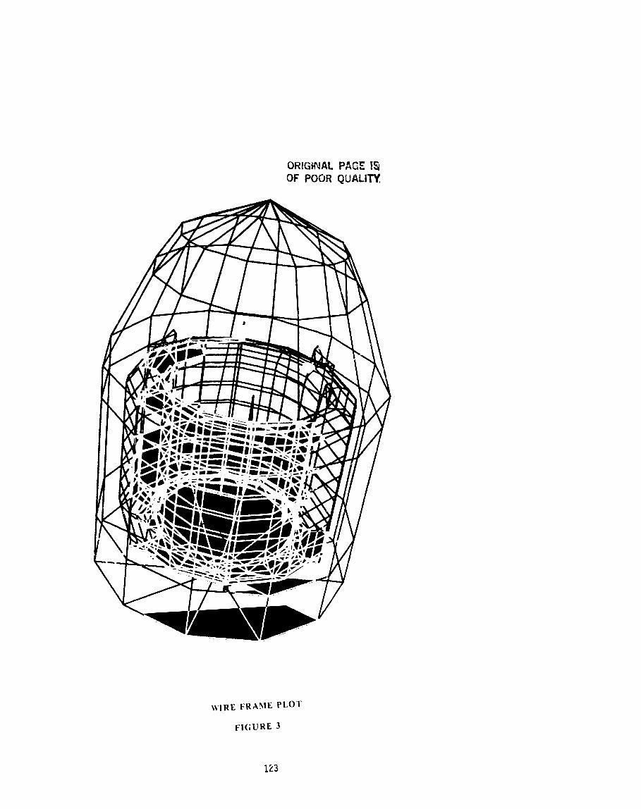
Clearly the most important feature of NPLOT is its ability to create hidden lir,: and haloed line views of mathzmatical models both quickly and accurately. The hidden line algorithm generates views of models with all hidden lines removed, figure 1 . The haloed line algorithm displays vie\.s with a f t lines broken i r an effort t r show depth while keeping the entir mods1 visible, figure 2 . A discussion of these algorithms follows in the next section. NPLOT, of course, also can plot a normal all lines visible view of a model usually referred to as a wire frame view, figure 3.

Another important feature of NPLOT that allows it to perform post processing is its ability to plot deformed shapes, figure 4. NPLOT reads the displacements from a NAS *'RAN F06 file. It can read either static displacements or eigenvectors.

All subcases or mode shapes can be read in a t once. The displacements arc written into a unformatted scratch file where they are available for rapid access when the user wishes to display a deformed shape. It is then a simple matter to enable the deformed shape, change subcases or mode shapes and change the scale factor for subseq~ent plcts.

NPLOT allows the user to specify elemeo t filters which select specific elements for plotting. Elements can be selected based upon t t .r type, property, and ID. Elements can aiso be selected 5~ a model segment. This is a:complished by inserting special segment delimiters in the bulk data deck and then specifying the delimiter label during the interactive session. Any or all of these filters c: I be activated a t the same time to allow a great deal of selectivity. The clemeats can then be labelled with their respective ID'S with a simple command once the plot i3 dicplayed on the screen, f igure 5.

NPLOT also allows the user con- siderable Leribility in specifying which grid points are to be labeled with their grid point ID'S. Specific grid point ID'S can be selscted and an eight character name tag can be associated with each grid poirrt. The name tag can be useful for distinzt identification. The user can aiso specify SPC sets, ASET and OMIT grid points to be labelled. These grid points will then be labelled with name tags indicating thc degrees of freedom involved, figure 6.

NPLOT allows the standard display operations such as rot-tion and perspective. l* also allows different view planes io be selected. These are X-Y, Y-Z and X-Z viewing planes. A ;.oom functior. is also allowed on terminals with a locator such as a grapllics cursor, tablet, light pen or joy

stick. The center of the area desired for zooming is selected with the locator and then a numeri: key is pressed to indicate the zoorning scale factcrr. Another display feature available is the Z-axis cut option which allows the user to cut away 3 percentage of the fore part of the model. figure 7. This is xseful because i t can reveal detail on the inside of a nodel.

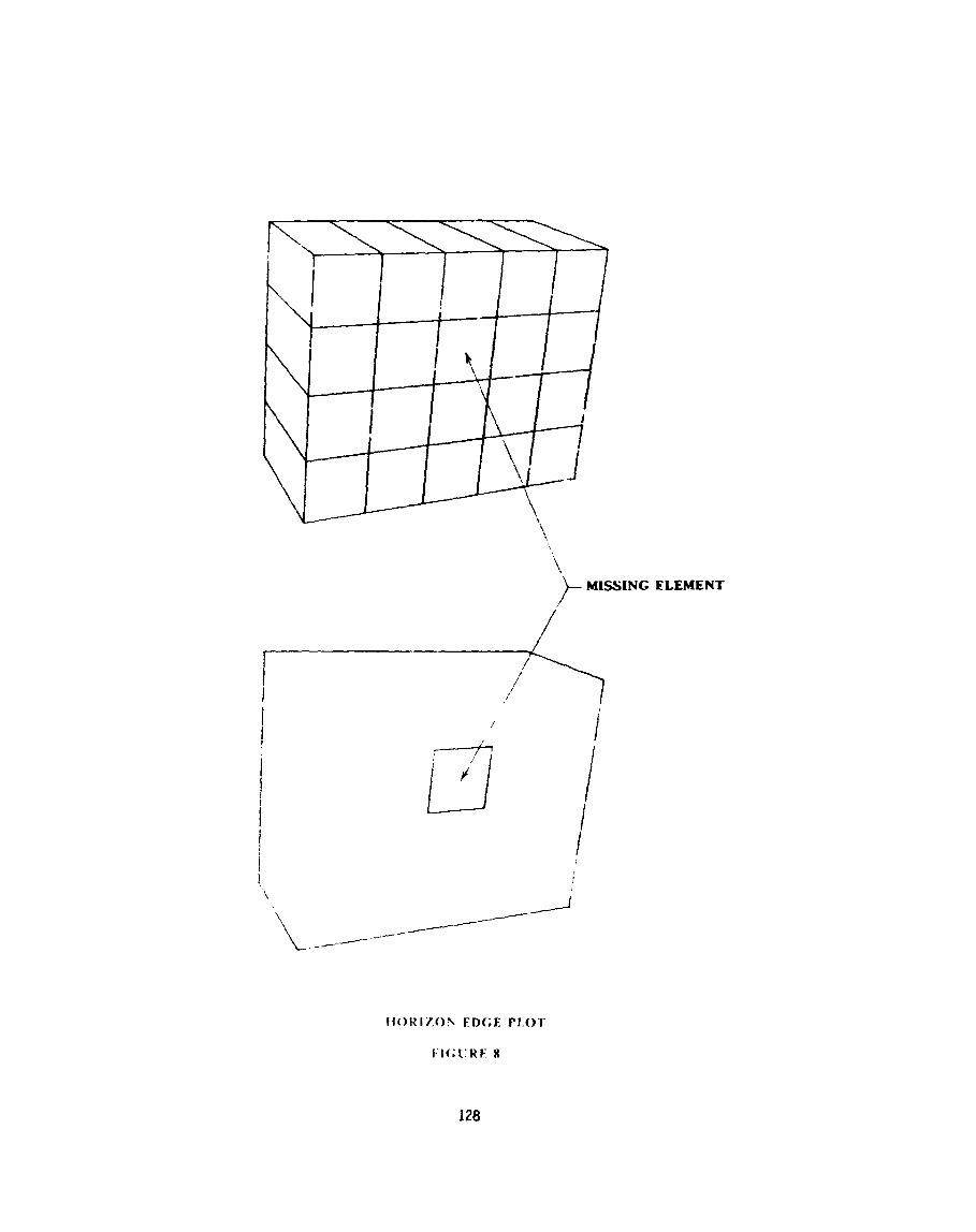
The calculation of the model's horizon edges ( edges where visibilty can change ) is normally used just to speed up the hidden line computation. Howcver, missing elements can lie cieariy located 10; qos t models by just plotting the horizon edges. NPLOT lets the user toaglc the display set from all edges to just the horizon edges. Illustrnted in figure 8 is a wire frame plot of t i e horizon edges for a model with a missing eiemcnt.

Another feature that aids the user is the plo! fi!e generator. Before beginning a plot the user can toggle on the plot file generator which will write all subsequent plot labels and screen vectors into a plot file until the toggle is turncd off again. This plot fiie can then be read by other p r ~ g r a m s such a pen plctter program. The HP7580A pen plotter is used by GSFC's Mechanical Engineering Branch when larger and more precise plots are desired.

User Inter faL-e:

NPLOT'S user interface is in- tended :o make NPLOT easy and quick to use. i t is also intended to allow frequent users to become eff iciel t a t using the program. Frequent use will enable users to takc short cuts once thcy are familiar with the instruction ,et. This aim is accomplished by using a combination of menu and command driven user interface with available help menus for detailed information

concerning ezch command. NPLOT is Within each s f these menus sre controlled via commands from two commands that invoke sub-menus. The mlin menus. The basic command/nenu input menu is used for selecting structure is: elemtnt sets, element labels, grid lateis

and deformation sets. The plot menu is used to select the display operations and then to execute the plot option desired. Once the plot is on the screen the interface becomes commaiid driven. The same commands that were available from the preceding menus are now available for immediate execution. This enables the frequent user to avoid returning to the men3 every time he wisna to manipulate the display or execute a command.

I I I <---- INPUT bUfLK DATA DECK

I I +< ----. .----- --+

I I I I I +---- > ELEMENT SELECTION MENU

I I +----> LOAD DEFORMATIONS MENU

COMMAND MENU STRUCTURE

HIDDEN LINE / HALOED LINE ALG0WITHI.S

Hidden Line:

The development of a new hidden line algorithm was not taken lightly. Tetht iques to perform hidden line plotting have been much discussed beginning with the advent of computer graphics in the early 1960's arid continuing into the present err. Given the bulk of this prior wo;k [3-11,. why develop a new method? The answer is that t b s e prior methods, as of 1980, appeared to lack the speed necessary for ef;:ctive interactive use, lack features necessary to plot NASTKAN models, or the referenced papers provided i~su f f i c i en t implementation details. Except for the Watkins technique [ I 11, coded algorithms were not available. Experience iu using the Yatkins technique had shown it to be not acceptab!~ for hidden iice p lo t t~ng of NASTXAX models. Refsrences 12 through 16 werr ~ubl i shed efter our algarithm had L e n s~bstant ial iy completed.

Several different variations of the s lme basic hidden line method havr k e n sequentially developed by G. Jones in the course of this effort. To kecp track of the different versions, they were assigned names JONES/A through JONES/E. JONES/D was u s ~ d in the first productio2 version of NPLOT and was described in reference 17. The fastest and most rrcent version of the hidden iine algorithm, JONES/E, is incorporated into the current version of NPLOT. The basic flow for JONF.S/E is as follows:

1. INPUT: The main inputs to JONES/E from NPLOT are the globai edge list, giobal surface list, edge/surface adjacency table and

grid point table. It should be ndted that NPLOT operates to produce nonredundant global edge and surface lists. The global surface list uses r four node flat surface representation; NPLOT processes triangles through 20 node solid elements to this sur'ace data format.

2. PREPARATION: The edge and surface lists are 2rocessed to produce arrays for edge and surface data. For example, the minimum/naximum X, Y, and Z values for e?ch edge and surface are computed. The horizon edges of the object for the viewing trarlsformarion are computed. Fpatial sorting of the edge and surface data is performed. Illustrated in figure 9 is a simplistic view cf thz spatial sort cells used by JONES/E. Based on the complexitj- cf the model, N x N mesh X-Y sort cel:s are iiaposed ori the model s a d lists of pointers to horizon edge data and surface data are generated for eacii cell \-ia bucket sorting. Different mesh densities arc csed for edge and s u r f ~ c e sorting. The mesh density used for the horizon edge sort is based on the total number of edges in the model. The mesh density for surface sorting is based on the number of surfaces In t5e model. The functional relationship between these measures of model complexity and mesh densities are set heuristically by varying the mesh density and observing the resulting performance for a number of models. JONESjE currently uses mesh definitions derived for JONES/D and so may not be optimum. After the cell lists are created, they are dr1:ih sorted based on the depth of the horizon edge or surface.

3. EDGE VISIBILITY: The global edgc list is precessed in two passes. On the first pass only the horizon edges are processed and the remaining edges are processed on the second pass. In either case the silbsequcnt loop operations arc the same. The edge cell coordinates for the cdgc arc dctermincd via a look-up table. The cdge cells associated with the cdgc are binary searched to find the depth to limit the search for horizon edges that intersect wrth the cdge. !ts inter- sections with all horizon edges, that have not been found to bc invisible by a prior calculatiov, arc determined. The edge is broken into segments s i n g its end points and the points of intersectian. Each segment is either ail visible or all invisibl:. Thr 3id-point of each se;mcnt is computed and checked against the appropriate cell surface list to ascertain visibility. This requires computing the surface cell coordinates fc r the mid-point and thcrl performing a binar) search to find the depth in the surface cell list to l i m ~ t the search for obsc~r ing surfaces. Containment and depth computations arc then performed to ascertain mid-point visibility, and hence, segment visibility.

This algorithm was tailored to support the plotting of NASTRAN models, therefore in the current implementation:

1. A line penetrating a surface usually results in a visible plot error. This is desirable for NASTRAN plotting since this usually indicates a modelling error.

2. Grid pcints a r t required where e l e m ~ ~ t s meet. This is normally :he case in NASTRAN models.

3. Surfaces must bc ~ ' a n a r Cor accurate plotting. Thic is true for commonly used NASTRAN clc- ments.

In operation, the algorithn; is remarkably fast for plotting NASTRAN mdels . There are two chief reasons for :his speed. The first being the efficiency of the spatial sort and the horizon cdge technique in reducing the number of edgc to edgc compares in computing the required line intersections. Thc second being the effectiveness of the spatial sorts in reducing mid-point to surfacc compares in computing edge scgment visibility.

i h e spatial sort func t ims as a diviac and conquer technique; this is facilitated by the fact that in general NASTRAN models have fairly uniform topologica1 granularity and the relative granule size decreases as model size increases. Thus. the spatial sort serves to linearize th= operation of the algorithm. It is worth noting that Writtram 1141 in a article published concurrently with the development of NPLOT riszd a horizontal strip form 3f spatial sort to achieve a high speed hidden line algor- ithm. The form of the spatial sort in JONES/E, and in the prior JONES/D. algorithm ia somewhat different from Whittrrm's in that the spatial cells are boxes not strips and the fact that in JONES/€ ( a1.d JONES/D ) the hidden line de~ermiqation does not make use or tt.e concept of an active edge list or an active polygon list to reduce the computations.

The main difference between the current JONES/E algorithm and the prior JONES/D is the addition of the horizon edgc method to the algorithm. A horizon edge is any model edge across which visibility can change. The concept of using horizon edges in hidden line computaiion was noted by Appel [I%] and nrcrc rzcently used by

Hornung [16] to generate a very high speed hidden linc algorithm for closed single surface objects. In JONESiE, horizon cdges arc computed 2nd used to drastically reduce the number of edgc ccmpare cs ra t ions . On a per cell basis, the reduction in operations is from the order o; total edges squared to horizon edges times total edges. The net effect of using horizon edges was to speed up the a:ljorithm by about 50 percent.

The a u i h o r ~ make no claim to havc "solved the hidden line problem'. Contrprv to vdha- some havc claimed, it appear< Inat ns existing algorithm is effei:;ivc; for @he full 5p:ctrum of coramor ior;clogi=o, for example curbed suifaccs. Inaacquate research and a la:-k of understanding of the problem are usually evident when such claims are put forth. JONES/€ was simply designed to prccess NASTRAN models or other similar topologies iri an efficient manner.

Haloed Line:

The use of haloed linc plotting wzs lirst discussed by Appe; [5 ] . In haloed line plotting, the a f t edges are broken whcrc they intersect with more forward edges; this produces a well de- fined depth effect for the viewer, figure 2. The initial haloed line code for NPLOT was written by T. Carnahan, GSFC, based on the tech- niqges defined by .Appel [5 ] . The haloed line algorithm in the current version of NPLOT has been recoded by one of the authors ( G. Jones ) to incorporate the same spatial sort techniques as in the JONES,'E hidden line algorithm and thereby increase its speed of operation.

Haloed line computation re7uires much m9re line intersection calculation than hidden line plotting thereby

increasing the cpu time. Whereas hiddzn line plotting effectively truncates the total edgc list. haloed !inc p l ~ t t i n g operates to increase the total edgc list by sp!itt;ng up edges ifito sebcrat wegents Thus, haloed line plottin$ generates more terminal i /O thao wire frame or hiddcn line plotting. For these reasons, haloed line plotting should be s l ~ a c r tnan the other plot types.

In haloed line plotting the SPLOT user can specify the size of the gap sa as to produce different effects. Haloed line plotting can be very effective in certain situations:

1. For models with few ~ u r f a c c elements but many iine elements, CBAR's and CROD's, haloed linc plotting is very effective a t show- ing depth information. Hidden tine plotting is ineffective for this type of mitdel.

2. When the user wants to peer inside a model but retzin depth cues. haloed line plotticg i s dr! efiective technique. This is similar to allowing transparency in hidden surface plotting on taster devices.

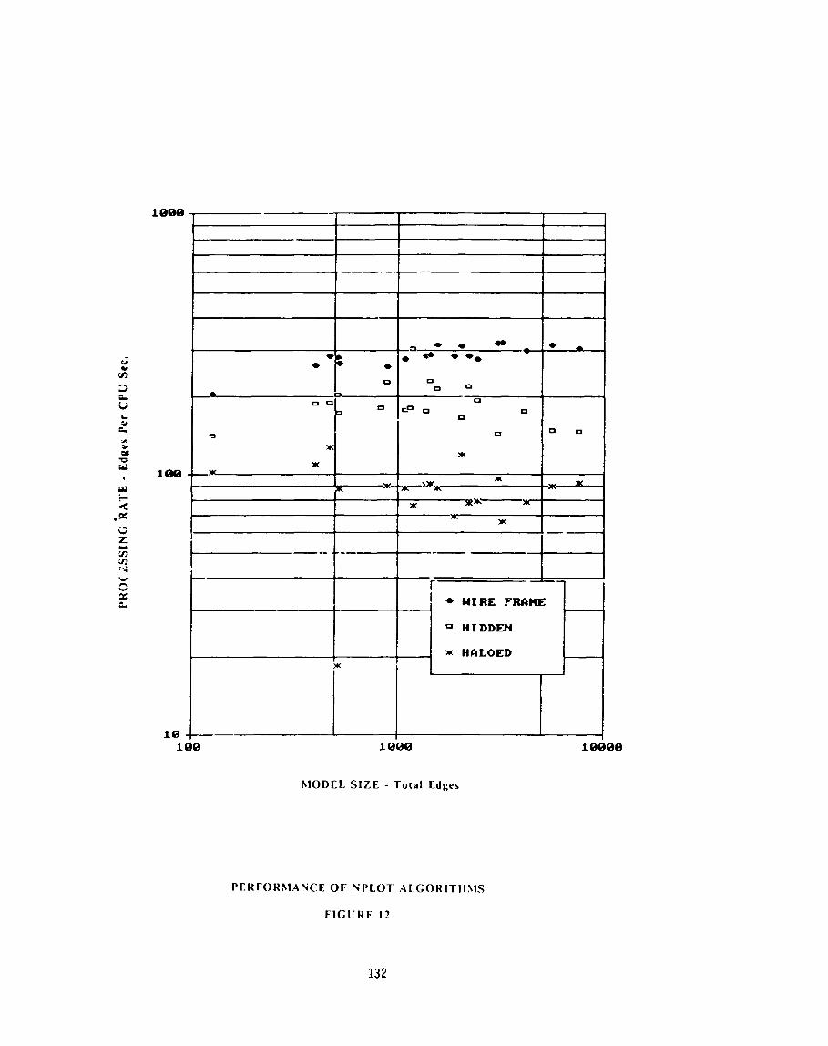
The basic performance of the three plots type in NPLOT were assessed by measuring their performance with a collection of 20 NASTRAN modele. The model sizes ranged from 55 grids/126 edges167 surfaces up to 3730 grids/7547 edges /3626 surfaces. Wire frame and hiddcn line plots or the largest riicdel are shown in figures 10 and 11. The performance of the algorithms werc measured in terms of a processing rate expressed in terms of edges per cpu second. The cpu times were aeasured on a normally loaded V A X l li780

computer and included the time to perform any preparatory work, execute the plot function module ( wire frame, haloed. hidden ), run the PLOT10 module, and perform the 110 to paint the object on the screen.

Shown in figure !2 is a graph of the measured performance of the three algorithms. All three algorithms show fairly linear performance f c r the range of modcls used in the tests. Wire frame plotting yielded an average ratc of about 300 edges per cpu sccond, hiddcn line plotting was somewhat slower a t about 150 edges per cpu second and haloed linc plotting was t5c slowest a t around 100 edges per cpu second. Wall clock response time for hiddcn line plotting was about the same as that for wire frame plottine. This -.?as due to the fact that hidden line plotting involves less terminal I/O than wire frame plotting. Haloed linc plotting was the slowest but this was expected. Even so, haloed line plotting was sufficiently fast to meet the demands of the interactive user. Haloed line plotting is the preferred ploi type 'or modclz with few surfaces and many line elements.

Thc net effect of the v ~ r i 3 u s optimizing techniques employcd In the hidden line algorithms can be seen from our experience in plotting onc of the test models. The first - cut hidden line aigorithm was a basic brute force line intersection technique with little code optimization; its processing rate for the test model was about 2.5 eJges per cpu second. A subsequerrt verslon with more code optimization and a few sinplc short cuts worked .it a rate of about 18 edges per cpu cecond. The JONES/D algorithm, which used the X-Y spatial sort, performed a t a rate of about 100 edges per cpu second. The IONES/E algorithm in the current version of NPLOT uses the X-Y spatial sort together with the horizon edge

technique. and achieves a precessing rate of about 175 edges per cpu second for this particular model. Thus in th i j instance JONES/E performs about 70 times quicker than a brute force method.

How fast can an optimum hidden linc algorithm run? A reasonable bounding upper limit might be the speed for wire frame plotting. For the particular hardware / software used a t our computer facility ( VAX 11/780, FORTRAN 77, Tektronix terminals using 9600 baud ) the wire frame process ratc was a b u t 300 edges per sccond, thereby implying that no hidden line algorithm could run more than twice as fast as JONES/E for this particular computing environment.

The Watkins hidden !ine/surface method [I I] and Hedglcy's algorithm were compare0 to the JCNES/E algorithm via comparative testing. The MOVIE program uses the Waikins method for hidden line and hiddtn surface computation. A VAX imple- mentation of MOVIE was used f ~ r this ;tudy. The MOVIE implementation of Watkins does not support line element types so an all surface model was used to make the comparison. The test model consisted of 857 surfaces and 1242 edges. The cpu time for just the hidden line generation ir. MOVIE was 41.5 seconds; the corresponding time for NPLOT was 6.9 cpu seconds. The SKETCH hidden line routine develcped by Hedgley [I31 was obtained and converted to the VAX 11/780 c o m o ~ er. The routine as delivered w;s limitcd to about 250 polygons; therefore, a relatively small model was used for testing, 183 surfaces/324 edges. The cpu time for SKETCH was 19.3 cpu seconds and the time for the JONESIE algorithm in NPLOT was 1.9 cpu seconds. The level of performance f ~ r SKETCH, about 9 polygons per cpu second, s c m s cmsistent with the data

presented by Hedgley [13& In ref- erence 13 the procc,sing rate for SKETCH on a CDC 6500 computer, which is about the same speed as a VAX 111780, was given as about 10 polygons per cpu second.

CONCLUDING REMARKS

The NPLOT computer graphics program has been shown to be an effective tool for the interactive display of NASTRAN finite element models. It offers a variety of na t c of the a r t t w l s to aid the analyst. It is easy to use and provides an on line help facility for the inexperienced user. N P L 3 T s very fast hidden line and haloed line algorithms are unique and effective graphics tools for the analyst. Analysts using NPLOT usually prefc: hidden line or haloed line plots in place of wire frame plots due to the more realistic model display. Current activity is focused on increasing the post-processing functionality of NPLOT.

REFERENCES

1. Walker, W., and Vos, R., IAC Excut- ive Summary, NASA CR- 175 196, May 1984.

2. Vos, R.G., Beste, D.L., and Gregg, J., IAC User Manual, NASA CR-175390, July 1984.

3. Newman, W.M, and Sproull, R.F., Principles o j Interactiva Computer Graphics, McGrsw-Hill Co., 1979.

4. Bareau, H., "Convenient Represent- ation Method For Spatial Finite Element Structures", Computers & Structures, 19(5), October 1979, pp. 815-819.

5. Appel, A., Rohlf. F.J.. and Stein, AJ, T h e Haloed Linc Effect for Hidden Line Elimination', Computer Graphics, 13(3), August 1979, pp. 151-157.

6. Franklin, W.R., "A Linear Time Exact Hidden Surface Algorithm", Computer Graphics, 14(3), August 1980, pp. 1 17-123.

7. Giloi, W.K., Interactive Computer Graphics. Data Structures, Algor- i t h m . Languages, Prentice-Hall Inc., 1978.

8. Griffiths, J.G., "A Surface Display Algorithm". Computer Aided Design, 10(1), January 1978, pp. 65-73

9. Griffiths, J.G., 'A Bibliography of Hidden-Line and Hidden-Surface ~:gorithms",Computer Aided Design, 1 O(3 r, May 1978, pp. 203-206.

10. Griffiths, J.G., "Tape-Oriented Hid- den Line Algorithm", Comquter Aided Design, 13(1), January 1981, pp. 19-26.

11. Watkins, G.S., A Real Time I'isible Surrare Algorithm, University of Utah, UTEC-CSc-70-101, June 1970.

12. Emery, A.F., VIEW, University Of Washington, Department of Mechanical Engineering, 1982.

13. Hedgley, D.R., Jr., A General Solution to the Hidden Line Problem, NASA RP-1085, March 1982.

14. Writtram, M, "Hidden-Line Algor- ithm for Scenes of High Complex- ity", Computer Aided Design, 13(4), July 1981, pp. 187-192.

15. Janssen, T.L., "A Simple Efficient Hidden Line Algorithm", computer^ & Structures, 17(4), 1983, pp. 563-57 1.

IdHornung, C., 'An Approach T o A Calculation-Minimized Hidden Line Algorithm', Computers & Graphics, 6(3), 1982, pp. 121-i26.

17. Jones, G.K., A Fast .Yidden Line Algorithm For Plotting Finite Element Models, NASA TM-8398 1. August 1982.

18. Appel, A., 'The Notion o f Quant- itative Invisibility and ;he Machine Rendering of Solids", Proc. AChf National Conference, 1967, pp. 387-393.

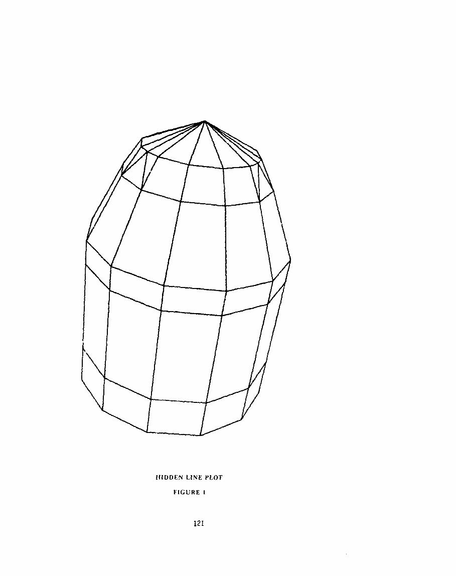
I1IDDEN L I N E PLOT

FIGURE 1

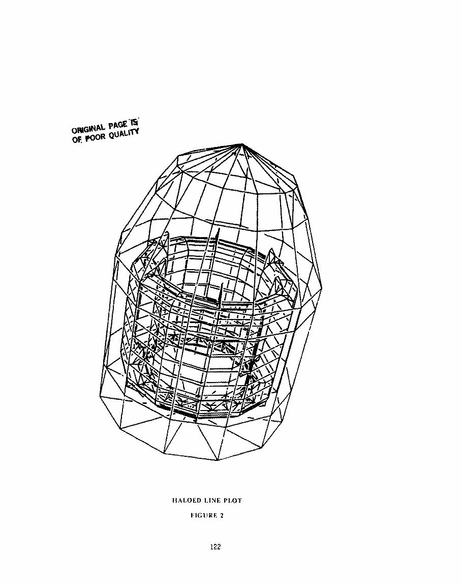
I jALOED L I N E PLOT

F I G U R E 2

ORlGWVAL PACE 14 OF POOR QUALITY

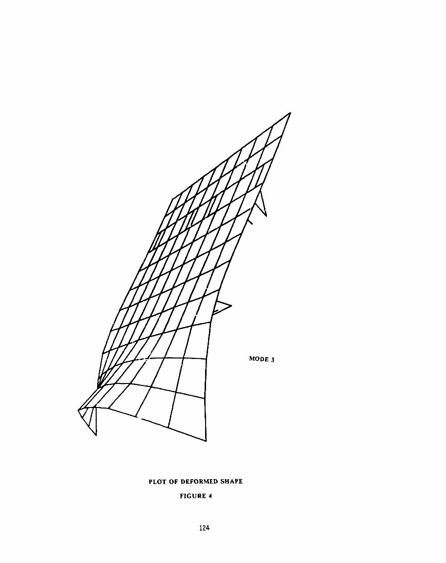
PLOT OF DEFORMED SHAPE

FIGURE 4

PLOT WITH ELEMENTS L.ABELI.ED

F I G U R E S

PLOT WI'fH GRIDS LABELLED AND TAGGED

FIGURE 6

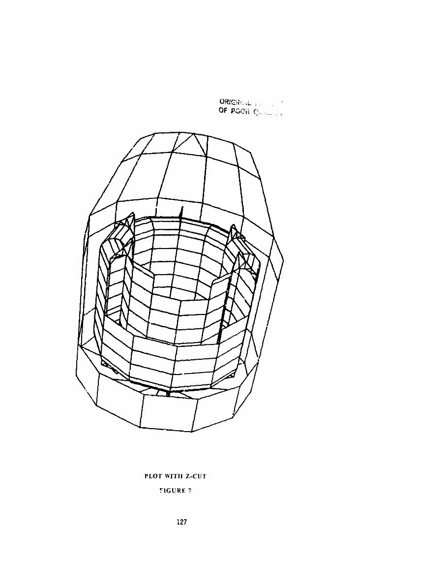
PLOT \VITJi Z-CUT

FIGURE 7

U I S I N C ELEMENT

I ---+ I

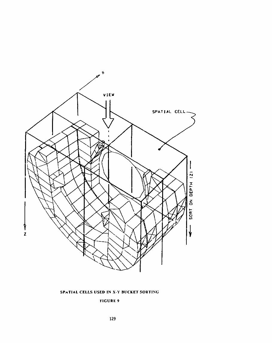
SPATIAL CELLS USED IN X-Y BUCKET SORTING

FIGURE 9

LARGE TEST hlODEL - \VIRE F R A h l E PIJOT

FIGURE 10

I,.AHCE TES-T hlODEL - I I I D D E N L I N E 1'1.0-i'

FICC:RE 1 1

-

lee

* WIRE FRRME HIDDEN

x HALOED

18 188 1008

hlODEL S I Z E - Total Edges