NOZZLE DESIGN FOR A SMALL, LOW-SPEED, CLOSED-RETURN

WIND TUNNEL

By

Jeremy S. Martin

A thesis submitted in partial fulfillment of the requirements for the degree of

Bachelor of Science

Houghton College

May 2019

Signature of Author…………………………………………….…………………………………. Department of Physics

May 3, 2019 ……………………………………………………………………………………………………………...

Dr. Kurt Aikens Assistant Professor of Physics

Research Supervisor ……………………………………………………………………………………………………………...

Dr. Brandon Hoffman Professor of Physics

2

NOZZLE DESIGN FOR A SMALL, LOW-SPEED, CLOSED-RETURN WIND TUNNEL

By

Jeremy S. Martin

Submitted to the Department of Physics on May 3, 2019 in partial fulfillment of the

requirement for the degree of Bachelor of Science

Abstract

Wind tunnels are used to characterize objects aerodynamically (e.g., measure lift and drag

as a function of air velocity). They are critical in the design process of many products,

including cars and planes. At Houghton College, a wind tunnel is currently being designed

and built. One of the most difficult components of a wind tunnel to design is the nozzle,

which contracts the air to produce a high-speed flow immediately upstream of the test

object. This is difficult because the nozzle must be designed to produce a uniform flow at

the exit to get an accurate representation of how air flows over the object. Furthermore, to

improve flow uniformity and to increase efficiency, boundary layer separation is to be

avoided inside of the nozzle. For the present wind tunnel, several commonly used nozzle

designs were tested in order to determine which best fulfills the requirements above.

These nozzle designs were tested using viscous, turbulent air flow simulations in ANSYS

Fluent. Results and conclusions will be presented and future work highlighted.

Thesis Supervisor: Dr. Kurt Aikens Title: Assistant Professor of Physics

3

TABLE OF CONTENTS

Chapter 1 — Introduction ........................................................................................................... 5

1.1. Motivation and Background ...................................................................................... 5

1.1.1. Introduction ......................................................................................................................... 5

1.1.2. History .................................................................................................................................... 6

1.1.3. Types of Wind Tunnels .................................................................................................... 8

1.2. Nozzle Design ................................................................................................................ 11

1.3. Objective ......................................................................................................................... 12

Chapter 2 — Theory ...................................................................................................................... 14

2.1. Governing Equations .................................................................................................. 14

2.2. Computational Methodology ................................................................................... 19

2.3. Flow Phenomena ......................................................................................................... 21

2.3.1. Laminar vs. Turbulent Flow ........................................................................................ 21

2.3.2. Boundary Layer ............................................................................................................... 22

2.3.3. Separation .......................................................................................................................... 23

Chapter 3 — Numerical Experiments ................................................................................... 26

Chapter 4 — Results and Analysis.......................................................................................... 32

Chapter 5 — Conclusion ............................................................................................................ 36

4

TABLE OF FIGURES

Figure 1. Diagram of forces acting on an object in a wind tunnel ............................................... 5

Figure 2. Diagram of a whirling arm apparatus ................................................................................. 7

Figure 3. Diagram of wind tunnel built at Gottingen, Germany in 1916 .................................. 9

Figure 4. Diagram of an open circuit wind tunnel ............................................................................. 9

Figure 5. Diagram of a closed return wind tunnel ......................................................................... 10

Figure 6. Diagram of wind tunnel at NASA Ames ........................................................................... 10

Figure 7. Diagram of a flow being contracted .................................................................................. 19

Figure 8. Two-dimensional, structured mesh .................................................................................. 21

Figure 9. Smoke visualization of a laminar flow becoming turbulent when it interacts with a stationary object. ........................................................................................................................... 22

Figure 10. Image of laminar boundary-layer profile ..................................................................... 23

Figure 11. Image of separation of a laminar boundary layer .................................................... 24

Figure 12. Contour profiles of nozzles from the Bell and Mehta, Brassard, and Morel papers .............................................................................................................................................................. 27

Figure 13. The quarter-nozzle fluid geometry utilized for nozzle simulations .................. 28

Figure 14. Image of the fine mesh at the exit of the test section .............................................. 31

Figure 15. Image of planes created in the fluid geometry for simulation analysis ........... 31

Figure 16. Comparison of stagnation pressure loss for the three nozzles as a function of velocity ............................................................................................................................................................ 33

Figure 17. Comparison of flow uniformity in the test section for different nozzles when 2.24 m/s (5 mph) flow was produced in the test section ........................................................... 34

Figure 18. Comparison of ux,RMS/ūx for the three simulations performed on each of the three nozzles ................................................................................................................................................. 35

Figure 19. Picture of a wooden frame in the shape of the desired nozzle profile ............. 37

5

Chapter 1

INTRODUCTION

1.1. Motivation and Background

1.1.1. Introduction

A wind tunnel is an apparatus that drives uniform, high-speed air over an object. They are

frequently used for experimental tests when the aerodynamic properties of an object affect

its functionality. Tests in wind tunnels allow researchers to measure the forces and torques

that an object experiences in the x, y and z directions, as seen in Figure 1. Knowing these

forces and torques is useful for understanding object behavior and is critical in the

engineering design process. For example, the forces can be used to calculate the speed an

airplane needs to acquire for it to generate enough lift to fly. Wind tunnels can also be

utilized to assess the stability of the airplane, which is an important characteristic of an

aircraft. Wind tunnels are used for many applications outside of aviation, too. Often times,

the drag force acting on a ground vehicle (e.g., cars, trucks, trains) is measured in a wind

tunnel to determine efficiency of the vehicle [1]. Examples of more specialized scenarios

tested in wind tunnels include, tests of the effect of wind on buildings [2] and tests of

migratory birds [3]. These are just a few of the many applications wind tunnels have.

Figure 1. Diagram of forces acting on an object in a wind tunnel. Figure adapted from Ref. [4].

It is clear that wind tunnels have many purposes, however they are not the only way to

determine aerodynamic properties of objects. Computational fluid dynamics (CFD) is

6

commonly used to achieve results that traditionally could only be determined using a wind

tunnel. As technology has rapidly grown, the use of CFD has also greatly expanded. There

are many benefits to using CFD. It is often less expensive than experiments, for many

problems it is relatively fast, the entire flow field is estimated (e.g., velocity, pressure,

density), and complicated geometries and situations can easily be analyzed [5]. However,

one of the main problems with CFD is it can be inaccurate, which often stems from

limitations in computing power. CFD users often utilize physical assumptions and/or

models that are made based on our knowledge of fluid mechanics to reduce computational

costs. This causes CFD to be limited by our knowledge of fluid mechanics. Some common

areas where this causes problems is when simulating flows with turbulence and/or

separation, which are described in Sections 2.3.1 and 2.3.3 respectively [6]. In some cases,

these models are developed using experimental data from wind tunnels [5]. Also, to build

confidence in CFD software in certain areas, wind tunnels are used to verify the CFD

results. Therefore, while CFD is useful in many ways, wind tunnels are still needed for the

design process of many products and for the validation of CFD software.

1.1.2. History

The study of aeronautics started in the 1700s [7]. It was then that researchers became

interested in determining the forces, like lift and drag, acting on an object as it moves

through a fluid. Researchers tried several different ways of performing these

measurements. Initially, objects were placed where there was naturally a lot of wind and

this was used to produce high speed air over the object. However, it was soon realized that

natural sources of wind were too inconsistent and unpredictable to work very well.

Therefore, the solution was to create machines that would produce steady, uniform airflow

over the object.

One such device that was commonly used was the whirling arm shown in Figure 2. It was

first utilized by Benjamin Robins, an English mathematician, in the mid-1700s [7]. This

device had a long arm and the object was affixed to the end of it. The mass is allowed to fall

causing the cylinder that the rope is wrapped around to spin. This causes the arm and the

object at the end of it to also spin. This was a much more reliable way to produce a

7

repeatable airflow over an object. During the 19th century, many scientists used the

whirling arm to compile data on the aerodynamic properties of different shaped objects.

Generally, the properties the scientists were concerned with were the lift and drag forces

acting on the object. They used various techniques in order to determine these forces [8].

One of the simplest ways was to allow the object to reach a terminal velocity. The drag

force could be determined from the mass of the falling weight because the torque produced

by the weight is the same as the torque caused by the drag. Also, by attaching a balance

system to the vertical cylinder that the rope is wrapped around, the lift could be

determined from the amount of mass needed to keep the balance from rising as the arm

spun. However, it was discovered that these measurements were not always accurate. This

was in part due to the fact that, since the whirling arm spun in a circle, the object was

traveling in its own wake. Thus, the air that the object was travelling through was moving.

This made it difficult to measure the velocity of the object relative to the air. Therefore,

other ways to produce steady and uniform airflow over objects were explored.

Figure 2. Diagram of a whirling arm apparatus. Figure taken from Ref. [9].

In 1871, Frank H. Wenham built the first wind tunnel [7]. His wind tunnel was a 3.66 m

long 0.457 × 0.457 m box that had a fan blow air through it. He was a part of the

Aeronautical Society of Great Britain and through the use of the wind tunnel they made

substantial progress in measuring lift and drag forces on objects. Due to their

8

aforementioned problems, whirling arms became less common and wind tunnels replaced

them [8]. This led to the flourishing of the study of aerodynamics at the start of the 1900s.

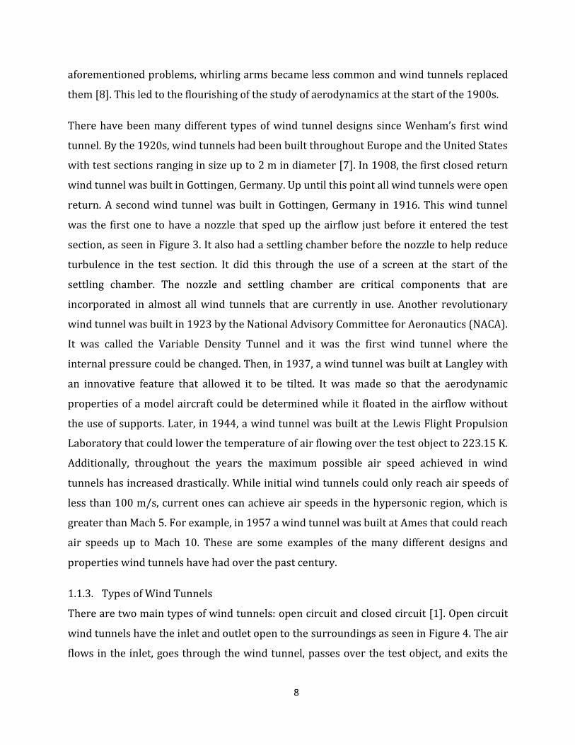
There have been many different types of wind tunnel designs since Wenham’s first wind

tunnel. By the 1920s, wind tunnels had been built throughout Europe and the United States

with test sections ranging in size up to 2 m in diameter [7]. In 1908, the first closed return

wind tunnel was built in Gottingen, Germany. Up until this point all wind tunnels were open

return. A second wind tunnel was built in Gottingen, Germany in 1916. This wind tunnel

was the first one to have a nozzle that sped up the airflow just before it entered the test

section, as seen in Figure 3. It also had a settling chamber before the nozzle to help reduce

turbulence in the test section. It did this through the use of a screen at the start of the

settling chamber. The nozzle and settling chamber are critical components that are

incorporated in almost all wind tunnels that are currently in use. Another revolutionary

wind tunnel was built in 1923 by the National Advisory Committee for Aeronautics (NACA).

It was called the Variable Density Tunnel and it was the first wind tunnel where the

internal pressure could be changed. Then, in 1937, a wind tunnel was built at Langley with

an innovative feature that allowed it to be tilted. It was made so that the aerodynamic

properties of a model aircraft could be determined while it floated in the airflow without

the use of supports. Later, in 1944, a wind tunnel was built at the Lewis Flight Propulsion

Laboratory that could lower the temperature of air flowing over the test object to 223.15 K.

Additionally, throughout the years the maximum possible air speed achieved in wind

tunnels has increased drastically. While initial wind tunnels could only reach air speeds of

less than 100 m/s, current ones can achieve air speeds in the hypersonic region, which is

greater than Mach 5. For example, in 1957 a wind tunnel was built at Ames that could reach

air speeds up to Mach 10. These are some examples of the many different designs and

properties wind tunnels have had over the past century.

1.1.3. Types of Wind Tunnels

There are two main types of wind tunnels: open circuit and closed circuit [1]. Open circuit

wind tunnels have the inlet and outlet open to the surroundings as seen in Figure 4. The air

flows in the inlet, goes through the wind tunnel, passes over the test object, and exits the

9

outlet. Closed circuit wind tunnels, on the other hand, are a loop that is closed off from the

surroundings as seen in Figure 5. The air does not enter or exit the wind tunnel but instead

continuously travels around the loop. Within these two types, wind tunnels can be a variety

of different shapes and sizes. An interesting and rare example which combines these two

types of wind tunnels is a NASA wind tunnel at Ames [7]. As can be seen in Figure 6, the

wall closure and exhaust louvers can either be open or closed allowing the wind tunnel to

function as either an open or closed return wind tunnel. It is also unique because it is large

enough to fit a full-sized aircraft in the test section.

Figure 3. Diagram of wind tunnel built at Gottingen, Germany in 1916. It was the first wind tunnel to have a nozzle before the test section. Figure taken from Ref. [7].

Figure 4. Diagram of an open circuit wind tunnel. Figure taken from Ref. [10].

10

Figure 5. Diagram of a closed return wind tunnel. Figure taken from Ref. [11].

Figure 6. Diagram of wind tunnel at NASA Ames. Figure taken from Ref. [7].

There are pros and cons for both types of wind tunnel designs. One of the main benefits of

the open return wind tunnel is that it usually costs less to build than closed return wind

11

tunnels because it takes less material and time to construct [1]. Also, sometimes smoke is

used in wind tunnels in order to visualize the flow of the air. This type of flow visualization

can cause problems in closed return wind tunnels because there is no way for the smoke to

escape the wind tunnel. However, open return wind tunnels do not have this problem. On

the other hand, there are multiple pros for closed return wind tunnels. First, they are not

affected by their surroundings like open return wind tunnels are. Closed return wind

tunnels are isolated from their environment, so the air flow inside of them can be highly

controlled. Conversely, open return wind tunnels are not isolated from their environment.

If located outside, the weather could have a large effect on the wind tunnel. Furthermore, if

the ends of the wind tunnel are located near walls or other objects, then extensive

screening is needed in order to produce uniform air flow in the wind tunnel. Another

benefit of closed return wind tunnels is they often require less energy to run than an open

return wind tunnel of the same size. Lastly, closed return wind tunnels are generally

quieter than open return wind tunnels. When deciding what type of wind tunnel to build,

these are the factors that are often considered along with available resources (e.g., money,

knowledge, time).

1.2. Nozzle Design

There have been multiple studies done to determine the optimum nozzle for a wind tunnel.

One of these was performed by Morel, who used a numerical approach to determine the

optimal design of an axisymmetric nozzle whose contour profile was specified by two

matched curves [12]. An optimal design was one that avoided separation (discussed in

Section 2.3.3) and produced a uniform flow. In the study, several nozzle parameters were

varied to figure out how they affected these two criteria. From this, it was determined that

for larger contraction ratios and length to inlet height ratios, it is beneficial for the matched

point to be located farther downstream and that the optimal contour profile is made using

cubic curves.

Bell and Mehta also performed a study that used a numerical approach to determine the

optimal design for a nozzle [13]. However, they used a nozzle that had a rectangular cross-

section. From their results they concluded that a fifth order polynomial was the best

12

function for the contour profile out of the profiles that they tested. They also determined

that when considering the dimensions of the nozzle it is beneficial to have a length to inlet

height ratio of greater than 0.667 but less than 1.79. A ratio less than 0.667 leads to

potential separation at the inlet of the nozzle, and a ratio greater than 1.79 can cause

separation at the outlet due to the boundary layer increasing in size. The contraction ratio

of the nozzle should be in the range 6-10. For a fixed airspeed in the test section, wind

tunnels with smaller nozzle contraction ratios have greater flow velocities throughout the

rest of the tunnel than those with larger contraction ratios. Therefore, smaller contraction

ratios produce greater losses in energy across wind tunnel components than when larger

contraction ratios are utilized. For this reason it is advantageous to have a contraction ratio

greater than 6. However, ratios larger than 10 cause the biggest components (e.g., the

settling chamber) to be unnecessarily large.

Another study using a numerical approach to determine the optimal design of a nozzle with

a rectangular cross section was conducted by Su [14]. In this study, the two design criteria

that were considered were the pressure coefficient at the entrance of the nozzle and the

flow uniformity at the exit. From the analysis of these criteria it was determined that for

the contour profile the radius of curvature should be larger at the inlet than the outlet. At

the inlet, this causes the pressure coefficient to be lower which reduces the chance of

separation. At the outlet, a smaller radius of curvature helps the flow become axial and

provides a more uniform flow in the test section.

1.3. Objective

At Houghton College, students and a professor are collaborating to design and build a low-

speed, closed-return wind tunnel. In the past, a script was written to estimate various

properties of a closed-return wind tunnel given certain constraints (e.g., the size of the

room, maximum desired airspeed produced in the test section) and criteria [15]. Two

properties that the code estimated were the overall efficiency of the wind tunnel and

general dimensions of each component. Using these dimensions, simulations were

performed to determine the number of turning vanes needed in each corner in order to

reduce the energy loss across the corners [16]. All of this information was used to purchase

13

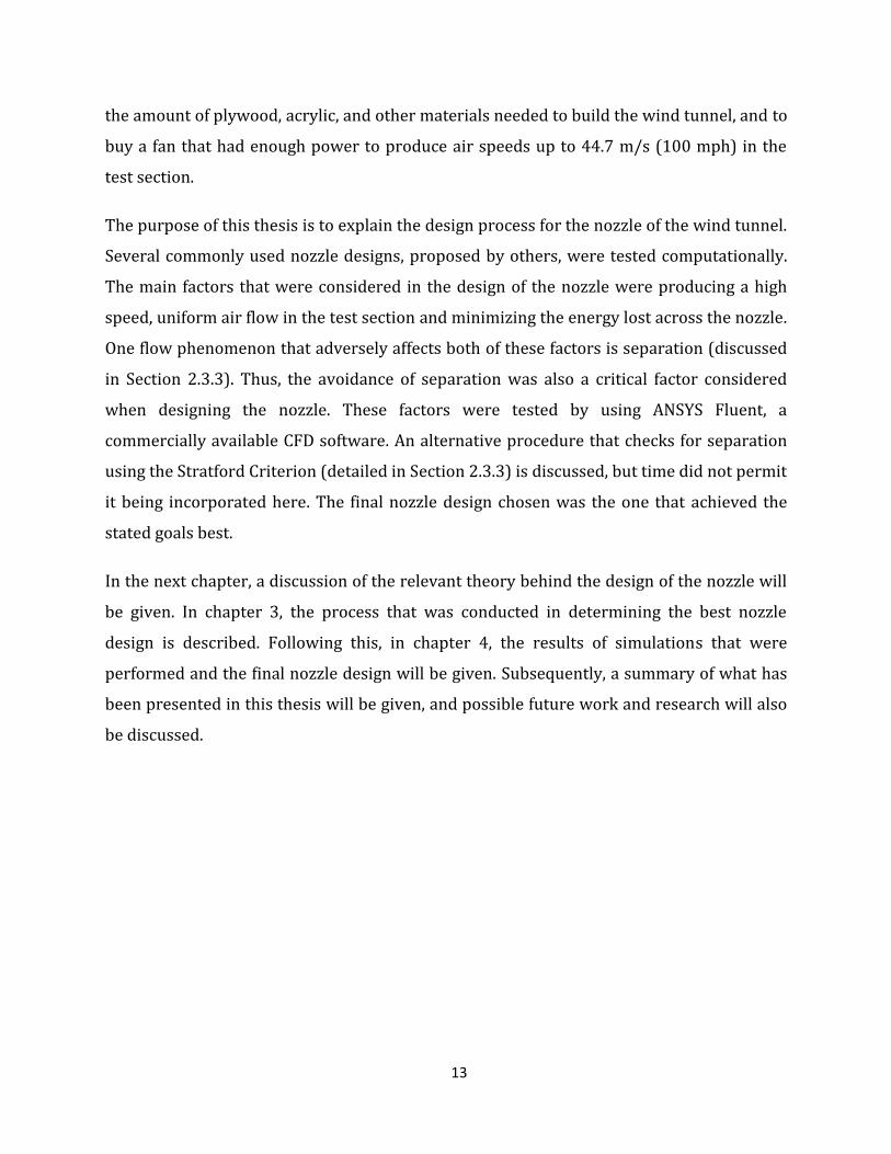
the amount of plywood, acrylic, and other materials needed to build the wind tunnel, and to

buy a fan that had enough power to produce air speeds up to 44.7 m/s (100 mph) in the

test section.

The purpose of this thesis is to explain the design process for the nozzle of the wind tunnel.

Several commonly used nozzle designs, proposed by others, were tested computationally.

The main factors that were considered in the design of the nozzle were producing a high

speed, uniform air flow in the test section and minimizing the energy lost across the nozzle.

One flow phenomenon that adversely affects both of these factors is separation (discussed

in Section 2.3.3). Thus, the avoidance of separation was also a critical factor considered

when designing the nozzle. These factors were tested by using ANSYS Fluent, a

commercially available CFD software. An alternative procedure that checks for separation

using the Stratford Criterion (detailed in Section 2.3.3) is discussed, but time did not permit

it being incorporated here. The final nozzle design chosen was the one that achieved the

stated goals best.

In the next chapter, a discussion of the relevant theory behind the design of the nozzle will

be given. In chapter 3, the process that was conducted in determining the best nozzle

design is described. Following this, in chapter 4, the results of simulations that were

performed and the final nozzle design will be given. Subsequently, a summary of what has

been presented in this thesis will be given, and possible future work and research will also

be discussed.

14

Chapter 2

THEORY

2.1. Governing Equations

The governing equations for fluid mechanics include a group of seven equations that

describe the motion of a fluid. The first of these equations is derived from the principle of

conservation of mass and it is called the continuity equation. It is given in tensor index

notation by the expression [17]

𝜕𝜌∗

𝜕𝑡∗+

𝜕

𝜕𝑥𝑖∗ (𝜌∗𝑢𝑖

∗) = 0, (1)

where * denotes a variable that has dimensions, t is time, ρ is the density, 𝑥𝑖 is the ith spatial

coordinate, and 𝑢𝑖 is the velocity in that direction. This equation can be

nondimensionalized by defining the nondimensional parameters

𝜌 =𝜌∗

𝜌0∗ , (2)

𝑡 =

𝑡∗

(𝑥0

∗

𝑢0∗)

, (3)

𝑥 =𝑥∗

𝑥0∗ , (4)

and

𝑢 =𝑢∗

𝑢0∗ , (5)

where 0 denotes a chosen reference value. By substituting the previous four equations into

Equation (1), the following expression is achieved

15

𝜕

𝜕 (𝑡 (𝑥0

∗

𝑢0∗))

(𝜌𝜌𝑜∗) +

𝜕

𝜕(𝑥𝑖𝑥0∗)

((𝜌𝜌0∗)(𝑢𝑖𝑢0

∗)) = 0. (6)

This can be simplified to

𝜕𝜌

𝜕𝑡+

𝜕

𝜕𝑥𝑖

(𝜌𝑢𝑖) = 0. (7)

This is the nondimensionalized form of the continuity equation.

The next three equations, the Navier-Stokes equations, are derived from Newton’s Second

Law. They are a statement of conservation of momentum and have the following form

when written in tensor index notation

𝜕

𝜕𝑡∗ (𝜌∗𝑢𝑗∗) +

𝜕

𝜕𝑥𝑘∗ (𝜌∗𝑢𝑗

∗𝑢𝑘∗ ) =

𝜕𝜎𝑖𝑗∗

𝜕𝑥𝑖∗ ,

(8)

where the components of the stress tensor, 𝜎𝑖𝑗, represent the stress acting on the fluid and

body forces are neglected. Notice that Equation (8) is three different equations, one for

each coordinate direction. The stress tensor is given by the expression

𝜎𝑖𝑗∗ = −𝑃∗𝛿𝑖𝑗 + 𝜇∗ [−

2

3𝛿𝑖𝑗 (

𝜕𝑢𝑘∗

𝜕𝑥𝑘∗) + (

𝜕𝑢𝑖∗

𝜕𝑥𝑗∗ +

𝜕𝑢𝑗∗

𝜕𝑥𝑖∗)] , (9)

where P is the pressure of the fluid and μ is the dynamic viscosity. To nondimensionalize

Equation (8), the nondimensional pressure is

𝑃 =𝑃∗

𝜌0∗𝑢0

∗2. (10)

Substituting Equations (2) through (5), (9), and (10) into Equation (8) and simplifying

gives

𝜕

𝜕𝑡(𝜌𝑢𝑗) +

𝜕

𝜕𝑥𝑘(𝜌𝑢𝑗𝑢𝑘) =

𝜕

𝜕𝑥𝑖(−𝑃𝛿𝑖𝑗) +

1

𝑅𝑒 𝜕

𝜕𝑥𝑖[−

2

3𝛿𝑖𝑗 (

𝜕𝑢𝑘

𝜕𝑥𝑘) + (

𝜕𝑢𝑖

𝜕𝑥𝑗+

𝜕𝑢𝑗

𝜕𝑥𝑖)], (11)

16

which is the nondimensional form of the momentum equations. In Equations (11) Re is the

Reynolds number and is given by the expression

𝑅𝑒 =𝜌0

∗𝑢0∗𝑥0

∗

𝜇∗. (12)

The Reynolds number for a fluid flow is significant because it gives the relative importance

of the viscous forces in the fluid. This means that flow scenarios that are geometrically

similar and have the same Reynolds number will produce the same nondimensional

results. This is a product of the governing equations being the same for both scenarios [18].

For incompressible flows, which is what the research presented in this thesis is concerned

about, there are only four variables: pressure and the three velocity components.

Therefore, only four equations, Equations (7) and (11), are needed to solve for the

properties of the flow. The following theoretical discussion, which is included for

completeness, is for flows that are compressible.

The fifth governing equation is derived from the principle of conservation of energy. First,

define the total energy per unit mass of the fluid as

𝑒𝑡∗ = 𝑒∗ +

1

2𝑢𝑗

∗𝑢𝑗∗, (13)

where e is the internal energy per unit mass and the second term is the kinetic energy per

unit mass. Then, the energy equation is given by the expression

𝜕

𝜕𝑡∗(𝜌∗𝑒𝑡

∗) +𝜕

𝜕𝑥𝑘∗ (𝜌∗𝑒𝑡

∗𝑢𝑘∗) =

𝜕

𝜕𝑥𝑖∗ (𝑢𝑗

∗𝜎𝑖𝑗∗ ) −

𝜕𝑞𝑗∗

𝜕𝑥𝑗∗, (14)

where q is the conductive heat flux.

So far, five equations have been defined with seven different variables in them. Therefore,

two more expressions are needed in order to have a system of seven equations with seven

variables. These last two expressions come from assuming the fluid is an ideal gas and that

the fluid’s specific heat is constant. The ideal gas law states that

17

𝑃∗ = 𝜌∗𝑅∗𝑇∗, (15)

where R is the ideal gas constant divided by the molar mass of the fluid and T is the

temperature. To nondimensionalize the ideal gas law, the nondimensional temperature is

written as

𝑇 =

𝑇∗

𝑇0∗,

(16)

and the definition of the Mach number is utilized, which is

𝑀 =

𝑢0∗

𝑎0∗ =

𝑢0∗

√𝛾𝑅∗𝑇0∗.

(17)

𝑎0∗ is the speed of sound in a fluid and 𝛾 is the ratio of specific heats. Equation (15) can be

nondimensionalized using Equations (2), (10), (16), and (17), which gives

𝑃 =

𝜌𝑇

𝛾𝑀2.

(18)

Lastly, by assuming that the fluid’s specific heat is constant, the internal energy of the fluid

can be written as

𝑒∗ = 𝐶𝑣∗𝑇∗, (19)

where Cv is the specific heat at constant volume. This is the last equation in the governing

equations for fully compressible flows: Equations (7), (11), (14), (18), and (19).

For a detailed study, it is necessary to use the unsimplified governing equations. However,

for certain situations it can be useful to simplify some of the governing equations by

making assumptions. For example, Bernoulli’s equation can be used to define the total

energy of the fluid. It is derived from the energy equation by assuming that the fluid flow is

inviscid (μ = 0), incompressible (ρ = constant), irrotational (�⃗� × �⃗� = 0), steady (partial

derivatives with respect to time are zero), and by neglecting body forces. It is given by [18]

𝑃 +1

2𝜌𝑢2 = 𝑃0 = constant, (20)

18

where P is the pressure, ρ is the density of the fluid, u is the magnitude of the fluid velocity,

and 𝑃0 is the stagnation pressure. The stagnation pressure can be thought of as the total

energy of the fluid per unit volume, the fluid pressure is a type of potential energy per unit

volume and the 1

2𝜌𝑢2 term is the kinetic energy of the fluid per unit volume. If the

assumptions made to derive Bernoulli’s equation are true, then the stagnation pressure will

be constant at every point in the fluid flow because energy is conserved. If the assumptions

are not valid however, the fluid loses energy as it travels from one point to another point

along its path. The amount of energy lost by the fluid is equal to the decrease in stagnation

pressure between the two points.

Another useful equation is the quasi-one-dimensional continuity equation. In order to

derive it, the divergence theorem is used to write the continuity equation, Equation (7), in

integral form as shown by the expression [18]

𝜕

𝜕𝑡∰𝜌𝑑𝒱

𝒱

+ ∯𝜌�⃗� ∙ 𝑑𝑆

𝑆

= 0, (21)

where 𝒱 is a given volume of fluid and S is the surface that defines the boundary of the

volume. Equation (21) can be simplified and applied to the general design of wind tunnels

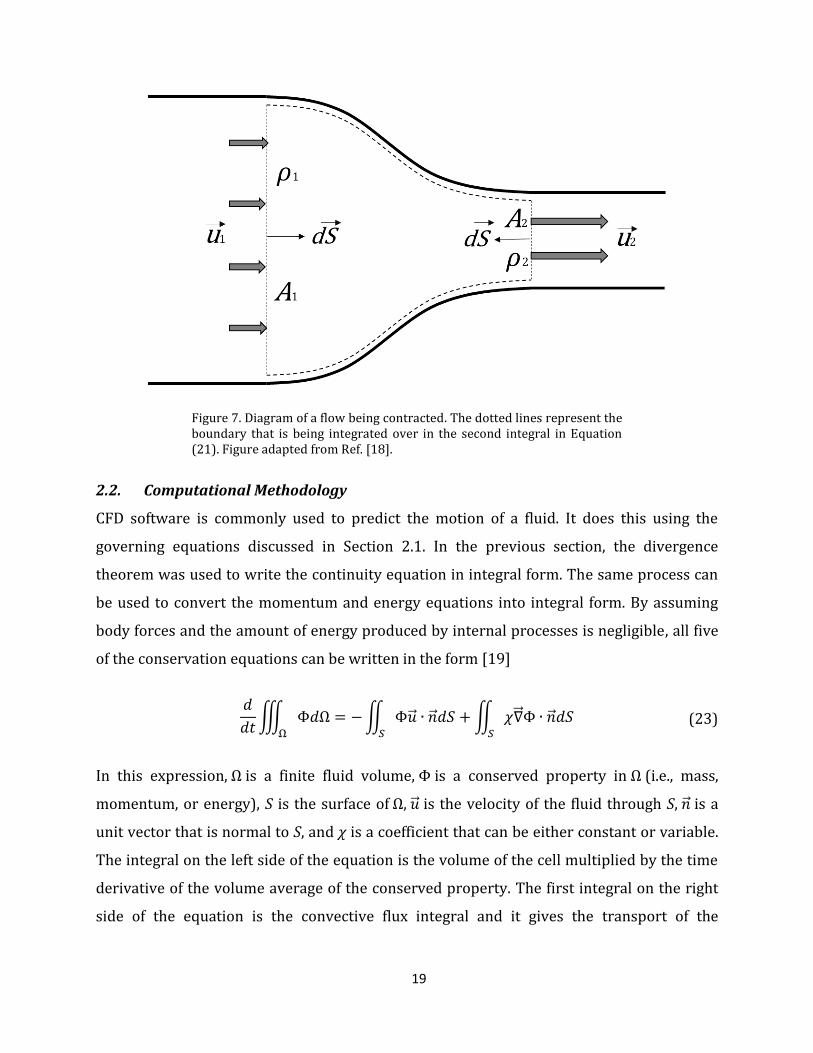
by making a few assumptions. Consider the situation depicted in Figure 7. By assuming the

flow is steady the first term in Equation (21) is zero. If it is assumed the boundary layer is

thin and the slope of the walls is small, then flow is parallel to 𝑑𝑆 throughout the cross-

sectional area but is perpendicular to 𝑑𝑆 along the walls. Therefore, if it is also assumed the

density and velocity are constant throughout the cross-sectional area the fluid is traveling

through, then the second integral can be integrated to give

𝜌1𝑢1𝐴1 = 𝜌2𝑢2𝐴2 = constant, (22)

where ρ is the density of the fluid, A is the cross-sectional area of the fluid, and u is the

velocity of the fluid. This equation is valid for both compressible and incompressible fluids

subject to the assumptions that have been made. In general terms, it is states that the mass

flow rate for all cross sectional areas is the same.

19

Figure 7. Diagram of a flow being contracted. The dotted lines represent the boundary that is being integrated over in the second integral in Equation (21). Figure adapted from Ref. [18].

2.2. Computational Methodology

CFD software is commonly used to predict the motion of a fluid. It does this using the

governing equations discussed in Section 2.1. In the previous section, the divergence

theorem was used to write the continuity equation in integral form. The same process can

be used to convert the momentum and energy equations into integral form. By assuming

body forces and the amount of energy produced by internal processes is negligible, all five

of the conservation equations can be written in the form [19]

𝑑

𝑑𝑡∭ Φ𝑑Ω = −∬ Φ�⃗� ∙ �⃗� 𝑑𝑆

𝑆

+ ∬ 𝜒∇⃗⃗ Φ ∙ �⃗� 𝑑𝑆𝑆Ω

(23)

In this expression, Ω is a finite fluid volume, Φ is a conserved property in Ω (i.e., mass,

momentum, or energy), S is the surface of Ω, �⃗� is the velocity of the fluid through S, �⃗� is a

unit vector that is normal to S, and 𝜒 is a coefficient that can be either constant or variable.

The integral on the left side of the equation is the volume of the cell multiplied by the time

derivative of the volume average of the conserved property. The first integral on the right

side of the equation is the convective flux integral and it gives the transport of the

20

conserved property through the surface. The third integral is the diffusive flux integral and

it gives the transport of the conserved property through the surface by diffusion.

CFD software determines the properties of the flow by estimating the solution to the right

side of Equation (23). In order to do this, the flowfield needs to be divided up into small

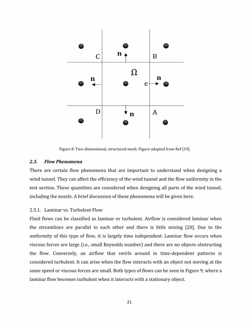
fluid volumes. This is done by creating a mesh. Figure 8 gives an example of a simple,

structured, two-dimensional mesh. The flow properties are estimated at the grid point

located at the center of each cell. Since this is a two-dimensional situation, the surface

integrals turn into line integrals. They can be approximated by

∫ 𝑓𝑑𝑆 = 𝑓�̅�𝐴𝐵 ≈ 𝑓𝑒𝑆𝐴𝐵,𝐴𝐵

(24)

where 𝑓 ̅is average value of the integrand of the line integral, 𝑆𝐴𝐵 is the length of the line,

and 𝑓𝑒 is the value of the integrand at the midpoint of the line. Since the flow properties are

not being directly solveed for at point e, interpolation from the grid points at the center of

the cells is used to estimate the value of 𝑓𝑒 . From Equation (24), for the two-dimensional

case, the two integrals on the right side of Equation (23) can be approximated as

∫ Φ�⃗� ∙ �⃗� dS = Φ�⃗� ∙ �⃗� ̅̅ ̅̅ ̅̅ ̅̅ 𝑆𝐴𝐵 ≈ (Φ�⃗� ∙ �⃗� )𝑒𝑆𝐴𝐵𝐴𝐵

(25)

and

∫ 𝜒∇⃗⃗ Φ ∙ �⃗� 𝑑𝑆𝐴𝐵

= χ∇⃗⃗ Φ ∙ �⃗� ̅̅ ̅̅ ̅̅ ̅̅ ̅̅ 𝑆𝐴𝐵 ≈ (χ∇⃗⃗ Φ ∙ �⃗� )𝒆𝑆𝐴𝐵. (26)

The same approximations can be made to determine the line integrals for BC, CD, and DA.

Note that the approximations utilized for these integrals improve with reduced cell sizes.

Then, these integrals can be summed to determine the right side of Equation (23). Similar

processes can be applied to three-dimensional and unstructured meshes. Once the right

side of Equation (23) is estimated, standard time integration procedures for ordinary

differential equations (e.g., Runge-Kutta methods) can be utilized to time-advance

estimates for Φ.

21

Figure 8. Two-dimensional, structured mesh. Figure adapted from Ref [19].

2.3. Flow Phenomena

There are certain flow phenomena that are important to understand when designing a

wind tunnel. They can affect the efficiency of the wind tunnel and the flow uniformity in the

test section. These quantities are considered when designing all parts of the wind tunnel,

including the nozzle. A brief discussion of these phenomena will be given here.

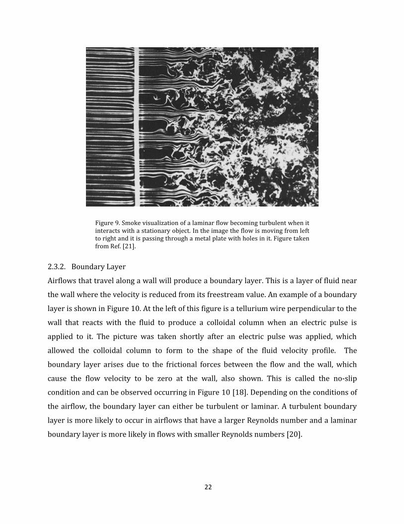
2.3.1. Laminar vs. Turbulent Flow

Fluid flows can be classified as laminar or turbulent. Airflow is considered laminar when

the streamlines are parallel to each other and there is little mixing [20]. Due to the

uniformity of this type of flow, it is largely time independent. Laminar flow occurs when

viscous forces are large (i.e., small Reynolds number) and there are no objects obstructing

the flow. Conversely, an airflow that swirls around in time-dependent patterns is

considered turbulent. It can arise when the flow interacts with an object not moving at the

same speed or viscous forces are small. Both types of flows can be seen in Figure 9, where a

laminar flow becomes turbulent when it interacts with a stationary object.

22

Figure 9. Smoke visualization of a laminar flow becoming turbulent when it interacts with a stationary object. In the image the flow is moving from left to right and it is passing through a metal plate with holes in it. Figure taken from Ref. [21].

2.3.2. Boundary Layer

Airflows that travel along a wall will produce a boundary layer. This is a layer of fluid near

the wall where the velocity is reduced from its freestream value. An example of a boundary

layer is shown in Figure 10. At the left of this figure is a tellurium wire perpendicular to the

wall that reacts with the fluid to produce a colloidal column when an electric pulse is

applied to it. The picture was taken shortly after an electric pulse was applied, which

allowed the colloidal column to form to the shape of the fluid velocity profile. The

boundary layer arises due to the frictional forces between the flow and the wall, which

cause the flow velocity to be zero at the wall, also shown. This is called the no-slip

condition and can be observed occurring in Figure 10 [18]. Depending on the conditions of

the airflow, the boundary layer can either be turbulent or laminar. A turbulent boundary

layer is more likely to occur in airflows that have a larger Reynolds number and a laminar

boundary layer is more likely in flows with smaller Reynolds numbers [20].

23

Figure 10. Image of laminar boundary-layer profile. The fluid is flowing from left to right. The black line at the left of the image is a tellurium wire that causes a colloidal column to form in the fluid when an electric pulse is applied to it. The curved dark line in the image is a colloidal column of particles that have been swept downstream by the motion of the fluid. Figure taken from Ref. [21].

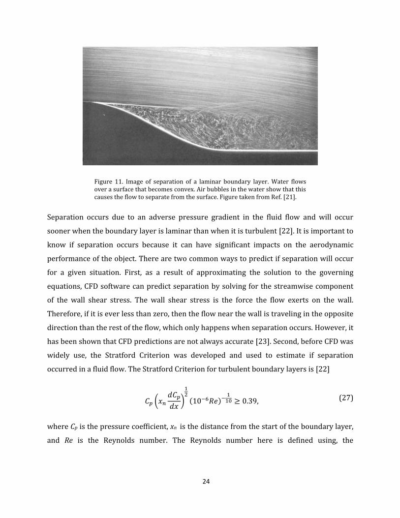
2.3.3. Separation

Separation is when the boundary layer of a flow leaves the surface of the object that it is

flowing over [18]. This creates a region between the surface and the main flow where the

fluid swirls in eddy currents and does not move in the same direction as the main flow. An

example of boundary layer separation is shown in Figure 11. In the figure, the streamlines

show the motion of the fluid. At the start, the parallel streamlines are right next to the wall,

but as the wall dips down a region is formed between the parallel streamlines and the wall.

This region is called the separation region.

24

Figure 11. Image of separation of a laminar boundary layer. Water flows over a surface that becomes convex. Air bubbles in the water show that this causes the flow to separate from the surface. Figure taken from Ref. [21].

Separation occurs due to an adverse pressure gradient in the fluid flow and will occur

sooner when the boundary layer is laminar than when it is turbulent [22]. It is important to

know if separation occurs because it can have significant impacts on the aerodynamic

performance of the object. There are two common ways to predict if separation will occur

for a given situation. First, as a result of approximating the solution to the governing

equations, CFD software can predict separation by solving for the streamwise component

of the wall shear stress. The wall shear stress is the force the flow exerts on the wall.

Therefore, if it is ever less than zero, then the flow near the wall is traveling in the opposite

direction than the rest of the flow, which only happens when separation occurs. However, it

has been shown that CFD predictions are not always accurate [23]. Second, before CFD was

widely use, the Stratford Criterion was developed and used to estimate if separation

occurred in a fluid flow. The Stratford Criterion for turbulent boundary layers is [22]

𝐶𝑝 (𝑥𝑛

𝑑𝐶𝑝

𝑑𝑥)

12(10−6𝑅𝑒)−

110 ≥ 0.39, (27)

where Cp is the pressure coefficient, xn is the distance from the start of the boundary layer,

and Re is the Reynolds number. The Reynolds number here is defined using, the

25

streamwise velocity of the fluid just outside of the boundary layer as the reference velocity

and 𝑥𝑛 is the reference length scale. Cp is given by

𝐶𝑝 = 1 − (𝑢𝑥

𝑢𝑚𝑎𝑥)2

, (28)

where 𝑢𝑥 is the x-component of the velocity of the airflow at the edge of the boundary

layer, and 𝑢𝑚𝑎𝑥 is the maximum value of u outside of the boundary layer. 𝑥𝑛 is given by

𝑥𝑛 = ∫ (𝑢𝑥

𝑢𝑚𝑎𝑥)3

𝑑𝑥 + (𝑥 − 𝑥𝑟𝑒𝑐),𝑥𝑟𝑒𝑐

0

(29)

where xrec is the position at which the pressure starts to increase and x is the distance from

the start of the nozzle. Separation is predicted to occur if the left side of the Stratford

Criterion is greater than 0.39. The Stratford Criterion for a laminar boundary layer is

similar to that for a turbulent boundary layer [24]

𝐶𝑝 (𝑥𝑛

𝑑𝐶𝑝

𝑑𝑥)

2

≥ 0.00648. (30)

Separation is predicted to occur if the left side is greater than the right side. Therefore,

even when CFD does not accurately predict separation itself, it can be used to predict the

velocity and pressure distributions throughout the nozzle. With this information, the

Stratford Criterion for turbulent or laminar flow can be used to estimate whether

separation would occur.

26

Chapter 3

NUMERICAL EXPERIMENTS

For designing the nozzle for the Houghton College wind tunnel, three nozzle profiles

utilized by other researchers were evaluated using CFD software. The first of these nozzles

was proposed by Bell and Mehta [13]. This nozzle has a contraction profile, shown in

Figure 12, that is given by the equation

𝑦(𝑥) = 𝐻𝑖 − (𝐻𝑖 − 𝐻𝑒)(6𝑥5 − 15𝑥4 + 10𝑥3) (31)

where Hi is the height of the inlet, He is the height of the outlet, and 𝑥 is normalized by the

length of the nozzle. Bell and Mehta tested four different contraction profiles: a third-order

polynomial, fifth-order polynomial, seventh-order polynomial, and matched cubics. These

nozzles have the desired characteristics discussed in Section 1.2 except that they have the

same radius of curvature at the inlet and outlet. They determined that the fifth-order

polynomial contraction profile, as seen in Equation (31), was best for achieving flow

uniformity and avoiding separation.

The second nozzle was proposed by Brassard [25]. The nozzle contraction profile discussed

in this paper is a transformation of the profile given in Equation (31). It is given by the

equation

𝑦(𝑥) = 𝐻𝑖 {−(6𝑥5 − 15𝑥4 + 10𝑥3) [1 − (𝐻𝑒

𝐻𝑖)

1𝑓(𝑥)

] + 1}

𝑓(𝑥)

, (32)

where f(x) is a continuous function and 0 ≤ 𝑓(𝑥) ≤ 1 . This transformation allows

contraction profiles to be made that have a larger inlet radius than outlet radius. This is

generally a desired characteristic of a nozzle [26]. f(x) is chosen to be 0.5 here. This will be

referred to as the “Brassard nozzle” even though the Brassard paper discusses a family of

nozzle profiles based on the definition of f(x).

27

The third nozzle profile shown in Figure 12 was proposed by Morel [12]. It is made up of

two matched cubics and is defined by the equation

𝑦(𝑥) = (𝐻𝑖 − 𝐻𝑒) [1 −

1

𝑥𝑚2

(𝑥)3] + 𝐻𝑒 (33)

for 𝑥 < 𝑥𝑚 , and

𝑦(𝑥) =

𝐻𝑖 − 𝐻𝑒

(1 − 𝑥𝑚)2(1 − 𝑥)3 + 𝐻𝑒 (34)

for 𝑥 > 𝑥𝑚. For these expressions, 𝑥𝑚 is the 𝑥 coordinate of the match point where the two

equations meet. 𝑥𝑚 is chosen to be 0.5 here. As with the Brassard nozzle, this will be

referred to as the “Morel nozzle” even though the Morel paper discusses a family of nozzle

profiles based on the definition of 𝑥𝑚. Morel determined that this was a good contraction

profile for an axisymmetric nozzle. Therefore, it was included here to determine if it is also

a good contraction profile for a nozzle with a rectangular cross section.

Figure 12. Contour profiles of nozzles from the Bell and Mehta, Brassard, and Morel papers.

28

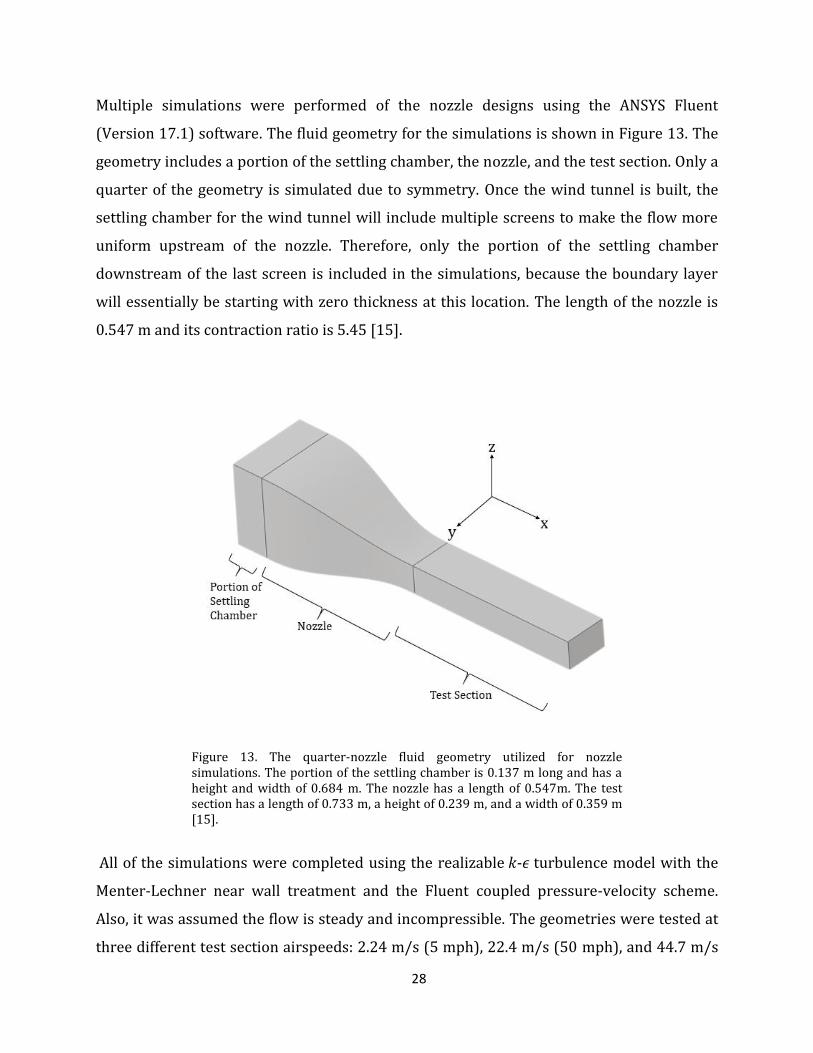
Multiple simulations were performed of the nozzle designs using the ANSYS Fluent

(Version 17.1) software. The fluid geometry for the simulations is shown in Figure 13. The

geometry includes a portion of the settling chamber, the nozzle, and the test section. Only a

quarter of the geometry is simulated due to symmetry. Once the wind tunnel is built, the

settling chamber for the wind tunnel will include multiple screens to make the flow more

uniform upstream of the nozzle. Therefore, only the portion of the settling chamber

downstream of the last screen is included in the simulations, because the boundary layer

will essentially be starting with zero thickness at this location. The length of the nozzle is

0.547 m and its contraction ratio is 5.45 [15].

Figure 13. The quarter-nozzle fluid geometry utilized for nozzle simulations. The portion of the settling chamber is 0.137 m long and has a height and width of 0.684 m. The nozzle has a length of 0.547m. The test section has a length of 0.733 m, a height of 0.239 m, and a width of 0.359 m [15].

All of the simulations were completed using the realizable 𝑘-𝜖 turbulence model with the

Menter-Lechner near wall treatment and the Fluent coupled pressure-velocity scheme.

Also, it was assumed the flow is steady and incompressible. The geometries were tested at

three different test section airspeeds: 2.24 m/s (5 mph), 22.4 m/s (50 mph), and 44.7 m/s

29

(100 mph). These speeds represent the range of airspeeds that will be produced in the test

section when the wind tunnel is in use. The quasi-one-dimensional continuity equation,

shown in Equation (22), was used to estimate the airspeed needed at the nozzle inlet to

achieve the specified airspeeds in the test section. These calculated airspeeds were set as the

inlet velocity boundary conditions for the inlet of the geometry. The outlet pressure boundary

condition is utilized to prescribe the flow to have a pressure equal to atmospheric pressure at

the outlet of the test section. Since the geometry used for the simulations is only a quarter of

the nozzle, the bottom and back walls of the geometry in Figure 13 were defined as symmetry

walls. It was specified that the fluid flowing through the nozzle was air that had a density of

1.225 kg/m3 and a viscosity of 1.79 × 10-5 kg/m∙s.

At first, simulations on the Bell and Mehta and Brassard nozzles were performed using a

coarse mesh (22,600 cells) and a fine mesh (181,000 cells). Thus, there were six

simulations completed for both nozzle geometries (three speeds and two meshes). For the

coarse mesh, the cells are approximately cubic with side lengths of 0.015 m except near the

walls where an inflation layer was used. There are five layers of cells in the inflation layer

and it has a total thickness of 0.015 m. The fine mesh, shown in Figure 14, has twice as

many cells in each direction than the coarse mesh does. The point of performing

simulations on the two meshes is to determine if the results vary depending on the chosen

mesh. Significant differences in the results would indicate that the simulations need to be

completed using a finer mesh in order to achieve accurate results. However, if the results

are approximately the same, then the specified meshes are fine enough. There were not

significant differences between the coarse and fine mesh simulation results, so only fine

mesh simulations were performed on the Morel nozzle.

After the simulations were finished, they were analyzed in ANSYS CFD-Post. For each case,

a plane was created at the start and end of the nozzle, as shown in Figure 15. The

stagnation pressure of the air at both planes was calculated using Equation (20). Then, the

difference in the area weighted average of the stagnation pressure between the two planes

was determined. This gave the loss of energy for the air as it moved through the nozzle.

Also, planes were created at various positions in the test section, as shown in Figure 15.

The equation

30

𝑢𝑥,𝑅𝑀𝑆 = √∫(𝑢𝑥 − 𝑢𝑥̅̅ ̅)2𝑑𝐴

𝐴

(35)

was used to determine the uniformity of the flow for each plane in the test section. In this

expression, 𝑢𝑥 is the streamwise component of the velocity, 𝑢𝑥̅̅ ̅ is the average streamwise

component of the velocity for the plane, and A is the area of the plane. The value for 𝑢𝑥,𝑅𝑀𝑆

for each plane was calculated in CFD-Post by creating a new expression. The expression

was defined as sqrt(areaInt((Velocity u – areaAve(Velocity u)@Plane)^2)@Plane /

area()@Plane), where Plane is the name of plane that the value of 𝑢𝑥,𝑅𝑀𝑆 is being calculated

for. Equation (35) gives the root-mean square of the difference between the streamwise

velocity and its mean over a given plane. Therefore, a lower 𝑢𝑥,𝑅𝑀𝑆 value corresponds to a

more uniform flow.

The planes at which the 𝑢𝑥,𝑅𝑀𝑆 values were calculated excluded the boundary layer region

near the nozzle and test section walls. This is because it is expected and acceptable for the

flow to be nonuniform in the boundary layer. It has been recommended that objects tested

in the wind tunnel should have a width less than 80% of the width of the test section [1].

Following this recommendation, the object will always be farther than 10% of the test

section width from any of the walls. For this reason, the planes created in the test section

excluded areas that are closer to the walls than 10% of the test section width.

31

Figure 14. Image of the fine mesh at the exit of the test section. This image is from the mesh that has 181,000 cells. The inflation layer, which contains 10 layers of cells, can be seen at the left edge and top of the image. The cells are smaller here to resolve the boundary layer that forms along the walls of the wind tunnel.

Figure 15. Image of planes created in the fluid geometry for simulation analysis.

32

Chapter 4

RESULTS AND ANALYSIS

In this chapter, results for the simulations using the fine grid detailed in the previous

chapter are shown and discussed. Three nozzles were tested based on the work of other

researchers: Bell and Mehta [13], Brassard [25], and Morel [12]. The data obtained from

the simulations were used to create Figure 16 through Figure 18. For the three nozzles,

these figures give information on the drop in stagnation pressure across them at different

air speeds and the flow uniformity in the test section.

Specifically, in Figure 16 the relationship between the stagnation pressure drop across the

nozzle and the average speed of the air in the test section is shown. It can be seen that at

low airspeeds the stagnation pressure loss across the nozzle is significantly smaller than at

higher airspeeds. This is expected based on dimensional analysis which shows that drag,

and therefore loss in stagnation pressure, should scale as the velocity squared. This trend

can be observed in Figure 16, but would be even more noticeable if more simulations,

especially ones at higher airspeeds, were performed. Although the trend is similar for each

nozzle, the Brassard nozzle performs the best followed by Bell and Mehta and finally Morel.

However, the differences between them are small, and any would be suitable based on this

measurement alone.

One final point to note about the data in Figure 16 is that the values for the loss in

stagnation pressure across the nozzles are about twice as large as the values estimated in

the preliminary phases of the design processes [15]. The reason for these discrepancies in

values most likely has to do with the fact that the previous estimates were obtained by

assuming each cross section of the nozzle behaves like a long cylindrical tube. This was

reasonable for the initial design of the wind tunnel but does not provide the most accurate

predictions. With that said, the under prediction of the stagnation pressure loss across the

nozzle is not expected to significantly affect the wind tunnel for a couple of reasons. First,

the preliminary estimates indicate that the stagnation pressure loss across the nozzle is

33

only about 3% of the total loss throughout the wind tunnel. Second, the estimations for

many of the other wind tunnel component losses were more conservative, which means

their actual stagnation pressure losses are likely to be lower than what was estimated.

Thus, since the under estimation calculated for the stagnation pressure loss across the

nozzle is a small percentage compared to the total losses, it will likely be covered by the

over estimations calculated for the other components.

Figure 16. Comparison of stagnation pressure loss for the three nozzles as a function of velocity. ūx,e is the area-weighted average streamwise velocity at the exit of the test section excluding the boundary layers.

Figure 17 shows a measure of the flow uniformity, calculated using Equation (35),

produced throughout the test section for each nozzle for the 2.24 m/s simulations.

Qualitatively similar results were obtained for the 22.4 m/s and 44.7 m/s simulations. In

fact, Figure 18 shows the results for all three speeds nearly overlap when they are

normalized relative to the area-averaged speed over each plane, �̅�𝑥. It can be seen from

these two graphs that the flow is less uniform at the start of the test section and becomes

more uniform as it travels downstream. At about x/L = 0.3 the flow uniformity levels out

and remains approximately constant throughout the rest of the test section. This is

acceptable because the test object will always be placed farther downstream than x/L = 0.3.

The flow uniformity asymptotes to about the same value for each of the nozzles. Figure 18

0

5

10

15

20

25

0 10 20 30 40 50

Stag

nat

ion

Pre

ssu

re D

rop

(P

a)

ūx,e (m/s)

Bell & Mehta

Brassard

Morel

34

shows that this value divided by the average air velocity is below 0.25%, which is the flow

uniformity criterion that is proposed by Mikhail [27]. Therefore, each of the nozzles

produce sufficient flow uniformity in the test section. When comparing the nozzles to each

other, the Brassard nozzle produces the lowest values and the Bell and Mehta nozzle the

highest. Also, at the start of the test section there is a noticeable difference in the flow

uniformity produced by each of the nozzles. The Morel nozzle produces the most uniform

flow at the start and the Brassard nozzle produces the least.

Based on the information obtained about the stagnation pressure loss and flow uniformity

of each nozzle, any of them would be acceptable. However, since the Brassard nozzle has

the lowest stagnation pressure drop and produces the most uniform flow after x/L =0.3, it

is the best nozzle design tested here.

Figure 17. Comparison of flow uniformity in the test section for different nozzles when 2.24 m/s (5 mph) flow was produced in the test section. This graph shows the RMS values of the variance in velocity of the flow at planes located at various positions in the test section. x is defined at the distance from the start of the test section and L is the length of the test section.

0

0.005

0.01

0.015

0.02

0.025

0.03

0.035

0.04

0.045

0 0.2 0.4 0.6 0.8 1

ux,

RM

S(m

/s)

x/L

Bell & Mehta

Brassard

Morel

35

Figure 18. Comparison of ux,RMS/ūx for the three simulations performed on each of the three nozzles. One simulation was conducted on each nozzle for the following airspeeds produced in the test section: 44.7 m/s, 22.4 m/s, and 2.24 m/s. The graph shows that for each nozzle the data from the three different simulations overlaps. L and x are defined in the caption of Figure 17.

0

0.2

0.4

0.6

0.8

1

1.2

1.4

1.6

1.8

2

0 0.2 0.4 0.6 0.8 1

ux,

RM

S/ū

x(%

)

x/L

Bell & Mehta

Brassard

Morel

36

Chapter 5

CONCLUSION

In this thesis, three nozzle designs were analyzed in order to determine which one is the

best for the wind tunnel being built at Houghton College. The three nozzle designs were

proposed in the papers by Bell and Mehta [13], Brassard [25], and Morel [12]. In order to

determine which nozzle is best, the stagnation pressure drop across the nozzle and the

flow uniformity produced in the test section was considered for each one. Based on these

criteria it was concluded that the Brassard nozzle is best. A possible reason for this is

because the Brassard nozzle has a larger inlet radius than outlet radius, while the other two

nozzles do not. This is the main characteristic unique to the Brassard nozzle that is

mentioned in Section 1.2 as being beneficial to the nozzle design. The Brassard nozzle

discussed here is only one out of a family of nozzles mentioned in Chapter 3 that have this

characteristic. Thus, additional tests could be completed to determine if a different type of

Brassard nozzle would perform better than the one discussed in this thesis. Other tests

could also be conducted to check for separation in the nozzles. In the research presented

here it was inferred that no separation occurred in the nozzle by studying the pressure and

velocity data produced from the simulations. However, no explicit tests were performed to

verify that separation did not occur. Thus, inviscid simulations could be conducted on each

nozzle and the Stratford Criterion (Section 2.3.3) could be used to explicitly check for

separation.

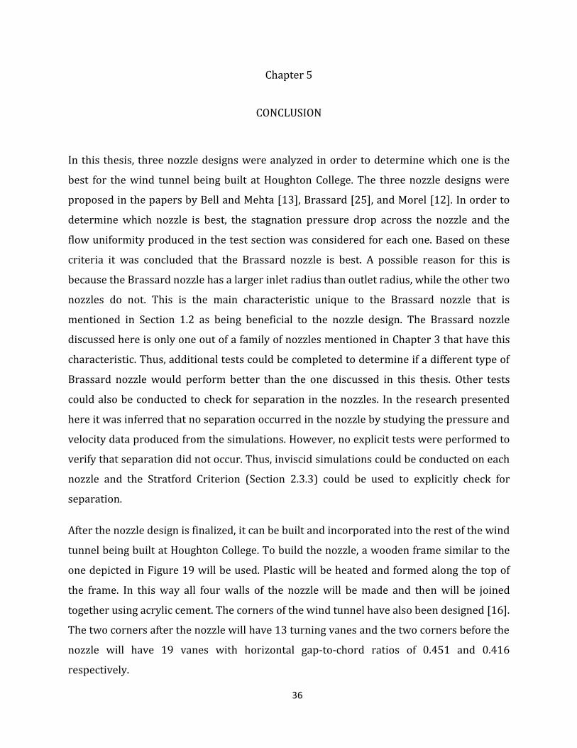
After the nozzle design is finalized, it can be built and incorporated into the rest of the wind

tunnel being built at Houghton College. To build the nozzle, a wooden frame similar to the

one depicted in Figure 19 will be used. Plastic will be heated and formed along the top of

the frame. In this way all four walls of the nozzle will be made and then will be joined

together using acrylic cement. The corners of the wind tunnel have also been designed [16].

The two corners after the nozzle will have 13 turning vanes and the two corners before the

nozzle will have 19 vanes with horizontal gap-to-chord ratios of 0.451 and 0.416

respectively.

37

A part of the wind tunnel that has yet to be designed is the balance system. This is what the

test object is affixed to and what allows researchers to measure forces and/or torques in

various directions. One possible approach is to construct a magnetic suspension balance

system [28]. This type of system uses electromagnets to suspend the test object in the air

without any physical supports (e.g., string or strut). By measuring the current supplied to

each of the electromagnets, the forces and torques acting on the test object can be

calculated. This type of balance system eliminates the issue of having physical supports in

the test section which affect the flowfield.

Figure 19. Picture of a wooden frame in the shape of the desired nozzle profile. The frame is made up of three profile forms (thick lines) connected by dowel rods (thin lines).

Once the wind tunnel is finished, it will be used to conduct research, primarily. There are

many different areas in which research could be performed using the wind tunnel as it is

designed for general purposes. One potential area of research that has been considered is

measuring how the aerodynamics of a wing are affected when ice forms on it. Specifically, it

would be interesting to study the wings of small unmanned aircraft because they are

gaining in popularity and the Houghton College wind tunnel will be ideally suited for

studying them. Also, at some point in the future, the wind tunnel can be used for

educational purposes including demonstrations and laboratory activities.

38

References

[1] J. Barlow, W. Rae, and A. Pope, Low-Speed Wind Tunnel Testing, 3rd ed. (Wiley-Interscience, New York, 1999). [2] Y. Li, Q. S. Li, and F. Chen, J. Wind Eng. & Industrial Aerodynamics, 167, 41-50 (2017). [3] A. Hedenstrom, and A. Lindstrom, J. Avian Biology, 48 (1), 37-48 (2017). [4] “Silhouette of an airplane” [Online]. Stock Pictures. http://www.stockpicturesforeveryone.com/2011/08/aircraft-sketches-and-silhouettes.html [5] J. Tannehill, D. Anderson, and R. Pletcher, Computational Fluid Mechanics and Heat Transfer, 2nd ed. (Taylor & Francis, Philadelphia, PA, 1997). [6] J. Slotnick, A. Khodadoust, J. Alonso, D. Darmofal, W. Gropp, E. Lurie, and D. Mavriplis, NASA CR 218178, 2014. [7] D. D. Baals and W. R. Corliss, Wind Tunnels of NASA, 1st ed. (Scientific and Technical Information Branch, National Aeronautics and Space Administration, Washington, D.C., 1981). [8] J. D. Anderson, Jr., A History of Aerodynamics, 1st ed. (Cambridge University Press, New York, 1999). [9] “Image of a whirling arm apparatus” [Online]. The Royal Society. http://prints.royalsociety.org/art/805939/whirling-arm [10] “An open return wind tunnel” [Online]. NASA. https://www.grc.nasa.gov/www/k-12/airplane/tunoret.html [11] “A closed return wind tunnel” [Online]. NASA. https://www.grc.nasa.gov/www/k-12/airplane/tuncret.html [12] T. Morel, J. Fluids Eng., 97 (2), 225-233 (1975). [13] J. H. Bell and R. D. Mehta, NASA CR 177488, 1988. [14] Y. Su, AIAA Journal, 29 (11), 1912-1920 (1991). [15] J. Jaramillo, Undergraduate Thesis, Houghton College, NY, 2017 (unpublished). [16] D. Eager, Undergraduate Thesis, Houghton College, NY, 2018 (unpublished). [17] I. G. Currie, Fundamental Mechanics of Fluids, 3rd ed. (CRC Press, Boca Raton, 2003). [18 ] J. D. Anderson, Jr., Fundamentals of Aerodynamics, 4th ed. (McGraw-Hill, New York, NY, 2007). [19] O. Zikanov, Essential Computational Fluid Dynamics, 1st ed. (John Wiley & Sons, Inc., Hoboken, NJ, 2010). [20] A. J. Smits and I. Marusic, Physics Today, 66 (9), 25-30 (2013). [21] M. Van Dyke, An Album of Fluid Motion, (The Parabolic Press, Stanford, CA, 1982). [22] B. S. Stratford, J. Fluid Mechanics, 5 (1), 1-16 (1959). [23] Wilcox, Turbulence Modeling for CFD, 3rd ed. (D C W Industries, La Cañada, CA 2006) [24] B. S. Stratford, Aero. Res. Council Reports & Memoranda No. 3002, 1957 (unpublished). [25] D. Brassard, J. Fluids Eng., 27, 183-185 (2005). [26] L. Leifsson and S. Koziel, J. Computational Science, 7, 1-12 (2015).

39

[27] M. N. Mikhail, AIAA Journal, 17 (5), 471-477 (1979). [28] H. Sawada, S. Suda, T. Kunimasu, presented at the 24th ICAS Congress, Yokohama, Japan, 2004 (unpublished).