NOVEL MACHINE LEARNING APPROACH FOR ANALYZING …

International Journal of Electronic Commerce Studies Vol.10, No.2, pp.175-202, 2019 doi: 10.7903/ijecs.1732

NOVEL MACHINE LEARNING APPROACH FOR ANALYZING ANONYMOUS CREDIT CARD FRAUD

PATTERNS

Sylvester Manlangit Charles Darwin University, NT, Australia

[email protected]

Sami Azam Charles Darwin University, NT, Australia

[email protected]

Bharanidharan Shanmugam Charles Darwin University, NT, Australia

[email protected]

Asif Karim Charles Darwin University, NT, Australia

[email protected]

ABSTRACT

Fraudulent credit card transactions are on the rise and have become a significantly problematic issue for financial intuitions and individuals. Various methods have already been implemented to handle the issue, but the embezzlers have always managed to employ innovative tactics to circumvent a number of security measures and execute the fraudulent transactions. Thus, instead of a rule-based system, an intelligent and adaptable machine learning based algorithm should be an answer to tackle such sophisticated digital theft. The presented framework uses k-NN for classification and utilises Principal Component Analysis (PCA) for raw data transformation. Neighbours (anomalies in data) were created using Synthetic Minority Oversampling Technique (SMOTE) and a distance-based feature selection method was employed. The proposed process performed well by having a precision and F-Score of 98.32% and 97.44% respectively for k-NN and 100% and 98.24% respectively for Time subset when using the misclassified instances. This work also demonstrates a larger and clearer classification breakdown, which aids in achieving higher precision rate and improved recall rate. In a view to accomplish such high accuracy, the original datum was transformed using Principal Component Analysis (PCA), neighbours (anomalies in data) were created using Synthetic Minority Oversampling Technique (SMOTE) and a distance based feature selection method was employed. The proposed process performed well when using the misclassified instances in the test dataset used in the previous work, while demonstrating a larger and clearer classification breakdown.

Keywords: Fraudulent Credit Card Transactions, k-NN, SMOTE, PCA, Machine Learning

mailto:[email protected]




176 International Journal of Electronic Commerce Studies

1. INTRODUCTION Credit card now days is responsible for transactions in the scale of billions of

dollars. 1 Global card business, in 2014 alone had a financial volume of around USD 28.84 trillion. 2 This meant that the importance of credit card has increased. These have become part of the financial systems. The convenience it has brought to consumers is one of the major factors. These can be used as substitute loan products. 3 In fact, credit cards are the key vehicle for the global e-commerce industry, which, as of 2017, was a USD 1.5 trillion industry in terms of turnover. 4

It is now a common process to pay with credit cards. 5 With the growth of credit card transactions, fraudulent transactions have also increased. It is not just a financial aspect, now a days Identity Fraud has also become a real concern. 6 Besides, with the ever-growing increase in online transaction, where the card actually remains unswept or absent physically, the rate of fraud is rocketing. For a note, online payment systems in 2015 have churned out more than $31 trillion worldwide, in the same line, credit card losses have accounted for $21 billion in the same year. 7 This rate is expected to grow by 51% by the year 2020. 8

Fraudulent transaction basically means, utilizing someone’s credit card without their knowledge or authorization. The perpetrator in most cases do not have any relation to the owner nor he\she ever intents to impart any knowledge about themselves or the process used in the embezzlement; the amount will never be returned as well. 9, 10 Merchants are more at risk than consumers. In the event of fraud, the merchant is one of the prime sufferers as his\her product is compromised. They often have to reimburse the chargeback fees and face the risk of closing their accounts. 10 These can lead to serious damage of reputation for the merchant and they can even face lawsuits of varying nature. 11

With the increase in the versatility of payment methods, new fraud patterns have emerged. This made the current fraud detection systems unsuccessful. 12 Another reason why fraud detection systems fail is that the persons committing fraud constantly change patterns when committing fraud, and this is the exact reason why the devised barrier against the fraudsters must employ machine learning concepts, not just to tackle, but also to address the phenomenon of “Concept Drift”. Stolen credit card information can often be used by the malicious agents to carry out transactions in the black market, where cryptocurrencies such as bitcoin, is already in heavy use. 13

As mentioned by Hand et al. 14, there are two levels of fraud protection. These are fraud prevention and fraud detection. Fraud preventions are things done to stop fraud from happening, while fraud detection pertains to detecting fraudulent transaction the moment they happen. 1 Innovation is needed for fraud detection because fraudsters are also evolving. 6

There are a number of critical factors in training the algorithm in fraud detection. 12 Further, public data is not always available due to the confidentiality issue. 15 The designed system also has to address factors such as non-stationary distribution of the data, decidedly imbalanced class distributions (skewed towards observations that are authentic) and unceasing streams of transactions. 15

From several studies, it is identified that the need for strictly accurate and high-performance fraud detection systems, based on automated machine learning principles, which can keep or even outpace the phenomena of “Concept Drift” in the problem

Sylvester Manlangit, Sami Azam, Bharanidharan Shanmugam and Asif, Karim 177

domain, is on the rise. Concept Drift refers to the change in behaviour of the fraudsters and methods applied over time. The existing rule-based static systems are all too behind the time to cope with the continuous cycle of innovative fraud methods of the crime gangs and thus leaves a lot to desire. To address this gap, this study proposes an advanced method based on feature selection of two of the most critical parameters and involves the usage of the k-NN algorithms for an effective classification to build the model. The appropriateness or fit of k-NN for the problem statement has been demonstrated in the previous studies and the model has been trained and tested in the present work.

2. RELATED WORKS 2.1 Fraud detection

Numerous researches have been carried out on fraud detection. One of these studies, compared the performance of each classification algorithm, such as Logistic Regression, Support Vector Machines and Random Forests, where Random Forest performed showed optimum performance. However, the selected attribute set that has been used for the experimentation, can actually be expanded even further to present a more accurate result. 6 Another study used feature engineering for detecting fraud, the researchers used the original features to create a pattern. An example was ‘Time’, a spending pattern was formed specifying the times a particular customer uses their credit card. But as the dataset used is proprietary, the discussion on specific features used, including the response and calculation time, is rather limited. 12 Other works range from the imbalanced dataset to creating new ways in improving fraud detection. 1, 15, 16 A study also showed data mining techniques used in fraud detection, some of the examples mentioned are clustering, classification and Neural Networks. Neural Networks have been found to be the most impactful, but the research also mentions the difficulty in developing systems based on Neural Network due to the lack of usable datasets. 17 One of the main issues with fraud detection is the involvement of growing large databases. 1 Another problem in fraud detection is the small number of fraudulent transactions compared to the normal transaction. The best algorithms resulted in many false positives (normal transactions classified as fraudulent transactions). 1 Lepoivre et al. demonstrated a system based on unsupervised methods such as PCA and SimpleKMeans (SKM) algorithm. 5 PCA has been used to represent transactions described by attributes such as amount, date etc. in a reduced subspace than the initial one, in a view to minimize information loss. Authors have clustered the data using SKM with impressive results. However, the test datasets were extremely limited and the system relies more on the execution time minimization rather than accuracy and precision. Therefore, it would be hard to deploy it in real situations as high accuracy as well as the precision in the final results are essential aspects of such sensitive automated processes. Table 1 provides a summary of the related works discussed for this study.


Table 1. A summary Overview of the Literature Review

Author Literature Research Focus

Outcome Identified Shortcoming

S. Bhattacharyya,

S. Jha, K. Tharakunnel

and C. Westland [6]

Data mining for credit card fraud: A

comparative study

The study compared the

performance of Logistic

Regression, Support Vector Machines and

Random Forests

Random Forest showed

better Performance

The selected attribute set could have been more

expanded

A. C. Bahnsen, D. Aouada, A.

Stojanovic and B. Ottersten

[12]

Feature engineering strategies for credit card

fraud detection

Feature

engineering for detecting fraud

Patterns for frauds have been created

using different features

Due to the proprietary nature of the dataset, the

discussion on specific features created has been

rather limited

K. Chaudhary and B. Mallick

[17]

Exploration of Data mining techniques in

Fraud. Detection:

Credit Card

Using clustering,

classification and Neural Networks in

fraud detection

Neural Networks performed optimally

The difficulty in developing

systems based on Neural Networks

M. R.

Lepoivre, C. O. Avanzini,

G. Bignon, L. Legendre, and A. K. Piwele

[5]

Credit card fraud detection

with unsupervised algorithms (Report)

Application of PCA and

SimpleKMeans (SKM)

algorithm

Better representation of features in

a reduced subspace

The test dataset was extremely

limited

Besides, Ref [1, 15 and 16] discusses issues such as handling imbalanced dataset and

creating new ways in improving fraud detection

Data mining is a widely used discipline in the fraud detection arena where analysis

of large datasets is accomplished to find unknown relationships between data and to present it in a way that it can be understood by the owner of the data, and this data must be useful. 14 This is also known as secondary data analysis. There are two types of methods in the analysis of the datasets, supervised and unsupervised. In supervised methods, it is assumed that past transactions are available and dependable, however, fraud patterns that have already taken place are often limited. 15 Unsupervised methods require slight or no prior classifications to anomalies. Hence, they are suitable for the transactions with no label. These methods mostly rely on Outliers- a basic but non-standard form of an observation. Stream Outlier Detection based on Reverse k-Nearest


Neighbours (SODRNN) 10, an unsupervised approach, uses the reverse K-Nearest Neighbours (k-NN) algorithm to detect the outliers and employs a datastream technique to carry out a single scan of the data instead of multiple times. However, the accuracy and precision of the model have not been measured and demonstrated clearly by the author, and the memory requirement needs to be managed with further efficacy to bring the model in a regular operable state. Prakash et al. presented a model based on semi-Hidden Markov Model (SHMM) that computes the distance between abnormal and normal processes, which is then taken into account to formulate the concept of Average Information Entropy (AIE) based on maximum entropy principle (MEP). 18 The model showed low data loss with improved precision and accuracy, but it works only on the user’s spending pattern, but fraud can take place from other aspects as well such as ‘geolocation’.

The prior work 2, which led to this study demonstrated that an amalgamation of undersampling techniques and Synthetic Minority Oversampling Technique (SMOTE) (discussed later) substantially increases the ‘Recall’ value of the classification algorithm used. k nearest neighbours (k-NN), has been found to be projecting the highest Recall compared to the other algorithms tested.

Now having taken the above knowledge into account, the work here introduces a framework based on k-NN, Principal Component Analysis (PCA) and SMOTE. Besides, a distance-based feature selection method has also been utilized for this novel machine learning based method to address the issue of fraud detection.

3. IMPLEMENTATION METHODS

3.1 Split test The dataset is divided into two parts, training set and test set. The size of the

training set can be defined by the user. Training set is the set of data used to train a model, specific features from this set is picked that is going to be put into the model. If done correctly, the model will be able to perform well when it is tested. 19 This acts as the raw material for the creation of the predicting model. All the details in the algorithm are based on the training set, this includes the model predictions.

‘Test’ set is the dataset that is going to be used to measure the performance of the prediction model. 19 The model is going to predict the classification of the test set based on what it has learned on the training set. Should the performance of the prediction model insufficient, it is suggested to adjust the model’s parameters. 19 Testing the model on the training set is not the right way, because the model knows the information. This creates misleading results. The model must be tested on data it has not seen. 19 3.2 Cross-Validation

Here the training and validation sets must cross-over in successive rounds for each data point is given a chance of being validated. The basic form of cross-validation is the k-fold cross-validation. In this cross-validation, the dataset is equally divided into k number of groups. The number of iterations is performed is same as k, where training and validation are performed. k -1 of the dataset are used for training and validation, while the rest of the dataset is used for testing the performance of the prediction model20.


3.3 Performance Measurement Below are some widely used principles for measuring the performance of a

prediction model: Confusion Matrix: Classification algorithms are usually assessed using the Confusion Matrix shown in Figure 1.

Predicted Negative

Predicted Positive

Actual Negative TN FPActual Positive FN TP

Figure 1. Confusion Matrix

In the above figure, the columns are the class predictor, while the rows are the actual class. TN (True Negative) stands for the number of correctly classified negative examples, FP (False Positive) denotes the number of misclassified positive samples. FN refers to the negative examples that are classified as positives, and TP is the samples of positives that are correctly classified. 21 In this research, fraudulent transactions have been marked as positive, while the non-fraudulent ones as Negative. Predictive accuracy may not be a good measure if the class imbalance is large. 21

Recall: The ratio of correctly classified positive instances to that of the total number of actual positive instances are termed as the Recall. Such measurement projects the capability of the classification algorithm in question to correctly classify the actual fraudulent instances. Equation 1 measures the percentage of fraud samples correctly classified as fraud. Recall = TP

TP FN+ (1)

Precision: Precision demonstrates the degree of true fraud instances out of the

predicted ones. Equation 2 measures the precision accuracy. Precision = TP

TP FP+ (2)

For performance analysis of the algorithm, both Recall and Precision will be

evaluated along with the F1 Score (using equation 3). F1 Score projects a better balance of the performance measure by taking both Precision and Recall into account. F1 Score = 2 x Precision*Recall

Precision Recall+ (3)


4. METHODOLOGY The first part of the study is to analyse the dataset. The aim is to understand what

anonymization process was used and how it transformed the data. After that original features ‘Time’ and ‘Amount’ will be broken down into separate groupings. This will give an insight into how many fraudulent transactions are present in each grouping, will be presented using a histogram. These groupings may be used in the training set size of the proposed process. A process for detecting fraud will be proposed. The proposed process will then be tested.

The first comparison will be between the dataset used in the initial analysis and the dataset size of the proposed fraud detection process. The next comparison will be using test data that has been misclassified in the initial analysis. A table will be shown for each comparison.

As suggested by Pozzolo et al. 15, a fraud detection system should have good ranking of transactions with their probability of being a fraud, rather than correctly classifying the transaction. The effectivity of the detection method will depend on how close it can predict the correct classification of the new data. The output of the suggested detection method should output the fraud probability of the new data, and it should also show how it reached the result.

The adopted methodology will include the PCA-transformation of the feature set to a sub-space with minimal information loss. The features “Time” and “Amount” will be left out of this process. Synthetic Minority Oversampling Technique (SMOTE) will then be applied to the selected training set. Grouping of features is the next step due to the reason as described in the beginning of this section. Once the grouping will be completed, k-NN will be applied for classification purposes, after which the results will be evaluated.

4.1 Anonymized credit card transaction dataset The dataset used in this research is from Kaggle.com. It is an anonymized credit

card data from European credit card users. It was anonymized to protect the privacy of the credit card users. The data has been distorted in a way that it will be impossible to identify any individual. Anonymization is the process of distorting data to preserve privacy. The dataset has numerical input variables that have been PCA transformed. 16 Principal Component Analysis (PCA) can be a basis for multivariate data analysis. One of the goals of PCA is finding a connection between each data. 22 PCA has transformed the original values into numbers, effectively hiding the privacy of the credit card users.

The concerned dataset has recorded a total of 284,807 transactions over a period of 2 days. Out of all the recorded transactions, 492 have been classified as fraud (0.172% of total transactions). The dataset is highly unbalanced. 16 According to Han et al. 23, two types of imbalances in a dataset are generally observed. The first one is between-class imbalance, this is an imbalance where one class have more samples than the other (as cited by Chawla), 21 and the other is within-class imbalance, where some subsets within the class have fewer samples than the others in the class. 24 The majority class is the class having lots of samples and the minority class is the one having fewer samples. 23 The dataset used in this research has an imbalance between classes. The fraudulent transactions, referred as the minority class, and the non-fraudulent transactions, which is the majority class. Sampling techniques have been suggested to address imbalanced datasets.


The dataset has 30 columns, features V1 to V28 are values that were PCA transformed to preserve confidentiality except for features such as “Time” and “Amount”. “Time” is the seconds elapsed from the first transaction in the dataset, and “Amount” is the transaction amount. The feature “Class” is the classification of the transaction, showing whether the transaction is a fraud. The research 16 pointed out that the “Amount” feature can be used for example-dependent cost-sensitive learning. This research may use “Time” and “Amount” features to find out any patterns that will lead to finding or detecting future fraudulent transactions. The features have been arranged from the highest to lowest, V1 having the highest variance, while V28 has the lowest variance as shown in Table 2. It is advised that, 16 measuring precision and recall accuracy by using the Area Under the Precision-Recall Curve (AUPRC). 4.2 Principal Component Analysis (PCA)

PCA allows a wide view of the relationship between credit card transactions, with calculations included. 5 This can be applied to very large datasets, in which this tool can handle regardless of the size and content. Another capability of the Principal Component Analysis (PCA) is transforming correlated variables into uncorrelated ones.

Table 2. Variance of each feature

Feature Variance Feature Variance Feature Variance v1 3.83649 v11 1.04186 v21 0.53953 v2 2.72682 v12 0.99840 v22 0.52664 v3 2.29903 v13 0.99057 v23 0.38995 v4 2.00468 v14 0.91891 v24 0.36681 v5 1.90508 v15 0.83780 v25 0.27173 v6 1.77495 v16 0.76782 v26 0.23254 v7 1.53040 v17 0.72137 v27 0.16292 v8 1.42648 v18 0.70254 v28 0.10896 v9 1.20699 v19 0.66266

v10 1.18559 v20 0.59433

In the case of credit card transactions, features of the original data are transformed into a smaller subspace without losing any information. 5 The transformation of the original data into a smaller subspace can also be described as the reduction of dimensions, which can easily be achieved using PCA. 25 If the original data is going to be reduced into one dimension, it has been suggested to create a principal component that has the most variation. 25 Another characteristic of PCA is that it expresses the data in a way that highlights its similarities and differences. Patterns in high-dimensional data are often hard to graphically represent, however, with the ability of PCA to reduce dimensions, analysis can be made much easier and intuitive. 26 4.3 Feature Selection

This is the process of analysing data and eliminate the attributes that do not


contribute to the result. There are two broad categories, these are the wrappers and filters. Wrappers evaluate features using algorithms and based on the resulting accuracy, the feature is eliminated or retained. Filters use a heuristic based evaluation of the features depending on the general characteristics of the data. 27 In the first part of the study, a feature will be used to build a classification model using the logistic regression algorithm. The results will be compared and check if there are features that can give higher fraud detection accuracy than the other features. 4.4 Checking the distribution of the fraudulent transactions

Time and Amount, two of the features that had not been transformed using PCA, will be used to divide the dataset into several classes and the distribution of the transactions will be noted. The breakdown will include the fraudulent transaction and the percentage of fraudulent transactions compared to the non-fraudulent transactions.

To determine the number of classes, Sturges’ rule will be employed. Sturges’ rule guides in the construction of a frequency curve or a histogram. 28 The goal of this section is to create a graph and see the distribution of the transactions, and determining the distribution of the transactions may provide additional information that would be useful in determining fraudulent transactions from non-fraudulent ones. 4.5 Using the ‘Time’ feature

The dataset contains credit card transactions in a span of two days. The unit of measure used in feature ‘time’ is in seconds. Pozzolo et al. 16 did not indicate the exact time of the day when the recording of the transactions started. The time in each transaction uses the first transaction as the reference point of the recording. Any transaction after 86,400 seconds will be referred as transactions that happened on the second day, and the last recorded transaction in the dataset has a time of 172,792 seconds. This fits within the total number of seconds in two days.

Table 3. Breakdown of the units of time

Count Units of Time 24 hours in a day 60 minutes in an hour 60 seconds in a minute

86400 seconds per day 172800 seconds in two days

Now using Sturges’ rule, the number of classes that are going to be used to

divide the transactions will be determined. Sturges’ rule is used to determine the number of class groupings when creating a histogram. The computation is given below:

Number of Classes = 1 + 3.3 log₁₀ n = 1 + 3.3 log₁₀ (86400) = 1 + 3.3(4.936514) Number of Classes = 17.29049535


The value of n is the total number of seconds in a day. The formula’s result is 17.29, rounding it off to 17. The histogram will have 17 groupings. These grouping may be used when proposing a new fraud detection process.

Next the class width has to be determined, this is to find out which transaction falls into what class. The smallest value refers to the starting second of the day, while largest value refers to the last second in a day (86400), these can be seen in Table 1. The formula used to determine the class width can be seen on the below calculation. The result gave us is 5082.35. This work will round-off the result to the nearest 100, making it 5100. The first class in Table 4 having 3 and 7 instances of fraud on the first two days respectively. These results will be used to divide the dataset.

Approximate Class Width = largest value - smallest value number of classes

=

86400 - 0 17

Approximate Class Width = 5082.352941

Table 4. Frequency distribution of the dataset using the feature 'time'

Class Limits Day 1 Day 2

Class MIN MAX Fraud Non-Fraud Fraud Non-Fraud 1 0 5100 3 5258 7 4783 2 5101 10200 22 2202 39 2356 3 10201 15300 13 2584 10 2497 4 15301 20400 13 1770 13 1428 5 20401 25500 10 2505 6 2950 6 25501 30600 24 5449 2 5922 7 30601 35700 9 10068 3 10057 8 35701 40800 14 11780 7 11791 9 40801 45900 45 11508 15 11377 10 45901 51000 13 10765 11 11013 11 51001 56100 18 11441 15 12174 12 56101 61200 21 10838 14 12257 13 61201 66300 17 11234 24 11768 14 66301 71400 17 11829 23 11314 15 71401 76500 10 12798 10 11053 16 76501 81600 14 13923 7 10295 17 81601 86400 18 8554 5 6774

Table 4 shows the lower limit and upper limit of each class, and the next column is the numbering of each class. Class 1 contains all the transactions that happened from 0 seconds to 5100 seconds on the first day and 86401 seconds to 91500 seconds. Each day has been divided into fraudulent and non-fraudulent transactions. According to Figure 2 class 2 to 5 have shown a higher percentage of fraudulent transactions compared to the other classes. The spike may have been affected by the


total number of non-fraudulent transactions. Compared to the other classes, class 2 to class 5, the total non-fraudulent transactions are between 3000 to 6000, while the other classes are around 20000 transactions.

Figure 2. Percentage of fraudulent transaction and total number of non-fraudulent transaction

This study tried to transform the unit of measure of seconds into hours in the day

assuming that the first recorded transaction happened on 12 midnight. Table 4 shows the converted values, and it provided additional insight as to why there were fewer transactions in the earlier classes because they happened on earlier parts of the day as this is mostly a non-working hour, thus not many people were active in carrying out the transactions. As demonstrated in Table 5, this timeframe has 17 classes.

Table 5. Converting seconds into hours in the day

MIN MAX Class MIN MAX Class 0:00 1:25 1 12:45 14:10 10 1:25 2:50 2 14:10 15:35 11 2:50 4:15 3 15:35 17:00 12 4:15 5:40 4 17:00 18:25 13 5:40 7:05 5 18:25 19:50 14 7:05 8:30 6 19:50 21:15 15 8:30 9:55 7 21:15 22:40 16 9:55 11:20 8 22:40 0:00 17 11:20 12:45 9

4.6 Using the ‘Amount’ feature

Now, the same process will be applied to the feature ‘Amount’. The information gained in this section might reveal characteristics of the fraudulent transactions. Using Sturges’ rule, this section will now determine the number of classes that are going to be used to divide the transactions. The computations are given below.


Number of Classes = 1 + 3.3 log₁₀ n = 1 + 3.3 log₁₀ (284807) = 1 + 3.3(5.454551) Number of Classes = 19.00001718

There will be 19 groupings in the feature “Amount”. n refers to the number of

transactions in the data set, which is 284, 807 transactions. In computing the class width, the result showed 1352.16. This will be rounded off to 1400. The largest value refers to the highest transaction value in the dataset, while the smallest value refers to the smallest valued transaction in the dataset.

Approximate Class Width = largest value - smallest value number of classes

= 25691.16 - 0 19

Approximate Class Width = 1352.166316

Table 6 shows there are four transactions not classified under class 1 of the feature ‘Amount’. Further breakdown is needed because 99.17% of the fraud transactions belong to Class 1 ($0 to $1400).

Table 6. Feature 'Amount' divided into 19 classes

Class limits Day 1 Day 2

Class MIN MAX Fraud Non-Fraud Fraud Non-Fraud 1 0 1400 279 143702 209 139076 2 1401 2800 2 632 2 574 3 2801 4200 0 124 0 105 4 4201 5600 0 30 0 29 5 5601 7000 0 10 0 12 6 7001 8400 0 4 0 7 7 8401 9800 0 1 0 1 8 9801 11200 0 0 0 2 9 11201 12600 0 1 0 1 10 12601 14000 0 1 0 0 11 14001 15400 0 0 0 0 12 15401 16800 0 0 0 0 13 16801 18200 0 0 0 0 14 18201 19600 0 0 0 1 15 19601 21000 0 1 0 0 16 21001 22400 0 0 0 0 17 22401 23800 0 0 0 0 18 23801 25200 0 0 0 0 19 25201 26600 0 0 0 1


Table 7 demonstrates the breakdown of transactions in 19 classes while the 20th

class contains the transactions in the range of $1426 to $26600, and it also showed that the first class of Table 6 contained 64.43% of the total fraudulent transactions in the dataset. A further breakdown is needed because more than 50% of the total fraudulent transactions are in a single class. The first class has been further broken in Table 8 with an interval of $4.

Table 7. Breakdown from $0 to $1425


Class MIN MAX Fraud Non-Fraud Fraud Non-Fraud 1 0 75 173 106698 144 105770 2 76 150 52 17308 24 15407 3 151 225 10 7206 8 6500 4 226 300 12 3890 6 3573 5 301 375 11 2220 9 2007 6 376 450 2 1555 1 1442 7 451 525 6 1152 2 1085 8 526 600 2 840 3 710 9 601 675 1 560 3 543 10 676 750 3 479 4 417 11 751 825 4 376 0 327 12 826 900 0 334 1 286 13 901 975 0 215 1 217 14 976 1050 0 258 1 243 15 1051 1125 0 153 1 138 16 1126 1200 0 167 0 147 17 1201 1275 1 123 0 109 18 1276 1350 0 89 1 100 19 1351 1425 3 109 0 82 20 1426 26600 1 774 2 706

Figure 3. Fraud Percentage of Each Amount Class Between $0 to $76


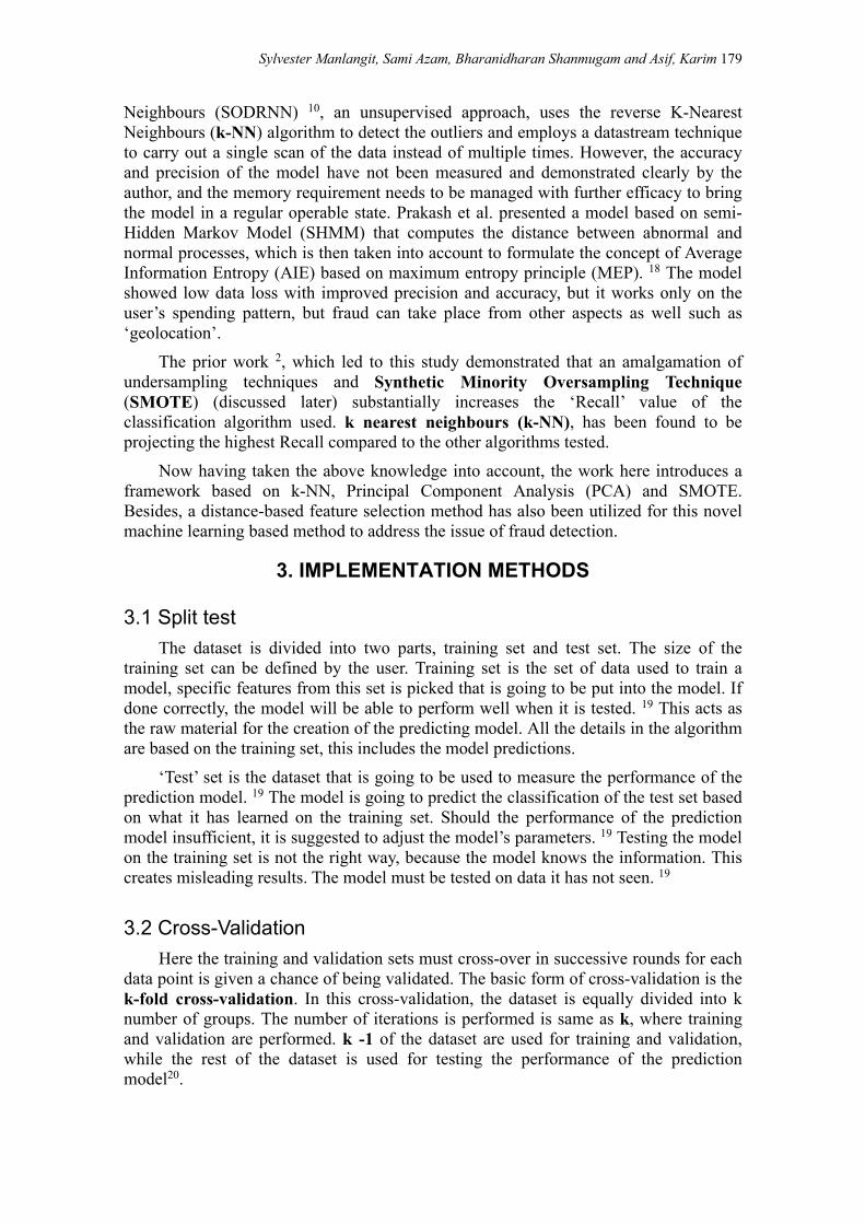
Table 8. Breakdown from $0 to $75


Class MIN MAX Fraud Non-Fraud Fraud Non-Fraud 1 0 4 127 33574 94 33668 2 5 8 12 10307 11 10534 3 9 12 6 12761 7 12689 4 13 16 2 7215 0 7342 5 17 20 7 6041 5 6192 6 21 24 2 4240 2 4128 7 25 28 0 3791 1 3701 8 29 32 6 4136 2 4162 9 33 36 1 3163 3 2881 10 37 40 2 3734 6 3590 11 41 44 0 2327 3 2152 12 45 48 3 2384 3 2446 13 49 52 0 2906 3 2882 14 53 56 1 1983 0 1823 15 57 60 4 2317 1 2228 16 61 64 0 1560 0 1390 17 65 68 0 1289 2 1116 18 69 72 0 1777 0 1629 19 73 76 1 1558 1 1505 20 77 26600 107 37443 67 33751

Table 8 shows most of the fraudulent transactions have the amount ranging from $0 to $4. This contained 44.92% of the total amount of fraudulent transactions. This small-valued transactions might be one of the causes for the loss of time and resources. Processing these small transactions causes the bank to allocate personnel to check the legitimacy of the transactions and merchant to pay fees for failed transactions or fraudulent transactions. The value of the transaction compared with the resources allocated is not balanced. As suggested by Pozzolo et al. 16 adding a cost-sensitive equation to the classification algorithm will enable it to increase the possibility of small-valued transaction with features that are similar to big-valued transactions. This will shorten the time of the investigation and it will allow the fraud analyst to focus on the bigger valued transactions or increased productivity when investigating small-value transactions.

5. PROPOSED NEW PROCESS

With the information gained in the earlier parts of the study, this section proposes a fraud detection method. Figure 4 sketches out the proposed framework.


Figure 4. Proposed process in detecting fraudulent transactions

The process starts when a new transaction comes in. This transaction will be PCA transformed in such a way that it follows the original dataset’s PCA transformation process, denoted as point 1 in Figure 4. A subset from the original dataset will be used as the training set of the classification of the new transaction. The subset will match with the class groupings using the feature ‘Time’ in Table 3, denoted as point 2 in Figure 4. The next process is to apply Synthetic Minority Oversampling Technique (SMOTE) to the fraud class of the selected subset, denoted as point 3 in Figure 4. SMOTE is an oversampling approach which, in place of carrying out oversampling with replacements, creates synthetic samples. These synthetic samples are presented along the line segments of the bona fide minority samples using the k minority class nearest


neighbours. Depending on the specified number of synthetic samples that need to be created, neighbours from the k nearest neighbours are randomly chosen. The purpose of SMOTE in this research work is to create neighbours for the fraudulent data. Next process is to create a grouping of features whose clustering distances are like each other, marked as point 4 in Figure 4. Classification will then be applied, using k-NN, with the value of k determined in the previous part of this research. 2 This is denoted as point 5 in Figure 4. Point 6 determines the classification decision of the classification algorithm. Each grouping will display the list of nearest neighbours based on k, with the distance and classification decision of each grouping, pointed out in Figure 4 as point 7.

5.1 Determining the training set for classification Grouping the dataset using the feature ‘Time’ and ‘Amount’ illustrated the

differences in the amount for transactions. The study on spending pattern by Jacobe and Jones 29 suggests that the spending pattern differs by age and gender. Dataset used in this study has been anonymized to keep the privacy of the details listed in the transaction. One of the challenges that this study has encountered is how to group the transactions with similar features. The only way to group the data is using the features, class, time and amount. It was shown in Table 3 and 8, that there were instances that fraudulent transaction increased at certain times and at different transaction amounts.

‘Time’ feature was used to determine the data that is going to be used as the training set. Based on the other researches on spending pattern, person creates a spending pattern based on certain times of the day. A working person who takes a break at 10 AM in the morning and uses a credit card to spend on a meal will have limited purchasing options and places they can spend or use the credit card. These transaction features, if transformed using PCA, will be plotted near to each other because these transactions have similar features, primarily because of this issue, the groupings done in Table 3 as the subset, will be used as the training set. 5.2 Application of SMOTE sampling technique The proposed fraud detection process will use SMOTE.

Figure 5. Fraud data is surrounded by non-fraud

Fraud data have been identified as an anomaly in the pattern, these are usually


alone, and these are surrounded by non-fraudulent data which can be seen in Figure 6. The fraudulent transactions are located inside the yellow circles as shown in Figure 5.

Since the process uses k-NN in classifying the test data, the nearest neighbours determine the classification of the test data. In Figure 5, it shows that three fraud data are surrounded by several non-fraud data. Although, k can have the value of 1, but is easily influenced by noise or unrelated data. Other sources suggest to use the formula, √n, where n is the number of fraud instances in the subset, when determining the value of k. 30

In Figure 6, there is an area between the fraud data and the surrounding non-fraudulent data. This is where the SMOTE samples will be placed, creating neighbours around the fraud data, and this creates a clustered area around it. If the test data fall within this area, then it can be interpreted as the test data having the same features as the fraudulent data.

Figure 6. Closer look at some fraud data surrounded by non-fraud data

5.3 Distance-based feature selection for grouping features In the proposed process, the creation of different grouping stemmed from

understanding how Random Forest algorithm worked and how it decides on classifying the test data. The different combination features give additional perspective while eliminate unrelated features and groups related features.

Using the tool ‘Orange’ 35, a linear projection of a subset in the dataset has been done and shown in Figure 7. It showed the fraudulent transactions in the subset are placed in a section of the linear projection. This indicated the idea of carrying out a feature selection that will enable each class to be clustered together, making it easier for the k-NN classification algorithm to perform better. In Figure 5, some of the fraudulent data are within the non-fraudulent data. When comparing the structure of the linear projections between Figure 7 and Figure 8, it demonstrates that feature selection will improve the accuracy or performance of the fraud detection process.


Several studies have explained and used several feature selection methods. Examples of these methods are Information Gain, Gain Ratio and Correlation based Feature Selection (CFS). 31 These methods are used in other classification algorithms, Information Gain and Gain Ratio have been used mostly in Decision Trees. This type of selection selects the best feature in splitting the decision tree.

The proposed process uses the k-NN algorithm to classify a test data or a new transaction. This study will follow the distance-based feature selection method proposed by Kim et al. 32 for feature selection in fault detection prediction model. The model has two outcomes, which is similar to fraud detection. The method uses the Euclidean distance formula, the mean absolute value and standard deviation of each feature. Mean absolute value (MAV) refers to average distance of the values from the mean. 33 and standard deviation (SD) refers to how far are the values to the mean. 34 These statistical measures group feature based on how clustered they are; this would separate features whose data are clustered and data that are spread out. Equation 4 is used for calculating the distance between features.

Figure 7. Class 1 in time group, using features V14, V12, V11 and V4

.

𝒹𝒹 = ( ) ( )2 2

? ? ? ?feature feature feature featureMAV MAV SD SD− + − (4)


Figure 8. Linear projection of class 1 in time group using all the features

Upon using the proposed feature selection method, using the class 1 grouping in the feature ‘Time’, Table 9 showed the top 10 features that have the shortest distance in relation to the other features. In columns labelled 2 to 10, these are the features whose distance is close to the primary feature in column labelled ‘feature’. These groupings will be used in the classification process when applying the k-NN algorithm.

Table 9. Top 10 features with shortest total distance regarding the other features

Ranking Primary

Distance Nearest Neighbouring Features

Feature 1 2 3 4 5 6 7 8 9 10 1 v15 8.31885 15 14 16 7 19 21 17 11 18 9 2 v14 8.31885 14 7 11 9 15 10 8 13 16 19 3 v7 8.36454 7 11 14 9 10 15 8 13 5 16 4 v11 8.42525 11 7 9 14 10 8 13 15 5 16 5 v16 8.53435 16 19 21 17 18 22 15 20 14 24 6 v19 8.56594 19 21 17 16 18 22 15 20 24 14 7 v21 8.59045 21 17 19 16 18 22 15 20 24 14 8 v17 8.59751 17 21 19 16 18 22 15 20 24 14 9 v9 8.61544 9 10 11 7 8 14 13 5 15 12 10 v10 8.81429 10 9 8 13 11 7 14 5 15 12

Upon checking the groupings, there are features that were repeatedly used, shown

in Table 10 However, there were features that were missed and not included in the groupings. When Random Forest performed feature groupings, it used all the features when classifying the test data. This study wants to make sure that when detecting fraud, the process should use all features, but place these into different groupings. The other features are ranked in the lower parts of the table.


Table 10. Features repeatedly used, while some features were not used

Primary feature Features selected for each grouping v15 7 8 9 10 11 13 14 15 16 17 18 19 20 21 22 v14 5 7 8 9 10 11 13 14 15 16 17 18 19 21 22 v7 5 7 8 9 10 11 12 13 14 15 16 17 18 19 21 v11 5 7 8 9 10 11 12 13 14 15 16 17 18 19 21 v16 7 8 9 10 11 14 15 16 17 18 19 20 21 22 24

5.4 Presenting the classification result The result of the fraud detection process is the list of nearest neighbours for each

grouping. The number of neighbours will be defined by k, when the classification algorithm was performed, the summary for each group will have the count of neighbours for each class, total distance and average distance. The result will give the fraud analyst additional insight. This study will hold onto some of the suggestions suggested in one the studies 15 that a sound fraud detection system should rank the transaction with its possibility as a fraudulent transaction, instead of classifying a transaction correctly. The breakdown of the classification decision enables the fraud analyst to see the related training data to the test data.

The proposed fraud detection process should be able to classify better than the classification algorithms presented in the initial analysis. 2 It will be tested using the dataset used by different classification algorithms for comparison, and the second part of the testing is to get a misclassified instance in the initial analysis 2 and test it on the proposed fraud detection process. If the proposed process can show a breakdown of the classification decision that can classify the selected instance correctly, then this research would assume that the proposed fraud detection process works as expected.

6. RESULTS In this section, the proposed process will be compared with the results obtained

from the usage of a classification algorithm with a tool. Following are the sampling techniques used on the dataset (Table 11).

Table 12 shows a comparison between the performance of the k-NN classification algorithm and performance achieved using the time groupings of the dataset with the same applied settings. The precision has increased when using the time grouping, example used was the class 1 grouping. Although there was a decrease in recall accuracy, but comparing the size of the misclassified data, it is found to be lower because the original subset contains fewer fraud data compared to the whole dataset. The proposed grouping also prevents characteristics of unrelated data from getting mixed in with the test data. This section interprets the finding as preventing the regular spending pattern at certain times from other time-groupings from admixing with fraud pattern present in the selected time-grouping.


Table 11. Settings used in k-NN classification algorithm

Applied Sampling Techniques SMOTE k-NN 6 Samples Added 1000% Undersampling Ratio 1:1

Classification Algorithm k-NN Nearest neighbours 7 Distance Formula Euclidean Weight Uniform Implementation Split Test Training Set 70% Test Set 30%

Table 12. Comparison between k-NN classification algorithm and a time subset grouping

Comparison TP FN TN FP Precision Recall F-Score k-NN 1583 27 1581 56 98.32% 96.58% 97.44%

Time sub-set Class 1 28 0 37 1 100.00% 96.55% 98.24%

This choice of grouping has resulted in the enhancement of the performance in using the k-NN algorithm in general. Furthermore, there are studies that declared the importance of grouping data that have similar features. 1, 6. 12, 15, 17

The next stage of comparison will evaluate if the proposed process produces a different classification or decision using a misclassified instance in the same dataset. The initial test has a 70/30 split test, using 30% of the data as the test data in checking the accuracy of the model. A misclassified instance in the test set will be used to check if there are changes in the classification decision or will it still misclassify the selected instance. Table 13 shows the details of the misclassified instance in the initial analysis. 2 Tools such as ‘Orange’ and ‘Weka’ can display the instances in the test set, the original classification and the classification algorithm’s class prediction.


Table 13. A misclassified instance in the test set

Data Count UniqueID Time Actual

Class Predicted Classification

kNN Random Logistic 2863 57320.5 48313.7 Fraud Non-Fraud Non-Fraud Non-Fraud

Following the proposed process, a subset of the dataset used to classify the selected instance will be used to identify the nearest neighbours. The time of the selected instance is 48313.69189, this falls in the 9th class or grouping in the ‘Time’ feature. The range of the grouping is from 40801 seconds to 45900 seconds. The next process is to determine the groupings, five of these. Table 14 shows the groupings of feature when the classification process is implemented. All the features were present in one of the groupings.

Table 15 shows the summary of each grouping compared to the whole dataset. Using the dataset used in the initial analysis, the nearest neighbours of the selected instance were divided into 3 Frauds and 4 Non-Frauds.

Table 14. Groupings that is going to be used for the classification process

Primary Feature Features selected for each grouping

v16 8 9 10 11 13 14 15 16 17 18 19 20 v11 7 8 9 10 11 13 14 15 16 17 18 19 v2 1 2 3 4 5 6 7 8 9 10 11 13 v27 12 14 16 17 18 19 20 21 22 23 24 25

Therefore, the algorithm has classified it as a non-fraud because there are more non-fraud neighbours compared to the fraud neighbours. In the case of the proposed process, all the groupings have shown that it leans to the fraud class. It also meant that the proposed process does work while correctly classifying a data.

Table 14 also indicates that the fraud neighbours are closer to the tested instance. Group 4 showed the nearest distance, which is 0.98. The non-fraud neighbours in the proposed process displayed a shorter distance compared to the non-fraud neighbours in the initial analysis.

The initial analysis showed greater number of non-fraud neighbours compared to the fraud neighbours. In the feature groupings, groups 1, 3 and 4 showed the nearest neighbours of the tested instance belong to the fraud class. Group 2 is the only feature grouping that showed non-fraud neighbours, and the grouping showed that there are more fraud neighbours compared to the non-fraud.


Table 15. Classification summaries for each grouping and the whole dataset

Attribute

k-NN Group 1 Group 2 Group 3 Group 4

Fraud

Non-

Fraud

Fraud

Non-

Fraud

Fraud

Non-

Fraud

Fraud

Non-

Fraud

Fraud

Non-

Fraud

Count 3 4 7 0 4 3 7 0 7 0 Total Distance 4.76 9.15 9.82 0.00 6.26 5.98 10.10 0.00 6.85 0.00

Average Distance 1.59 2.29 1.40 0.00 1.57 1.99 1.44 0.00 0.98 0.00

7. CONCLUSION

Based on the finding in the prior research work, an intelligent machine learning based framework has been developed in this current study to effectively combat the issue of credit card fraud detection. It achieved an F-Score of 97.44% with precision and recall of 98.32% and 96.58% respectively. The model employs k-NN, Principal Component Analysis (PCA) and SMOTE along with a distance-based feature selection method has also been introduced. The proposed process used smaller training set. This reduced the training and testing time of the classification algorithm, as well as the resources needed to perform the algorithm. Application of smaller subset cut down the number of misclassified instances, because the instances are grouped in such a way where spending characteristics are time specific. The proposed process performed commendably when using the misclassified instances in the test dataset used in the initial analysis. 2 The process demonstrated a larger and clearer classification breakdown. However, there were misclassified instances that portrayed the same results. This study identified one possible reason for the misclassification, which is the SMOTE instances were too many. This resulted in allowing the fraudulent data to get mixed with the non-fraudulent ones.

The dataset used in this study showed features that separated the fraudulent and non-fraudulent data. This helped the classification algorithms in creating models with high fraud detection accuracy. On the other hand, there were features that clearly mixed both classes. The reason Random Forest and Logistic Regression could produce good results was the combination of all features. It used the features that clearly separated the classes as the main identifier of the fraudulent class while using the other features as the gradient separator. The structure of the features helped in the creation of the fraud detection method. This study concludes that the interpretation of the dataset directly affects the fraud detection process. Without factors or features that help separate a fraud from a non-fraud transaction, the difficulty in detecting fraud becomes a difficult task.

8. FUTURE WORK The success in classifying the misclassified instances of k-NN classification

algorithm by the proposed fraud detection process presented in this study showed promise. However, there are rooms for improvements such as having a different number of fraudulent transactions each time grouping is done. Further, the percentage value of


SMOTE needs to be identified correctly. The comparison of results only tested the misclassified instances in the test data. This study did not cover the effects of the quantity of the SMOTE instances. The main reason for using SMOTE is to create an area for the single fraud instances. This is one of the future works of this study.

Transforming the new data into PCA format is part of the proposed process. The process of using PCA on to the new data needs to be studied, as the original data has been concealed, there is a need to know how PCA can affect the performance of a dataset and the possibility of information gain or loss when transforming a dataset.

The transformation of the dataset into numerical form added to the effectivity of the k-NN algorithm. This study has defined fraud as anomaly in the spending pattern of a person. The possibility of this happening regularly is under 1% in a group of 280,000 transactions. Using this definition, new data that has the same features or numerical value as the recorded fraudulent transaction in the same time grouping will classify the new data as a fraudulent transaction.

To check the proposed process on to other binary result dataset is another objective for the future. This is to see if it will perform in detecting the positive class of the dataset. If the performance of the proposed process is high, this could be interpreted that the proposed process is applicable to binary result dataset using time series groupings.


9. REFERENCES

[1] S. Jha and C. Westland, A Descriptive Study of Credit Card Fraud Pattern. Global Business Review, 14(3), p373-84, 2013. https://doi.org/10.1177/0972150913494713

[2] S. Manlangit, S. Azam, B. Shanmugam, K. Kannoorpatti, M. Jonkman and A. Balasubramaniam, An efficient method for detecting fraudulent transactions using classification algorithms on an anonymized credit card dataset. Intelligent Systems Design and Applications, Springer, 736, p418-429, 2018. https://doi.org/10.1007/978-3-319-76348-4_41

[3] J. M. Liñares-Zegarra and J. O. S. Wilson, Credit card interest rates and risk: new evidence from US survey data. The European Journal of Finance, 20(10), p892-914, 2014. https://doi.org/10.1080/1351847X.2013.839461

[4] Statistica. e-Commerece. Retrieved from: https://www.statista.com/outlook/243/100/ecommerce/worldwide#, 2018.

[5] M. R. Lepoivre, C. O. Avanzini, G. Bignon, L. Legendre, and A. K. Piwele, Credit card fraud detection with unsupervised algorithms (Report). Journal of Advances in Information Technology, 7(1), 34, 2016. https://doi.org/10.12720/jait.7.1.34-38

[6] S. Bhattacharyya, S. Jha, K. Tharakunnel and C. Westland, Data mining for credit card fraud: A comparative study. Decision Support Systems, 50(3), p602-613, 2011. https://doi.org/10.1016/j.dss.2010.08.008

[7] C. Jiang, J. Song, G. Liu, L. Zheng and W. Luan, Credit Card Fraud Detection: A Novel Approach Using Aggregation Strategy and Feedback Mechanism. IEEE Internet of Things Journal, March, 2018. https://doi.org/10.1109/JIOT.2018.2816007

[8] NilsonReport. retrieved from: The Nilson Report: https://www.nilsonreport.com/upload/content promo/The Nilson Report 10-17-2016.pdf, October, 2016.

[9] A. Prakash and C. Chandrasekar, A parameter optimized approach for improving credit card fraud detection. International Journal of Computer Science Issues, 10(1), p360-366, 2013.

[10] V. R. Ganji and S. N. P. Mannem, Credit card fraud detection using anti-k nearest neighbor algorithm. International Journal on Computer Science and Engineering, 4(6), p1035-1039, 2012.

[11] R. Elitzur, Y. Sai, A Laboratory Study Designed for Reducing the Gap between Information Security Knowledge and Implementation. International Journal of Electronic Commerce Studies, 1(1), p37-50, 2010.

[12] A. C. Bahnsen, D. Aouada, A. Stojanovic and B. Ottersten, Feature engineering strategies for credit card fraud detection. Expert Systems with Applications, 51, p134-142, 2016. https://doi.org/10.1016/j.eswa.2015.12.030

[13] J. Jose, K. Kannoorpatti, B. Shanmugam, S. Azam, K. Yeo, A Critical Review of Bitcoins Usage by Cybercriminals. International Conference on Computer Communication and Informatics (ICCCI), India, 2017.

[14] D. J. Hand, H. Mannila and P. Smyth, Principles of data mining, MIT Press, 2001. [15] A. D. Pozzolo, O. Caelen, Y. L. Borgne, S. Waterschoot and G. Bontempi, Learned

lessons in credit card fraud detection from a practitioner perspective. Expert Systems with Applications, 41(10), p4915-4928, 2014. https://doi.org/10.1016/j.eswa.2014.02.026

[16] A. D. Pozzolo, O. Caelen, R. A. Johnson and G. Bontempi, Calibrating Probability with Undersampling for Unbalanced Classification. In IEEE Symposium Series on


Computational Intelligence, pp: 159-166, 2015. https://doi.org/10.1109/SSCI.2015.33

[17] K. Chaudhary and B. Mallick, Exploration of Data mining techniques in Fraud. Detection: Credit Card. International Journal of Electronics and Computer Science Engineering, 1(3), p1765-1771, 2012.

[18] A. Prakash, and C. Chandrasekar, A Novel Hidden Markov Model for Credit Card Fraud Detection. International Journal of Computer Applications, 59(3), p35-41, 2012.

[19] R. West. Training Set vs. Test Set. Retrieved from: http://content.nexosis.com/blog/training-set-vs.-test-set, 2016.

[20] P. Refaeilzadeh, L. Tang and H. Liu, Cross-validation. Encyclopedia of database systems, Springer, p532-538, 2009.

[21] N. V. Chawla, Data mining for imbalanced datasets: An overview. Data mining and knowledge discovery handbook, Springer, Chap:40, 2015. https://doi.org/10.1007/978-0-387-09823-4_45

[22] S. Wold, K. Esbensen and P. Geladi, Principal component analysis. Chemometrics and intelligent laboratory systems, 2(1-3), p37-52, 1987. https://doi.org/10.1016/0169-7439(87)80084-9

[23] H. Han, W. Wang and B. Mao, Borderline-SMOTE: a new over-sampling method in imbalanced datasets learning. Advances in intelligent computing, p878-887, 2005. https://doi.org/10.1007/11538059_91

[24] G. Weiss, Mining with rarity: A unifying framework. SIGKDD Explorations, 6(1), p7-19, 2004. https://doi.org/10.1145/1007730.1007734

[25] V. Powell, Principal Component Analysis. Retrieved from: http://setosa.io/ev/principal-component-analysis/, 2015.

[26] L. I. Smith, A tutorial on Principal Components Analysis. Information Fusion, 51, 52, 2002.

[27] S. Nadarajan and B. Ramanujam, Encountering imbalance in credit card fraud detection with metaheuristics. Advances in Natural and Applied Sciences, 10(8), p33-42, 2016.

[28] D. W. Scott, Sturges' rule. Wiley Interdisciplinary Reviews: Computational Statistics, 1(3), p303-306, 2009. https://doi.org/10.1002/wics.35

[29] D. Jacobe and M. Jones, Consumers Spend More on Weekends, Payday Weeks; Average daily spending is lowest at beginning of work week, (Survey). Gallup Poll News Service, 2009.

[30] T. Srivastava, Introduction to k-nearest neighbours : Simplified. Retrieved from: https://www.analyticsvidhya.com/blog/2014/10/introduction-k neighbours-algorithm-clustering/, 2014.

[31] J. Novaković, Toward optimal feature selection using ranking methods and classification algorithms. Yugoslav Journal of Operations Research, 21(1), p119-135, 2016. https://doi.org/10.2298/YJOR1101119N

[32] J. Kim, Y. Han and J. Lee, Data Imbalance Problem solving for SMOTE Based Oversampling: Study on Fault Detection Prediction Model in Semiconductor Manufacturing Process. Advanced Science and Technology Letters (Information Technology and Computer Science), 133, p79-84, 2016. http://dx.doi.org/10.14257/astl.2016.133.15

[33] D. Roberts, Mean Absolute Deviation. Retrieved from: https://mathbitsnotebook.com/Algebra1/StatisticsData/STMAD.html.

[34] D. Roberts, Variance and Standard Deviation. Retrieved from: https://mathbitsnotebook.com/Algebra1/StatisticsData/STSD.html.


[35] Orange Data Mining. Linear Projection. Retrieved from: https://docs.orange.biolab.si/3/visual- programming/widgets/visualize/linearprojection.html

https://docs.orange.biolab.si/3/visual-%20programming/widgets/visualize/linearprojection.html

https://docs.orange.biolab.si/3/visual-%20programming/widgets/visualize/linearprojection.html

NOVEL MACHINE LEARNING APPROACH FOR ANALYZING …

Documents

Transcript of NOVEL MACHINE LEARNING APPROACH FOR ANALYZING …