notes part 3 - UBCcourses.ece.ubc.ca/359/notes/notes_part3.pdfEECE 359 - Signals and Communications:...

EECE 359 - Signals and Communications: Part 3 Spring 2014

Introduction to probability with applications

in communications1

Probability theory is useful in many areas

of engineering in which uncertainty plays

an important role, e.g. noisy signals in a

communication system.

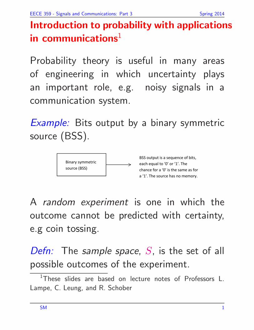
Example: Bits output by a binary symmetric

source (BSS).

Binary symmetric

source (BSS)

BSS output is a sequence of bits,

each equal to ‘0’ or ‘1’. The

chance for a ‘0’ is the same as for

a ‘1’. The source has no memory.

A random experiment is one in which the

outcome cannot be predicted with certainty,

e.g coin tossing.

Defn: The sample space, S, is the set of all

possible outcomes of the experiment.1These slides are based on lecture notes of Professors L.

Lampe, C. Leung, and R. Schober

SM 1


Example: For an experiment in which two

coins are tossed,

S = {(H,H), (H,T ), (T,H), (T, T )}.

Example: For an experiment in which two

dice are tossed,

S = {(i, j) : i, j = 1, 2, 3, 4, 5, 6}

where i (j) appears on the first (second) die.

Defn: An event, A, is some subset of S.

Event A is said to have occurred if the

outcome of the experiment is contained in

A.

An axiomatic approach to probability theory

is possible. Here, we adopt a commonly used

engineering approach.

SM 2


Defn: The probability of an event A is

P (A) = limn→∞

(nA

n

)

(1)

where nA is the number of occurrences of A

in n trials.

Example: Suppose that we toss a coin 100

times and a head (H) comes up 51 times.

Then, P (H) ≈ 0.51.

Example: Consider a sequence of three bits

output by a BSS. What is the probability that

the sequence contains two consecutive 0’s?

Example: Lotto 6/49. What is the probability

of a given ticket winning the jackpot?

From (1), we conclude that

0 ≤ P (A) ≤ 1 (2)

for any event A. If A = ∅, i.e. a null

SM 3


event, P (A) = 0; if A = S, i.e. a sure event,

P (A) = 1.

Defn: The union of two events A and B,

denoted by A ∪B, is the event consisting of

all outcomes that are either in A or in B or

in both A and B.

Example: In the two coin tossing experiment,

let A be the event that the first coin shows

a head, i.e. A = {(H,H), (H,T )} and let

B = {(T,H)}. Then,

A ∪B = {(H,H), (H,T ), (T,H)}

i.e. the event that we have one head on

either coin.

Defn: The intersection of two events A and

B, denoted by AB or A ∩B, is the event

consisting of all outcomes that are in both A

and B.

SM 4



let A be the event that at least one head

occurs, i.e. A = {(H,H), (H,T ), (T,H)}and let B be the event that at least one tail

occurs, i.e. B = {(H,T ), (T,H), (T, T )}.Then,

AB = {(H,T ), (T,H)}i.e. the event that we have exactly one head

and one tail.

Defn: Two events, A and B, are said to be

mutually exclusive or disjoint if AB is a null

event, i.e. AB = ∅.


let A be the event that the first coin shows

a head, i.e. A = {(H,H), (H,T )} and let B

be the event that the first coin shows a tail,

i.e. B = {(T,H), (T, T )}. Then,

AB = ∅.SM 5


Fact: If two events, A and B, are mutually

exclusive, then

P (A ∪B) = P (A) + P (B) (3)

Proof:

Defn: The complement of an event A,

denoted by Ac, is the event consisting of

all outcomes in S that not in A. Thus, Ac

occurs if and only if A does not occur.

Example: In the one coin tossing experiment,

let A be the event that the coin shows a head.

Then, Ac is the event that the coin shows a

tail.

Note that Sc = ∅ since the experiment always

results in some outcome.

Fact: If B ⊂ A, then P (B) ≤ P (A).

SM 6


Defn: The probability of a joint event, AB,

is

P (AB) = limn→∞

(nAB

n

)

(4)

where nAB is the number of occurrences of

the event AB in n trials.

Theorem:

P (A ∪B) = P (A) + P (B)− P (AB) (5)

Proof:

Defn: The conditional probability that an

event A occurs given that an event B has

occurred is

P (A|B) =P (AB)

P (B)(6)

SM 7


provided P (B) > 0.

From (6), we have

P (AB) = P (A)P (B|A)

= P (B)P (A|B) (7)

Defn: Events A1, A2, . . . , An are said to

form a partition of the sample space S if

1. A1, A2, . . . , An are mutually exclusive, i.e.

Ai

⋂

Aj = ∅ for i 6= j.

2. A1 ∪A2 ∪ . . . ∪An = S.

Total Probability Theorem: LetA1, A2, . . . , An

form a partition of S. Then, for any event B,

P (B) =n∑

i=1

P (B|Ai)P (Ai) (8)

SM 8


Using (7) and (8), we can write

Theorem (Bayes):

P (A|B) =P (B|A)P (A)

P (B)

=P (B|A)P (A)

∑ni=1P (B|Ai)P (Ai)

(9)

Example: Binary asymmetric channel

The input bit, X, is equally likely to be 0 or

1, i.e. P (X = 0) = P (X = 1) = 12.

Determine(a) P (X = 0|Y = 0).(b) P (X = 1|Y = 1).

SM 9


Example: Breathalyzer

Suppose that 10% of the drivers on the

road after midnight are legally drunk. A

police officer stops a driver at random and

administers the breathalyzer test.

SM 10


Suppose that

Pr{test indicates driver is drunk | driver is drunk}=0.95 and

Pr{test indicates driver is drunk | driver is not drunk}=0.01

What is the probability that the driver is drunk

given that the test is positive, i.e. indicates

the driver is drunk?

Solution:

Let A1 be the event that the driver is drunk,

A2 be the event that the driver is not drunk

and B be the event that the test is positive.

Then, from Bayes’ Theorem (9),

P (A1|B) =P (B|A1)P (A1)

P (B|A1)P (A1) + P (B|A2)P (A2)

=0.95× 0.1

0.95× 0.1 + 0.01× 0.9≈ 0.91

Defn: Two events A and B are said to be

SM 11


independent if

P (AB) = P (A)P (B) (10)


let A be the event that the first coin shows a

head and let B be the event that the second

coin shows a tail. Then,

P (A) =1

2

P (B) =1

2

P (AB) =1

4

Thus, the event that the first coin shows

a head is independent of the event that the

second coin shows a tail.

SM 12


Random variables

Defn: A real-valued random variable (rv) is a

function which associates a real number X(s)

with each possible outcome s in the sample

space S.

Example: In the coin tossing experiment,

X(H) = +1

X(T ) = −1

Cumulative distribution and probability

density functions

Defn: The cumulative distribution function

(CDF) of the rv X is

FX(x) = P (X ≤ x) (11)

Defn: The probability density function (pdf)

SM 13


of the rv X is

fX(x) =dFX(x)

dx(12)

Properties of CDFs

• F (x) is a non-decreasing function.

• 0 = F (−∞) ≤ F (x) ≤ F (+∞) = 1

• F (a) is continuous from the right, i.e. for

any ε > 0,

F (a) = limε→0

F (a+ ε) (13)

• For any ε > 0,

F (a) = limε→0

∫ a+ε

−∞f(x)dx (14)

SM 14


Properties of pdf’s

• f(x) is a non-negative function, i.e.

f(x) ≥ 0.

•∫ ∞

−∞f(x)dx = 1. (15)

Note that f(x) may exceed one; however, the

area under f(x) is always equal to one.

Discrete random variables

A discrete rv is one that takes on a finite or

countable number of possible values. Such a

rv is commonly defined by its probability mass

function (pmf)

pX(a) = P (X = a) (16)

SM 15


Example: Binomial distribution

The binary symmetric channel (BSC) shown

below is a commonly used model in

communications.

InputX

0 0

1 1

OutputY

ε

ε

1 ε–

1 ε–

Errors affecting successive bit transmissions

on a BSC are independent.

Suppose that we transmit a block consisting

of n bits over a BSC with bit error probability

ε. What is the probability that k of these

n bits will be in received in error?

The probability of a specific error pattern with

exactly k bit errors (e.g. first k bits are in

error and the remaining n−k bits are correct)

SM 16


is

εk(1− ε)n−k (17)

The number of error patterns with exactly k

bit errors is

(

n

k

)

∆=

n!

k!(n− k)!(18)

Hence, the probability that k of the n bits

will be in received in error is

P (X = k) =

(

n

k

)

εk(1− ε)n−k (19)

Equation (19) is referred to as the binomial

pmf.

Example: Poisson distribution

Consider the binomial pmf with nε = λ,

where λ is a constant, and n → ∞.

SM 17


Then,

P (X = k) =n!

k!(n − k)!

(

λ

n

)k (

1 − λ

n

)n−k

=λk

k!

n!

(n − k)!

1

nk

(

1 − λ

n

)−k (

1 − λ

n

)n

=λk

k!

n!

(n − k)!

(

1

n − λ

)k (

1 − λ

n

)n

(20)

Using

limn→∞

(

1− λ

n

)n

= e−λ (21)

and taking the limit as n → ∞ of the RHSof (20), we have

P (X = k) =λk

k!e−λ, k = 0, 1, 2, . . . (22)

Equation (22) is referred to as the Poisson

pmf. The Poisson pmf is plotted below for

λ = 0.5, 1 and 2.

SM 18


0 1 2 3 4 5 60

0.1

0.2

0.3

0.4

0.5

0.6

0.7Poisson pmf with λ = 0.5

k

P(k

)

0 1 2 3 4 5 60

0.05

0.1

0.15

0.2

0.25

0.3

0.35

0.4Poisson pmf with λ = 1

k

P(k

)

0 1 2 3 4 5 60

0.05

0.1

0.15

0.2

0.25

0.3

0.35Poisson pmf with λ = 2

k

P(k

)

SM 19


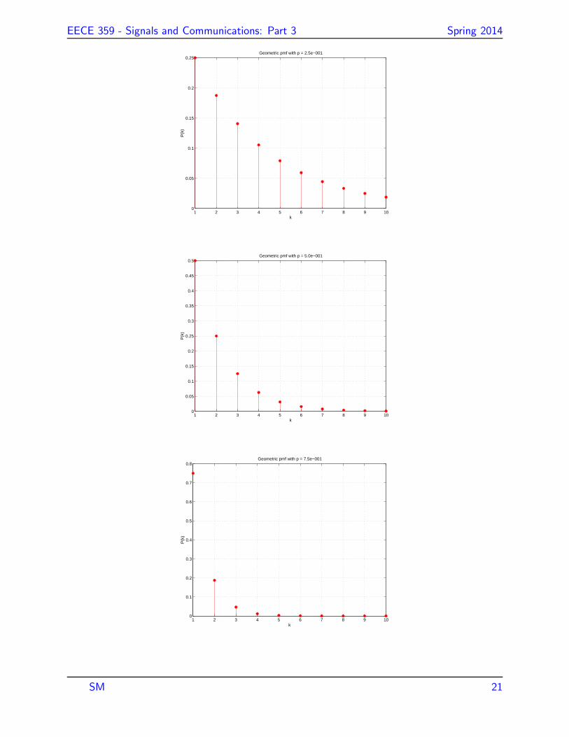
Example: Geometric distribution

Consider the transmission of a data packet

over a communication channel. If the

packet is not received successfully, the

sender retransmits the packet. This process

is repeated until the packet is received

successfully.

Suppose that packet errors are independent

and the probability that the packet is

successfully received on any transmission or

retransmission is p. Let X be the number of

transmissions required. Then,

P (X = k) = (1− p)k−1p, k = 1, 2, . . . (23)

Any rv with pmf given by (23) is referred to

as a geometric rv with parameter p.

The geometric pmf is plotted below for p =

0.25, 0.5 and 0.75.

SM 20


1 2 3 4 5 6 7 8 9 100

0.05

0.1

0.15

0.2

0.25Geometric pmf with p = 2.5e−001

k

P(k

)

1 2 3 4 5 6 7 8 9 100

0.05

0.1

0.15

0.2

0.25

0.3

0.35

0.4

0.45


k

P(k

)

1 2 3 4 5 6 7 8 9 100

0.1

0.2

0.3

0.4

0.5

0.6

0.7


k

P(k

)

SM 21


Continuous random variables

A continuous rv is one which takes on

a continuum of values and is commonly

described by its probability density function

(pdf) or its cumulative distribution function

(CDF).

Example: Uniform distribution

The rv X is said to be uniformly distributed

over the interval (a, b), denoted by U(0, 1), if

its pdf is given by

fX(x) =

{

1b−a, a < x < b

0, otherwise.(24)

xa

1/(b-a)

b

f(x)

SM 22


The uniform distribution is commonly used to

model quantization noise. We will also see

how it can be used to generate samples of

rv’s with arbitrary distributions.

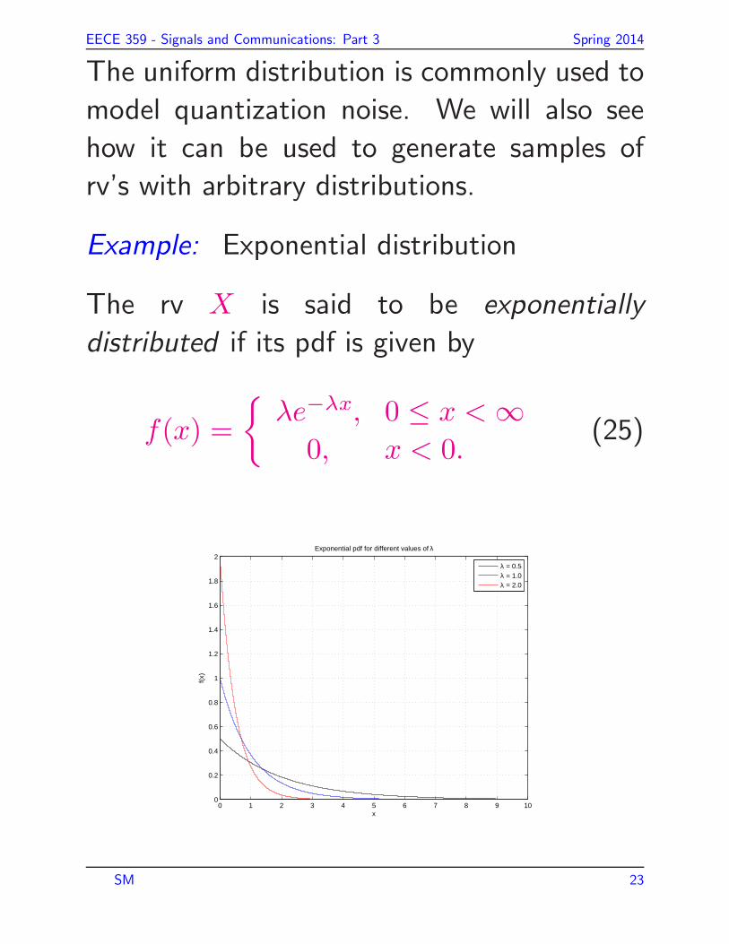
Example: Exponential distribution

The rv X is said to be exponentially

distributed if its pdf is given by

f(x) =

{

λe−λx, 0 ≤ x < ∞0, x < 0.

(25)

0 1 2 3 4 5 6 7 8 9 100

0.2

0.4

0.6

0.8

1

1.2

1.4

1.6

1.8

2Exponential pdf for different values of λ

x

f(x)

λ = 0.5λ = 1.0λ = 2.0

SM 23


From (25), the CDF of the exponential

distribution is

F (x) =

{

1− e−λx, 0 ≤ x < ∞0, x < 0.

(26)

The exponential distribution is commonly

used to model the time between adjacent

arrivals (also referred to as the inter-arrival

time) in a queueing system; in this case,

the parameter λ represents the arrival rate of

customers to the system.

The exponential distribution has an

interesting memoryless property. It can be

shown that

Pr{X ≤ x+ x0|X > x0}

=

{

1− e−λx, 0 ≤ x < ∞0, x < 0.

(27)

SM 24


Example: Gaussian or normal distribution

The Gaussian distribution, denoted by

N (µ, σ2), is one of the most important

distributions used in the analyses of

communication problems. Its pdf is given

by

f(x) =1√2πσ

e−(x−µ)2/2σ2,−∞ < x < ∞(28)

where µ is the mean, σ2 is the variance and

σ is the standard deviation.

−5 −4 −3 −2 −1 0 1 2 3 4 50

0.1

0.2

0.3

0.4

0.5

0.6

0.7zero mean Gaussian pdfs with variances σ2 = 0.5, 1, 2.0

x

f(x)

σ2 = 0.5

σ2 = 1.0

σ2 = 2.0

SM 25


Important functions in error analyses:

The erfc(.) and Q(.) functions are defined

as:

erfc(α)∆=

2√π

∫ ∞

α

e−x2 dx (29)

Q(α)∆=

1√2π

∫ ∞

α

e−x2

2 dx (30)

The Q(.) function is the area under the “tail”

of a zero mean, unit variance Gaussian pdf.

−5 −4 −3 −2 −1 0 1 2 3 4 50

0.05

0.1

0.15

0.2

0.25

0.3

0.35

0.4zero mean, unit variance Gaussian pdf

x

pdf

SM 26


Fact:

Q(x) =1

2erfc

(

x√2

)

(31)

In general, the values of these functions have

to be obtained numerically or looked up in

tables. Corresponding MATLAB functions

are erfc and qfunc.

Useful bounds for Q(.):

1√2πx

e−x2/2

(

1− 1

x2

)

< Q(x) <1√2πx

e−x2/2 (32)

0 0.5 1 1.5 2 2.5 3 3.5 4 4.5 510

−7

10−6

10−5

10−4

10−3

10−2

10−1

100

101

102

Q function and bounds

x

SM 27


Fact: Suppose the random variable (rv) X is

Gaussian with mean µ and variance σ2, i.e.

X ∼ N (µ, σ2). Then

P (X ≥ a) = Q

(

a− µ

σ

)

(33)

Proof:

Note: By symmetry,

P (X ≤ a) = P (X ≥ 2µ− a)

= Q

(

µ− a

σ

)

(34)

SM 28


Example: What is the probability that the

rv X ∼ N (µ, σ2) deviates from its mean, µ,

by more than cσ, i.e. Pr{|X − µ| > cσ}?

Solution:

Some numerical values

c 2Q(c)

0.5 0.617

1 0.317

2 4.55× 10−2

3 2.70× 10−3

4 6.33× 10−5

SM 29


From the table, we can say that in a

population of Gaussian distributed values,

about 95.5% of the values will be within two

standard deviations of the mean value.

The Q(.) function arises frequently in error

analyses when an additive white Gaussian

noise (AWGN) channel is assumed.

Suppose that the received signal in a certain

binary communication system is

r = s+ n (35)

where the transmitted signal, s, takes on

value +1 or −1 with equal probability of 12

and n is a sample value drawn from a Gaussian

distribution with zero mean and variance σ2.

We can view s as being sent over an additive

Gaussian noise channel.

Then, the conditional probability of error,

SM 30


given either +1 or −1 is sent, can be easily

obtained in terms of the Q(.) function.

Here is how

What should the decision threshold, T , be set

to?

If T is set to 0, then by symmetry, the

probability of error, Pe, is the same whether

+1 or −1 is sent. Assuming −1 is sent, we

have

Pe|s=−1 = Pr{R > 0}

= Q

(

0− (−1)

σ

)

= Q

(

1

σ

)

. (36)

SM 31


Averages and moments

We are often interested in evaluating the

average value of a rv X or some function

of the rv.

Defn: Suppose that Y = h(X). The

expected value, expectation or ensemble

average of Y is

E[Y ] = Y =

∫ ∞

−∞h(x)fX(x)dx (37)

For a discrete rv X, from (37), the expected

value can be evaluated as

E[Y ] = Y =M∑

i=1

h(xi)p(xi) (38)

where M is the number of possible values of

X.

Remark: The expectation operator is linear,

SM 32


i.e.

E[ah1(X) + bh2(X)] = aE[h1(X)] + bE[h2(X)] (39)

Notation: The expected value, E[X], of a rv

X is commonly called its mean and denoted

by mX. It gives the “center of mass” of the

distribution.

Exercise: Determine the expected value of

the uniform distribution in (24).

Solution: From (37), we have

E[X] = X =

∫ b

a

x1

b− adx

=1

b− a

[

x2

2

]b

a

=a+ b

2

Exercise: Show that

SM 33


1. the mean of the exponential distribution in

(25) is 1λ

2. the mean of the Gaussian distribution in

(28) is µ

3. the mean of the Binomial distribution in

(19) is nε

4. the mean of the Poisson distribution in (22)

is λ

5. the mean of the geometric distribution in

(23) is 1p

Other common measures of a distribution:

• the median is the value, x, of X at which

P (X > x) = P (X < x) (40)

SM 34


• the mode is the value, x, of X at which

fX(x) is maximum.

Moments

Moments are defined as the expected values

of specific functions of X.

Defn: The rth moment of X, denoted by µr,

is

E[Xr]∆=

∫ ∞

−∞xrfX(x) dx (41)

Remark: µ1 is the mean value and µ2 is the

mean square value of X.

Defn: The rth central moment ofX, denotedby µ′

r, is

E[(X −mX)r]∆=

∫ ∞

−∞(x−mX)rfX(x) dx (42)

Remark: The second central moment, µ′2,

is called the variance of X, and is denoted

SM 35


by σ2X; σX is termed the standard deviation

and is commonly used as a measure of the

dispersion of X.

Fact:

σ2X = E[X2]−m2

X (43)

Proof:

Exercise: Determine the variance of the

uniform distribution in (24).

SM 36


Solution: From (41), we have

E[X2] =

∫ b

a

x2 1

b− adx

=1

b− a

[

x3

3

]b

a

=a2 + ab+ b2

3

Using (43), we have

var(X) = σ2X = E[X2]− (E[X])2

=a2 + ab+ b2

3−

(

a+ b

2

)2

=(b− a)2

12

Exercise: Show that

1. the variance of the exponential distribution

SM 37


in (25) is 1λ2

2. the variance of the Gaussian distribution in

(28) is σ2

3. the variance of the Binomial distribution in

(19) is nε(1− ε)

4. the variance of the Poisson distribution in

(22) is λ

5. the variance of the geometric distribution

in (23) is 1−pp2

SM 38


Generating samples of a random variable

with an arbitrary probability distribution

Random number generators (RNGs) are

commonly used in computer simulations to

assess the performance of communication

systems. For example, MATLAB provides

rand (randn) for generating samples drawn

from U(0, 1) (N (0, 1)) distributions. (See

below)

>> help randRAND Uniformly distributed pseudorandom numbers.R = RAND(N) returns an N-by-N matrix containingpseudorandom values drawn from the standard uniformdistribution on the open interval(0,1).

>> help randnRANDN Normally distributed pseudorandom numbers.R = RANDN(N) returns an N-by-N matrix containingpseudorandom values drawn from the standard normaldistribution.

How can we generate samples, x1, x2, x3, . . .,

from an arbitrary distribution with CDF

SM 39


FX(x)?

�� = ��(��)

��

0

��(�)

�

1

Step 1: Generate independent samples of

U(0, 1); call them ui, i = 1, 2, . . .

Step 2: Let xi = F−1X (ui), as shown in the

above figure. Then, the values xi, i = 1, 2, . . .

are drawn from the desired distribution.

Why?

We can check the distribution from which the

SM 40


values xi, i = 1, 2, . . . are drawn as follows.

FXi(x)

∆= P (Xi ≤ x)

= P (F−1X (Ui) ≤ x)

= P (Ui ≤ FX(x))

= FX(x) (44)

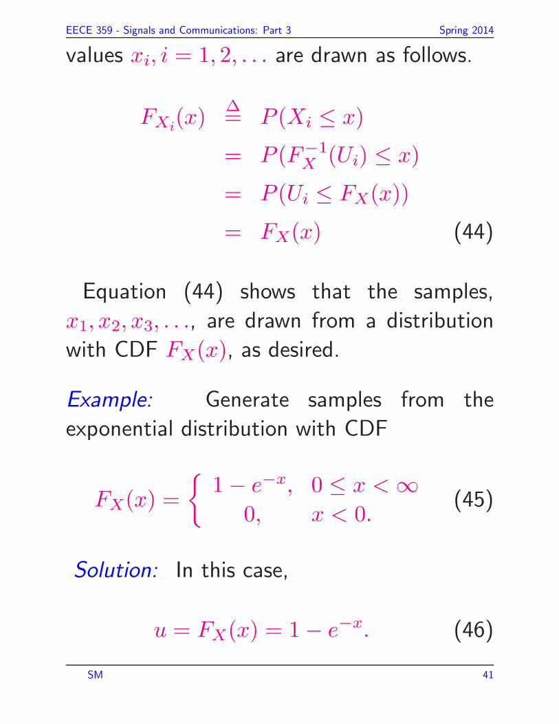
Equation (44) shows that the samples,

x1, x2, x3, . . ., are drawn from a distribution

with CDF FX(x), as desired.

Example: Generate samples from the

exponential distribution with CDF

FX(x) =

{

1− e−x, 0 ≤ x < ∞0, x < 0.

(45)

Solution: In this case,

u = FX(x) = 1− e−x. (46)

SM 41


Hence,

x = − ln(1− u). (47)

So, we first generate U(0, 1) samples

{ui, i = 1, 2, . . .}.

Then, the values {xi = − ln(1− ui), i = 1, 2, . . .}are samples from the desired exponential

distribution.

SM 42


Functional transformation of random

variables

� � = �(�)

�(�)

In the above figure, assume that the output

y = g(x) at any time instant depends only

on the input x at that time instant, i.e. the

system is memoryless.

Then, the pdf, fY (y), of the output, Y , can

be written in terms of the pdf, fX(x), of the

input, X as follows:

Theorem (Couch, p. 704)

fY (y) =M∑

i=1

fX(x)

|dy/dx|

∣

∣

∣

∣

x=xi

(48)

where x1, x2, . . . , xM are the M values of x

for which g(x) = y, |.| denotes the absolute

SM 43


value and the last vertical line denotes the

evaluation at x = xi.

Example: Rayleigh fading is commonly used

to model the amplitude of a signal transmitted

over a wireless communication channel. The

pdf of the channel amplitude gain follows a

Rayleigh distribution, i.e.

fA(a) =

{

2ab e−a2/b, a ≥ 0

0, a < 0.(49)

The channel power gain, Γ, is the square of

the channel amplitude gain, A. We wish to

determine the pdf, fΓ(γ), of Γ.

Using (48), with y = γ, x = a, and dγda = 2a,

we have

fΓ(γ) =fA(a)

2a

∣

∣

∣

∣

a=+√γ

+fA(a)

2a

∣

∣

∣

∣

a=−√γ

(50)

Note that the second term on the RHS of

SM 44


(50) is 0, since fA(a) = 0, a < 0. Therefore,

fΓ(γ) =

{

1b e−γ/b, γ ≥ 0

0, γ < 0.(51)

Equation (51) is the exponential pdf with

mean b. We conclude that the pdf of

the square of a Rayleigh distributed rv is

exponential.

The two pdfs are plotted in the figure below,

with b = 4/π which corresponds to a unity

mean for the Rayleigh distribution.

0 1 2 3 4 5 60

0.1

0.2

0.3

0.4

0.5

0.6

0.7

0.8Rayleigh and Exponential pdfs for b=4/pi

x

f(x)

Rayleigh Exponential

SM 45


Multivariate statistics

So far, we have looked at pdfs and CDFs of

one rv. These can be extended to the case of

N > 1 rv’s. For simplicity, we focus on the

N = 2, i.e. bivariate case.

Defn: The 2-dimensional cumulative

distribution function (CDF) of the rv’s X

and Y is

FX,Y (x, y) = P (X ≤ x and Y ≤ y) (52)

Defn: The 2-dimensional probability density

function (pdf) of the rv’s X and Y is

fX,Y (x0, y0) =∂2FX,Y (x, y)

∂x∂y

∣

∣

∣

∣

(x,y)=(x0,y0)

(53)

Properties of 2-D CDFs

• FX,Y (x, y) is a non-decreasing function of

x and y.

SM 46


• FX,Y (−∞,−∞) = 0

• FX,Y (∞,∞) = 1

Note that FX,Y (x,∞) = FX(x).

Properties of 2-D pdf’s

• f(x, y) is a non-negative function, i.e.

f(x, y) ≥ 0.

•∫ ∞

−∞

∫ ∞

−∞f(x, y)dxdy = 1. (54)

• f(x, y) = f(x)f(y|x).

Defn: The expected value of g(X,Y ) is

E[g(X,Y )] =

∫ ∞

−∞

∫ ∞

−∞g(x, y)fX,Y (x, y)dxdy (55)

SM 47


Defn: Two rv’s X and Y are independent if

fX,Y (x, y) = fX(x)fY (y). (56)

Defn: The correlation of X and Y is

E[XY ] =

∫ ∞

−∞

∫ ∞

−∞xyfX,Y (x, y)dxdy. (57)

Defn: Two rv’s X and Y are uncorrelated if

E[XY ] = E[X]E[Y ]. (58)

Defn: The covariance of X and Y is

Cov(X,Y ) = E[(X − mX)(Y − mY )] (59)

=

∫ ∞

−∞

∫ ∞

−∞(x − mX)(y − mY )fX,Y (x, y)dxdy. (60)

Exercise: Show that

• Cov(X, Y ) = E[XY ]− E[X ]E[Y ]

SM 48


• Var(X + Y ) = Var(X) + Var(Y ) + 2 Cov(X, Y )

Defn: The correlation coefficient (also called

the normalized covariance) of X and Y is

ρ =Cov(X,Y )

σXσY. (61)

Facts:

• −1 ≤ ρ ≤ +1.

• If X and Y are independent, then they

are also uncorrelated. The converse is not

generally true. However, the converse is

true for bivariate Gaussian rv’s (See Couch,

p. 712, for the pdf).

• If X and Y are independent, then their

covariance is zero. The converse is not

generally true. However, the converse is

true for jointly Gaussian rv’s.

SM 49


• The pdf of the sum of independent rv’s is

given by the convolution of the individual

pdf’s.

Exercise: Determine the pdf of the sum of

two independent U(0, 1) rv’s.

• Central Limit Theorem (CLT) The CDF of

a sum of N independent rv’s approaches a

Gaussian CDF as N increases.

• Chebyshev’s Inequality If X is a rv with

finite mean µ and variance σ2, then for any

k > 0,

P (|X − µ| ≥ kσ) ≤ 1

k2(62)

Exercise: Let Xn be the number of headsin n tosses of a fair coin and Yn = Xn/n.Show that

P (|Yn − 0.5| ≥ ε) ≤ 1

4nε2(63)

SM 50

notes part 3 - UBCcourses.ece.ubc.ca/359/notes/notes_part3.pdfEECE 359 - Signals and Communications:...

Documents

Transcript of notes part 3 - UBCcourses.ece.ubc.ca/359/notes/notes_part3.pdfEECE 359 - Signals and Communications:...