notes part 1 - University of British Columbiacourses.ece.ubc.ca/359/notes/notes_part1.pdf ·...
77
EECE 359 - Signals and Communications: Part 1 Spring 2014 Introduction 1 Signals are generated by a wide variety of sources and contain information about the behaviour or nature of the source. Example signals are text, speech, music, video, sensor data, stock market index value, etc. Often we are interested in processing signals to extract information of interest. In general, systems process signals and produce other signals. Example of processed signals are equalized or distorted music! Communication channel Source Transmitter Sink Receiver Simplified block diagram of a communication system The purpose of a communication system is to convey messages (information) from a source 1 These slides are based on lecture notes of Professors L. Lampe, C. Leung, and R. Schober SM 1
Transcript of notes part 1 - University of British Columbiacourses.ece.ubc.ca/359/notes/notes_part1.pdf ·...

EECE 359 - Signals and Communications: Part 1 Spring 2014
Introduction1
Signals are generated by a wide variety of
sources and contain information about the
behaviour or nature of the source. Example
signals are text, speech, music, video, sensor
data, stock market index value, etc. Often we
are interested in processing signals to extract
information of interest. In general, systems
process signals and produce other signals.
Example of processed signals are equalized
or distorted music!
Communication
channel Source Transmitter
Sink Receiver
Simplified block diagram of a communication system
The purpose of a communication system is to
convey messages (information) from a source1These slides are based on lecture notes of Professors L.
Lampe, C. Leung, and R. Schober
SM 1

EECE 359 - Signals and Communications: Part 1 Spring 2014
to a destination (sink). Examples of sources
and sinks: person, computer, memory, etc.
Communication is typically done using signals
that are carefully designed to result in
an efficient and cost-effective information
transfer.
The medium through which the signals are
sent is referred to as channel and can
cause distortion and introduce other types
of impairments, e.g. noise, fading.
A high level perspective
Common communication channels are
inherently analog in nature, e.g., telephone
wires, coaxial cable, optical fiber, infrared,
cellular, satellite, and power line channels.
Why are digital communication systems
preferred over their analog counterparts?
SM 2

EECE 359 - Signals and Communications: Part 1 Spring 2014
Many trade-offs are involved in the design of
digital communication systems. The designer
tries to minimize the cost while meeting all
performance specifications.
System considerations include: cost,
bandwidth, data rate, power consumption,
security delay, error performance, and
subjective quality.
To send information digitally, we often need
to convert analog signals to digital form.
How can we do this?
Use sampling and quantization.
• How often should we sample?
• How finely should we quantize?
SM 3

EECE 359 - Signals and Communications: Part 1 Spring 2014
Example: Compact Disc (CD) system
Each one of the left and right channels is
sampled at a rate of 44,100 times per second.
Why this sampling rate?
We will later discuss Sampling Theorem which
will shed light on the answer.
Typically, each of the samples is converted
into digital form using a 16-bit analog-to-
digital (A/D) converter or ADC.
This results in a 1.41 Mbps data stream.
A coding technique (in this case, CIRC or
cross-interleaved Reed-Solomon code) is used
to encode this 1,411,200 bps data stream
which results in a 1.88 Mbps encoded stream.
Such coding allows for error correction.
SM 4

EECE 359 - Signals and Communications: Part 1 Spring 2014
Typical digital data rate requirements:
Single-page fax 10 – 50 kB8 x 10 inch color image 1 – 8 MBVoice 8 – 32 kbpsAudio (MP3) 32 – 384 kbpsVideo (H.261 conferencing) 64 kbps – 1.5 MbpsHD Video (MPEG-2, MPEG-4) 2 – 50 Mbps
SM 5

EECE 359 - Signals and Communications: Part 1 Spring 2014
Important events in development of communicationsystems
1838 Telegraph (Cooke and Wheatstone)1871 Telephone “Caveat” Some believe Antonio
Meucci (not A.G. Bell) was the inventor ofthe talking telegraph or telephone.
1900 Marconi sends wireless signal across Atlantic.1920 Beginning of radio broadcasting.1936 First public B/W TV broadcast.1951 First public color TV broadcast.1957 First earth satellite, Sputnik I.1962 First communication satellite, Telstar I.1966 Principles of fibre optic communications
published (Kao and Hockham).1973 Birth of Internet.1979 First-generation cellular phone service.1985 Fax machines gain popularity.1990’s HDTV, second-generation cellular systems.2000’s Third-generation cellular systems, satellite
radio, “anytime, anywhere, multimediacommunications”.
2010’s Online social networks, smart phones, LTE,wireless sensor networks (WSNs).
Note the increasingly rapid pace of innovations.
SM 6

EECE 359 - Signals and Communications: Part 1 Spring 2014
Continuous-time (CT) and discrete-time
(DT) signals – Section 1.1
Notation
CT: x(t), y(t), or other functions of a
variable t where t is a real-valued independent
variable; t often but not always refers to time;
e.g., it could be a spatial variable.
DT: x[n], y[n], or other functions of a variable
n where n is an integer-valued independent
variable. A DT signal is not defined for non-
integer values of n.
A DT signal may result from a source that
is inherently discrete time, e.g., daily closing
index of the TSE; it may also result from the
sampling of a CT signal.
SM 7
EECE 359 - Signals and Communications: Part 1 Spring 2014
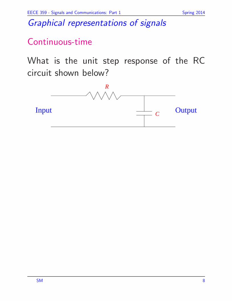
Graphical representations of signals
Continuous-time
What is the unit step response of the RC
circuit shown below?
Input Output
R
C
SM 8

EECE 359 - Signals and Communications: Part 1 Spring 2014
Discrete-time
Signal energy and power
CT: The total energy in a possibly complex-
valued signal x(t) over the time interval
t1 ≤ t ≤ t2 is defined as
E∆=
∫ t2
t1
|x(t)|2 dt
where |x(t)| denotes the magnitude of x(t).
SM 9

EECE 359 - Signals and Communications: Part 1 Spring 2014
The average power is defined as
P∆=
E
t2 − t1.
Example: Determine the total energy and
average power of the signal x(t) = 1 − e−t
over the time interval (0, 5).
SM 10
EECE 359 - Signals and Communications: Part 1 Spring 2014
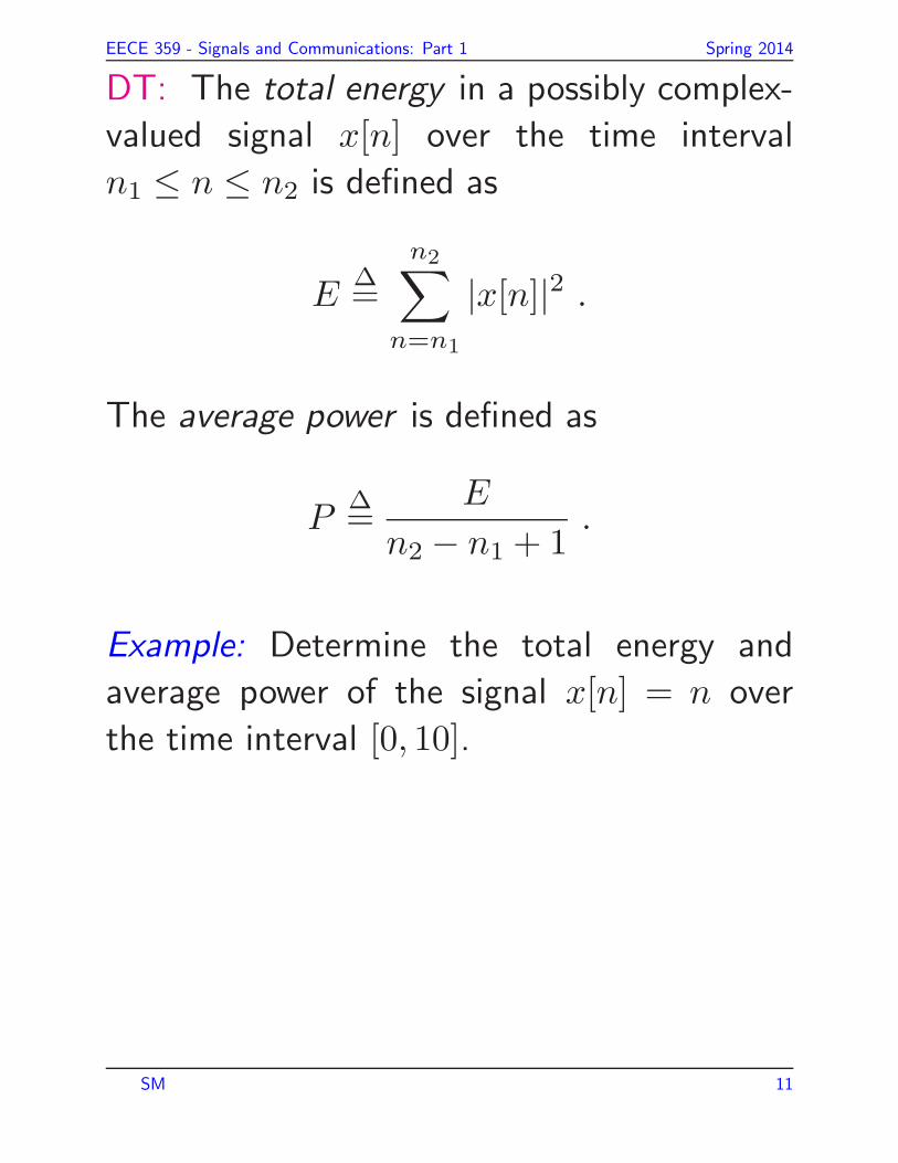
DT: The total energy in a possibly complex-
valued signal x[n] over the time interval
n1 ≤ n ≤ n2 is defined as
E∆=
n2∑
n=n1
|x[n]|2 .
The average power is defined as
P∆=
E
n2 − n1 + 1.
Example: Determine the total energy and
average power of the signal x[n] = n over
the time interval [0, 10].
SM 11

EECE 359 - Signals and Communications: Part 1 Spring 2014
Question: How do we define the total energy
and average power for signals over an infinitely
long time interval?
Answer: By taking limits in the above
definitions.
CT:
E∞∆= lim
T→∞
∫ T
−T
|x(t)|2 dt
P∞∆= lim
T→∞
1
2T
∫ T
−T
|x(t)|2 dt .
DT:
E∞∆= lim
N→∞
N∑
n=−N
|x[n]|2
P∞∆= lim
N→∞
1
2N + 1
N∑
n=−N
|x[n]|2 .
SM 12

EECE 359 - Signals and Communications: Part 1 Spring 2014
Classification of signals
1. Finite total energy, i.e., E∞ < ∞ . This
implies that P∞ = 0.
2. Finite average power, i.e., 0 < P∞ < ∞ .
This implies that E∞ = ∞ .
3. Infinite average power, i.e., P∞ = ∞ . For
example, x[n] = n,−∞ < n < ∞ .
Transformation of the independent
variable – Section 1.2
Consider the signal shown in below.
t
x(t)
1
101–
A sample signal x(t)
SM 13

EECE 359 - Signals and Communications: Part 1 Spring 2014
Let us sketch the signals obtained when we
change the independent variable as follows.
t
x(−t)
1
101–2– 2
t
x(t−1)
1
101–2– 2
t
x(2t)
1
101–2– 2
SM 14

EECE 359 - Signals and Communications: Part 1 Spring 2014
t
x(2t−1)
1
101–2– 2
More generally, to obtain x(αt − β), we first
delay x(t) by β and then perform the time
scaling/reversal by α.
Equivalently, to obtain x(
α[
t− βα
])
, we first
time scale/reverse by α and then delay by βα.
Periodic signals – Section 1.2.2
CT: x(t) is periodic with period T > 0 if
x(t+ T ) = x(t) for all values of t .
The smallest value of T for which this holds
is called the fundamental period, T0.
SM 15

EECE 359 - Signals and Communications: Part 1 Spring 2014
Example: cosω0t is periodic with
fundamental period T0 =2πω0
.
This signal is related to the CT complex
exponential signal, ejω0t, via Euler’s formula
ejθ = cos θ + j sin θ .
DT: x[n] is periodic with period N > 0 if
x[n+N ] = x[n] for all values of n .
The smallest value of N for which this holds
is called the fundamental period, N0.
Example: DT complex exponential signal,
ejω0n .
Note: There are important differences
between the CT and DT complex exponential
signals.
SM 16
EECE 359 - Signals and Communications: Part 1 Spring 2014
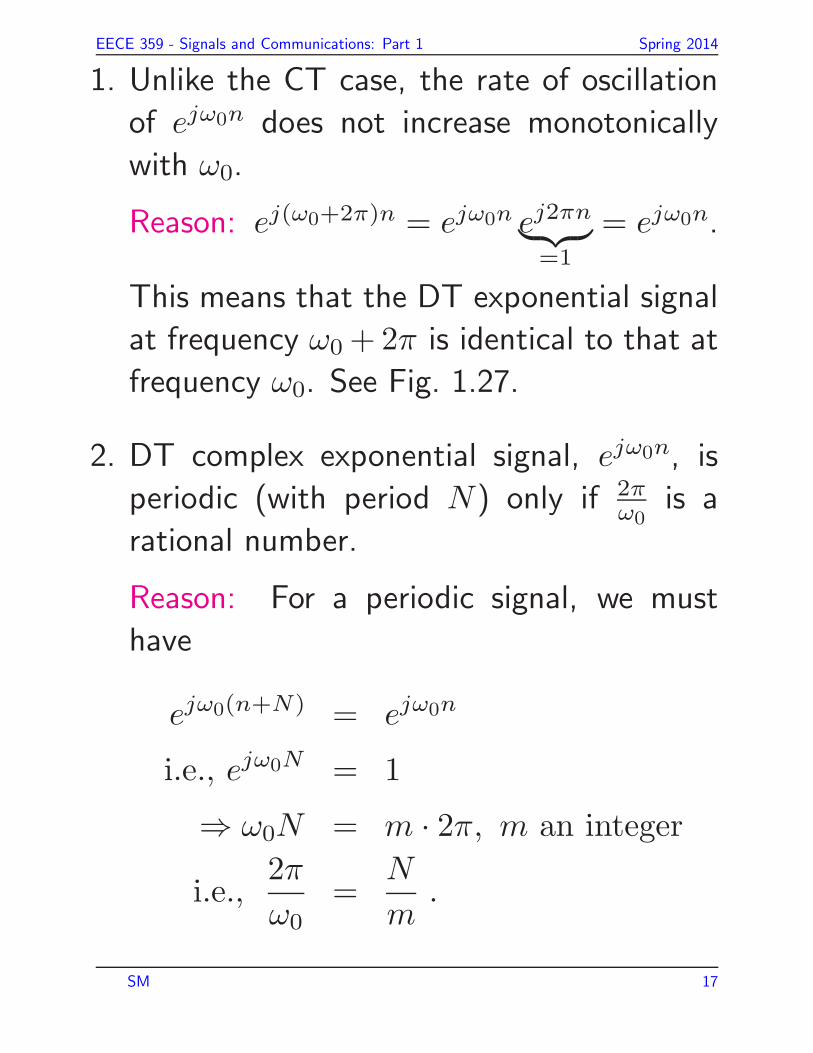
1. Unlike the CT case, the rate of oscillation
of ejω0n does not increase monotonically
with ω0.
Reason: ej(ω0+2π)n = ejω0n ej2πn︸ ︷︷ ︸=1
= ejω0n.
This means that the DT exponential signal
at frequency ω0+2π is identical to that at
frequency ω0. See Fig. 1.27.
2. DT complex exponential signal, ejω0n, is
periodic (with period N) only if 2πω0
is a
rational number.
Reason: For a periodic signal, we must
have
ejω0(n+N) = ejω0n
i.e., ejω0N = 1
⇒ ω0N = m · 2π, m an integer
i.e.,2π
ω0=
N
m.
SM 17

EECE 359 - Signals and Communications: Part 1 Spring 2014
Demystifying Figure 1.27 of textbook
Observations:
1. Slowly-varying (low-frequency) DT sinusoidal
sequences have ω0 close to 0,±2π,±4π, . . .;
Rapidly-varying (high-frequency) DT sinusoidal
sequences have ω0 close to ±π,±3π, . . .
2. The sequences cos(π−θ)n and cos(π+θ)n
are identical, e.g., Fig. 1.27(c) and (g)
correspond to θ values of 3π/4.
Analytic proof of the second observation
Recall that
cos(α+ β) = cosα cosβ − sinα sin β
cos(α− β) = cosα cosβ + sinα sin β.
SM 18

EECE 359 - Signals and Communications: Part 1 Spring 2014
Thus,
cos(π − θ)n = cos(πn− θn)
= cosπn cos θn+ sinπn sin θn
= (−1)n cos θn.
Similarly,
cos(π + θ)n = cos(πn+ θn)
= cosπn cos θn− sinπn sin θn
= (−1)n cos θn.
A graphical viewpoint
0 1 2 3 4 5 6 7 8 9 10
−1
−0.5
0
0.5
1
t (seconds)
cos (0*pi*t) cos (0.5*pi*t)cos (pi*t) cos (1.5*pi*t)cos (2*pi*t)
SM 19

EECE 359 - Signals and Communications: Part 1 Spring 2014
Even and odd signals
Defn: A signal x(t) or x[n] is said to be even
if
CT : x(−t) = x(t)
DT : x[−n] = x[n].
Defn: A signal x(t) or x[n] is said to be odd
if
CT : x(−t) = −x(t)
DT : x[−n] = −x[n].
Examples
x(t) = t2 is even, as is x[n] = n2.
x(t) = t3 is odd, as is x[n] = n3.
x(t) = t+ 1 is neither even nor odd.
SM 20

EECE 359 - Signals and Communications: Part 1 Spring 2014
Facts
1. A function which is both even and odd has
to be equal to 0.
2. The sum of two even functions is even.
3. The sum of two odd functions is odd.
4. Any signal x(t) (or x[n]) can be written in
a unique way as the sum of an even signal
and an odd signal, i.e.,
x(t) = xe(t) + xo(t)
where the even part is given by
xe(t) =1
2[x(t) + x(−t)]
and the odd part is given by
xo(t) =1
2[x(t)− x(−t)].
SM 21
EECE 359 - Signals and Communications: Part 1 Spring 2014
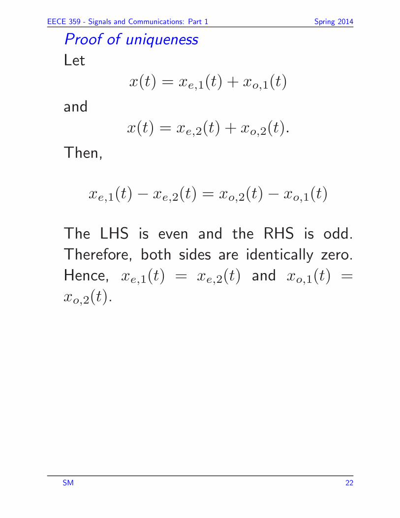
Proof of uniqueness
Let
x(t) = xe,1(t) + xo,1(t)
and
x(t) = xe,2(t) + xo,2(t).
Then,
xe,1(t)− xe,2(t) = xo,2(t)− xo,1(t)
The LHS is even and the RHS is odd.
Therefore, both sides are identically zero.
Hence, xe,1(t) = xe,2(t) and xo,1(t) =
xo,2(t).
SM 22

EECE 359 - Signals and Communications: Part 1 Spring 2014
Two important signals: Unit impulse and
unit step functions – Section 1.4
Discrete-Time:
Unit impulse or unit sample
δ[n] =
{0, n 6= 0
1, n = 0.
n
1
10
1–3– 2
δ n[ ]
32–
Unit step sequence
u[n] =
{0, n < 0
1, n ≥ 0.
n
1
10
1–3– 2
u n[ ]
32–
SM 23
EECE 359 - Signals and Communications: Part 1 Spring 2014
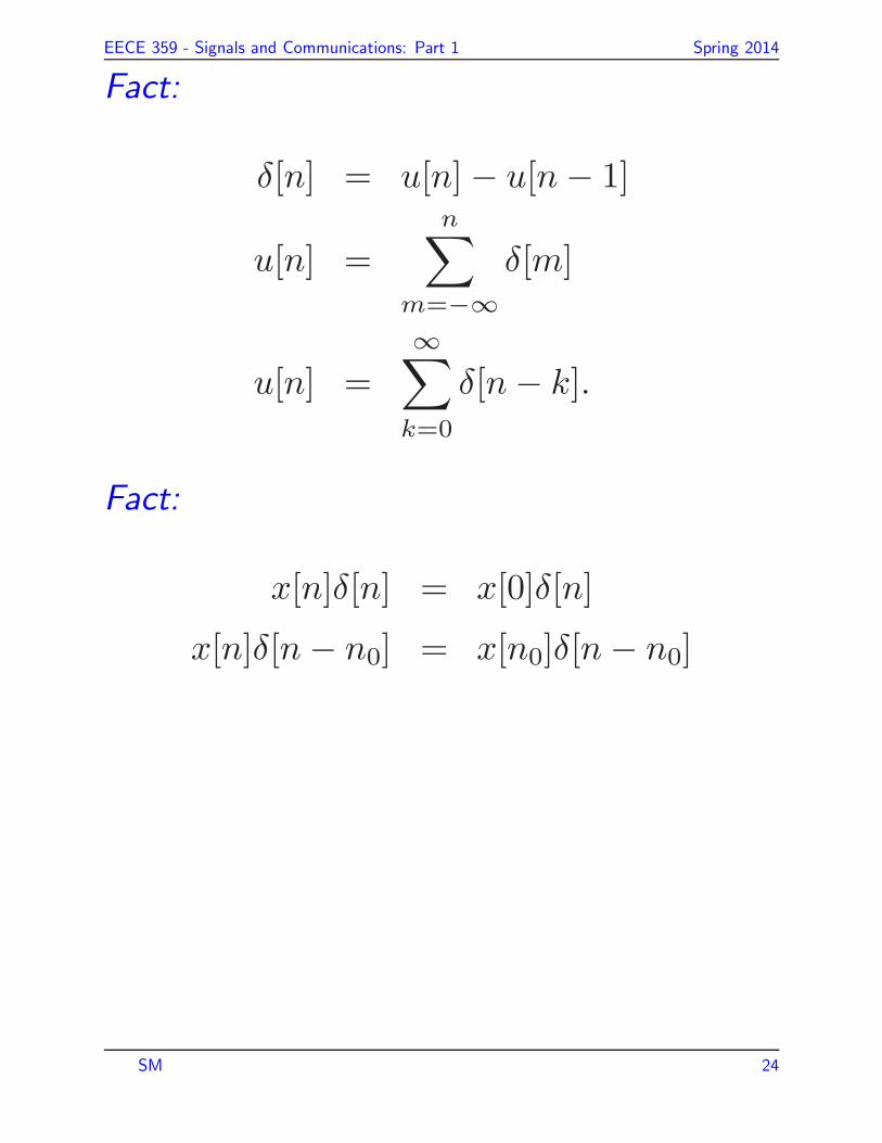
Fact:
δ[n] = u[n]− u[n− 1]
u[n] =n∑
m=−∞
δ[m]
u[n] =
∞∑
k=0
δ[n− k].
Fact:
x[n]δ[n] = x[0]δ[n]
x[n]δ[n− n0] = x[n0]δ[n− n0]
SM 24
EECE 359 - Signals and Communications: Part 1 Spring 2014
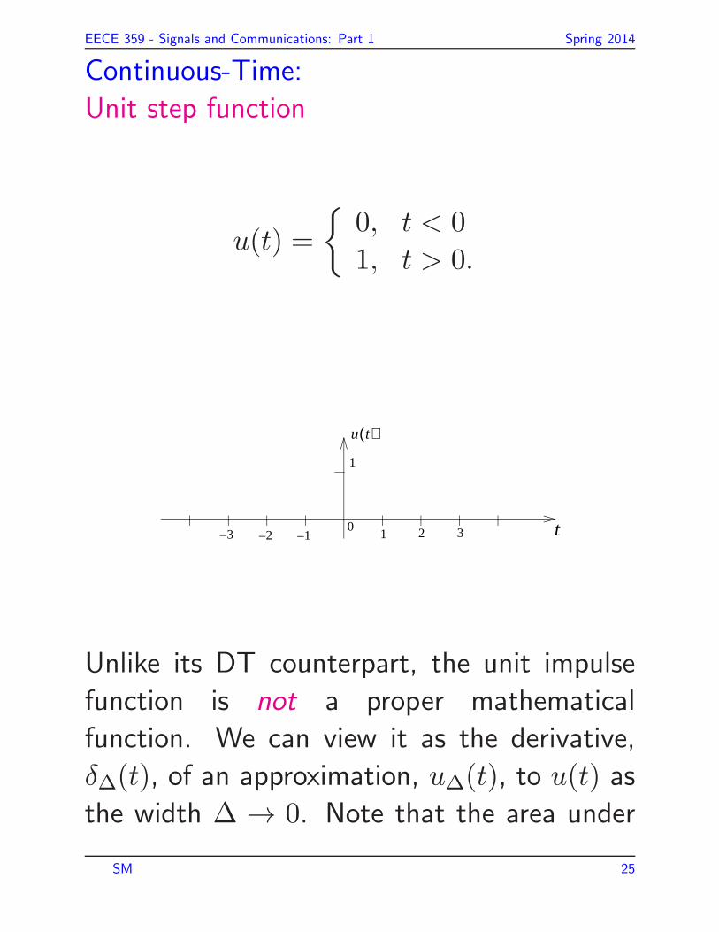
Continuous-Time:
Unit step function
u(t) =
{0, t < 0
1, t > 0.
t
1
10
1–3– 2
u t( )
32–
Unlike its DT counterpart, the unit impulse
function is not a proper mathematical
function. We can view it as the derivative,
δ∆(t), of an approximation, u∆(t), to u(t) as
the width ∆ → 0. Note that the area under
SM 25

EECE 359 - Signals and Communications: Part 1 Spring 2014
δ∆(t) is constant and is equal 1.
t
1
0
u∆ t( )
∆
t
1∆---
0
δ∆ t( )
∆
t
1
0
δ t( ) δ∆ t( )∆ 0→lim=
Sampling property of δ(t): For a “smooth”
function x(t),
x(t)δ(t− t0) = x(t0)δ(t− t0).
SM 26

EECE 359 - Signals and Communications: Part 1 Spring 2014
Continuous-time and discrete-time systems
– Section 1.5
CT systemx t( ) y t( )
Short-hand: x t( ) y t( )→
DT systemx n[ ] y n[ ]
Short-hand: x n[ ] y n[ ]→
Interconnection of systems
1. Series or cascade
2. Parallel
SM 27
EECE 359 - Signals and Communications: Part 1 Spring 2014
3. Hybrid – Series and parallel
4. Feedback
SM 28

EECE 359 - Signals and Communications: Part 1 Spring 2014
System properties – Section 1.61. Linearity
Defn (CT): If x1(t) → y1(t) and x2(t) →
y2(t), then for any constants a, b we have
ax1(t) + bx2(t) → ay1(t) + by2(t).
An important result: For a linear system,
a 0 input always results in a 0 output.
Example: System whose I/O relationship is
given by y(t) = tx(t).
SM 29

EECE 359 - Signals and Communications: Part 1 Spring 2014
Example: System whose I/O relationship is
given by y[n] = x2[n].
Example: System whose I/O relationship
is given by y[n] = 2x[n] + 1.
SM 30

EECE 359 - Signals and Communications: Part 1 Spring 2014
2. Time-invariance
Defn (DT): A system is time-invariant if
a time-shift in the input signal results in an
identical shift in the output signal, i.e.,
If x[n] → y[n], then x[n− n0] → y[n− n0].
A similar definition holds for CT systems.
Example: System whose I/O relationship is
given by y[n] = x2[n].
SM 31
EECE 359 - Signals and Communications: Part 1 Spring 2014
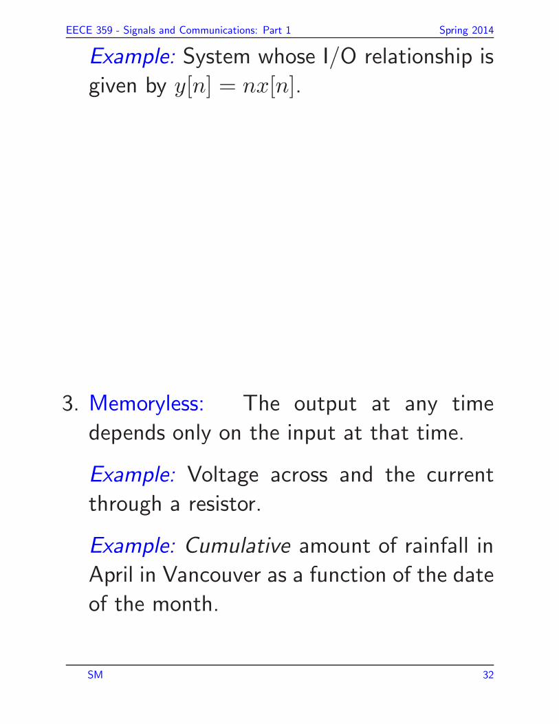
Example: System whose I/O relationship is
given by y[n] = nx[n].
3. Memoryless: The output at any time
depends only on the input at that time.
Example: Voltage across and the current
through a resistor.
Example: Cumulative amount of rainfall in
April in Vancouver as a function of the date
of the month.
SM 32

EECE 359 - Signals and Communications: Part 1 Spring 2014
4. Causal: The output at any time depends
only on the input values at that time or
previous times (system is non-anticipative).
Example: Any physical system in which the
independent variable is time.
Example:
y[n] =1
3{x[n− 1] + x[n] + x[n+ 1]}.
5. Stable If the input is finite, then the output
is also finite.
SM 33

EECE 359 - Signals and Communications: Part 1 Spring 2014
Example: In the RC circuit shown below,
the input is a voltage across the input
terminals and the output is the voltage
across the output terminals.
Input Output
R
C
Example: In the same RC circuit, the input
is a constant current and the output is the
voltage across the output terminals.
SM 34

EECE 359 - Signals and Communications: Part 1 Spring 2014
Linear time-invariant (LTI) systems –
Chapter 2
We will derive the output of DT LTI
systems. We will show that the input-output
relationship of such a system is completely
characterized by the unit impulse response of
the system.
Discrete-time LTI systems – Section 2.1
Convolution sum
Let h[n] denote the unit impulse (sample)
response of an LTI system, i.e.,
δ[n] → h[n].
Then, by the TI property,
δ[n− k] → h[n− k] (1)
We note that any signal x[n] can be written
SM 35

EECE 359 - Signals and Communications: Part 1 Spring 2014
as
x[n] =
∞∑
k=−∞
x[k]δ[n− k]. (2)
To explain why (2) is true, we consider the
following.
Example:
n
1
10
1–3– 2
x n[ ]
32–
2
3
For the signal in the above figure, we have
x[n] = δ[n+ 1] + 2δ[n] + 3δ[n− 1] + δ[n− 2]
which verifies (2).
Using (1) and the scaling property, we can
SM 36

EECE 359 - Signals and Communications: Part 1 Spring 2014
write
x[k]δ[n− k] → x[k]h[n− k].
Finally using the additive property , we have
∞∑
k=−∞
x[k]δ[n− k] →∞∑
k=−∞
x[k]h[n− k].
Note that h[n− k] is a time-reversed version
of h[k] delayed by n, i.e., if n is positive, we
shift the time-reversed version to the right.
x n[ ] y n[ ]LTIh n[ ]
The output in the above figure can be
expressed as
y[n] =
∞∑
k=−∞
x[k]h[n− k]
SM 37

EECE 359 - Signals and Communications: Part 1 Spring 2014
We say that y[n] is the convolution of x[n] and
h[n]; this relationship is commonly written as
y[n] = x[n] ∗ h[n].
Example:
n
1
10
1– 2
x n[ ]
32–
n
1
10
1– 2
h n[ ]
32–
We want to determine the output of the above
LTI system, i.e.,
y[n] = x[n] ∗ h[n].
SM 38

EECE 359 - Signals and Communications: Part 1 Spring 2014
k
1
10
1– 2
x k[ ]
32–
k
1
10
1– 2
h k[ ]
32–
k
1
10
1– 2
h k–[ ]
32–
k
1
10
1– 2
h n k–[ ]
n
2–
n 1–
SM 39

EECE 359 - Signals and Communications: Part 1 Spring 2014
n
1
10
1– 2
y n[ ]
32– 4 5
2
MATLABr is a high-level language and
environment for numerical computations
for variety of applications including signal
processing. It can be used to compute y[n].
A simple MATLABr script, convol.m, for
this purpose and the result of running the
script is shown below.
SM 40

EECE 359 - Signals and Communications: Part 1 Spring 2014
% convol.m
% Matlab script file to evaluate the % convolution of two signals
x=[1 1 1] % index of first element is 1
h=[1 1]
y=conv(x,h)
Result from running above MATLAB script
EDU» clear allEDU» convol
x =
1 1 1
h =
1 1
y =
1 2 2 1
SM 41
EECE 359 - Signals and Communications: Part 1 Spring 2014
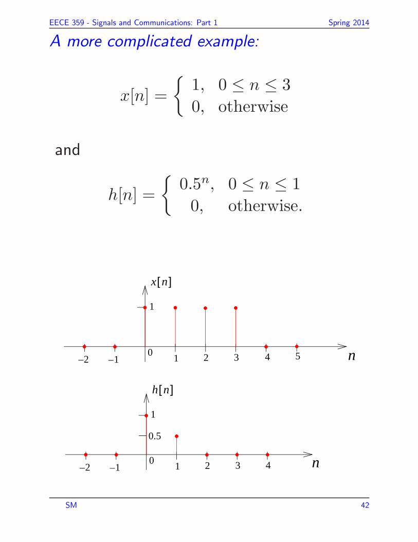
A more complicated example:
x[n] =
{1, 0 ≤ n ≤ 3
0, otherwise
and
h[n] =
{0.5n, 0 ≤ n ≤ 1
0, otherwise.
n
1
10
1– 2
x n[ ]
32–
n
1
10
1– 2
h n[ ]
32–
4 5
0.5
4
SM 42
EECE 359 - Signals and Communications: Part 1 Spring 2014
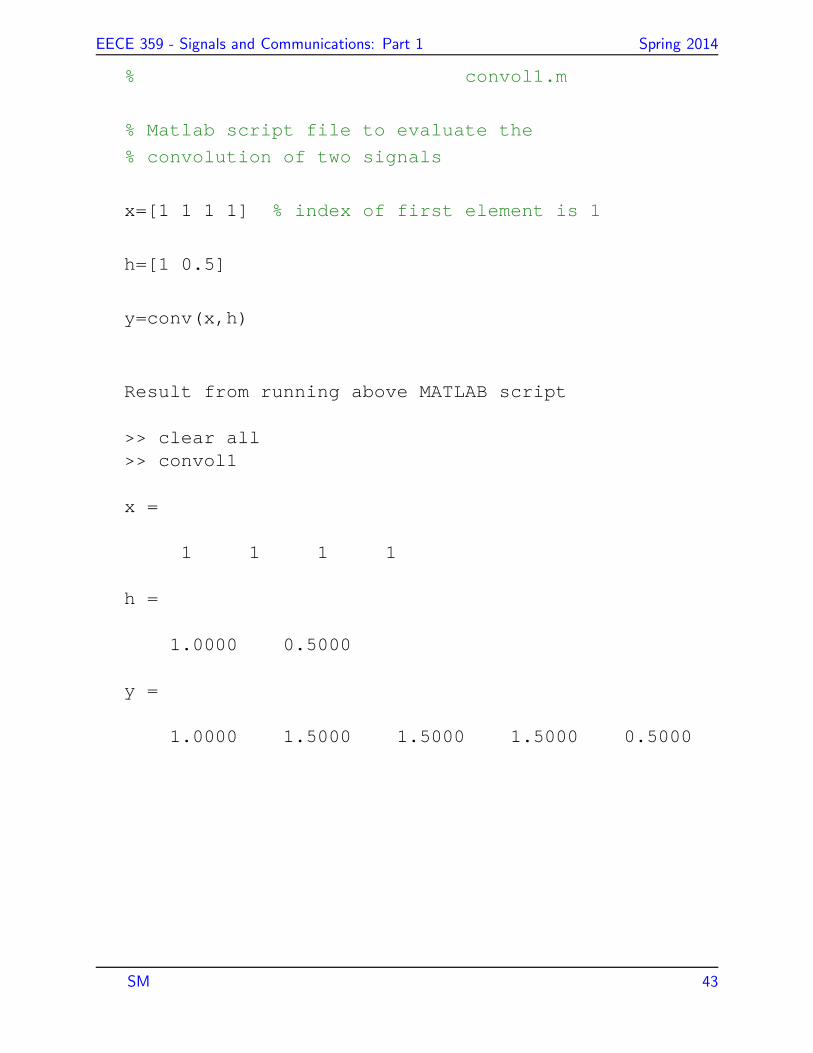
% convol1.m
% Matlab script file to evaluate the
% convolution of two signals
x=[1 1 1 1] % index of first element is 1
h=[1 0.5]
y=conv(x,h)
Result from running above MATLAB script
>> clear all>> convol1
x =
1 1 1 1
h =
1.0000 0.5000
y =
1.0000 1.5000 1.5000 1.5000 0.5000
SM 43

EECE 359 - Signals and Communications: Part 1 Spring 2014
k
1
10
1– 2
x k[ ]
32–
k
1
10
1– 2
h n k–[ ]
32–
4 5
0.5
4
for n = −1
n
1
10
1– 2
y n[ ]
32– 4 5 6
2
SM 44

EECE 359 - Signals and Communications: Part 1 Spring 2014
Continuous-time LTI systems – Section 2.2
In a manner analogous to the DT case, it
can be shown that the output y(t) of a CT
LTI system with input x(t) and unit impulse
response h(t), as depicted in the following
figure, is given by the convolution integral,
i.e.
y(t) =
∫ ∞
−∞
x(τ)h(t − τ) dτ
x t( ) y t( )LTIh t( )
We say that y(t) is the convolution of x(t) and
h(t); this relationship is commonly written as
y(t) = x(t) ∗ h(t).
SM 45
EECE 359 - Signals and Communications: Part 1 Spring 2014
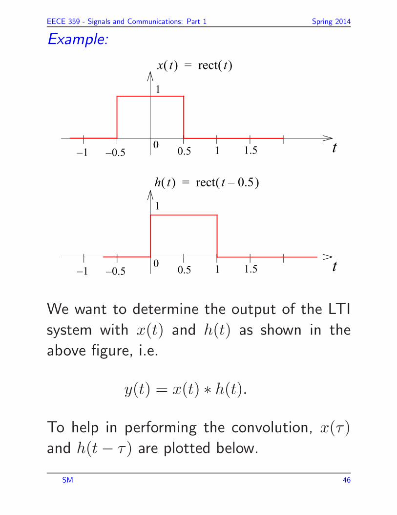
Example:
t
1
0.50
0.5– 1
x t( ) rect t( )=
1.51–
t
1
0.50
0.5– 1
h t( ) rect t 0.5–( )=
1.51–
We want to determine the output of the LTI
system with x(t) and h(t) as shown in the
above figure, i.e.
y(t) = x(t) ∗ h(t).
To help in performing the convolution, x(τ)
and h(t− τ) are plotted below.
SM 46

EECE 359 - Signals and Communications: Part 1 Spring 2014
1
0.50
0.5– 1
x τ( )
1.51–
1
0
h t τ–( )
τ
τt
t 1–
We need to evaluate
y(t) =
∫ ∞
−∞
x(τ)h(t− τ) dτ .
• Case 1: t ≤ −0.5
SM 47

EECE 359 - Signals and Communications: Part 1 Spring 2014
• Case 2: −0.5 ≤ t ≤ 0.5
• Case 3: 0.5 ≤ t ≤ 1.5
• Case 4: t ≥ 1.5
The output y(t) is sketched below.
t
1
0.50
0.5– 1
y t( )
1.51–
SM 48
EECE 359 - Signals and Communications: Part 1 Spring 2014
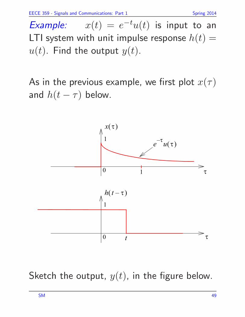
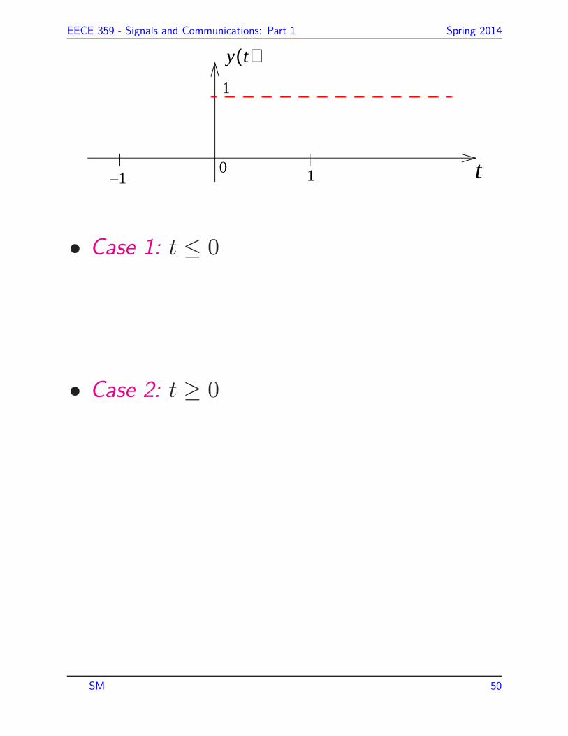
Example: x(t) = e−tu(t) is input to an
LTI system with unit impulse response h(t) =
u(t). Find the output y(t).
As in the previous example, we first plot x(τ)
and h(t− τ) below.
1
0
x τ( )
1
0
h t τ–( )
τ
τt
1
eτ–u τ( )
Sketch the output, y(t), in the figure below.
SM 49
EECE 359 - Signals and Communications: Part 1 Spring 2014
t
1
0 1
y t( )
1–
• Case 1: t ≤ 0
• Case 2: t ≥ 0
SM 50
EECE 359 - Signals and Communications: Part 1 Spring 2014
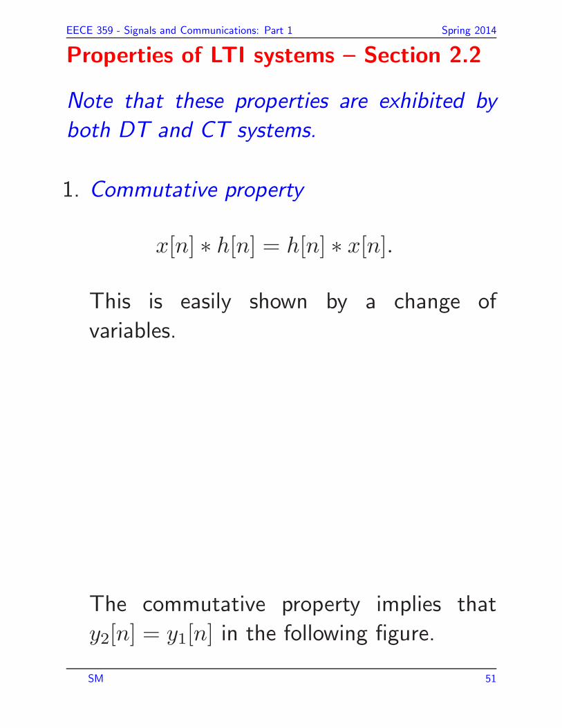
Properties of LTI systems – Section 2.2
Note that these properties are exhibited by
both DT and CT systems.
1. Commutative property
x[n] ∗ h[n] = h[n] ∗ x[n].
This is easily shown by a change of
variables.
The commutative property implies that
y2[n] = y1[n] in the following figure.
SM 51

EECE 359 - Signals and Communications: Part 1 Spring 2014
x n[ ] y1 n[ ]LTIh n[ ]
h n[ ] y2 n[ ]LTIx n[ ]
Illustrating a consequence of the commutative
property
2. Distributive property
x[n] ∗ {h1[n] + h2[n]}
= x[n] ∗ h1[n] + x[n] ∗ h2[n].
This equation states that convolution
distributes over addition.
One interpretation of this result is that the
outputs of the two systems shown in the
SM 52

EECE 359 - Signals and Communications: Part 1 Spring 2014
figure below are identical, i.e. ya[n] =
yb[n].
x n[ ]
y1 n[ ]LTIh1 n[ ]
y2 n[ ]LTIh2 n[ ]
+ya n[ ]
LTIh1 n[ ] h+
2n[ ]
x n[ ] yb n[ ]
Illustrating a consequence of the distributive property
3. Associative property
x[n] ∗ {h1[n] ∗ h2[n]}
= {x[n] ∗ h1[n]} ∗ h2[n]. (3)
Equation (3) states that the order in
SM 53
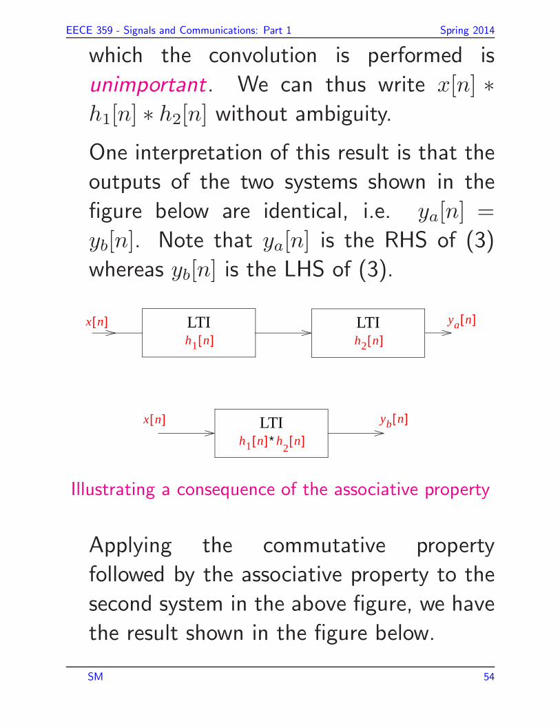
EECE 359 - Signals and Communications: Part 1 Spring 2014
which the convolution is performed is
unimportant. We can thus write x[n] ∗
h1[n] ∗ h2[n] without ambiguity.
One interpretation of this result is that the
outputs of the two systems shown in the
figure below are identical, i.e. ya[n] =
yb[n]. Note that ya[n] is the RHS of (3)
whereas yb[n] is the LHS of (3).
x n[ ] LTIh1 n[ ]
LTIh2 n[ ]
ya n[ ]
LTIh1 n[ ]∗h
2n[ ]
x n[ ] yb n[ ]
Illustrating a consequence of the associative property
Applying the commutative property
followed by the associative property to the
second system in the above figure, we have
the result shown in the figure below.
SM 54

EECE 359 - Signals and Communications: Part 1 Spring 2014
x n[ ] LTIh2 n[ ]
LTIh1 n[ ]
yd n[ ]
LTIh2 n[ ]∗h
1n[ ]
x n[ ] yc n[ ]
Re-ordering of cascade of LTI systems
We can therefore conclude that the unit
impulse response of a cascade of LTI
systems does not depend on the order in
which they are cascaded.
SM 55

EECE 359 - Signals and Communications: Part 1 Spring 2014
Unit impulse responses of various types
of LTI systems
Memoryless systems – Section 2.3.4
Necessary and sufficient conditions are:
DT : h[n] = K · δ[n]
CT : h(t) = K · δ(t).
Invertible systems – Section 2.3.5
A system is invertible if different inputs
produce different outputs. This means that
we can recover the input signal exactly from
the output signal.
Fact: An invertible LTI system has an LTI
inverse. (Problem 2.50)
Given an invertible LTI system with unit
impulse response h[n] or h(t), the unit
impulse response h1[n] or h1(t) of the inverse
SM 56

EECE 359 - Signals and Communications: Part 1 Spring 2014
system must satisfy
DT : h[n] ∗ h1[n] = δ[n]
CT : h(t) ∗ h1(t) = δ(t).
Example:
h[n] = δ[n− n0] and h1[n] = δ[n+ n0].
Causal systems – Section 2.3.6
Necessary and sufficient conditions are:
DT : h[n] = 0 for n < 0
CT : h(t) = 0 for t < 0.
Example:
h[n] = δ[n]− δ[n− 1].
SM 57

EECE 359 - Signals and Communications: Part 1 Spring 2014
Stable systems – Section 2.3.7
Necessary and sufficient conditions are:
DT :∞∑
n=−∞
|h[n]| < ∞.
The above equation states that the unit
impulse response is absolutely summable.
CT :
∫ ∞
−∞
|h(t)| dt < ∞.
The above equation states that the unit
impulse response is absolutely integrable.
Example:
h[n] = δ[n]− δ[n− 1] is stable.
h[n] = u[n] corresponds to an accumulator
and is not stable.
SM 58

EECE 359 - Signals and Communications: Part 1 Spring 2014
Summary
Property Discrete-time LTI system Continuous-time LTI system
Memoryless h[n] = δ[n] h(t) = δ(t)Invertibility h[n] ∗ hinv[n] = δ[n] h(t) ∗ hinv(t) = δ(t)Causal h[n] = 0, for n < 0 h(t) = 0, for t < 0
Stability∞∑
n=−∞|h[n]| < ∞
∞∫
−∞|h(τ)| dτ < ∞
Unit Step-Response of LTI Systems –
Section 2.3.8
It can be used as an alternative to impulse
response and uniquely describes the behaviour
of LTI systems.
Unit step response = s(t) or s[n] = system
response to input u(t) or u[n]
Relationship:
s(t) = u(t) ∗ h(t) = h(t) ∗ u(t) =
t∫
−∞
h(τ) dτ
s[n] = u[n] ∗ h[n] = h[n] ∗ u[n] =n∑
k=−∞
h[k]
SM 59

EECE 359 - Signals and Communications: Part 1 Spring 2014
andh(t) = ds(t)
t = s(t)
h[n] = s[n]− s[n− 1]
Example:
RC circuit
• Impulse response: h(t) = 1RC e−t/(RC)u(t)
• Step response: s(t) = 1RC
t∫
0
e−τ/(RC) dτ
= 1RC (−RC) e−τ/(RC)
∣∣∣∣∣
t
0
= (1− e−t/(RC))× u(t)
SM 60

EECE 359 - Signals and Communications: Part 1 Spring 2014
Systems described by differential and
difference equations – Section 2.4
Many systems and physical phenomena can
be modelled by linear constant-coefficient
difference (when the system is discrete time)
or differential (when the system is continuous
time) equations.
In general to solve difference or differential
equations we need to know the initial
conditions (e.g., initial energy of the system).
• General N th order linear constant-
coefficient differential equation
N∑
k=0
akdky(t)
dtk=
M∑
k=0
bkdkx(t)
dtk
• Solution:
y(t) = yh(t) + yp(t)
SM 61

EECE 359 - Signals and Communications: Part 1 Spring 2014
– Homogeneous solution
N∑
k=0
akdkyh(t)
dtk= 0
– Particular solution
any solution yp(t) for given x(t)
– Condition of initial rest: If x(t) = 0 for
t < t0 then
y(t)∣∣t−0
=dy(t)
dt
∣∣∣t−0
= . . . =dN−1y(t)
dtN−1
∣∣∣t−0
= 0
(corresponds to causal LTI system)
• Differential equation + initial condition
specify system output completely
SM 62
EECE 359 - Signals and Communications: Part 1 Spring 2014
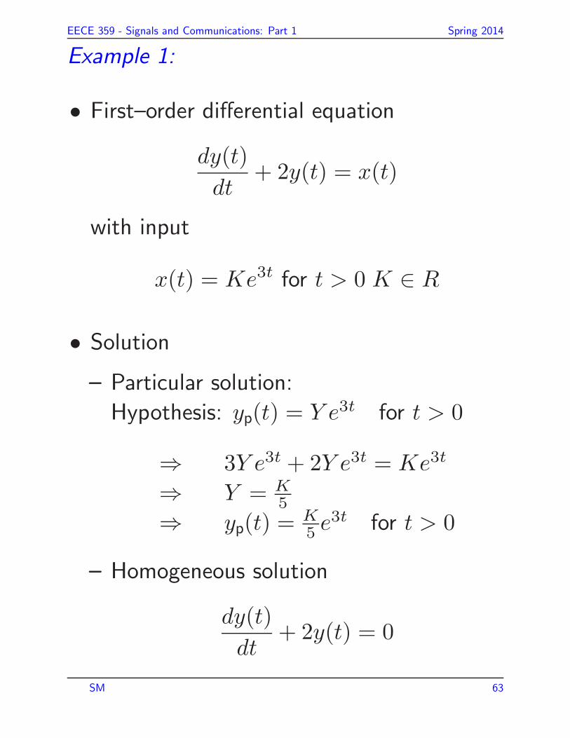
Example 1:
• First–order differential equation
dy(t)
dt+ 2y(t) = x(t)
with input
x(t) = Ke3t for t > 0 K ∈ R
• Solution
– Particular solution:
Hypothesis: yp(t) = Y e3t for t > 0
⇒ 3Y e3t + 2Y e3t = Ke3t
⇒ Y = K5
⇒ yp(t) =K5 e
3t for t > 0
– Homogeneous solution
dy(t)
dt+ 2y(t) = 0
SM 63

EECE 359 - Signals and Communications: Part 1 Spring 2014
Hypothesis: yh(t) = Aest
⇒ Asest + 2Aest = 0
⇒ s = −2
⇒ yh(t) = Ae−2t for t > 0
SM 64

EECE 359 - Signals and Communications: Part 1 Spring 2014
– Combination
y(t) = Ae−2t +K
5e3t for t > 0
– Condition of initial rest
y(t) = 0 for t < 0 since x(t) = 0 for t < 0
No impulse introduced at t = 0 ⇒
y(0) = 0
⇒ A+K
5= 0
– Complete solution
y(t) = yh(t) + yp(t)
=K
5(e3t − e−2t) for t > 0
Linear Constant-Coefficient Difference Equations
SM 65
EECE 359 - Signals and Communications: Part 1 Spring 2014
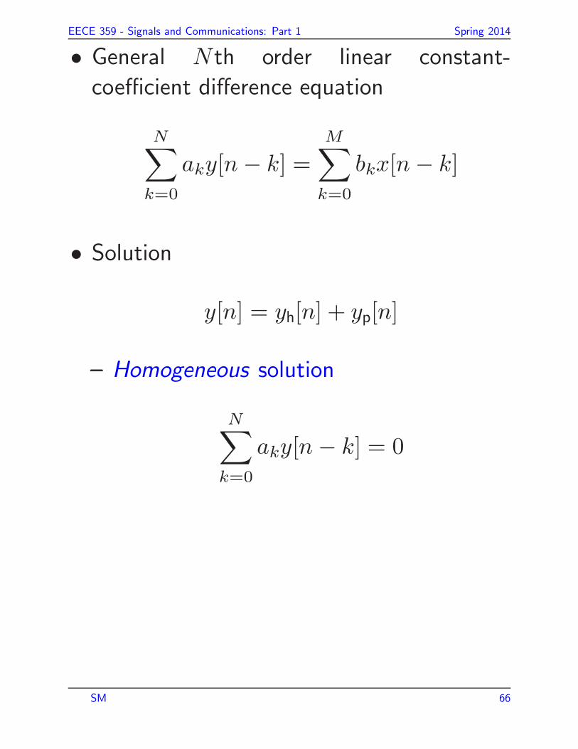
• General N th order linear constant-
coefficient difference equation
N∑
k=0
aky[n− k] =M∑
k=0
bkx[n− k]
• Solution
y[n] = yh[n] + yp[n]
– Homogeneous solution
N∑
k=0
aky[n− k] = 0
SM 66

EECE 359 - Signals and Communications: Part 1 Spring 2014
– Particular solution
any solution yp[n] for given x[n]
– Condition of initial rest: If x[n] = 0 for
n < n0 then
y[n] = 0 for n < n0
(corresponds to causal LTI system)
• Alternatively: rewrite difference equation
y[n] =1
a0
(M∑
k=0
bkx[n− k]−N∑
k=1
aky[n− k]
)
and solve for successive values of n ≥ n0
Example 2:
1. Assume nonrecursive difference equation
y[n] = x[n]− x[n− 1]
SM 67

EECE 359 - Signals and Communications: Part 1 Spring 2014
Impulse response of underlying LTI system
obtained for
x[n] = δ[n]
⇒ y[n] = h[n] = δ[n]− δ[n− 1]
Since h[n] = 0 for n > 2 the underlying
system is referred to as finite impulse
response (FIR) system.
2. Consider recursive difference equation
y[n]−1
2y[n− 1] = x[n]
or
y[n] = x[n] +1
2y[n− 1]
Impulse response of underlying LTI system
(Condition of initial rest: y[n] = 0 for
SM 68

EECE 359 - Signals and Communications: Part 1 Spring 2014
n < 0)
y[0] = x[0] +1
2y[−1] = 1
y[1] = x[1] +1
2y[0] =
1
2
y[2] = x[2] +1
2y[1] =
1
4· · ·
y[n] = x[n] +1
2y[n− 1] =
(1
2
)n
⇒ impulse response h[n] = (1/2)nu[n]
Since h[n] has an infinite duration, the
underlying system is referred to as infinite
impulse response (IIR) system.
SM 69

EECE 359 - Signals and Communications: Part 1 Spring 2014
Fourier series representation of periodic
signals – Chapter 3
We have seen that a signal can generally be
represented as a linear combination of shifted
impulse (or sample) functions.
We will show that a signal can also
be represented as a linear combination
of complex exponential functions, provided
certain conditions are satisfied.
Why is this useful? Section 3.2
Reason is due to this important fact: The
output of an LTI system due to a complex
exponential input is the same complex
exponential multiplied by a (possibly complex)
gain factor.
We say that complex exponentials are
eigenfunctions of LTI systems; the gain
factors are termed eigenvalues. (cf.
SM 70

EECE 359 - Signals and Communications: Part 1 Spring 2014
eigenvectors and eigenvalues of a matrix)
We now prove the following.
Continuous-time: If x(t) = est is input to a
LTI system with impulse response h(t), the
output y(t) is
y(t) = H(s)est
where
H(s) =
∫ ∞
−∞
h(τ) e−sτ dτ
Proof:
SM 71

EECE 359 - Signals and Communications: Part 1 Spring 2014
Example:
Suppose y(t) = x(t− 1) and x(t) = ej2πt.
Example:
Suppose y(t) = x(t−1) and x(t) = cos 2πt+
cos 3πt.
SM 72

EECE 359 - Signals and Communications: Part 1 Spring 2014
Discrete-time: If x[n] = zn is input to a
LTI system with impulse response h[n], the
output y[n] is
y[n] = H(z)zn
where
H(z) =∞∑
k=−∞
h[k] z−k
Proof:
SM 73

EECE 359 - Signals and Communications: Part 1 Spring 2014
Fourier series representation of CT
periodic signals – Section 3.3
Let x(t) be a periodic signal with fundamental
period T . Then if certain conditions
(Dirichlet, pp. 197-200) are satisfied, we can
represent x(t) as a Fourier series (FS) (an
infinite sum of complex exponentials):
x(t) =
∞∑
k=−∞
ak ejk(2πT )t
where the (possibly complex) Fourier
coefficients {ak} are given by
ak =1
T
∫ T2
−T2
x(t) e−jk(2πT )t dt,
k = 0,±1,±2, . . .
The above equations are referred to as the
synthesis and analysis equations respectively.
SM 74

EECE 359 - Signals and Communications: Part 1 Spring 2014
Section 3.4 provides a good discussion of the
convergence of the FS representation.
Notes:
1. Using Euler’s relationship, we can also
express the FS representation as an infinite
sum of sine and cosine terms.
2. Given x(t), we can determine {ak}∞k=−∞;
conversely, we can reconstruct x(t) from
{ak}∞k=−∞.
{ak}∞k=−∞ give the frequency-domain
description of the signal and are called its
spectral coefficients.
3. A periodic signal x(t) of fundamental
period T has components at frequencies
0,±2πT ,±4π
T , . . ., i.e. at multiples of the
fundamental frequency ω0 =2πT or f0 =
1T .
SM 75

EECE 359 - Signals and Communications: Part 1 Spring 2014
The component at freq nf0 is called the
nth harmonic .
4. Conjugate symmetry property: If x(t) is
real, then a−k = a∗k.
Proof:
As a result,
|a−k| = |a∗k| = |ak|
and ∠a−k = ∠a∗k = −∠ak .
SM 76
EECE 359 - Signals and Communications: Part 1 Spring 2014
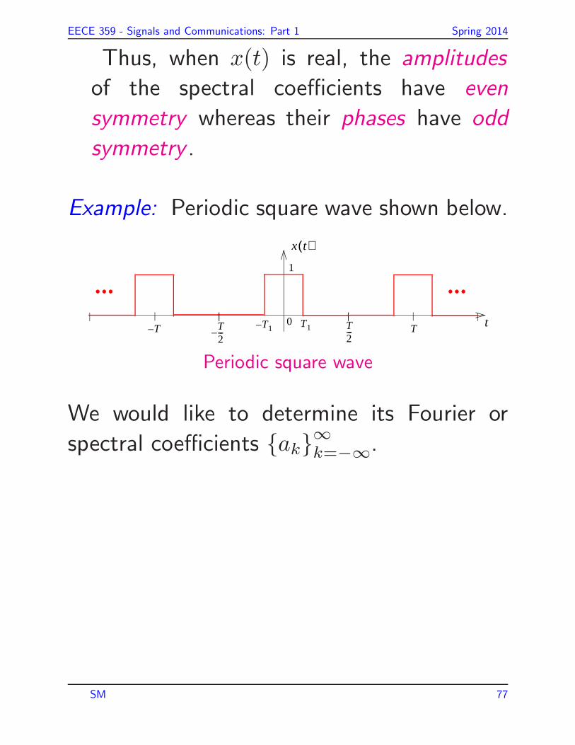
Thus, when x(t) is real, the amplitudes
of the spectral coefficients have even
symmetry whereas their phases have odd
symmetry .
Example: Periodic square wave shown below.
1
T10T1– T
2---
x t( )
T2---–
tTT–
Periodic square wave
We would like to determine its Fourier or
spectral coefficients {ak}∞k=−∞.
SM 77