NOTES ON HEAT KERNEL ASYMPTOTICS

DANIEL GRIESER

Abstract. These are informal notes on how one can prove the existence and

asymptotics of the heat kernel on a compact Riemannian manifold with bound-

ary. The method differs from many treatments in that neither pseudodiffer-ential operators nor normal coordinates are used; rather, the heat kernel is

constructed directly, using only a first (Euclidean) approximation and a Neu-mann (Volterra) series that removes the errors.

Contents

1. Introduction 22. Manifolds without boundary 52.1. Outline of the proof 52.2. The heat calculus 62.3. The Volterra series 102.4. Proof of the Theorem of Minakshisundaram-Pleijel 122.5. More remarks: Formulas, generalizations etc. 123. Manifolds with boundary 163.1. The boundary heat calculus 173.2. The Volterra series 243.3. Construction of the heat kernel 24References 26

Date: August 13, 2004.

1

2 DANIEL GRIESER

1. Introduction

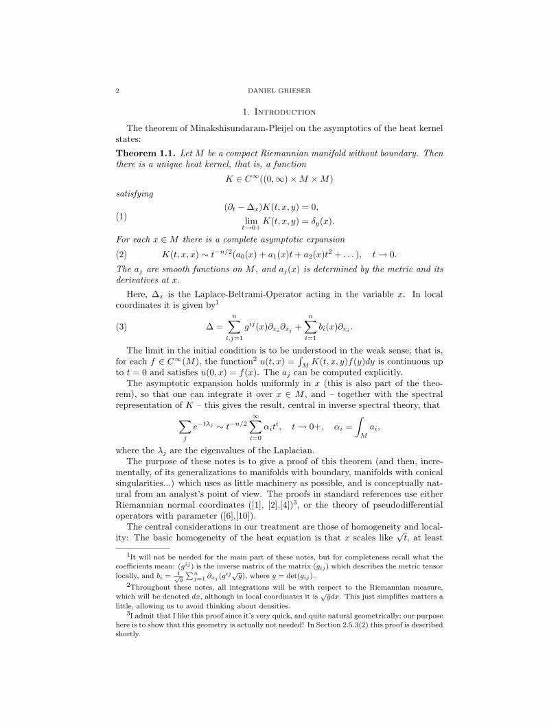
The theorem of Minakshisundaram-Pleijel on the asymptotics of the heat kernelstates:

Theorem 1.1. Let M be a compact Riemannian manifold without boundary. Thenthere is a unique heat kernel, that is, a function

K ∈ C∞((0,∞)×M ×M)

satisfying(∂t −∆x)K(t, x, y) = 0,

limt→0+

K(t, x, y) = δy(x).(1)

For each x ∈M there is a complete asymptotic expansion

(2) K(t, x, x) ∼ t−n/2(a0(x) + a1(x)t+ a2(x)t2 + . . . ), t→ 0.

The aj are smooth functions on M , and aj(x) is determined by the metric and itsderivatives at x.

Here, ∆x is the Laplace-Beltrami-Operator acting in the variable x. In localcoordinates it is given by1

(3) ∆ =n∑

i,j=1

gij(x)∂xi∂xj

+n∑

i=1

bi(x)∂xi.

The limit in the initial condition is to be understood in the weak sense; that is,for each f ∈ C∞(M), the function2 u(t, x) =

∫MK(t, x, y)f(y)dy is continuous up

to t = 0 and satisfies u(0, x) = f(x). The aj can be computed explicitly.The asymptotic expansion holds uniformly in x (this is also part of the theo-

rem), so that one can integrate it over x ∈ M , and – together with the spectralrepresentation of K – this gives the result, central in inverse spectral theory, that∑

j

e−tλj ∼ t−n/2∞∑

i=0

αiti, t→ 0+, αi =

∫M

ai,

where the λj are the eigenvalues of the Laplacian.The purpose of these notes is to give a proof of this theorem (and then, incre-

mentally, of its generalizations to manifolds with boundary, manifolds with conicalsingularities...) which uses as little machinery as possible, and is conceptually nat-ural from an analyst’s point of view. The proofs in standard references use eitherRiemannian normal coordinates ([1], [2],[4])3, or the theory of pseudodifferentialoperators with parameter ([6],[10]).

The central considerations in our treatment are those of homogeneity and local-ity: The basic homogeneity of the heat equation is that x scales like

√t, at least

1It will not be needed for the main part of these notes, but for completeness recall what the

coefficients mean: (gij) is the inverse matrix of the matrix (gij) which describes the metric tensor

locally, and bi = 1√g

∑nj=1 ∂xj (gij√g), where g = det(gij).

2Throughout these notes, all integrations will be with respect to the Riemannian measure,

which will be denoted dx, although in local coordinates it is√gdx. This just simplifies matters a

little, allowing us to avoid thinking about densities.3I admit that I like this proof since it’s very quick, and quite natural geometrically; our purpose

here is to show that this geometry is actually not needed! In Section 2.5.3(2) this proof is describedshortly.

NOTES ON HEAT KERNEL ASYMPTOTICS 3

in the leading terms (i.e. forgetting the terms imvolving bi in (3)). This, alongwith the initial condition, leads one to expect that K(t, x, y) should be expressible’nicely’ in terms of the new variable X = (x − y)/

√t, in local coordinates. This

expectation is supported by the well-known formula

(4) E(t, x, y) =1

(4πt)n/2e−|x−y|2/4t

for the heat kernel on Rn, with the Euclidean metric.4 Locality is the rapid decayof E as function of (x− y)/

√t.

We will define spaces of functions, ΨαH(M), α ∈ −N0/2, which reflect this ho-

mogeneity and locality of E. The ’order’ α encodes the leading power of t, and isnormalized so that E ∈ Ψ−1

H (Rn). The existence part of Theorem 1.1 will followfrom the construction of a heat kernel K ∈ Ψ−1

H (M). The letter Ψ is supposed toshow the close analogy of our approach to the parametrix construction for ellipticoperators in the pseudodifferential calculus. In fact, the procedure is exactly thesame, except that here in the heat equation context the details are much easier!5.

The reader is not assumed to be familiar with the pseudodifferential calculus.Neither will she learn it here. But still she will learn some of the main ideas involvedin it, without having to bother with technicalities like distributions or oscillatoryintegrals.

The approach followed here was inspired by the treatment of R. Melrose in [13],Sections 7.1-7.3. We deviate from his treatment by proving a composition formulaand using the Volterra series directly, instead of using a recursive procedure (whichwe also describe shortly in Section 2.5). Our purpose is to explain this methodin simple terms, avoiding the somewhat arcane language used in Melrose’s book.6

However, the interested reader should definitely consult that book!7

The boundary value problem is then treated in a similar manner. It is remark-able that, after initial basic homogeneity and locality considerations, only minormodifications are needed to treat this more general case. The treatment of theboundary value problem by this method seems to be new. (The ’b’ in ’b-calculus’,as treated in [13], Sections 7.4-7.5, also refers to a manifold with boundary, butto a different class of metrics (infinite cylindrical ends), which yields a differentanalysis.)

Generalizations: The method presented here works with any elliptic (in asuitable sense) operator replacing the Laplacian. That is, one can treat higherorder operators and systems (i.e. operators acting between vector bundles) in the

4Actually, the heat kernel on Rn is only unique if one imposes certain growth conditions for

x − y → ∞. The homogeneity holds precisely in Rn, and means that if K(t, x, y) satisfies (1)

then so does λnK(λ2t, λx, λy) for any λ > 0 (recall that δ(λx) = λ−nδ(x)). Set λ = t−1/2 and

use uniqueness to see that K equals t−n/2 times a function of x/√t, y/

√t. Similarly, translation

invariance shows that the latter is actually a function of (x− y)/√t, and rotation invariance that

it is a radial function; putting this into (1) one obtains an ordinary differential equation for this

function, which can be solved easily.5In particular, this approach is more direct and simpler than the more standard approach

in which first a parametrix for the resolvent is constructed as pseudodifferential operator with

parameter, and then an inverse Laplace transform is applied to obtain the heat kernel.6But keep in mind that we are doing this in hopes that a similar treatment is possible for

’singular manifolds’, and for these it may well be advantageous to use this language!7Essentially the same method of proof is used by McKean and Singer [12] (with many details

missing).

4 DANIEL GRIESER

same way. In particular, self-adjointness is not needed. See Section 2.5. (This istrue at least for the part without boundary, and, with more modifications, alsofor boundary problems). See also [7], which has a quick treatment (in the casewithout boundary) using pseudodifferential operators (and a not so quick one withboundary).

Also, one can deal with limited smoothness, since the Volterra series only in-volves integrations. To determine the minimal smoothness required in the proofof existence, and to have a given number of terms in the expansion, is left as anexercise.

NOTES ON HEAT KERNEL ASYMPTOTICS 5

2. Manifolds without boundary

In this section we give a detailed analysis of the heat kernel on a compact Rie-mannian manifold without boundary. This will imply the theorem of Minakshisundaram-Pleijel.

2.1. Outline of the proof. Our basic strategy in the proof of Theorem 1.1 followsthe following standard pattern:

(1) Construct an approximate heat kernel (parametrix) K1, in the sense that

(∂t −∆x)K1(t, x, y) = R(t, x, y)

limt→0+

K1 = δy(x)(5)

with R ’small’ in a sense to be specified later.(2) Correct K1 to an exact heat kernel, by summing a convergent series (the

Volterra series). This proves existence of a heat kernel, satisfying theasymptotics (2).

(3) Uniqueness can be derived from existence via duality (using self-adjointness),or proved via an energy estimate.

The obvious candidate for a first approximation is given by the Euclidean heatkernel (4). More precisely, if one wants the approximation to be good near x = y(and near t = 0), for each y, then one should use the metric g(y) here8. That is, if

(6) E(g)(t, x, y) =1

(4πt)n/2e−|x−y|2g/4t,

|x|g :=∑n

i,j=1 gijxixj , denotes the heat kernel for the ’constant’ metric g = (gij),gij ∈ R, on Rn, then one may hope that

(7) K1(t, x, y) = E(g(y))(t, x, y)

(in local coordinates onM , and then suitably patched together) is an approximationto the true heat kernel. Indeed, an easy calculation (see Proposition 2.7) showsthat (∂t−∆x)K1 equals t−n/2−1/2 times a smooth function of t, (x−y)/

√t, y. This

is ’good’ since ∂tK1 and ∆xK1 separately would have the more singular factor9

t−n/2−1.The simple argument for the second step, how to ’iterate away the error terms’,

will be recalled in Section 2.3. This works most easily, and is standard, if R in (5)remains bounded as t→ 0. But we just saw that R can definitely not be expectedto be bounded if K1 is taken as in (7)! So we need

(1) either a better parametrix in the first step,

8It is in this refinement in the very first step that, in the analogous construction of a parametrixfor an elliptic operator, the pseudodifferential technique differs from (and improves upon) the

classical method of (i) freezing coefficients at points in an ε-net on M , (ii) inverting the resulting

constant coefficient operators in Rn and transferring the solutions to ε-neighborhoods of thesepoints, and (iii) patching these local approximate solutions together. This method yields an error

term of type ’small norm (for small ε) operator plus lower order operator’. In contrast, the ΨDO

parametrix yields only a lower order, hence compact, error. While the classical method sufficesto prove discreteness of the spectrum, for example, the ΨDO method is superior if one wants to

obtain more refined quantitative information, for example the Weyl asymptotics with error term.9We will see that, for this to be true, K1 essentially (i.e. up to lower order terms) has to be

chosen as in (7). So there is no guessing involved here, really!

6 DANIEL GRIESER

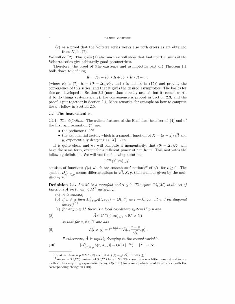
(2) or a proof that the Volterra series works also with errors as are obtainedfrom K1 in (7).

We will do (2). This gives (1) also since we will show that finite partial sums of theVolterra series give arbitrarily good parametrices.

Therefore, the proof of (the existence and asymptotics part of) Theorem 1.1boils down to defining

K = K1 −K1 ∗R+K1 ∗R ∗R− . . .

(where K1 is (7), R = (∂t − ∆x)K1, and ∗ is defined in (15)) and proving theconvergence of this series, and that it gives the desired asymptotics. The basics forthis are developed in Section 2.2 (more than is really needed, but it seemed worthit to do things systematically), the convergence is proved in Section 2.3, and theproof is put together in Section 2.4. More remarks, for example on how to computethe ai, follow in Section 2.5.

2.2. The heat calculus.

2.2.1. The definition. The salient features of the Euclidean heat kernel (4) and ofthe first approximation (7) are:

• the prefactor t−n/2

• the exponential factor, which is a smooth function of X = (x− y)/√t and

y, exponentially decaying as |X| → ∞.It is quite clear, and we will compute it momentarily, that (∂t − ∆x)K1 will

have the same form, except for a different power of t in front. This motivates thefollowing definition. We will use the following notation:

C∞([0,∞)1/2)

consists of functions f(t) which are smooth as functions10 of√t, for t ≥ 0. The

symbol Dγ√t,X,y

means differentiations in√t,X, y, their number given by the mul-

tiindex γ.

Definition 2.1. Let M be a manifold and α ≤ 0. The space ΨαH(M) is the set of

functions A on (0,∞)×M2 satisfying:(a) A is smooth,(b) if x 6= y then Dγ

t,x,yA(t, x, y) = O(t∞) as t → 0, for all γ, (’off diagonaldecay’) 11

(c) for any p ∈M there is a local coordinate system U 3 p and

(8) A ∈ C∞([0,∞)1/2 × Rn × U)

so that for x, y ∈ U one has

(9) A(t, x, y) = t−n+2

2 −αA(t,x− y√

t, y).

Furthermore, A is rapidly decaying in the second variable:

(10) |Dγ√t,X,y

A(t,X, y)| = O(|X|−∞), |X| → ∞,

10that is, there is g ∈ C∞(R) such that f(t) = g(√t) for all t ≥ 0.

11We write ’O(t∞)’ instead of ’O(tN ) for all N ’. This condition is a little more natural in our

method than requiring exponential decay, O(e−c/t) for some c, which would also work (with the

corresponding change in (10)).

NOTES ON HEAT KERNEL ASYMPTOTICS 7

for all γ, uniformly for bounded t and y.

Note that (c) implies (b) for x, y ∈ U .Clearly, Ψα

H ⊃ Ψα−1/2H .

Remark: The funny normalization of the order α (leading to the unpleasantexponent of t in (9)) is motivated by the fact, proved below, that only with thisnormalization will the orders add under convolution (defined below) of such func-tions. Very negative α correspond to ’very smooth’ (at t = 0) kernels; this is chosento parallel the usual notion of order in the pseudodifferential calculus.

It will be useful to have:

Definition 2.2. Let A ∈ ΨαH(M). Given coordinates as in Definition 2.1(c), the

leading term of A, denoted12 Φα(A), is the function

(X, y) 7→ A(0, X, y),

with A given in (9).

Note that A is not defined uniquely by A: If t > 0 then (x− y)/√t assumes only

a bounded set of values! But whenever X√t is sufficiently small then

(11) A(t,X, y) = t(n+2)/2+αA(t, y +X√t, y),

so at least Φα(A) is uniquely defined.The definition of leading term depends on the choice of local coordinates (since

A does). We now analyze how.

2.2.2. Coordinate invariance.

Lemma 2.3. (a) If condition (c) in Definition 2.1 holds in one coordinatesystem then it holds in any.

(b) The leading term Φα(A) is defined invariantly as a function on the tangentbundle, rapidly decaying in the fiber direction:

(12) Φα(A) ∈ C∞S(fibers)(TM).

Proof. (a) Suppose ψ(x) = x is a coordinate change, and condition (c) holds in thex-coordinate patch U , with a function ¯A(t, X, y) satisfying (8), (10). We need tofind a function A with the same properties, and satisfying

(13) A(t,x− y√

t, y) = ¯A(t,

ψ(x)− ψ(y)√t

, ψ(y))

for all x, y near p. This is easy: Choose a smooth, matrix-valued function h satis-fying

ψ(x)− ψ(y) = h(x, y)(x− y)and13 h(y, y) = dψ|y, and a cutoff function χ ∈ C∞0 (U), equal to one near p, andthen set

(14) A(t,X, y) = ¯A(t, h(y +X√t, y)X,ψ(y))χ(y +X

√t),

which is clearly equivalent to (13), for y, y +X√t near p.

12The letter Φ is supposed to reflect the German ’Fuhrender Term’. Melrose calls this the

normal operator.13h(x, y) =

∫ 10 dψ|y+t(x−y)dt will do

8 DANIEL GRIESER

(b) From (14) and h(y, y) = dψy we have A(0, X, y) = ¯A(0, dψy(X), ψ(y)), whichwas to be shown.14

Note that even if ¯A was smooth in t (rather than√t) then A would still be

only smooth in√t. So for a coordinate invariant definition we need to allow

√t-

dependence. Below we will see why in the final result, Theorem 1.1, only integralpowers appear.

The higher order derivatives ∂m√tA(0, X, y) are also determined by A, but depend

on the choice of coordinates in a more complicated way. We won’t need these here.

2.2.3. Short exact sequence. The following lemma is quite obvious, but central toany type of ’step by step improvement’ argument:

Lemma 2.4. (a) Let A ∈ ΨαH . Then Φα(A) = 0 iff A ∈ Ψα−1/2

H .(b) Given a function F ∈ C∞S(fibers)(TM), and α ∈ R, there is A ∈ Ψα

H(M)having F as leading term.

In other words, one has an exact sequence, for each α,

0 → Ψα−1/2H (M) → Ψα

H(M) Φα→ C∞S(fibers)(TM) → 0.

2.2.4. Composition. We now prove that ΨαH behaves well under composition of

operators. As we will see in Section 2.3, the appropriate notion of composition hereis:

Definition 2.5. The convolution product of two smooth functions A, B on (0,∞)×M2 is the function, on the same space,

(15) (A ∗B)(t, x, y) =∫ t

0

∫M

A(t− s, x, z)B(s, z, y) dzds,

whenever the integrals are absolutely convergent.

If one considers functions A(t, x, y) as Schwartz kernels of time-dependent fami-lies of operators via (A(t)f)(x) =

∫MA(t, x, y)f(y) dy, and if one sets A(t) = 0 for

t < 0 then this is just the usual convolution of functions on R valued in a ring (thering of operators). Equivalently, if one associates with A(t, x, y) the operator onR×M whose Schwartz kernel is (s, t, x, y) 7→ A(t− s, x, y)H(t− s) (where H is thecharacteristic function of the positive half line) then ∗ is just composition on thelevel of such Schwartz kernels.

Proposition 2.6. Let A ∈ ΨαH(M), B ∈ Ψβ

H(M), with α, β < 0, and assumeM is compact. Then A ∗ B is defined and lies in Ψα+β

H (M). The leading termsa = Φα(A), b = Φβ(B), a ∗ b := Φα+β(A ∗B) satisfy(16)

(a ∗ b)(X, y) =∫ 1

0

∫Rn

(1− σ)−(n+2)/2−ασ−(n+2)/2−βa(X − Z√

1− σ, y)b(

Z√σ, y) dZdσ.

14One could have defined the leading term without reference to coordinates, as follows: LetX ∈ TyM be the equivalence class of a curve γ, that is γ(0) = y, γ′(0) = X. Then Φα(A)(X, y) =

limt→0 t(n+2)/2+αA(t, γ(√t), y).

NOTES ON HEAT KERNEL ASYMPTOTICS 9

Proof. First, consider x, y in a coordinate patch U , where A,B have representationsas in (9) (note that we use invariance here!), and consider the part of the convolutionproduct with z near y, that is

(17)∫ t

0

∫Rn

A(t− s, x, z)B(s, z, y)χ(z) dzds

where χ ∈ C∞0 (U) is equal to one near y. We replace the integration variables byσ = s/t, Z = (z − y)/

√t and introduce the new variable X = (x − y)/

√t instead

of x. Then (17) becomes t−(n+2)/2−α−βC(t,X, y) where C(t,X, y) equals

(18)∫ 1

0

∫Rn

(1− σ)−(n+2)/2−ασ−(n+2)/2−β ·

A(t(1− σ),X − Z√

1− σ, y + Z

√t)B(tσ,

Z√σ, y)χ(y + Z

√t) dZ dσ.

Convergence and rapid decay as |X| → ∞ follow for the part σ ≤ 1/2 by introducingthe variable W = Z/

√σ for Z, then the power of σ is −1 − β, so the integral

converges since β < 0, and rapid decay as |X| → ∞ can be easily seen from|X−W

√σ√

1−σ| ≥ ||X| − |W || and rapid decay of A, B. The part σ ≥ 1/2 is treated

similarly. If χ is replaced by 1− χ then the result is rapidly decaying as t→ 0, ascan easily be seen from the rapid decay of B(1− χ) as s→ 0.

Formula (16) follows immediately from (18).Similar arguments also show smoothness and rapid decay of A ∗B for x 6= y.

The following is the central calculation for the whole heat kernel construction,and the reader should try to do it herself before (or instead of) reading the proof.

Proposition 2.7. (1) Let A ∈ ΨαH(M), α ≤ −1. Then (∂t−∆x)A ∈ Ψα+1

H (M).(2) If a = Φα(A) and r = Φα+1((∂t −∆x)A) then

(19) r(X, y) =[−n+ 2

2− α− 1

2X∂X −∆0,y

X

]a(X, y).

Here, X∂X :=∑

iXi∂Xi, and ∆0,y

X =∑

ij gij(y)∂Xi

∂Xjis the leading part of

the Laplacian, with coefficients frozen at y, acting in X.

We will only use a consequence of (19): When computing the leading term of(∂t − ∆x)A at y one may forget the lower order part of the Laplacian, the x-dependence in its leading term, and the t-dependence of A.

Proof. Write A(t, x, y) = t−lA(t, x−y√t, y), l = n+2

2 + α. We have

∂tA = −l t−l−1A− t−l x− y

2t3/2∂XF + t−l∂tA

= t−l−1(−l − 12X∂X)F +R1,

and R1 is in Ψα+1/2H (M) since ∂t = 1

2√

t∂√t.

10 DANIEL GRIESER

Next, ∂xi(t−lA) = t−l−1/2∂Xi

A, and this gives

∆xA = t−l−1∑i,j

gij(x)∂Xi∂Xj

A+ t−l−1/2∑

i

bi(x)∂XiA

= t−l−1∑i,j

gij(y)∂X1∂X2A+R2.

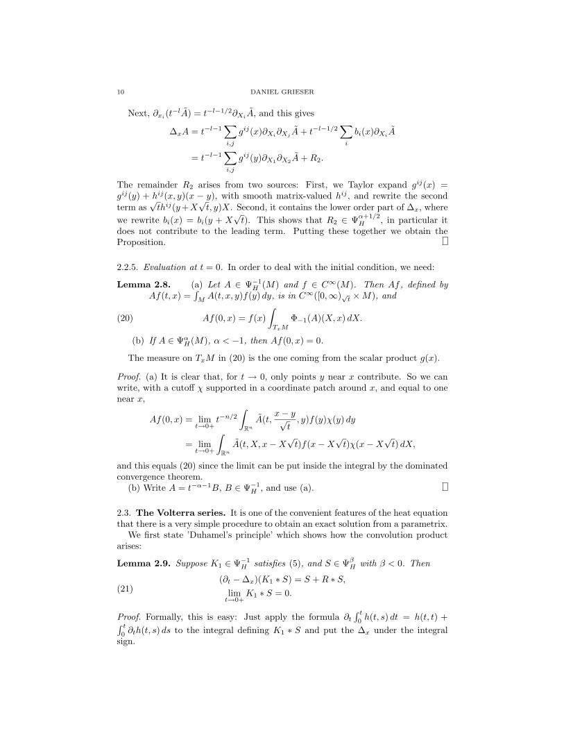
The remainder R2 arises from two sources: First, we Taylor expand gij(x) =gij(y) + hij(x, y)(x − y), with smooth matrix-valued hij , and rewrite the secondterm as

√thij(y+X

√t, y)X. Second, it contains the lower order part of ∆x, where

we rewrite bi(x) = bi(y + X√t). This shows that R2 ∈ Ψα+1/2

H , in particular itdoes not contribute to the leading term. Putting these together we obtain theProposition.

2.2.5. Evaluation at t = 0. In order to deal with the initial condition, we need:

Lemma 2.8. (a) Let A ∈ Ψ−1H (M) and f ∈ C∞(M). Then Af , defined by

Af(t, x) =∫

MA(t, x, y)f(y) dy, is in C∞([0,∞)√t ×M), and

(20) Af(0, x) = f(x)∫

TxM

Φ−1(A)(X,x) dX.

(b) If A ∈ ΨαH(M), α < −1, then Af(0, x) = 0.

The measure on TxM in (20) is the one coming from the scalar product g(x).

Proof. (a) It is clear that, for t → 0, only points y near x contribute. So we canwrite, with a cutoff χ supported in a coordinate patch around x, and equal to onenear x,

Af(0, x) = limt→0+

t−n/2

∫Rn

A(t,x− y√

t, y)f(y)χ(y) dy

= limt→0+

∫Rn

A(t,X, x−X√t)f(x−X

√t)χ(x−X

√t) dX,

and this equals (20) since the limit can be put inside the integral by the dominatedconvergence theorem.

(b) Write A = t−α−1B, B ∈ Ψ−1H , and use (a).

2.3. The Volterra series. It is one of the convenient features of the heat equationthat there is a very simple procedure to obtain an exact solution from a parametrix.

We first state ’Duhamel’s principle’ which shows how the convolution productarises:

Lemma 2.9. Suppose K1 ∈ Ψ−1H satisfies (5), and S ∈ Ψβ

H with β < 0. Then

(∂t −∆x)(K1 ∗ S) = S +R ∗ S,lim

t→0+K1 ∗ S = 0.(21)

Proof. Formally, this is easy: Just apply the formula ∂t

∫ t

0h(t, s) dt = h(t, t) +∫ t

0∂th(t, s) ds to the integral defining K1 ∗ S and put the ∆x under the integral

sign.

NOTES ON HEAT KERNEL ASYMPTOTICS 11

Really, one should be a little careful about convergence, interchanging differen-tiation and integration and such things. This is left as an exercise. 15 The initialcondition follows from Lemma 2.8(b).

In particular, for R = 0 this says: From a solution of the initial value problem (1),with the homogeneous equation, one may obtain a solution of the inhomogeneousequation, with zero initial condition, using the convolution product. The advantageof translating to the latter problem here is that an operator of the form (Identityplus small) may be inverted explicitly using the ’geometric series’, which in thiscontext is sometimes called the Volterra series.16

Denote R∗N = R ∗R ∗ · · · ∗R, with N factors.

Proposition 2.10. Assume K1 ∈ Ψ−1H satisfies (5) with R ∈ Ψ−1/2

H .(a) Then

(22) K := K1 −K1 ∗R+K1 ∗R ∗R− . . .

converges in C∞((0,∞)×M2), and K ∈ Ψ−1H (M).

(b) K is a heat kernel, that is, it satisfies (1).(c) The series (22) is an asymptotic series as t→ 0. More precisely, K1∗R∗N ∈

Ψ−1−N/2H (M).

Proof. (c) is obvious from the composition theorem, Proposition 2.6, and (b) is clearonce convergence is proven, since Duhamel’s principle gives (∂t−∆x)(K1 ∗R∗m) =R∗m +R∗(m+1), so the sum telescopes. Also, the initial condition is not affected bythe terms involving R, by Lemma 2.8(b).

Let us show uniform convergence first: Let S = R∗N , for a fixed N ≥ n/2 + 1.Then S ∈ Ψ−n/2−1

H , so S is bounded for bounded t. This gives

(23) S∗m(t, x, y) =∫

0≤t1≤···≤tm−1≤t

∫Mm−1

S(t− t1, x, z1)S(t1 − t2, z1, z2) . . .

. . . S(tm−2 − tm−1, zm−2, zm−1)S(tm−1, zm−1, y) dz1 . . . dzm−1 dt1 . . . dtm−1.

The integrand is bounded by Cm, if C is an upper bound for |S| on (0, t) ×M2,the volume of the domain of integration in the zi-variables is (volM)m−1, and thevolume in the ti-variables is tm−1/(m− 1)!, so we get

|S∗m(t, x, y)| ≤ tm−1(volM)m−1Cm

(m− 1)!.

Clearly, then, |K1 ∗ Ri+mN | has the same bound for i = N, . . . , 2N − 1 andm = 1, 2, 3, . . . , and this proves convergence in C0. Similar estimates hold withl derivatives, for any fixed l, if N is chosen as n/2 + 1 + l instead. This provesconvergence in C∞. To show K ∈ Ψ−1

H , note that we have, from the estimates

15Note that part of the statement is that R ∗ S makes sense. This does not follow from

Proposition 2.6 since R ∈ Ψ0H only! (We are not assuming anything about the form of K1,

although this generality is not needed here.) A more careful analysis shows that R ∗ S is defined

for R ∈ Ψ0H if

∫Rn R(0, X, y) dX = 0 for each y, and that this is satisfied for R arising as derivative.

16In [12], this is called Levi’s sum. A Volterra series is very similar to a Neumann series;

both invert an operator I − R as I + R + R2 + . . . . But for the Neumann series one ascertains

convergence by assuming the norm of R to be less than one (in a suitably chosen space). For theVolterra series no norm estimate is needed, the convergence follows rather from a sort of ’negative

order’ and ’Volterra’ (i.e., the integral kernel vanishes above the diagonal) condition on R.

12 DANIEL GRIESER

just proven, that for any l and N there is KN ∈ Ψ−1H with K = KN + O(tN )

in Cl. Clearly, this gives (a) and (b) in Definition 2.1. If one sets K(t,X, y) =tn/2K(t, y + X

√t, y)χ(y + X

√t) = KN (t,X, y) + O(tN+n/2)χ(y + X

√t), with a

cutoff function χ supported near y, then X ≤ Ct−1/2 on the support of χ, so onegets (c) also.

2.4. Proof of the Theorem of Minakshisundaram-Pleijel.

2.4.1. Existence of a heat kernel in Ψ−1H (M). By Lemma 2.4(b), we can find K1 ∈

Ψ−1H with leading term (X, y) 7→ (4π)−n/2e−|X|2g(y)/4 (one choice for this is (7)).

By Lemma 2.8(a), this satisfies the initial condition in (5). Next, by Proposition2.7 and the remark following it17 R := (∂t − ∆x)K1 is in Ψ0

H with leading termΦ0(R) = 0, so actually R ∈ Ψ−1/2

H by Lemma 2.4(a). Therefore, the Volterra series,Proposition 2.10, gives a heat kernel.

2.4.2. Locality of the heat kernel coefficients. Instead of the leading term of A ∈Ψα

H(M) one can consider the leading l-jet for l ≥ 0; locally, this is given by the firstl terms of the Taylor expansion of A(t,X, y) at

√t = 0. (It is harder to define this

invariantly, but not important here.) Then it is clear from (18) that the leadingl-jet of A ∗B is determined (explicitly, bilinearly) by the leading l-jets of A and B.(Of course, it would be easy to be more precise here.) The leading l-jet of K1 at(X, y) is of the form p(X, y)e−|X|2g(y)/4 with p a polynomial in X of degree 2l whosecoefficients are derivatives of g up to order l, taken at y. Since only finitely manyterms in the Volterra series contribute to a given jet order of K, it follows that thel-jet of K(t, x, x) is determined by finitely many derivatives of g at x.

2.4.3. Only integral powers of t appear in the heat trace asymptotics. Call an ele-ment K ∈ Ψα

H(M), α ∈ −N0/2, even if the following is true: If

(24) K(t,X, y) ∼∞∑

j=0

kj(X, y)tj/2

is the Taylor series for K (defined in (9)) at t = 0 then kj is even in X if j/2+α ∈ Z,and odd otherwise18. This condition is independent of the choice of coordinatessince in (14)

√t only occurs in the combination X

√t.

Furthermore, it is clear that ∂t and ∂xiand multiplication by smooth functions

of x map even elements to even elements, and that the convolution of even elementsis even. Also, the leading term of K1 is even, so clearly K1 can be chosen even.

Therefore, the heat kernel constructed above is even. In particular, kj(0, y) = 0for j odd. This proves Theorem 1.1.

Note that we have proved more than Theorem 1.1, since we also have informationon K for x 6= y.

2.4.4. Uniqueness. For a nice argument using duality, see [13], page 271.

2.5. More remarks: Formulas, generalizations etc.

17In fact, if one hadn’t ’guessed’ K1, one could easily derive it from solving [−n/2−1/2X∂X−∆0,y

X ]F (X, y) = 0, for any fixed y, using the Fourier transform in X. This has a unique Schwartz

solution, up to a constant factor which can be determined from the initial condition.18Even: kj(−X, y) = kj(X, y); odd: kj(−X, y) = −kj(X, y).

NOTES ON HEAT KERNEL ASYMPTOTICS 13

2.5.1. Recursion instead of Volterra series. Instead of using the Volterra series rightfrom the beginning, one may proceed recursively to obtain a parametrix to anyorder, as follows:

Determine successively Ki ∈ Ψ−1H , i = 1, 2, . . . , with Ri := (∂t−∆x)Ki ∈ Ψ−i/2

H ,as follows: Determine K1 as before, so that R1 ∈ Ψ−1/2

H . Then suppose we haveobtained Ki so that Ri ∈ Ψ−i/2

H . We then wish to determine Ti of suitable order sothat Ki+1 := Ki + Ti satisfies Ri+1 ∈ Ψ−(i+1)/2

H where Ri+1 = Ri + (∂t −∆x)Ti.Since Ri is only in Ψ−i/2

H , we require Ti ∈ Ψ−i/2−1H and to be chosen such that

Φ−i/2(Ri+1) vanishes. By Proposition 2.7 this is equivalent to

(25) (−n+ 22

+i

2− 1

2X∂X −∆0,y

X )Fi(X, y) = −Φ−i/2(Ri)

for the leading term Fi of Ti. This can easily be solved using the Fourier transform(see [13], page 268). Alternatively, one may translate it back to an inhomogeneousheat equation on Rn, with constant coefficients, and solve this using the standardheat kernel and Duhamel’s principle.

This gives a parametrix to any order, and then the standard Volterra series (withbounded remainder) may be used to get rid of the error term.

2.5.2. Analogies to the standard pseudodifferential calculus. The essential proper-ties of the spaces Ψα

H(M) which were used in the proof are also the standardproperties of the pseudodifferential calculus:

• The ΨαH , α ∈ −N/2, form a filtered algebra, that is Ψ−1/2

H ⊃ Ψ−1H ⊃ . . . and

ΨαH ∗Ψβ

H ⊂ Ψα+βH .

• One has a notion of ’leading term’. This corresponds to the principal symbolin the pseudodifferential calculus.

• One has a short exact sequence connecting the filtration and the symbolmap.

Here one could also include the principle of asymptotic summation. We avoidedthis since the Volterra series already converges in the usual sense.

We did not introduce operators of positive order in the heat calculus. Thiswould be possible, and then Propositions 2.6 and 2.7 would be special cases of onecomposition formula, but at the expense of having to deal with distributions. (Notreally a problem, but also nice to avoid.)

2.5.3. Calculation of the coefficients. It is clear from an inspection of the proof thatthe coefficients ai(x) are determined polynomially by the gij and their derivativesat x. It is of interest, especially in view of the inverse spectral problem, to findthese expressions explicitly, or have some systematic understanding of them. Thereare various ways of doing this:19

(1) Simply evaluate the Volterra series. Say you want to find the aj(0) in afixed coordinate system. For this, simply replace all x, y, z variables byx =

√tξ, y =

√tη, z =

√tζ; Taylor develop K1 in (7) with respect to

√t

around t = 0, this gives

K1(t, x, y) ∼ t−n/2∞∑

k=0

pk(ξ, η)tk/2e−|ξ−η|2/4,

19Though I am quite sure that the last word has not been spoken on this problem!

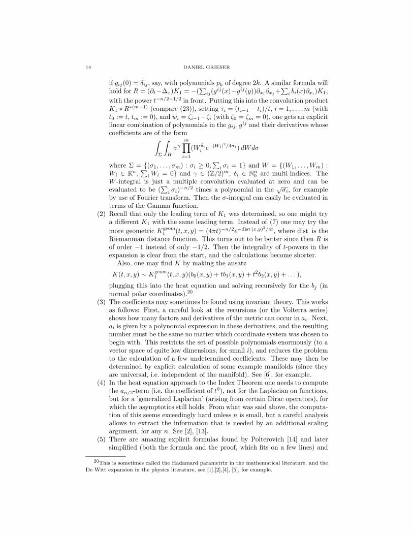
14 DANIEL GRIESER

if gij(0) = δij , say, with polynomials pk of degree 2k. A similar formula willhold for R = (∂t−∆x)K1 = −(

∑ij(g

ij(x)−gij(y))∂xi∂xj

+∑

i bi(x)∂xi)K1,

with the power t−n/2−1/2 in front. Putting this into the convolution productK1 ∗R∗(m−1) (compare (23)), setting τi = (ti−1 − ti)/t, i = 1, . . . ,m (witht0 := t, tm := 0), and wi = ζi−1−ζi (with ζ0 = ζm = 0), one gets an explicitlinear combination of polynomials in the gij , g

ij and their derivatives whosecoefficients are of the form∫

Σ

∫H

σγm∏

i=1

(W δii e

−|Wi|2/4σi) dWdσ

where Σ = {(σ1, . . . , σm) : σi ≥ 0,∑

i σi = 1} and W = {(W1, . . . ,Wm) :Wi ∈ Rn,

∑iWi = 0} and γ ∈ (Z/2)m, δi ∈ Nn

0 are multi-indices. TheW -integral is just a multiple convolution evaluated at zero and can beevaluated to be (

∑i σi)−n/2 times a polynomial in the

√σi, for example

by use of Fourier transform. Then the σ-integral can easily be evaluated interms of the Gamma function.

(2) Recall that only the leading term of K1 was determined, so one might trya different K1 with the same leading term. Instead of (7) one may try themore geometric Kgeom

1 (t, x, y) = (4πt)−n/2e−dist (x,y)2/4t, where dist is theRiemannian distance function. This turns out to be better since then R isof order −1 instead of only −1/2. Then the integrality of t-powers in theexpansion is clear from the start, and the calculations become shorter.

Also, one may find K by making the ansatz

K(t, x, y) ∼ Kgeom1 (t, x, y)(b0(x, y) + tb1(x, y) + t2b2(x, y) + . . . ),

plugging this into the heat equation and solving recursively for the bj (innormal polar coordinates).20

(3) The coefficients may sometimes be found using invariant theory. This worksas follows: First, a careful look at the recursions (or the Volterra series)shows how many factors and derivatives of the metric can occur in ai. Next,ai is given by a polynomial expression in these derivatives, and the resultingnumber must be the same no matter which coordinate system was chosen tobegin with. This restricts the set of possible polynomials enormously (to avector space of quite low dimensions, for small i), and reduces the problemto the calculation of a few undetermined coefficients. These may then bedetermined by explicit calculation of some example manifolds (since theyare universal, i.e. independent of the manifold). See [6], for example.

(4) In the heat equation approach to the Index Theorem one needs to computethe an/2-term (i.e. the coefficient of t0), not for the Laplacian on functions,but for a ’generalized Laplacian’ (arising from certain Dirac operators), forwhich the asymptotics still holds. From what was said above, the computa-tion of this seems exceedingly hard unless n is small, but a careful analysisallows to extract the information that is needed by an additional scalingargument, for any n. See [2], [13].

(5) There are amazing explicit formulas found by Polterovich [14] and latersimplified (both the formula and the proof, which fits on a few lines) and

20This is sometimes called the Hadamard parametrix in the mathematical literature, and the

De Witt expansion in the physics literature, see [1],[2],[4], [5], for example.

NOTES ON HEAT KERNEL ASYMPTOTICS 15

generalized by Weingart [15]:

ak(y) =k∑

l=0

(− 1

4

)l(k + n

2

k − l

) [(−1)k+l

(k + l)!∆k+l

x (1l!

dist2l(x, y) )]|x=y

.

(6) There are other approaches to the computation. See for example the book[10], which also contains many examples.

2.5.4. Generalization to other elliptic operators. If the Laplacian is replaced by anyelliptic differential operator P, of order d > 0, acting on a vector bundle, essentiallythe same procedure works to show the existence and uniqueness of a corresponding’heat kernel’, as long as the ’model solutions’ (generalizing (6)) are rapidly decayingoff the diagonal. Since these can be obtained using Fourier transform from theleading part of P , with coefficients frozen at y, this translates to a condition on theprincipal symbol of P 21. The minor adjustments are:

√t should be replaced by

t1/d everywhere. K takes values in homomorphisms from the fiber over y to thefiber over x, so the leading term has values in Endomorphisms of the fiber over y.In the uniqueness argument, the dual operator must be used.

21The condition is that all eigenvalues of the principal symbol (which takes values in endomor-

phisms of the bundle) have negative real part; sometimes this is called Petrovski-ellipticity.

16 DANIEL GRIESER

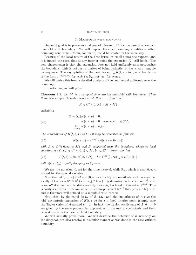
3. Manifolds with boundary

Our next goal is to prove an analogue of Theorem 1.1 for the case of a compactmanifold with boundary. We will impose Dirichlet boundary conditions; otherboundary conditions (Robin, Neumann) could be treated in the same way.

Because of the local nature of the heat kernel at small times one expects, andit is indeed the case, that at any interior point the expansion (2) still holds. Thenew phenomenon is that the expansion does not hold uniformly as x approachesthe boundary. This is not just a matter of being pedantic. It has a very tangibleconsequence: The asymptotics of the heat trace,

∫MK(t, x, x) dx, now has terms

of the form t−n/2+j/2 for each j ∈ N0, not just for even j.We will derive this from a detailed analysis of the heat kernel uniformly near the

boundary.In particular, we will prove:

Theorem 3.1. Let M be a compact Riemannian manifold with boundary. Thenthere is a unique Dirichlet heat kernel, that is, a function

K ∈ C∞((0,∞)×M ×M)

satisfying

(∂t −∆x)K(t, x, y) = 0,

K(t, x, y) = 0 whenever x ∈ ∂M,

limt→0+

K(t, x, y) = δy(x).(26)

The smoothness of K(t, x, x) as t→ 0 may be described as follows:

(27) K(t, x, x) = t−n/2 (A(t, x) +B(t, x))

with A ∈ C∞([0,∞) × M) and B supported near the boundary, where in localcoordinates (x′, xn) ∈ U ′ × [0, ε) ⊂M , U ′ ⊂ Rn−1 open, one has

(28) B(t, x) = b(t, x′, xn/√t), b ∈ C∞([0,∞)√t × U ′ × R+)

with b(t, x′, ξn) rapidly decaying as ξn →∞.

We use the notation [0,∞) for the time interval, while R+, which is also [0,∞),is used for the spacial variable xn.

Note that M2, [0,∞)×M and [0,∞)×U ′×R+ are manifolds with corners, i.e.locally of the form Rk

+×Rl (with k ≤ 2 here). By definition, a function on Rk+×Rl

is smooth if it can be extended smoothly to a neighborhood of this set in Rk+l. Thisis easily seen to be invariant under diffeomorphisms of Rk+l that preserve Rk

+ ×Rl

and is therefore well-defined on a manifold with corners.Note that, by the rapid decay of B, (27) and the smoothness of A give the

’old’ asymptotic expansion of K(t, x, x) for x a fixed interior point (simply takethe Taylor series of A around t = 0). In fact, the Taylor coefficients of A at t = 0are given by the same polynomial expressions in the metric coefficients and theirderivatives as in the case without boundary.

We will actually prove more: We will describe the behavior of K not only onthe diagonal, but also nearby, in a similar manner as was done in the case withoutboundary.

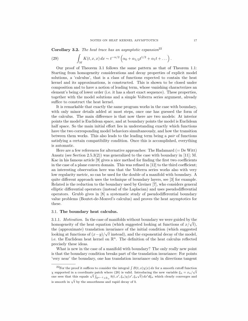
NOTES ON HEAT KERNEL ASYMPTOTICS 17

Corollary 3.2. The heat trace has an asymptotic expansion22

(29)∫

M

K(t, x, x) dx ∼ t−n/2(α0 + α1/2t

1/2 + α1t+ . . .).

Our proof of Theorem 3.1 follows the same pattern as that of Theorem 1.1:Starting from homogeneity considerations and decay properties of explicit modelsolutions, a ’calculus’, that is a class of functions expected to contain the heatkernel and its approximations, is constructed. This is shown to be closed undercomposition and to have a notion of leading term, whose vanishing characterizes anelement’s being of lower order (i.e. it has a short exact sequence). These properties,together with the model solutions and a simple Volterra series argument, alreadysuffice to construct the heat kernel.

It is remarkable that exactly the same program works in the case with boundary,with only minor details added at most steps, once one has guessed the form ofthe calculus. The main difference is that now there are two models: At interiorpoints the model is Euclidean space, and at boundary points the model is Euclideanhalf space. So the main initial effort lies in understanding exactly which functionshave the two corresponding model behaviors simultaneously, and how the transitionbetween them works. This also leads to the leading term being a pair of functionssatisfying a certain compatibility condition. Once this is accomplished, everythingis automatic.

Here are a few references for alternative approaches: The Hadamard (= De Witt)Ansatz (see Section 2.5.3(2)) was generalized to the case with boundary in [11]; M.Kac in his famous article [9] gives a nice method for finding the first two coefficientsin the case of a plane convex domain. This was refined in [12] to the third coefficient;an interesting observation here was that the Volterra series works also with verylow regularity metric, so can be used for the double of a manifold with boundary. Aquite different approach uses the technique of boundary layers, see [3] for example.Related is the reduction to the boundary used by Greiner [7], who considers generalelliptic differential operators (instead of the Laplacian) and uses pseudodifferentialoperators. Grubb gives in [8] a systematic study of pseudodifferential boundaryvalue problems (Boutet-de-Monvel’s calculus) and proves the heat asymptotics forthese.

3.1. The boundary heat calculus.

3.1.1. Motivation. In the case of manifolds without boundary we were guided by thehomogeneity of the heat equation (which suggested looking at functions of x/

√t),

the (approximate) translation invariance of the initial condition (which suggestedlooking at functions of (x−y)/

√t instead), and the exponential decay of the model,

i.e. the Euclidean heat kernel on Rn. The definition of the heat calculus reflectedprecisely these ideas.

What is new in the case of a manifold with boundary? The only really new pointis that the boundary condition breaks part of the translation invariance: For points’very near’ the boundary, one has translation invariance only in directions tangent

22For the proof it suffices to consider the integral∫B(t, x)χ(x) dx for a smooth cutoff function

χ supported in a coordinate patch where (28) is valid. Introducing the new variable ξn = xn/√t

one sees that this equals√t∫

Rn−1×R+b(t, x′, ξn)χ(x′, ξn

√t) dx′dξn which clearly converges and

is smooth in√t by the smoothness and rapid decay of b.

18 DANIEL GRIESER

to the boundary. This means that, at least near the boundary, we should expectthe heat kernel to be a function of t, (x′− y′)/

√t, xn/

√t and yn/

√t and y′, where

here and always we use coordinates near the boundary

(30) (x′, xn) ∈ U = U ′ × [0, ε) ⊂M, U ′ × {0} = U ∩ ∂M, U ′ ⊂ Rn−1.

This expectation is supported by the explicit formula for the Dirichlet heat kernelon the Euclidean half space Rn−1 × R+:

(31) E∂(t, x, y) = (4πt)−n/2(e−|x−y|2/4t − e−|x

∗−y|2/4t), x∗ := (x′,−xn),

which may be rewritten

(32) E∂(t, x, y) = (4πt)−n/2e−|X′|2/4

(e−(ξn−ηn)2/4 − e−(ξn+ηn)2/4

)where

(33) X ′ =x′ − y′√

t, ξn =

xn√t, ηn =

yn√t.

Apart from this new feature, we would like to proceed essentially as in thecase without boundary. That is, we would like to define a class of functions on(0,∞)×M2, to be called the boundary heat calculus, which:

• reflects the homogeneity and decay properties of the model heat kernels onRn−1 × R+ and on Rn,

• has a notion of ’order’,• has a notion of leading part, with a corresponding short exact sequence,

and• has a composition theorem.

One way to look at (31) is this: E∂ is the sum of a ’direct’ term, which equalsthe Rn heat kernel E, and a reflected term. The reflected term is chosen to satisfythe heat equation (with zero initial condition) and with boundary data preciselycancelling the restriction of the direct term to the boundary. From the principleof locality it is to be expected, and can be read off from formula (32), that thereflected term decays rapidly on the scale of

√t as x or y leaves the boundary. In

particular, E∂ reduces to E plus O(t∞) as soon as either x or y stays away a fixeddistance from the boundary.

In addition to this we will need to look at E∂ as one basic object, rather thanas the difference of two. This is imposed on us by our method: Only this allowsfor a reasonable notion of leading part. Also, it is motivated by the homogeneityconsiderations above23.

This motivates the following definition.

3.1.2. Definition of the calculus.

Definition 3.3. Let M be a manifold with boundary. The boundary heat calculus,denoted Ψα

H,∂(M), is, for each α ≤ 0, the space of functions A on (0,∞) ×M2

satisfying properties (a), (b) of Definition 2.1, property (c) for interior points p,and in addition:

23and by the expectation that only this changed perspective allows generalization to other

geometries, for example conical singularities where the reflection principle is not available.

NOTES ON HEAT KERNEL ASYMPTOTICS 19

(d) for each p ∈ ∂M there is a coordinate neighborhood as in (30) and functions

Adir ∈ C∞([0,∞)√t × Rn × U)(34)

Arefl, Abd ∈ C∞([0,∞)√t × Rn−1 × R2+ × U ′)(35)

so that for x, y ∈ U , t > 0 one has

A(t, x, y) = t−n+2

2 −α

(Adir(t,

x− y√t, y)− Arefl(t,

x′ − y′√t

,xn√t,yn√t, y′)

),

=: t−n+2

2 −αAbd(t,x′ − y′√

t,xn√t,yn√t, y′)

(36)

with rapid decay for Adir as in (10) and

(37) Arefl(t,X ′, ξn, ηn, y′) = O((ξn + ηn + |X ′|)−∞),

together with all derivatives, uniformly for bounded t.

Note that Arefl depends on the same number of variables as Adir (and as A), asit should.

One may be tempted to include the boundary condition in the calculus (A(t, x, y) =0 whenever x ∈ ∂M), but this is not a good idea since applying ∆x would get usout of the calculus.

Let us check that (d) implies (c) for y near an interior point of U : Simply setA(t,X, y) = Adir(t,X, y)− Arefl(t,X ′, Xn + yn/

√t, yn/

√t, y′), then (36) is exactly

(9), and smoothness at√t = 0 follows from yn > 0 and (37). Also, one sees that

(38) A = Adir for t = 0, yn > 0.

For future reference let us rewrite the second equality of (36) in rescaled coordi-nates:

(39) Abd(t,X ′, ξn, ηn, y′) = Adir(t,X ′, ξn − ηn, y

′, ηn

√t)− Arefl(t,X ′, ξn, ηn, y

′).

We need to define the ’leading term’. Recall that this must be done so thatthe vanishing of the leading term of an element of Ψα

H,∂ characterizes its being in

Ψα−1/2H,∂ .Looking at (36), we are led to:

Definition 3.4. Let A ∈ ΨαH,∂(M). Given coordinates in the interior of M , define

the interior leading term, Φintα (A) just like the leading term in Definition 2.2.

Given coordinates near the boundary as in Definition 3.3(d), define the boundaryleading term, Φbd

α (A), as the function(40)Φbd

α (A)(X ′, ξn, ηn, y′) = Abd(0, X ′, ξn, ηn, y

′) for X ′ ∈ Rn−1, ξn, ηn ∈ R+, y′ ∈ U ′.

Again, Abd is not defined uniquely by A, but still its values at t = 0 are, as canbe seen from simply rearranging (36) into

(41) Abd(t,X ′, ξn, ηn, y′) = t(n+2)/2+αA(t, y′ +X ′√t, ξn

√t, y′, ηn

√t).

Again, the highest priority is to analyze how these things depend on the choiceof coordinates.

20 DANIEL GRIESER

3.1.3. Coordinate invariance. We proceed similarly to the boundaryless case. Butfirst we need to define a bundle which will turn out to carry the boundary leadingpart. Define the vector bundle E → ∂M with fiber over a point p ∈ ∂M given by

Ep = (TpM × TpM)/Tp∂M, where(42)

u ∈ Tp∂M acts on (v, w) ∈ TpM × TpM as (u+ v, u+ w).(43)

(43) makes sense since Tp∂M ⊂ TpM naturally. Note that Ep has dimension n+1.One has a vector bundle map defined for p ∈ ∂M by

βp : Ep → TpM, [v, w] 7→ v − w,

with [v, w] denoting the equivalence class of the pair (v, w).Define the inward pointing part of E by

E+p = (T+

p M × T+p M)/Tp∂M,

where T+p M ⊂ TpM is the closed half space of vectors pointing into the interior of

M , or tangent to ∂M . Clearly, this makes sense since Tp∂M ⊂ T+p M , and E+

p isa conical subset 24 of Ep. Also, the total space E+ is a manifold with corners (ofcodimension two). So the space C∞S(fibers)(E

+) of smooth functions on E+ whichdecay rapidly in the fibers is well-defined. Then set

C∞bd(E+) := {φbd ∈ C∞(E+) :φbd = β∗φdir − φrefl for some

φdir ∈ C∞S(fibers)(T∂MM), φrefl ∈ C∞S(fibers)(E)}.

(44)

Given local coordinates on M near a boundary point, all of this looks as follows:Let (∂xi)i=1,...,n be the local frame on TM defined by the coordinates, and let(∂yi)i=1,...,n be a second copy of it (so the ∂xi , ∂yi are a local frame for TM ⊕TM).Then the collection (

12(∂xi − ∂yi)

)i=1,...,n−1

, ∂xn , ∂yn

may be taken as frame in E. We denote the corresponding coordinates by X ′ =(X1, . . . , Xn−1), ξn, ηn. Clearly, E+ is characterized by ξn ≥ 0, ηn ≥ 0. With thesecoordinates on E, and with natural coordinates on TM , one has β(X ′, ξn, ηn, y

′) =(X ′, ξn − ηn, y

′). A function φbd on E+ is in C∞bd(E+) iff, in coordinates, it is thesum of a function in the variables X ′, ξn − ηn, y

′, rapidly decaying in (X ′, ξn − ηn),and a function in X ′, ξn, ηn, y

′, rapidly decaying in (X ′, ξn, ηn). Roughly speaking,this means that rapid decay is not required when going off to infinity along the’diagonal’ in E+. This corresponds precisely to the decomposition in (39).

Lemma 3.5. (a) If condition (d) in Definition 3.3 holds in one coordinatesystem then it holds in any.

(b) The interior leading term Φintα (A) is defined invariantly as a function on

the tangent bundle which is smooth up to the boundary and rapidly decayingin the fiber direction:

(45) Φintα (A) ∈ C∞S(fibers)(TM).

24that is, α ∈ E+p , r > 0 imply rα ∈ E+

p

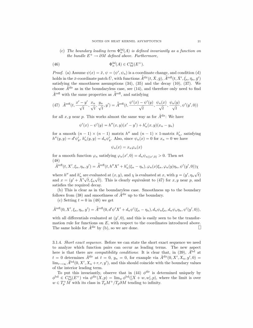
NOTES ON HEAT KERNEL ASYMPTOTICS 21

(c) The boundary leading term Φbdα (A) is defined invariantly as a function on

the bundle E+ → ∂M defined above. Furthermore,

(46) Φbdα (A) ∈ C∞bd (E+).

Proof. (a) Assume ψ(x) = x, ψ = (ψ′, ψn) is a coordinate change, and condition (d)holds in the x-coordinate patch U , with functions ¯Adir(t, X, y), ¯Arefl(t, X ′, ξn, ηn, y

′)satisfying the smoothness assumptions (34), (35) and the decay (10), (37). Wechoose Adir as in the boundaryless case, see (14), and therefore only need to findArefl with the same properties as ¯Arefl, and satisfying

(47) Arefl(t,x′ − y′√

t,xn√t,yn√t, y′) = ¯Arefl(t,

ψ′(x)− ψ′(y)√t

,ψn(x)√

t,ψn(y)√

t, ψ′(y′, 0))

for all x, y near p. This works almost the same way as for Adir: We have

ψ′(x)− ψ′(y) = h′′(x, y)(x′ − y′) + h′n(x, y)(xn − yn)

for a smooth (n − 1) × (n − 1) matrix h′′ and (n − 1) × 1-matrix h′n, satisfyingh′′(y, y) = d′ψ′y, h′n(y, y) = dnψ

′y. Also, since ψn(x) = 0 for xn = 0 we have

ψn(x) = xnϕn(x)

for a smooth function ϕn satisfying ϕn(x′, 0) = dnψn|(x′,0) > 0. Then set(48)Arefl(t,X ′, ξn, ηn, y

′) = ¯Arefl(t, h′′X ′ + h′n(ξn − ηn), ϕn(x)ξn, ϕn(y)ηn, ψ′(y′, 0))χ

where h′′ and h′n are evaluated at (x, y), and χ is evaluated at x, with y = (y′, ηn

√t)

and x = (y′ + X ′√t, ξn√t). This is clearly equivalent to (47) for x, y near p, and

satisfies the required decay.(b) This is clear as in the boundaryless case. Smoothness up to the boundary

follows from (38) and smoothness of Adir up to the boundary.(c) Setting t = 0 in (48) we get

Arefl(0, X ′, ξn, ηn, y′) = ¯Arefl(0, d′ψ′X ′ + dnψ

′(ξn − ηn), dnψnξn, dnψnηn, ψ′(y′, 0)),

with all differentials evaluated at (y′, 0), and this is easily seen to be the transfor-mation rule for functions on E, with respect to the coordinates introduced above.The same holds for Adir by (b), so we are done.

3.1.4. Short exact sequence. Before we can state the short exact sequence we needto analyze which function pairs can occur as leading terms. The new aspecthere is that there are compatibility conditions: It is clear that, in (39), Abd att = 0 determines Adir at t = 0, yn = 0, for example via Adir(0, X ′, Xn, y

′, 0) =limr→∞ Abd(0, X ′, Xn + r, r, y′), and this should coincide with the boundary valuesof the interior leading term.

To put this invariantly, observe that in (44) φdir is determined uniquely byφbd ∈ C∞bd(E+) via φdir(X, p) = limw φ

bd([X + w,w], p), where the limit is overw ∈ T+

p M with its class in TpM+/Tp∂M tending to infinity.

22 DANIEL GRIESER

Definition 3.6. The space of leading terms, C∞Φ,∂(M), is the subspace of C∞S(fibers)(TM)×C∞bd (E+) given by pairs25 (φint, φbd) satisfying

(49) φint|T∂M M = φdir

where φdir is determined by φbd as explained above.

Lemma 3.7. The sequence

0 → Ψα−1/2H,∂ (M) → Ψα

H,∂(M) Φα→ C∞Φ,∂(M) → 0

is exact.

Proof. This is clear except possibly at C∞Φ,∂(M). To prove surjectivity of Φα we mayclearly work locally near the boundary, so suppose we have functions φint, φbd =β∗φdir − φrefl satisfying (49). Then set, locally,

A(t, x, y) = t−(n+2)/2−α

(φint(

x− y√t, y)− φrefl(

x′ − y′√t

,xn√t,yn√t, y′)

).

This has interior leading part φint since φrefl is rapidly decaying in X ′, ξn, ηn, andhas boundary leading part φbd because of (49).

3.1.5. Composition.

Proposition 3.8. Let A ∈ ΨαH,∂(M), B ∈ Ψβ

H,∂(M), with α, β < 0, and assumeM is compact. Then A ∗ B is defined and lies in Ψα+β

H,∂ (M). The interior leadingterm is calculated as in (16), and the boundary leading terms satisfy

(50) (a ∗ b)bd(X ′, ξn, ηn, p) =∫ 1

0

∫Rn−1

∫R+

(1− σ)−(n+2)/2−ασ−(n+2)/2−β

abd(

(X ′ − Z ′, ξn, ζn)√1− σ

, p

)bbd

((Z ′, ζn, ηn)√

σ, p

)dζndZ

′dσ.

(The formula for the leading term will not be used.)

Proof. As in the proof of the case without boundary, it is enough to consider x, y in acoordinate patch U . Furthermore, we may assume that U = U ′×[0, ε) is a boundarycoordinate patch, where A,B have representations as in (36), and to consider thelocalized integral (17). We replace the integration variables by σ = s/t, Z ′ =(z−y)/

√t, ζn = zn/

√t and introduce new variables X ′ = (x′−y′)/

√t, ξn = xn/

√t,

ηn/√t instead of x′. xn, yn. Then (17) becomes t−(n+2)/2−α−βCbd(t,X ′, ξn, ηn, y

′)where Cbd(t,X ′, ξn, ηn, y

′) equals

(51)∫ 1

0

∫Rn−1

∫R+

dζn dZ′ dσ(1− σ)−(n+2)/2−ασ−(n+2)/2−β ·

Abd(t(1−σ),(X ′ − Z ′, ξn, ζn)√

1− σ, y′+Z ′

√t)Bbd(tσ,

(Z ′, ζn, ηn)√σ

, y′)χ(y′+Z ′√t, ξn

√t).

We need to check convergence and rapid decay properties for each of the fourterms arising from splitting up Abd, Bbd as sums of direct and reflected terms (asin (39)). The product of direct terms is done as in the case without boundary.

25that the leading term is a pair of functions corresponds to the two symbol levels in the

Boutet-de-Monvel calculus, see [8]

NOTES ON HEAT KERNEL ASYMPTOTICS 23

We claim that the other three terms are all in C∞S(fibers)(E+), that is, they decay

rapidly in all the variables X ′, ξn, ηn. For example, let us look at the direct termAdir and the reflected term Brefl. In the region σ ≤ 1/2 introduce the variablesW ′ = Z ′/

√σ for Z ′ and ρn = ζn/

√σ for ζn. Then the power of σ is −1− β, so the

integral converges since β < 0, and the integrand of the dρndZ′ integral is bounded

by (||X ′| − |W ′|| + |ξn − ρn|)−N (|W ′| + ρn + ηn/√σ)−N for any N , from which

convergence and rapid decay of the integral is easily seen. Derivatives, the regionσ ≥ 1/2 and the other cases are treated similarly.

Formula (50) follows immediately from (51).

We also have the analogue of Proposition 2.7:

Proposition 3.9. (1) Let A ∈ ΨαH,∂(M), α ≤ −1. Then (∂t − ∆x)A ∈

Ψα+1H,∂ (M).

(2) The interior leading terms of A and R = (∂t−∆x)A are related as in (19),and the boundary leading terms abd = Φbd

α (A) and rbd = Φbdα+1(R) satisfy

(52) rbd(X ′, ξn, ηn, p) = [−n+ 22

− α− 12X ′∂′X

− 12ξn∂ξn

− 12ηn∂ηn

−∆0,pX′,ξn

]abd(X ′, ξn, ηn, p).

Here, ∆0,pX′,ξn

=∑

ij gij(p)∂Xi

∂Xj(with Xn replaced by ξn).

Again, formula (52) will not be used directly.

Proof. In the interior, this follows from Proposition 2.7. Near a boundary pointwrite A(t, x, y) = t−lAbd(t, x′−y′√

t, xn√

t, yn√

t, y′), l = n+2

2 +α, then the calculation is thesame as in the case without boundary, except thatXn is replaced by ξn in the formu-las, in the t-derivative one has an extra term −t−l yn

2t3/2 ∂ηnAbd = −t−l−1 1

2ηn∂ηnAbd,

and in the computation of ∆xA there is an additional contribution to the re-mainder R2 from writing gij(y) = gij(y′, 0) + hij

1 (y)yn, where the second termis√t hij

1 (y′,√tηn)ηn and thus lower order.

3.1.6. Boundary conditions. Let

ΨαH,Dir(M) = {A ∈ Ψα

H,∂(M) : A(t, x, y) = 0 whenever x ∈ ∂M}.

The following lemma is obvious:

Lemma 3.10. (a) Let A ∈ ΨαH,Dir, B ∈ Ψβ

H,∂ , where α, β < 0. Then A ∗ B ∈Ψα+β

H,Dir.(b) There is a short exact sequence for Ψα

H,Dir, with boundary leading partsvanishing at the ’left’ boundary (ξn = 0) of E+.

3.1.7. Evaluation at t = 0. Lemma 2.8 carries over directly, mutatis mutandis; thatis, in (20) one uses the interior leading part of A, and the boundary leading partplays no role.

24 DANIEL GRIESER

3.2. The Volterra series. We restate Proposition 2.10 in the present context:

Proposition 3.11. Assume K1 ∈ Ψ−1H,∂ satisfies

(∂t −∆x)K1 = R ∈ Ψ−1/2H,∂ ,

K1(t, x, y) = 0 whenever x ∈ ∂M, (soK1 ∈ Ψ−1H,Dir)

limt→0+

K1(t, x, y) = δy(x).(53)

(a) Then

(54) K := K1 −K1 ∗R+K1 ∗R ∗R− . . .

converges in C∞((0,∞)×M2), and K ∈ Ψ−1H,Dir(M).

(b) K is a Dirichlet heat kernel, that is, it satisfies (26).(c) The series (54) is an asymptotic series as t→ 0. More precisely, K1∗R∗N ∈

Ψ−1−N/2H,Dir (M).

The proof carries over from Proposition 2.10 with almost no changes. Only inthe last sentence in its proof one should use, near the boundary, a cutoff χ(x)χ(y) =χ(y′ +X ′√t, ξn

√t)χ(y′, ηn

√t) instead, on whose support |X ′|+ ξn + ηn ≤ Ct−1/2,

which gives the required exponential decay in the reflected term.

3.3. Construction of the heat kernel.

Theorem 3.12. Let M be a compact Riemannian manifold with boundary. Thenthere is a unique Dirichlet heat kernel K, and it lies in Ψ−1

H,∂(M).Furthermore, K may be split K = Kint+Kbd where tn/2Kint(t, x, x) ∈ C∞([0,∞)×

M) and Kbd(t, x, y) = O([d(x)/√t + d(y)/

√t]−∞), with d(x) the distance of x to

the boundary.

Proof. After all this preparation, this works just the same as in the case withoutboundary, except that the initial step is modified since there are two models.

Define (φint, φbd) ∈ C∞Φ,∂(M) by

φint(X, p) = (4π)n/2e−|X|2g(p)/4, p ∈M

φbd([v, w], p) = (4π)n/2(e−|v−w|2g(p)/4 − e−|v−w∗|2g(p)/4

), p ∈ ∂M

where the ’reflected’ vector w∗ of w ∈ TpM , for p ∈ ∂M , is defined as follows:Write w = wbd + wn with wbd tangential to the boundary and wn normal to it,with respect to the metric g(p); then w∗ := wbd − wn. 26 With this definition itis clear that |w| = |w∗|, so φbd satisfies the boundary condition in Lemma 3.10(b).Also, it is clear that φint, φbd satisfy the compatibility condition (49), so there isK1 ∈ Ψ−1

H,Dir with Φ−1(K1) = (φint, φbd).

26A little care is needed here: It would not work to choose any boundary adapted coordinates

(as before) and then, with w = (η′, ηn), set w∗ = (η′,−ηn), since the ’cross terms’ in |v−w∗ |2g , of

the form ginXi(ξn + ηn) with i ≤ n− 1 would not equal the corresponding terms ginXi(ξn − ηn)in |v − w|2 at ξn = 0, so the boundary condition would be violated by φbd unless gin = 0 for all

i ≤ n − 1. Therefore, only coordinates in which the xn direction is orthogonal to the tangential

directions can be used here, and our definition reflects precisely this, in a coordinate-free way.(Such choice of coordinates, called ’coordinates normal with respect to the boundary’ exist, butare not needed here.)

NOTES ON HEAT KERNEL ASYMPTOTICS 25

By Proposition 3.9 the remainder R = (∂t − ∆x)K1 is in Ψ0H,∂ with leading

term27 Φ0(R) = 0, so actually R ∈ Ψ−1/2H,∂ , and then the Volterra series gives a heat

kernel. Uniqueness can be proved in the same way as before.Note that K(t, x, y) = 0 for y ∈ ∂M also since this is true for K1, hence for R,

hence for K.The last claim is clear from the definition of ΨH,∂ , except for the smoothness of

K int(t, x, x) with respect to t (rather than√t). The latter follows in the same way

as the corresponding statement in the case without boundary, see the discussionafter (24).

27again, this could be computed from formula (52), or concluded directly from the fact thatthis formula says that the leading part can be computed by freezing coefficients and forgettinglower order terms.

26 DANIEL GRIESER

References

[1] Marcel Berger, Paul Gauduchon, and Edmond Mazet. Le spectre d’une variete riemannienne.Lecture Notes in Mathematics, Vol. 194. Springer-Verlag, Berlin, 1971.

[2] N. Berline, E. Getzler, and M. Vergne. Heat Kernels and Dirac Operators, volume 298 of

Grundlehren der mathematischen Wissenschaften. Springer–Verlag, Berlin, Heidelberg, NewYork, 1992.

[3] M. Bordag, D. Vassilevich, H. Falomir, and E. M. Santangelo. Multiple reflection expansion

and heat kernel coefficients. Phys. Rev. D (3), 64(4):045017, 11, 2001.[4] Isaac Chavel. Eigenvalues in Riemannian geometry, volume 115 of Pure and Applied Math-

ematics. Academic Press Inc., Orlando, FL, 1984. Including a chapter by Burton Randol,With an appendix by Jozef Dodziuk.

[5] Bryce S. DeWitt. Dynamical theory of groups and fields. Gordon and Breach Science Pub-

lishers, New York, 1965.[6] Peter B. Gilkey. Invariance theory, the heat-equation, and the Atiyah-Singer index theorem.

Studies in Advanced Mathematics. CRC Press, Boca Raton, 2 edition, 1995.

[7] Peter Greiner. An asymptotic expansion for the heat equation. Arch. Rational Mech. Anal.,41:163–218, 1971.

[8] Gerd Grubb. Functional calculus of pseudodifferential boundary problems, volume 65 of

Progress in Mathematics. Birkhauser Boston Inc., Boston, MA, second edition, 1996.[9] M. Kac. Can one hear the shape of a drum? Am. Math. Mon., Part II, 73:1–23, April 1966.

[10] Klaus Kirsten. Spectral functions in mathematics and physics. Chapman and Hall/CRC,

Boca Raton, Fla., 2002.[11] D. M. McAvity and H. Osborn. A DeWitt expansion of the heat kernel for manifolds with a

boundary. Classical Quantum Gravity, 8(4):603–638, 1991. Errata: vol. 9, 1992, p. 317.[12] H. P. McKean, Jr. and I. M. Singer. Curvature and the eigenvalues of the Laplacian. J.

Differential Geometry, 1(1):43–69, 1967.

[13] Richard B. Melrose. The Atiyah-Patodi-Singer index theorem. A. K. Peters, Ltd., Boston,Mass., 1993.

[14] Iosif Polterovich. Heat invariants of Riemannian manifolds. Israel J. Math., 119:239–252,

2000.[15] Gregor Weingart. A characterization of the heat kernel coefficients. Preprint,

http://arXiv.org/abs/math.DG/0105144, 2001.