Notes from Survival Analysis

Cambridge Part III Mathematical Tripos 2012-2013

Lecturer: Peter Treasure

Vivak Patel

March 23, 2013

1

Contents

1 Introduction, Censoring and Hazard 41.1 Introduction . . . . . . . . . . . . . . . . . . . . . . . . . . . . . . 41.2 Censoring . . . . . . . . . . . . . . . . . . . . . . . . . . . . . . . 41.3 Important Distributions . . . . . . . . . . . . . . . . . . . . . . . 51.4 Notation . . . . . . . . . . . . . . . . . . . . . . . . . . . . . . . . 51.5 Likelihood Function in Survival Analysis . . . . . . . . . . . . . . 6

2 Non- & Semi-parametric Inference & Testing 72.1 Kaplan-Meier Estimation . . . . . . . . . . . . . . . . . . . . . . 7

2.1.1 Introduction . . . . . . . . . . . . . . . . . . . . . . . . . 72.1.2 Estimators . . . . . . . . . . . . . . . . . . . . . . . . . . 72.1.3 Properties . . . . . . . . . . . . . . . . . . . . . . . . . . . 82.1.4 Profile Likelihood Curve for Confidence Intervals . . . . . 9

2.2 Proportional Hazards Modelling (Estimation) . . . . . . . . . . . 92.2.1 Introduction . . . . . . . . . . . . . . . . . . . . . . . . . 92.2.2 Partial Likelihood Functions . . . . . . . . . . . . . . . . 102.2.3 Estimator . . . . . . . . . . . . . . . . . . . . . . . . . . . 102.2.4 Censoring . . . . . . . . . . . . . . . . . . . . . . . . . . . 102.2.5 Ties . . . . . . . . . . . . . . . . . . . . . . . . . . . . . . 11

2.3 Counting Processes & Nelson-Aalen Estimator . . . . . . . . . . 112.3.1 Counting Process . . . . . . . . . . . . . . . . . . . . . . . 112.3.2 Counting Process in Survival Analysis . . . . . . . . . . . 122.3.3 General Estimator . . . . . . . . . . . . . . . . . . . . . . 122.3.4 Nelson-Aalen Estmator . . . . . . . . . . . . . . . . . . . 12

2.4 Log-Rank Test . . . . . . . . . . . . . . . . . . . . . . . . . . . . 132.4.1 Introduction . . . . . . . . . . . . . . . . . . . . . . . . . 132.4.2 Test . . . . . . . . . . . . . . . . . . . . . . . . . . . . . . 142.4.3 Stratification . . . . . . . . . . . . . . . . . . . . . . . . . 142.4.4 Relative Risk . . . . . . . . . . . . . . . . . . . . . . . . . 14

2.5 Model Checking . . . . . . . . . . . . . . . . . . . . . . . . . . . . 152.5.1 General Model Checking and Survival Analysis . . . . . . 152.5.2 Cox-Snell Residuals . . . . . . . . . . . . . . . . . . . . . 152.5.3 Cox-Snell Residuals and Censoring . . . . . . . . . . . . . 152.5.4 Martingale Residuals . . . . . . . . . . . . . . . . . . . . . 16

3 Advanced/Assorted Topics 163.1 Relative Survival Modelling (Estimation) . . . . . . . . . . . . . 16

3.1.1 Introduction & Motivation . . . . . . . . . . . . . . . . . 163.1.2 Parametric Likelihood Based Estimation . . . . . . . . . . 173.1.3 Nonparametric Counting Process Estimation . . . . . . . 18

3.2 Multiple Events Analysis: Marginal Modelling (Estimation) . . . 183.2.1 Introduction . . . . . . . . . . . . . . . . . . . . . . . . . 183.2.2 Jack-Knife . . . . . . . . . . . . . . . . . . . . . . . . . . . 193.2.3 Estimators . . . . . . . . . . . . . . . . . . . . . . . . . . 193.2.4 Generic Data Structure . . . . . . . . . . . . . . . . . . . 20

3.3 Frailty (Estimation) . . . . . . . . . . . . . . . . . . . . . . . . . 213.3.1 Introduction . . . . . . . . . . . . . . . . . . . . . . . . . 213.3.2 Proportional Frailty Model Estimator . . . . . . . . . . . 21

2

3.3.3 Influence of Unknown Variables in Proportional HazardsModel . . . . . . . . . . . . . . . . . . . . . . . . . . . . . 22

3.3.4 Inference of Frailty Variable . . . . . . . . . . . . . . . . . 233.4 Cure (Estimation) . . . . . . . . . . . . . . . . . . . . . . . . . . 23

3.4.1 Introduction . . . . . . . . . . . . . . . . . . . . . . . . . 233.4.2 Simple Model . . . . . . . . . . . . . . . . . . . . . . . . . 243.4.3 Extensions to Simple Model . . . . . . . . . . . . . . . . . 243.4.4 Expectation Maximisation . . . . . . . . . . . . . . . . . . 25

3.5 Empirical Likelihood . . . . . . . . . . . . . . . . . . . . . . . . . 253.5.1 Introduction . . . . . . . . . . . . . . . . . . . . . . . . . 253.5.2 Derivation of Kaplan-Meier . . . . . . . . . . . . . . . . . 263.5.3 Constrained Maximisation for Interval Estimation . . . . 27

3.6 Schoenfeld Residuals (Model Checking) . . . . . . . . . . . . . . 273.6.1 Introduction . . . . . . . . . . . . . . . . . . . . . . . . . 273.6.2 Schoenfeld Residual and Applications . . . . . . . . . . . 28

3.7 Planning Experiments: Determining size of a Study . . . . . . . 293.7.1 Introduction . . . . . . . . . . . . . . . . . . . . . . . . . 293.7.2 Sample Size Inequality . . . . . . . . . . . . . . . . . . . . 293.7.3 Parameters under H0 . . . . . . . . . . . . . . . . . . . . 303.7.4 Parameters under H1 . . . . . . . . . . . . . . . . . . . . 303.7.5 Sample Size . . . . . . . . . . . . . . . . . . . . . . . . . . 31

A Likelihood Tests and Properties 32

3

1 Introduction, Censoring and Hazard

1.1 Introduction

1. Aliases of Survival Analysis

(a) In medicine: Survival Analysis

(b) In engineering: Failure-time analysis

(c) In general: Time-to-event Analysis

2. Framework

(a) Scale: we need a scale to measure the duration of some event

(b) Start Event: a clearly defined event when we start measuring withthe scale

(c) Event: A clearly defined event of interest

Definition 1.1. The time-to-event, T , is a random variable thatmeasures the duration between the start event and the event. T ≥ 0and T = 0 at the start event.

3. Properties

(a) Generally, the scale is continuous, but is sometimes treated as discretefor convenience

(b) Also, scale is usually time, but could be something that is appropriate(e.g. miles)

(c) The scale flows left to right, so if an individual makes it to some t2which is greater than t1, then the individual has made it past t1

1.2 Censoring

Censoring occurs when we are unable to collect a complete set of data for asubject (i.e. we cannot record the time-to-event since the person drops out ofthe study, dies, the study ends etc.). It is impossible to avoid, so we mustunderstand it and model it.

Definition 1.2. 1. Censoring occurs when we have incomplete informationabout the time-to-event.

2. Time-to-censoring: C, is the duration between the start event and censor-ing

3. Right censoring: censoring which occurs before the event and after censor-ing the event has occurred but no information is collected

4. Uninformative Censoring: the act of censoring provides no informationabout the event time T

Remark 1.1. If censoring is informative, then we must model it as a randomevent C, which complicates our analysis. It is sufficient to show that if censoringis stochastically independent of T , then C is uninformative.

4

Example 1.1. Suppose we are doing a clinical trial of a drug and our eventoccurs when the subject experiences symptom relief.

1. If censoring occurs because the trial is stopped according to a plan, thenthis is uninformative censoring for individuals who have not yet had anevent.

2. If censoring occurs because an individual leaves the study owing to intoler-able side effects, this can be informative censoring because the side-effectsindicate that the drug is in effect and could relieve the individual’s symp-toms.

1.3 Important Distributions

Definition 1.3. Let T be a time-to-event random variable.

1. Survivor Function: F (t) = P[T > t]

2. Distribution Function: f(t) = −F ′(t) or F (t) =∫∞tf(s)ds

3. Hazard Function: the event rate at a time t conditioned upon observing

time t without an event occurring: h(t) = f(t)F (t)

4. Integrated Hazard Function:

(a) H(t) =∫ t0h(s)ds

(b) H(t) = − log[F (t)] or F (t) = exp[−H(t)]

Example 1.2. We consider the exponential family:

1. Suppose F (t) is a non-negative, decreasing function on [0,∞) with F (0) ≤1. The exponential survivor function is F (t) = exp[−θt] for θ > 0

2. Suppose h(t) is any non-negative function on [0,∞) such as h(t) = θ.Then, by definition: H(t) = θt and F (t) = exp[−θt]

Definition 1.4. Families of Distributions:

1. Accelerated Life Family: if F is a survivor function and λ > 0, F (tλ)defines an accelerated life family of distributions.

2. Proportional Hazard Family: if F is a survivor function and k > 0, thenF (t)k = exp(kH(t)) defines a proportional hazards family of distributions.

1.4 Notation

1. Let Ti be the time to event for an individual i

2. Let Ci be the time to censoring for an individual i

3. Let vi be the visibility for an individual i. vi = 1[Ti ≤ Ci]. It is 1 if wesee an event, 0 if the individual is censored.

4. Let Xi = min(Ci, Ti).

Note 1.1. There is a strict inequality for vi = 0, i.e. Ci < Ti. If anindividual is censored at time t we can either observe an event at time tor we do not (Ti > Ci)

5

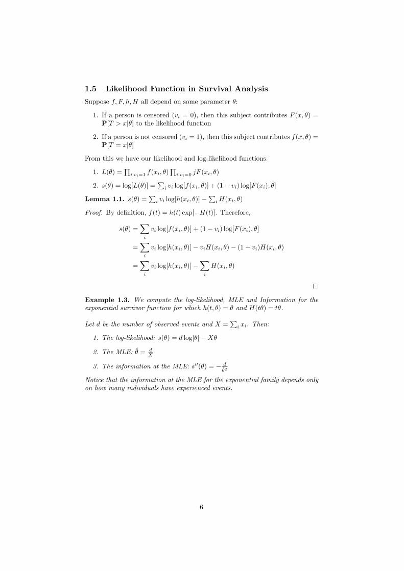
1.5 Likelihood Function in Survival Analysis

Suppose f, F, h,H all depend on some parameter θ:

1. If a person is censored (vi = 0), then this subject contributes F (x, θ) =P[T > x|θ] to the likelihood function

2. If a person is not censored (vi = 1), then this subject contributes f(x, θ) =P[T = x|θ]

From this we have our likelihood and log-likelihood functions:

1. L(θ) =∏i:vi=1 f(xi, θ)

∏i:vi=0 jF (xi, θ)

2. s(θ) = log[L(θ)] =∑i vi log[f(xi, θ)] + (1− vi) log[F (xi), θ]

Lemma 1.1. s(θ) =∑i vi log[h(xi, θ)]−

∑iH(xi, θ)

Proof. By definition, f(t) = h(t) exp[−H(t)]. Therefore,

s(θ) =∑i

vi log[f(xi, θ)] + (1− vi) log[F (xi), θ]

=∑i

vi log[h(xi, θ)]− viH(xi, θ)− (1− vi)H(xi, θ)

=∑i

vi log[h(xi, θ)]−∑i

H(xi, θ)

Example 1.3. We compute the log-likelihood, MLE and Information for theexponential survivor function for which h(t, θ) = θ and H(tθ) = tθ.

Let d be the number of observed events and X =∑i xi. Then:

1. The log-likelihood: s(θ) = d log[θ]−Xθ

2. The MLE: θ = dX

3. The information at the MLE: s′′(θ) = − dθ2

Notice that the information at the MLE for the exponential family depends onlyon how many individuals have experienced events.

6

2 Non- & Semi-parametric Inference & Testing

In parametric inference we assume some structure about an unknown parameterθ (e.g. we may know the dimension of the parameter space). In nonparametricinference, we assume θ is infinite dimensional or that the number of dimensionsincreases with each observed event.

Overview:

1. Kaplan-Meier Estimation, Proportional Hazards Modelling and CountingProcesses (Nelson-Aalen Estimator) are methods for estimating the sur-vivor or hazard functions

2. Log-rank test is a method for determining if two hazard functions aredifferent

3. Model checking is about methods used to evaluate and improve our models

2.1 Kaplan-Meier Estimation

2.1.1 Introduction

1. Purpose: A non-parametric method for estimating the survivor function

2. Assumptions: we assume that events only occur at discrete times

3. Notation

(a) We assume a fixed, sorted set of finite potential event times {a0 <a1 < · · · < ag}.

(b) Let the number of individuals at risk (still without an event and notcensored) at time aj be rj

(c) The number of events at time rj is dj ∼ Binomial(rj , qj) where qj =P[event at aj | at risk at aj ]

2.1.2 Estimators

The Kaplan Meier Estimator is F (t) =∏j:aj≤t(1− qj) =

∏j:aj≤t(1−

djrj

)

Derivation 2.1. We derive the Kaplan-Meier Estimator

1. Note that there are no event gaps, i.e. P[T ≥ aj ] = P[T > aj−1]

2. Secondly, P[T > aj |T ≥ aj ] = P[no event at aj |at risk at aj ] = 1− qj

3. Since qj is conditional on rj, which accounts for censored data, the cen-soring is uninformative

4. Suppose aj−1 ≤ t < aj, then

F (t) = P[T > t] = P[T > a0]P[T > a1|T ≥ a1] · · ·P[T > aj |T ≥ aj ]

5. We estimate qj with qj =djrj

7

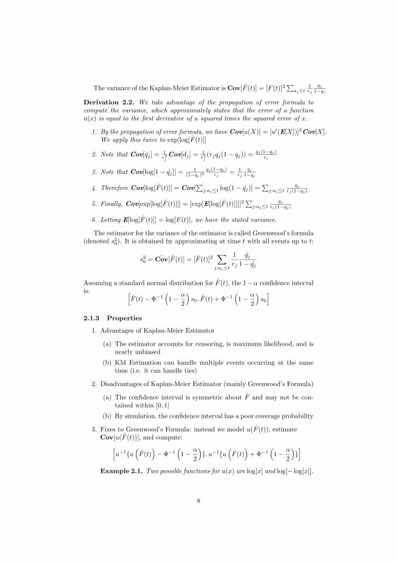
The variance of the Kaplan-Meier Estimator is Cov[F (t)] = [F (t)]2∑aj≤t

1rj

qj1−qj

Derivation 2.2. We take advantage of the propagation of error formula tocompute the variance, which approximately states that the error of a functionu(x) is equal to the first derivative of u squared times the squared error of x.

1. By the propagation of error formula, we have Cov[u(X)] = [u′(E[X])]2Cov[X].We apply this twice to exp[log[F (t)]]

2. Note that Cov[qj ] = 1r2jCov[dj ] = 1

r2j(rjqj(1− qj)) =

qj(1−qj)rj

3. Note that Cov[log[1− qj ]] = 1(1−qj)2

qj(1−qj)rj

= 1rj

qj1−qj

4. Therefore Cov[log[F (t)]] = Cov[∑j:aj≤t log(1− qj)] =

∑j:aj≤t

qjrj(1−qj)

5. Finally, Cov[exp[log[F (t)]]] = [exp[E[log[F (t)]]]]2∑j:aj≤t

qjrj(1−qj)

6. Letting E[log[F (t)]] = log[F (t)], we have the stated variance.

The estimator for the variance of the estimator is called Greenwood’s formula(denoted s20). It is obtained by approximating at time t with all events up to t:

s20 = ˆCov[F (t)] = [F (t)]2∑j:aj≤t

1

rj

qj1− qj

Assuming a standard normal distribution for F (t), the 1−α confidence intervalis: [

F (t)− Φ−1(

1− α

2

)s0, F (t) + Φ−1

(1− α

2

)s0

]2.1.3 Properties

1. Advantages of Kaplan-Meier Estimator

(a) The estimator accounts for censoring, is maximum likelihood, and isnearly unbiased

(b) KM Estimation can handle multiple events occurring at the sametime (i.e. it can handle ties)

2. Disadvantages of Kaplan-Meier Estimator (mainly Greenwood’s Formula)

(a) The confidence interval is symmetric about F and may not be con-tained within [0, 1]

(b) By simulation, the confidence interval has a poor coverage probability

3. Fixes to Greenwood’s Formula: instead we model u(F (t)), estimateCov[u(F (t))], and compute:[

u−1{u(F (t)

)− Φ−1

(1− α

2

)}, u−1{u

(F (t)

)+ Φ−1

(1− α

2

)}]

Example 2.1. Two possible functions for u(x) are log[x] and log[− log[x]].

8

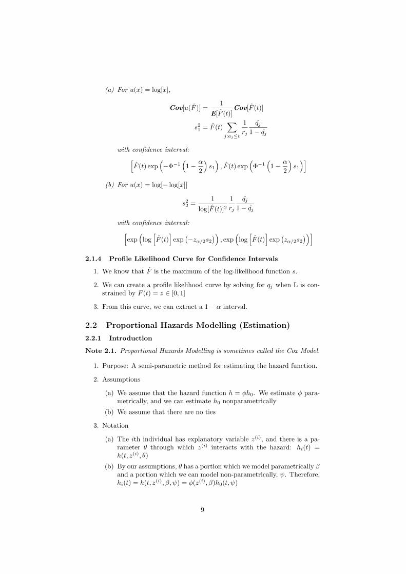
(a) For u(x) = log[x],

Cov[u(F )] =1

E[F (t)]Cov[F (t)]

s21 = F (t)∑j:aj≤t

1

rj

qj1− qj

with confidence interval:[F (t) exp

(−Φ−1

(1− α

2

)s1

), F (t) exp

(Φ−1

(1− α

2

)s1

)](b) For u(x) = log[− log[x]]

s22 =1

log[F (t)]21

rj

qj1− qj

with confidence interval:[exp

(log[F (t)

]exp

(−zα/2s2

)), exp

(log[F (t)

]exp

(zα/2s2

))]2.1.4 Profile Likelihood Curve for Confidence Intervals

1. We know that F is the maximum of the log-likelihood function s.

2. We can create a profile likelihood curve by solving for qj when L is con-strained by F (t) = z ∈ [0, 1]

3. From this curve, we can extract a 1− α interval.

2.2 Proportional Hazards Modelling (Estimation)

2.2.1 Introduction

Note 2.1. Proportional Hazards Modelling is sometimes called the Cox Model.

1. Purpose: A semi-parametric method for estimating the hazard function.

2. Assumptions

(a) We assume that the hazard function h = φh0. We estimate φ para-metrically, and we can estimate h0 nonparametrically

(b) We assume that there are no ties

3. Notation

(a) The ith individual has explanatory variable z(i), and there is a pa-rameter θ through which z(i) interacts with the hazard: hi(t) =h(t, z(i), θ)

(b) By our assumptions, θ has a portion which we model parametrically βand a portion which we can model non-parametrically, ψ. Therefore,hi(t) = h(t, z(i), β, ψ) = φ(z(i), β)h0(t, ψ)

9

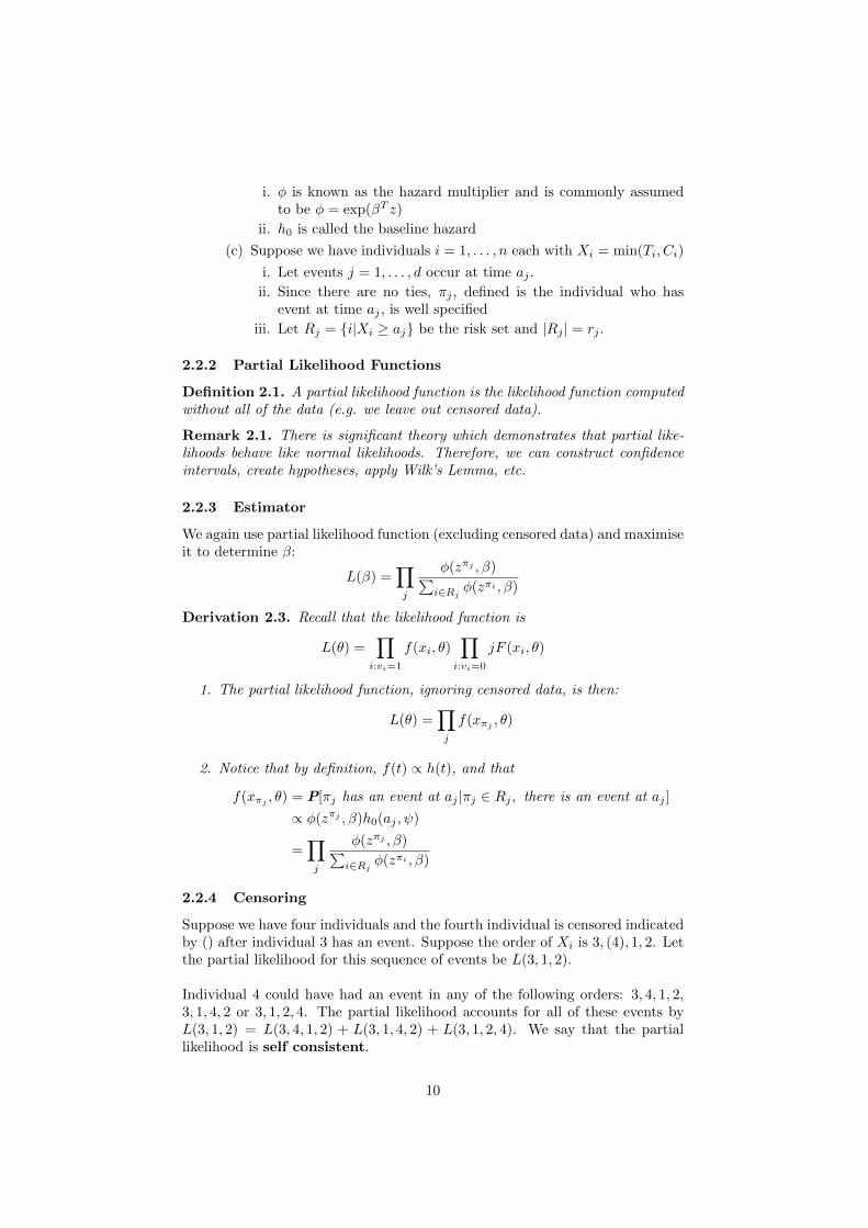
i. φ is known as the hazard multiplier and is commonly assumedto be φ = exp(βT z)

ii. h0 is called the baseline hazard

(c) Suppose we have individuals i = 1, . . . , n each with Xi = min(Ti, Ci)

i. Let events j = 1, . . . , d occur at time aj .

ii. Since there are no ties, πj , defined is the individual who hasevent at time aj , is well specified

iii. Let Rj = {i|Xi ≥ aj} be the risk set and |Rj | = rj .

2.2.2 Partial Likelihood Functions

Definition 2.1. A partial likelihood function is the likelihood function computedwithout all of the data (e.g. we leave out censored data).

Remark 2.1. There is significant theory which demonstrates that partial like-lihoods behave like normal likelihoods. Therefore, we can construct confidenceintervals, create hypotheses, apply Wilk’s Lemma, etc.

2.2.3 Estimator

We again use partial likelihood function (excluding censored data) and maximiseit to determine β:

L(β) =∏j

φ(zπj , β)∑i∈Rj

φ(zπi , β)

Derivation 2.3. Recall that the likelihood function is

L(θ) =∏i:vi=1

f(xi, θ)∏i:vi=0

jF (xi, θ)

1. The partial likelihood function, ignoring censored data, is then:

L(θ) =∏j

f(xπj , θ)

2. Notice that by definition, f(t) ∝ h(t), and that

f(xπj, θ) = P[πj has an event at aj |πj ∈ Rj , there is an event at aj ]

∝ φ(zπj , β)h0(aj , ψ)

=∏j

φ(zπj , β)∑i∈Rj

φ(zπi , β)

2.2.4 Censoring

Suppose we have four individuals and the fourth individual is censored indicatedby () after individual 3 has an event. Suppose the order of Xi is 3, (4), 1, 2. Letthe partial likelihood for this sequence of events be L(3, 1, 2).

Individual 4 could have had an event in any of the following orders: 3, 4, 1, 2,3, 1, 4, 2 or 3, 1, 2, 4. The partial likelihood accounts for all of these events byL(3, 1, 2) = L(3, 4, 1, 2) + L(3, 1, 4, 2) + L(3, 1, 2, 4). We say that the partiallikelihood is self consistent.

10

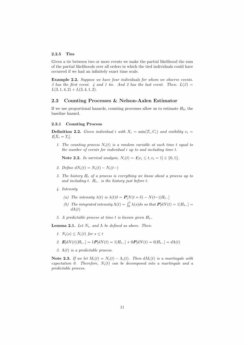
2.2.5 Ties

Given a tie between two or more events we make the partial likelihood the sumof the partial likelihoods over all orders in which the tied individuals could haveoccurred if we had an infinitely exact time scale.

Example 2.2. Suppose we have four individuals for whom we observe events.3 has the first event. 4 and 1 tie. And 2 has the last event. Then: L(β) =L(3, 1, 4, 2) + L(3, 4, 1, 2).

2.3 Counting Processes & Nelson-Aalen Estimator

If we use proportional hazards, counting processes allow us to estimate H0, thebaseline hazard.

2.3.1 Counting Process

Definition 2.2. Given individual i with Xi = min(Ti, Ci) and visibility vi =1[Xi = Ti].

1. The counting process Ni(t) is a random variable at each time t equal tothe number of events for individual i up to and including time t.

Note 2.2. In survival analysis, Ni(t) = 1[xi ≤ t, vi = 1] ∈ {0, 1}.

2. Define dNi(t) = Ni(t)−Ni(t−)

3. The history Ht of a process is everything we know about a process up toand including t. Ht− is the history just before t.

4. Intensity

(a) The intensity λ(t) is λ(t)δ = P[N(t+ δ)−N(t−)|Ht−]

(b) The integrated intensity Λ(t) =∫ t0λ(s)ds so that P[dN(t) = 1|Ht−] =

dΛ(t)

5. A predictable process at time t is known given Ht−

Lemma 2.1. Let Ni, and Λ be defined as above. Then:

1. Ni(s) ≤ Ni(t) for s ≤ t

2. E[dN(t)|Ht−] = 1P[dN(t) = 1|Ht−] + 0P[dN(t) = 0|Ht−] = dΛ(t)

3. Λ(t) is a predictable process.

Note 2.3. If we let Mi(t) = Ni(t) − Λi(t). Then dMi(t) is a martingale withexpectation 0. Therefore, Ni(t) can be decomposed into a martingale and apredictable process.

11

2.3.2 Counting Process in Survival Analysis

1. Intensity and Hazard: λ(t) is h(t) before an event happens, and is 0 afterit happens. Therefore, we can write dΛ = E[dNi(t)|Ht−] = Yi(t)hi(t).

(a) Yi(t) = 1[T ≥ t] is 1 before an event happens, and is predictable.

(b) Λi(t) =∫Yi(s)hi(s)ds =

∫Yi(s)dHi(s)

2. Notation

(a) N+(t) =∑iNi(t) is the data we have collected

(b) Λ+(t) =∑i

∫ t0

∫Yi(s)dHi(s) is what we want to estimate

(c) M+(t) = N+(t)− Λ+(t) is a mean zero martingale

2.3.3 General Estimator

1. Using the fact that M+(t) is a mean-zero martingale, our general estimatorwill use dN+(t) = dΛ+(t) + 0 to determine H0.

2. Assumption: hi(t) = φ(i)h0(t) and φ(i) are known

3. The general estimator is:

H0(t) =

∫ t

0

dN+(s)∑i Yi(s)φ(i)

Derivation 2.4. Using the fact that dN+(t) = dΛ+(t) =∑i Yi(t)φ(i)dH0(t),

we have:

dH0(t) =dN+(t)∑i Yi(t)φ(i)

H0(t) =

∫ t

0

dN+(s)∑i Yi(s)φ(i)

2.3.4 Nelson-Aalen Estmator

1. Assumptions: In addition to the assumptions for the general estimator,we assume that hj(t) are the same for all individuals, AND there are noties.

2. Let Y+(t) =∑i Yi(t). The Nelson-Aalen Estimator is then:

H0(t) =

∫ t

0

dN+(s)

Y+(s)=∑j:aj≤t

1

Y+(aj)

Derivation 2.5. By each assumption:

(a) If hi are all the same then hi(t) = h0(t). Therefore, H0(t) =∫ t0dN+(s)Y+(s)

(b) Suppose events happen at times a1, . . . , ag with no ties. Then dN+(s) =1[s = aj ] for j = 1, . . . , g. Moreover, Y+(aj) = rj the size of the risk

set at time aj. Therefore,∫ t0dN+(s)Y+(s) =

∑j:aj≤t

1Y+(aj)

12

3. Properties

(a) It is easily generalised when individuals enter or leave the risk set

(b) It is consistent with the Kaplan-Meier estimate for large n

(c) Censoring is handled by Y+

(d) Calculations of the estimator of the variance of the estimator arestraightforward

4. Dealing with Ties: Suppose we have a tie at aj

(a) One approach is to generalise the restrictions on dN+(t) and allowH0 = · · ·+ 1

rj−1+ 2

rj+ 1

rj+1+ · · ·

(b) A second approach assumes time is continuous: H0 = · · · + 1rj−1

+1rj

+ 1rj−1 + 1

rj+1+ · · ·

Remark 2.2. M(∞) = y′′ is the martingale residual used in model checking.

2.4 Log-Rank Test

2.4.1 Introduction

1. Purpose: Compares two survivor distributions with H0 : both groups areidentical

2. Notation

(a) Groups are denoted by i ∈ {0, 1}

(b) Survivor function at time t = aj in group i is denoted F (i)(aj) = F(i)j

(c) Data: At time aj , r(i)j is the number at risk in group i and d

(i)j is the

number of events in group i. Let dj = d(0)j +d

(1)j and rj = r

(0)j + r

(1)j .

3. Contingency Table at time aj

Group 0 Group 1 Total

Event d(0)j d

(1)j dj

No Event r(0)j − d

(0)j r

(1)j − d

(1)j rj − dj

Total r(0)j r

(1)j rj

4. Properties of Elements in the Contingency Table under H0

(a) E[d(0)j ] =

djrjr0j

(b) Cov[d(0)j ] =

r(0)j r

(1)j dj(rj−dj)r2j (rj−1)

(see Hypergeometric Distributions)

13

2.4.2 Test

1. Assumptions: We assume discrete event times {a0 < a1 < · · · < ag} andthe null hypothesis F 0

j = F 1j for j = 1, . . . , g.

2. Testing Parameters:

(a) Statistic:: z = observed − expected =∑gj=1 d

(0)j −

∑gj=1

djrjr(0)j

(b) Variance of Statistic: s2 =∑gj=1

r(0)j r

(1)j dj(rj−dj)r2j (rj−1)

(c) Test Statistic: zs ∼ N(0, 1). We assume normality since we do not

know its distribution.

Derivation 2.6. For the statistic: zj = d0j −djrjr0j . We simply sum

over all values of j.

For the deviaiton:

Cov[z] =∑j

Cov[zj ] =∑j

Cov[d0j ] =∑j

r(0)j r

(1)j dj(rj − dj)r2j (rj − 1)

3. Power:

(a) The log-rank test works well if the survivor functions are in the sameproportional hazards family

(b) The log-rank test works poorly if the survivor functions have an in-tersection

4. Variants of the Log-Rank Test:

(a) Some argue that the event times with larger risk sets should beweighted more

(b) z =∑gj=1 wjzj , where wj = (rj)

p usually with p = 0, 0.5, 1.0 usually.

2.4.3 Stratification

1. Purpose: suppose we are comparing two groups and want to control foranother categorical variable

2. Statistic:

(a) Create a contingency table for each level in the category, and computezj for each category

(b) Compute z by summing over all zj in all levels of categories.

3. Matched Pair Analysis: each stratification contains two individuals so thateach stratum contributes at most 1 deviation value to the statistic.

2.4.4 Relative Risk

The relative risk is a measure of how to groups are. In the log-rank context,the relative risk is:

RR =

∑obs1∑exp1

/

∑obs0∑exp0

14

2.5 Model Checking

2.5.1 General Model Checking and Survival Analysis

1. General model checking has the following process:

(a) Generate and Fit the model

(b) Analyse the residuals - most of the time these are naturally defined

Remark 2.3. In Survival Analysis, residuals do not have a naturaldefinition and there is often more than one possible choice.

2. Regression Model Checking

(a) Residuals are typically observed value less the model value

(b) Usually, the distribution of the residuals is exactly or approximatelyknown

2.5.2 Cox-Snell Residuals

Proposition 2.1. Suppose T is a continuous time-to-event with integrated haz-ard H. Let U = H(T ). Then U ∼ exp(1)

Proof.

P[U ≤ t] = P[H(T ) ≤ t] = P[T ≤ H−1(t)]

= 1− F (H−1t) = 1− exp(−H(H−1t))

= 1− exp(−t)

1. Fit the model with H(t), and compute the Cox-Snell Residuals yi = H(xi)

2. If H is close to H then yi should be exponentially distributed by theproposition.

3. Compute the Kaplan-Meier curve for yi and compare it to the expectedexp(1) distribution

4. Determining the importance of a categorical variable:

(a) Suppose the categorical variable has values A and B. Compute yAiusing subjects in category A and yBi for subjects in category B.

(b) Compute the KM curve for each group of residuals and compare themto the exp(1) distribution.

2.5.3 Cox-Snell Residuals and Censoring

Without censoring, E[yi] = 1, but when censoring occurs E[yi] < 1 becausexi < Ti, so it will pull the Kaplan-Meier curve for yi down and to the left of theexp(1) curve. There are two ways we can fix this:

Note 2.4. E[vi] = 1P[Xi ≥ Ti] ∼ H(xi).

15

1. Modified Cox-Snell: y′i = (1 − vi) + H(xi). This accounts for censoringsince with or without censoring, E[y′i] = 1.

2. Martingale Residuals: y′′i = vi − H(xi). This is similar to the “observed-expected” residual, and E[y′′i ] = 0.

2.5.4 Martingale Residuals

1. Fit the model, excluding a (continuous) explanatory variable z, and cal-culate y′′i

2. Plot y′′i against the values of zi.

(a) If the model, which excludes z, is sufficient, y′′i should form an ap-proximately horizontal line

(b) If the model is incorrect, we should use nonparametric methods tocompute y′′ = g(z) and include g(z) in the model.

Example 2.3. If we use the cox model, and assume φ(β, ζ) = exp(βT ζ),we can test whether a variable z should be used in this model. If wesee that it should, we have φ(β, ζ, z) = exp(βT [ζ g(z)])

3. Compute y′′i using the new model and ensure that the line is horizontal.

3 Advanced/Assorted Topics

3.1 Relative Survival Modelling (Estimation)

3.1.1 Introduction & Motivation

1. Motivation: Suppose we are observing two groups undergoing the sametreatment, but have naturally different hazards. To account for this, wesplit h(t) = hB(t) + hE(t).

(a) hB is the background hazard and refers to the hazard an individualhas based on their circumstances, and it is usually known (govern-ments usually publish this information)

(b) hE is the excess hazard, and is due to some factor that we are inter-ested in learning about, such as a treatment

2. Distributions and Interpretations

(a) We can compute the integrated background and excess hazardsHB , HE

and the background and excess survivor functions FB , FE .

(b) Background integrated hazard and survivor function have their nat-ural interpretation

(c) Excess integrate hazard and survivor function are fictitious functionswe would expect to see if the background were not present

Example 3.1. Suppose we treat a group of patients in Scotland and England,and see that survival is lower in Scotland than in England. By using relativesurvival modelling, we see that this is due to the fact that hScotlandB > hEnglandB

while hE is the same for both countries.

16

3.1.2 Parametric Likelihood Based Estimation

1. Assumptions

(a) We assume hiB(t) and HiB(t) are known

(b) We assume hiE(t) is the same for all subjections,and is hE(t)

(c) We assume we know the form (parametric) of hE(t, θ).

2. The function s based on the Likelihood which we maximise to estimate θand hence hE is:

s(θ) =∑i

vi log[hE(xi, θ) + hiB(xi)]−∑i

HE(xi, θ)

3. Maximisation to determine θ requires a numerical approach.

Derivation 3.1. Using the second assumption, the partial likelihood func-tions is:

s(θ) =∑i

vi log[hE(xi, θ) + hiB(xi)]−∑i

HE(xiθ) +HiB(xi)

=∑i

vi log[hE(xi, θ) + hiB(xi)]−∑i

HE(xiθ)

The second line follows from the fact that HiB(xi) are known constants

and will not play a role in the maximisation.

Example 3.2. Suppose we assume the form of hE(t) = θ and so HE(t) = tθ.Then:

s(θ) =∑i

vi log[θ + hiB ]− θ∑i

xi

Let X =∑i xi and d =

∑i vi. Taking the derivative we have:

s′(θ) =∑i

viθ + hiB

−X

With the added assumption that all hiB = h, we can set the derivative to 0 and

solve to get θ = dX − h. However, this is silly, but if we assume that hi � θ we

guess that we can have a similar solution:

θ =d

X− ε ≈ d

X− 1

d

∑i

vihiB

Derivation 3.2. We start by plugging in s′(θ) with θ = dX − ε

1. Plugging this in, rearranging, and setting it equal to 0, we have:

s′(θ) =∑i

vi

hiB + dX − ε

−X

=X

d

∑i

vi

1 + Xd (hiB − ε)

−X

d =∑i

vi

1 + Xd (hiB)− ε

17

2. Expanding the function as a Taylor series, and solving for ε we have:

d =∑i

vi(1−X

d(hiB)− ε)

d2 = d∑i

vi −X∑i

vihiB −Xε

∑i

vi

ε =1

d

∑i

vihiB

3.1.3 Nonparametric Counting Process Estimation

1. Note that HE(t) = H(t) − HB(t). By estimating H(t) as we do in thecounting process, we can estimate HE(t).

2. The estimator is:

HE(t) =

∫ t

0

dN+(u)

Y+(u)−∫ t

0

∑i Yi(u)hiB(u)du

Y+(u)

(a) The first term is the Nelson-Aalen Estimator

(b) The second term is the weighted average of the background hazardby all individuals who have not had an event as of time t (since Yi = 1if T > t)

Derivation 3.3. Using the counting process:

(a) Recall: dN+(t) = dΛ+(t) =∑i YidHE(t) +

∑i Yih

iB(t)

(b) Rearranging, we have: dHE(t) =dN+(t)−

∑i YIh

iB(t

Y+(t)

(c) We integrate to get the desired estimator

3. Beware that the first term is piecewise constant and the second is increas-ing, which may cause HE(t) < 0 over some intervals.

(a) We can fix this by: ignoring the relative parts, interpolating HE

between event times, or forcing HE to be piecewise constant betweenevent times.

(b) However, these fixes do not work if HE is negligible compared to HB ,or the disease preferentially affects a robust set.

3.2 Multiple Events Analysis: Marginal Modelling (Esti-mation)

3.2.1 Introduction

1. Multiple events analysis sutdies the case when more than one event ispossible per individual; hence, a correlation exists between events.

2. Types of Multiple Events:

18

(a) Sequential: a person has events that occur in sequence (e.g. a personhas headaches)

(b) Parallel: multiple time-to-events are being measured for the sameindividual (e.g. time until fillings in a subject’s mouth fall out)

3. Dealing with Correlations

4. Frailty: assuming there is a hidden/latent variable (called Frailty) whichcreates a random effect between the correlated events. By conditioningon frailty, the events are conditionally independent.

5. Marginal Modelling: we analyse the data, ignoring dependence, and thenwe adjust for this dependence by altering the variance.

3.2.2 Jack-Knife

1. Purpose: The Jack-Knife is a method for computing the variance of anestimator when traditional methods fail.

2. Methodology

(a) Let Ji = ˆbetai − β where ˆbetai is an estimate of β if we remove theith observation. Thus, Ji is essentially a measure of the influence ofthe ith data point on the estimator.

(b) ˆCov[β] = n−1n

∑i(Ji − J)(Ji − J)T is the variance estimator

3. Properties

(a) The Jack-knife is a robust, consistent and unbiased estimator whenthe data point left out is independent of the others

(b) Jack-knife estimator for variance of normally distributed data is theusual variance estimator

3.2.3 Estimators

1. We assume a proportional hazards model and want to estimate β

2. The Newton-Raphson Method

(a) Use the partial log-likelihood function to compute the score functionU(β) and information matrix I(β).

(b) Starting with some β(0), we iteratively compute

β(k+1) = β(k) + I−1(β(k))U(β(k))

(c) As k →∞, the iterated estimates converge to β

3. Computing the Variance of the Estimator

(a) We can compute the variance of the estimator using the Jack-knifemethod

19

(b) To compute βi, we can reiterate using the Newton-Raphson Method

starting with β but by removing the ith data point altogether whencomputing the partial likelihood, score and information matrix.

4. In multiple event analysis, we leave out the entire subset of data associatedwith the ith subject instead of just the ith data point, since the subjectsare independent.

3.2.4 Generic Data Structure

Example 3.3. Suppose we are observing individuals who are normal. Theseindividuals can either: progress into disease and then die, or die. Thereforethere are three possible strata that exist:

1. Living → disease progression

2. Living → death

3. Disease Progression → death

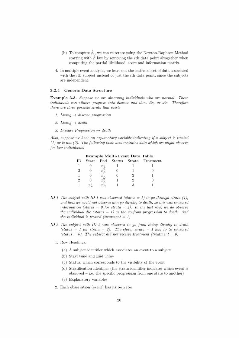
Also, suppose we have an explanatory variable indicating if a subject is treated(1) or is not (0). The following table demonstrates data which we might observefor two individuals:

Example Multi-Event Data TableID Start End Status Strata Treatment1 0 x1A 1 1 12 0 x2A 0 1 01 0 x1A 0 2 12 0 x2A 1 2 01 x1A x1B 1 3 1

ID 1 The subject with ID 1 was observed (status = 1) to go through strata (1),and thus we could not observe him go directly to death, so this was censoredinformation (status = 0 for strata = 2). In the last row, we do observethe individual die (status = 1) as the go from progression to death. Andthe individual is treated (treatment = 1)

ID 2 The subject with ID 2 was observed to go from living directly to death(status = 1 for strata = 2). Therefore, strata = 1 had to be censored(status = 0). The subject did not receive treatment (treatment = 0).

1. Row Headings:

(a) A subject identifier which associates an event to a subject

(b) Start time and End Time

(c) Status, which corresponds to the visibility of the event

(d) Stratification Identifier (the strata identifier indicates which event isobserved – i.e. the specific progression from one state to another)

(e) Explanatory variables

2. Each observation (event) has its own row

20

3.3 Frailty (Estimation)

3.3.1 Introduction

1. Motivation: often we are unable to include explanatory variables, espe-cially if they are unknown to us. Typically, the effect of these variablesare absorbed by the error term with randomisation. However, this doesnot always occur in survival analysis.

2. Problem Formulation:

(a) Each subject has an unknown frailty (unknown explanatory variable),which we typically believe is non-negative

(b) The higher an individual’s frailty, the higher the risk of an event

3. Notation:

(a) Let U ≥ 0 be the frailty random variable

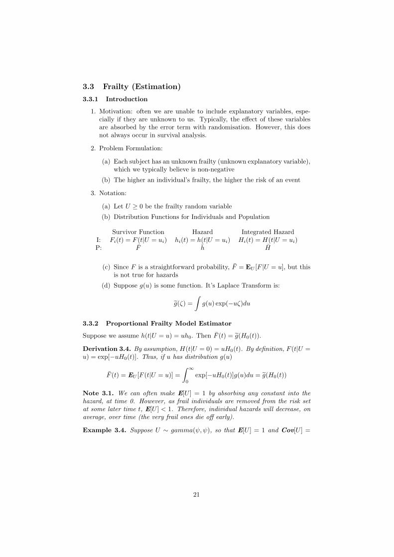
(b) Distribution Functions for Individuals and Population

Survivor Function Hazard Integrated HazardI: Fi(t) = F (t|U = ui) hi(t) = h(t|U = ui) Hi(t) = H(t|U = ui)P: F h H

(c) Since F is a straightforward probability, F = EU [F |U = u], but thisis not true for hazards

(d) Suppose g(u) is some function. It’s Laplace Transform is:

g(ζ) =

∫g(u) exp(−uζ)du

3.3.2 Proportional Frailty Model Estimator

Suppose we assume h(t|U = u) = uh0. Then F (t) = g(H0(t)).

Derivation 3.4. By assumption, H(t|U = 0) = uH0(t). By definition, F (t|U =u) = exp[−uH0(t)]. Thus, if u has distribution g(u)

F (t) = EU [F (t|U = u)] =

∫ ∞0

exp[−uH0(t)]g(u)du = g(H0(t))

Note 3.1. We can often make E[U ] = 1 by absorbing any constant into thehazard, at time 0. However, as frail individuals are removed from the risk setat some later time t, E[U ] < 1. Therefore, individual hazards will decrease, onaverage, over time (the very frail ones die off early).

Example 3.4. Suppose U ∼ gamma(ψ,ψ), so that E[U ] = 1 and Cov[U ] =

21

ψ−1. We have the following population distributions:

F (t) =

(1

1 + H0(t)ψ

)ψ

h(t) =−F ′(t)F (t)

=h0(t)

1 + H0(t)ψ

h(t)

h0(t)=

(1 +

H0(t)

ψ

)−1

1. At t = 0, H0(t) =∫ 0

0h(s)ds = 0. So we have that the third equation is 1,

a consequence of E[U ] = 1.

2. As t > 0, the third equation will decreases since H0(t) is an increasingfunction. This correlates to E[U ] < 1 as time increases.

3. If ψ is small, Cov[U ] = ψ−1 is going to be large. So the third equationwill decrease rapidly as there will be individuals with very high frailtieswho will die very quickly.

3.3.3 Influence of Unknown Variables in Proportional Hazards Model

1. The influence of Unknown Variables:

(a) Suppose we have a simple treatment explanatory variable z ∈ {0, 1}and we model the ith individual in group z using proportional hazards

and proportional frailty: hi(t) = u(z)i eβzh0(t)

(b) Assume U ∼ gamma(ψ,ψ) and u(z)i are i.i.d. Then:

h(z)(t) =eβzh0(t)

1 + eβzH0(t)ψ−1

h(1)(t)

h(0)(t)= eβ

1 +H0(t)ψ−1

1 + eβH0(t)ψ−1

(c) Notice that although individual hazard ratios are proportional overtime, the population ratios change over time. So when we leave outan explanatory variable in proportional hazards, we do not capturethe early behaviour of the population.

2. Coping with Unknown Variables

(a) measure as many explanatory variables as possible and hope nothingis left out

(b) Move away from proportional hazards completely, and use a modelin which frailty will occur in the error (e.g. accelerated time family)

22

3.3.4 Inference of Frailty Variable

1. In general, F (t) = g(H0(t)). The RHS of the equality can take on manyforms of g and H0(t) and still achieve the same F (t) making inferencedifficult.

2. Moreover, we usually only have one observation (the event) for inference,making it nearly impossible to infer g

3. In multiple events, we can do better since we have multiple events per sub-ject. However, with too few events per individual, convergence is difficultto achieve.

3.4 Cure (Estimation)

3.4.1 Introduction

1. Motivation

(a) The cure model is a special case of frailty, in which some (unknown)fraction of the population is no longer at risk

(b) Typically, a cure model’s survivor function has levelled off, but thislevelling off can have multiple explanations, such as:

i. All subjects have very low risk

ii. Some subjects have high risk, and some have a low risk

(c) Therefore, choosing a cure model requires scientific input and evi-dence

2. Notation

(a) The probability and individual is cured is πi = π(β, yi), where yare explanatory variables and β are parameters, and π is a functiontaking values in [0, 1].

(b) The at risk/diseased fraction has distributions subscripted by a D:hD, fD, HD, FD. We do not observe these values

(c) We do observe hT , fT , HT , FT for the whole population, where theseparameters depend on parameters (γ) and explanatory variables (zi).

3. Typical Parametrisation

(a) πi =(1 + exp[−βT yi]

)−1for an unknown β

(b) F iD = exp[−(exp(−γT zi)t

)k](Weibull) for unknown γ and k (k is

an index in this context).

(c) HiD =

(exp(−γT zi)t

)k

23

3.4.2 Simple Model

1. The Simple Model

(a) F iT (t) = πi + (1− πi)F iD(t)

(b) f iT (t) = (1− πi)f iD(t) is an improper distribution

(c) s(γ, β, k) =∑i log[(1−πi)f iD(t)] +

∑i(1− vi) log[πi + (1−πi)F iD(t)]

2. Practical considerations when maximising s to determine γ, β, k

(a) y and z may have common elements, so check Cov[y, z] to see whatparameters may interfere.

(b) We need to have many follow ups to ensure that an individual whois censored is actually cured.

3.4.3 Extensions to Simple Model

The first extension uses background mortality (hazard) to better model FT . Thesecond extension considers a semi-parametric proportional hazards modelling tobetter model FT .

1. Adding Background Mortality

(a) Let the vulnerable fraction have a background and excess hazard(HD(t) = HB(t) +HE(t)).

(b) Let the cured fraction have only a background hazard (HB(t))

(c) Then, FT (t) = πFB(t) + (1− π)FB(t)FE(t).

(d) Compute fT and the log-likelihood s accordingly and maximise todetermine the unknown parameters.

2. Adding Proportional Hazards Modelling

(a) Model: hD(t) = exp[γT z]h0(t)

(b) We then compute the distributions and log-likelihood:

i. F iD(t) = exp(−eγT zH0(t)

)ii. f iD(t) =

(eγ

T zh0(t))

exp(−eγT zH0(t)

)iii. s =

∑i vi log[(1− πi)

(eγ

T zih0(t))

exp(−eγT ziH0(t)

)]

+∑i(1− vi) log[πi − (1− πi) exp

(−eγT ziH0(t)

)]

Note 3.2. We can write exp(−eγT zH0(t)

)= [F0(t)]

exp(γT z)

(c) Because the baseline hazards do not cancel (since the hazard is onlyproportional to in hD not hT ), h0 and F0 are nonparametric portionswhich cannot be directly maximised

(d) In this situation, we use expectation maximisation to determine es-timates for β and γ

24

3.4.4 Expectation Maximisation

Suppose we knew qi = 1[individual i is vulnerable], then we could model thecured and diseased groups separately allowing us to determine β and γ. Wewould have the following log-likelihood for β and partial likelihood (based onproportional hazards models) for γ:

s1(β) =∑i

(1− qi) log[πi(β, yi)] + qi log[πi(β, yi)]

L2(γ) =∏

j:qj=1

eγT zj∑

i∈RjeγT zi

Note that we purposefully excluded the πj notation for proportional hazards toavoid confusion, but this should be computed using the πj notation. In expec-tation maximisation, we make an initial guess for qi, compute the parameters,then update qi until we have convergence. Algorithm:

1. Guess qi = vi

2. Estimate β using the log-likelihood s1

3. Estimate γ using the partial-likelihood L2

4. Estimate F0 and h0 as well (Nelson-Aalen)

5. Updated qi = P[i is at risk|i is censored at xi] = F (xi)(1−πi)

πi+F (xi)(1−πi)

6. Repeat the steps using the new qi until qi converges

3.5 Empirical Likelihood

3.5.1 Introduction

1. Objective: We want to use nonparametric methods (empirical likelihood)to derive the survivor function and obtain point and interval estimates fortime-to-event probabilities

2. Properties: the empirical likelihood function must satisfy the conditionsof the survivor function F (t):

(a) Non-increasing

(b) Non-negative

(c) Bounded above by 1

3. Constructing the empirical likelihood from data:

(a) Individual contributions to the likelihood:

i. If vi = 1, then P[T = xi] = F (xi)− F (xi−)

ii. If vi = 0, and T > xi (right censored), then P[T > xi] = F (xi)

iii. If vi = 0, and T ≤ xi (left censored), then P[T ≤ xi] = 1−F (xi)

25

iv. If vi = 0, and T ∈ [xLi , xUi ] (interval censored), then P[T ∈

[xLi , xUi ]] = F (xLi )− F (xUi )

(b) Common simplifications

i. We assume we only have events or right censoring

ii. If vi = 1 then F (xi−) =

F (the largest preceding time when an event occured)

iii. If vi = 0 then F (xi) =

F (the largest preceding time when an event occured)

3.5.2 Derivation of Kaplan-Meier

1. Assuming the simplifications, and:

(a) Suppose a1 < a2 < · · · < ag are event times, and let a0 = 0, ag+1 =∞

(b) Suppose dj ≥ 1 events occur at the event times with subscript j =1, . . . , g.

(c) Suppose cj individuals are censored between [aj , aj+1]

2. The likelihood functions are then:

(a) The likelihood function:

L =

g∏j=1

[P[T = aj ]]dj [P[T > aj ]]

cj

=

g∏j=1

[F (aj−1)− F (aj)]dj [F (aj)]

cj

(b) The log-likelihood function:

s =

g∑j=1

dj log[F (aj−1)− F (aj)] + cj log[F (aj)]

(c) The partial derivative of the log-likelihood:

∂s

∂F (aj)=

djF (aj)− F (aj+1)

+cj

F (aj)− djF (aj−1)− F (aj)

3. We have the Kaplan-Meier by the following procedure:

(a) Set the partial derivative to 0 for event time ag and solve to get:

F (ag) =cg

cg+dgF (ag−1)

(b) Let rg = cg + dg and rj = rj+1 + cj + dj giving: F (ag) = (1 −dgrg

)F (ag−1)

(c) Prove by induction: F (0) = 1, then

F (aj) =

(1− dg

rg

)F (aj−1)

26

3.5.3 Constrained Maximisation for Interval Estimation

Note 3.3. We can generate an interval for each F(t) by creating a profile curveF (t) = z ∈ [0, 1]. This is the same as before, but here we describe the method ofdoing it.

Method of Lagrangian Multipliers.

1. Suppose we have the constraint that Fk = z

2. Let the Lagrangian S(λ) =∑gj=1 dg log[Fj−1−Fj ]+cj log[Fj ]+λ(log[Fk]−

log[z])

3. We want to maximise S with respect to all λ which also satisfies theconstraint.

4. Using the recurrence relationship used to derive the KM Estimator, wenote:

(a) Starting with Fk = z, Fj = (1− djrj

)Fj−1 for j > k

(b) Starting with F0 = 1, we need to find the λ which satisfies Fk = 0

using the recurrence Fj = (1− djrj

+ λ)Fj−1 for j ≤ k

Remark 3.1. In practice, it is easier to simply start with values of λ andcompute the z to which they correspond.

3.6 Schoenfeld Residuals (Model Checking)

3.6.1 Introduction

1. In the Cox Model, we want to estimate β where hi(t) = h0(t) exp[βT z].Cox-Snell and Martingale residuals allowed us to evaluate the plausibilityof βT z relationship and replace it with βT g(z) if necessary. Schoenfeldresiduals allow us to determine the time dependence of β.

2. Notation

(a) Let Yi(t) = 1[i ∈ Rt](b) Let wi(t) = Yi(t) exp[βT zi]

(c) Let zj(β) =∑

i wizi∑i wi

be the weighted average of the explanatory vari-

ables in the risk set at time aj

3. Assumptions

(a) We assume the Cox (Proportional Hazards) Model

(b) We assume there are no ties and d events occurring at time a1 <a2 < · · · < ad

27

4. Recall from the Cox Model that the likelihood, log-likelihood, score andinformation are:

L(β) =∏j

exp[βT zπj ]∑i wi(aj)

s(β) =∑j

βT zπj − log[∑i

wi(aj)]

U(β) =∑j

zπj −∑i ∂βwi(aj)∑i wi(aj)

=∑j

zπj − zj(β)

I(β) = −∂βU(β) =∑j

∂β zj(β)

3.6.2 Schoenfeld Residual and Applications

The Schoenfeld residual is defined based on the score function, by noting thatif β does not have a time dependence U(β) = 0.

Definition 3.1. Let the Schoenfeld Residual be sj(β) = zπj−zj(β). Let s∗j (β) =

I−1(β)sj(β)

Lemma 3.1. Therefore, U(β) =∑j sj(β) and E[s∗j (β)] = θg(aj)

Proof. The first equality follows from the definitions of U and sj . To prove thesecond equality (with hand-waving):

1. Let β(t) = β0+θg(t). Notice that adding or subtracting a constant to g(t)will get absorbed in proportional hazards modelling by the exponentialterm. So we can scale the function to ensure that E[β] = β0

2. Given that the correct form of the parameter is β(t), we have that:

(a) E[sj(β0)] = zj(β(aj))− zj(β0) = zj(β0 + θg(aj))− zj(β0)

(b) By Taylor Expansion:

E[sj(β0)] = zj(β0+θg(aj))−zj(β0) =∑j

∂β zj |β0θg(aj) = I(β0)θg(aj)

(c) Therefore, E[s∗j (β0)] = E[I−1sj(β0)(β0)] = θg(aj)

3. Using β as an estimator for β0, we have the desired property.

Application: We can compute s∗j (β) and plot it against aj .

1. If β does not have a time-dependence, then the line will be horizontal

2. IF β hat does have a time-dependence, we can compute θg(t) using non-parametric methods.

28

3.7 Planning Experiments: Determining size of a Study

3.7.1 Introduction

1. Objective: To determine how many subjects we need in a study to con-clude that one treatment is better than another, given a significant levelα and power 1− β

2. Assumptions

(A0) The test statistic, U , is normally distributed under the null and al-ternative hypotheses

(A1) We assume the hazards under the two treatments (0,1) are propor-tional

(A2) There are no ties in the data

(A3) Risk sets between both treatments remain equal at all times

(A4) We assume survivor functions under both treatments are exponential

3. Revision of Testing Treatments

(a) Hypothesis: we are hoping and expecting µ1 > µ2, else we would notdo this test. By (A0):

H0: U ∼ N(µ0, σ20)

H1: U ∼ N(µ1, σ21)

(b) Test Characteristics

i. P[rejecting H0|H0 is true] = α called the significance

ii. P[rejecting H0|H1 is true] = 1− β called the power

4. Under the Log Rank Test with U = zs , by assumption (A0)

H0: U ∼ N(0, 1)

H1: U ∼ N(µ1, σ21), but the parameters are unknown

5. Notation: Let d =∑j 1

3.7.2 Sample Size Inequality

We first note that to achieve a significance level of α under H0, we have forsome critical value C:

α/2 = P[U > C|H0]

= P[U − µ0

σ0>C − µ0

σ0|H0]

= 1− Φ

(C − µ0

σ0

)C = σ0Φ−1(1− α/2) + µ0

29

Noting that we expect µ1 > µ2, to achieve the power level 1− β under H1, wehave for the same critical value C:

1− β ≤ P[U > C|H1]

≤ P[U − µ1

σ1>C − µ1

σ1|H1]

≤ 1− Φ

(C − µ1

σ1

)C ≤ σ1Φ−1(β) + µ1

Combining the two results, we have the sample size inequality:

µ1 − µ0 ≥ σ0Φ−1(1− α/2)− σ1Φ−1(β) or

µ1 − µ0 ≥ σ0Φ−1(1− α/2) + σ1Φ−1(1− β)

3.7.3 Parameters under H0

We want to compute the form, expectation and variance of U under H0. Underassumptions (A2) and (A3) we that dj = 1 and r0j = r1j . Under H0, we havethat:

1. E[d0j ] = P[d0j = 1|H0] = 0.5. Under H0 there is no difference between thetreatments, so either an event occurs under treatment 1 or treatment 0,and both should have the same probability.

2. Cov[d0j ] = E[(d0j )2]−(E[d0j ])

2 = 12P[d0j = 1|H0]−0.25 = 0.5−0.25 = 0.25

3. U =(∑

j d0j )−d/2√d/4

4. E[U ] = 0 = µ1 as desired

5. Cov[U ] = 1 = σ20 as desired

Derivation 3.5. Recall from the Log-Rank test that the form of U =∑

j obs−exp√Cov[

∑j obs−exp]

.

Therefore:

1. U =∑

j d0j−1/2√∑

j Cov[d0j ]which is what we are looking for

2. E[U ] = 2√d(∑j(E[d0j ])− d/2) = 0

3. Cov[U ] = 4d

∑j Cov[d0j ] = 1

3.7.4 Parameters under H1

We want to compute the form, expectation and variance of U under H1. Underassumption (A1), h0(t)/h1(t) = λ. Under H0, λ = 1, and under H1, λ > 1.Under H1 we have that:

1. P[d0j = 1|H1] = λ1+λ

2. E[d0j ] = λ1+λ and Cov[d0j ] = λ

(1+λ)2

30

3. E[U ] =√dλ−1λ+1 and Cov[U ] = 4λ

(1+λ)2

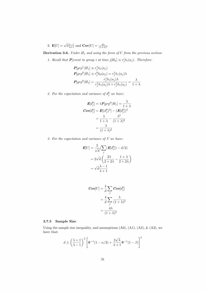
Derivation 3.6. Under H1 and using the form of U from the previous section:

1. Recall that P[event in group i at time j|Hk] ∝ rijhi(aj). Therefore:

P[grp1|H1] ∝ r1jh1(aj)

P[grp0|H1] ∝ r0jh0(aj) = r1jh1(aj)λ

P[grp0|H1] =r1jh1(aj)λ

r1jh1(aj)λ+ r1jh1(aj)=

λ

1 + λ

2. For the expectation and variance of d0j we have:

E[d0j ] = 1P[grp0|H1] =λ

1 + λ

Cov[d0j ] = E[(d0j )2]− (E[d0j ])

2

=λ

1 + λ− λ2

(1 + λ)2

=λ

(1 + λ)2

3. For the expectation and variance of U we have:

E[U ] =2√d

(∑j

(E[d0j ])− d/2)

= 2√d

(2λ

2 + 2λ− 1 + λ

2 + 2λ

)=√dλ− 1

λ+ 1

Cov[U ] =4

d

∑j

Cov[d0j ]

=4

d

∑j

λ

(1 + λ)2

=4λ

(1 + λ)2

3.7.5 Sample Size

Using the sample size inequality, and assumptions (A0), (A1), (A2), & (A3), wehave that:

d ≥(λ+ 1

λ− 1

)2[

Φ−1(1− α/2) +2√λ

λ+ 1Φ−1(1− β)

]2

31

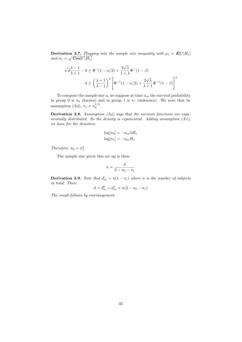
Derivation 3.7. Plugging into the sample size inequality with µ1 = E[U |H1]and σ1 =

√Cov[U |H1]

√dλ− 1

λ+ 1− 0 ≥ Φ−(1− α/2) +

2√λ

1 + λΦ−(1− β)

d ≥(λ+ 1

λ− 1

)2[

Φ−1(1− α/2) +2√λ

λ+ 1Φ−1(1− β)

]2To compute the sample size n, we suppose at time am the survival probability

in group 0 is π0 (known) and in group 1 is π1 (unknown). We note that by

assumption (A4), π1 = π1/λ0 .

Derivation 3.8. Assumption (A4) says that the survivor functions are expo-nentially distributed. So the density is exponential. Adding assumption (A1),we have for the densities:

log[π0] = −amλH1

log[π1] = −amH1

Therefore, π0 = πλ1 .

The sample size given this set up is then:

n =d

2− π0 − π1

Derivation 3.9. Note that dim = n(1 − πi) where n is the number of subjectsin total. Then:

d = d0m + d1m = n(2− π0 − π1)

The result follows by rearrangement.

A Likelihood Tests and Properties

32

Hypothesis Tests and Con�dence Regions Usingthe Likelihood

F. P. Treasure

13-May-053020a

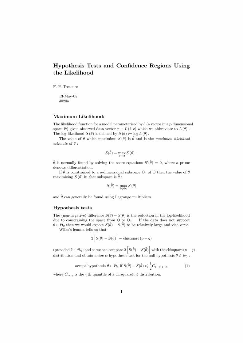
Maximum Likelihood:

The likelihood function for a model parameterised by � (a vector in a p-dimensionalspace �) given observed data vector x is L (�jx) which we abbreviate to L (�) .The log-likelihood S (�) is de�ned by S (�) := logL (�) :The value of � which maximizes S (�) is � and is the maximum likelihood

estimate of � :

S(�) = max�2�

S (�) .

� is normally found by solving the score equations S0(�) = 0, where a primedenotes di¤erentiation.If � is constrained to a q-dimensional subspace �0 of � then the value of �

maximizing S (�) in that subspace is ~� :

S(~�) = max�2�0

S (�)

and ~� can generally be found using Lagrange multipliers.

Hypothesis tests

The (non-negative) di¤erence S(�)� S(~�) is the reduction in the log-likelihooddue to constraining the space from � to �0 . If the data does not support� 2 �0 then we would expect S(�)� S(~�) to be relatively large and vice-versa.Wilks�s lemma tells us that:

2hS(�)� S(~�)

i� chisquare (p� q)

(provided � 2 �0) and so we can compare 2hS(�)� S(~�)

iwith the chisquare (p� q)

distribution and obtain a size � hypothesis test for the null hypothesis � 2 �0 :

accept hypothesis � 2 �o if S(�)� S(~�) 61

2Cp�q;1�� (1)

where Cm; is the th quantile of a chisquare(m) distribution.

1

Con�dence Regions and Intervals

A p-dimensional 1�� con�dence region can be constructed by letting �0 consistof the single point �0 and including �0 in the con�dence region if the hypothesistest � 2 �0 �equivalently: � = �0 �is not rejected by rule (1). The con�denceregion is therefore (noting here that q = 0 and ~� = �0 ):�

�0 : S(�)� S (�0) 61

2Cp�q;1��

�.

A con�dence interval is a one-dimensional con�dence region and is obtainedwhen either � is one-dimensional (p = 1) or we are interested in a single com-ponent of � . In the latter case we partition � as � = [� ]T where � is a scalar(parameter of interest) and is (p� 1)-dimensional (the nuisance parameters).The maximum likelihood estimate � is now [� ]T. The symbols and canbe ignored if � is one-dimensional.The con�dence interval will be of form L 6 �0 6 U and is given by:�

�0 : S(�; )� S(�0; ~ ) 61

2C1;1��

�where ~ is de�ned by S(�0; ~ ) = max[� ]T2�;�=�0 S (�; ) .

Other Tests Based on the Likelihood

The above tests and con�dence regions are based on the di¤erence in log-likelihoods and are referred to as likelihood-ratio tests etc. They are (in myview) the best ones to use. For historical and computational reasons twoother approaches are commonly seen. They are based on approximating thelog-likelihood function by a quadratic and are both asymptotically equivalentto likelihood-ratio methods. The tests are in practice only as good as thequadratic approximation (usually good enough)I shall present the approximate methods using the simplest case: a hypoth-

esis test for a single scalar parameter (that is: p = 1 and q = 0). In theoreticalwork the expectation ES00 (�) is often used instead of the observed S00 (�) : thisis rarely practicable (and arguably not desirable) in survival analysis.

The Wald Test

The log-likelihood is approximated by a quadratic at � = � . The statistic fortesting the null hypothesis that � = �0 is

��� � �0

�2S00(�)

which is compared with the chisquare(1) distribution. Many computer pro-grams report the reciprocal of the square root of S00(�) as the estimated stan-dard deviation of � (the �standard error�).

2

The Score Test

The log-likelihood is approximated by a quadratic at � = �0 . This has the hugecomputational advantage that the log-likelihood does not have to be maximized.The test statistic is:

[S0 (�0)]2

�S00 (�0), (2)

again, compared with the chisquare(1) distribution.Exercise (hard(ish)): show that the score test applied to a proportional

hazards model of a two group comparison gives the log-rank test. Hint: ignorethe denominator in both (2) and the log-rank statistic as they merely normalisethe variance to unity �concentrate on showing the numerators are proportional.

References

1. Therneau T. M. and Grambsch P. M. (2000) Modelling Survival Data �Extending the Cox Model. Springer-Verlag [see chapter three for use-ful summary and examples and an illustration of what to do when thequadratic approximation breaks down]

2. Wilks S. S. (1938) The large-sample distribution of the likelihood ratio fortesting composite hypotheses. Annals of Mathematical Statistics 9:60-62

3