Notes for Math 261A Lie groups and Lie algebras
179
Notes for Math 261A Lie groups and Lie algebras June 28, 2006 Contents Contents . . . . . . . . . . . . . . . . . . . . . . . . . 1 How these notes came to be . . . . . . . . . . . . . . . . . 3 Lecture 1 . . . . . . . . . . . . . . . . . . . . . . . . 4 Lecture 2 . . . . . . . . . . . . . . . . . . . . . . . . 6 Tangent Lie algebras to Lie groups,6 Lecture 3 . . . . . . . . . . . . . . . . . . . . . . . . 9 Lecture 4 . . . . . . . . . . . . . . . . . . . . . . . . 12 Lecture 5 . . . . . . . . . . . . . . . . . . . . . . . . 16 Simply Connected Lie Groups, 16 Lecture 6 - Hopf Algebras . . . . . . . . . . . . . . . . . . 21 The universal enveloping algebra, 24 Lecture 7 . . . . . . . . . . . . . . . . . . . . . . . . 26 Universality of U g, 26 Gradation in U g, 27 Filtered spaces and algebras, 28 Lecture 8 - PBW theorem, Deformations of Associative Algebras . . 31 Deformations of associative algebras, 32 Formal deformations of associative algebras, 34 Formal deformations of Lie algebras, 35 Lecture 9 . . . . . . . . . . . . . . . . . . . . . . . . 36 Lie algebra cohomology, 37 Lecture 10 . . . . . . . . . . . . . . . . . . . . . . . . 41 Lie algebra cohomology, 41 H 2 (g, g) and Deformations of Lie algebras, 42 Lecture 11 - Engel’s Theorem and Lie’s Theorem . . . . . . . . . 46 The radical, 51 Lecture 12 - Cartan Criterion, Whitehead and Weyl Theorems . . . 52 Invariant forms and the Killing form, 52 Lecture 13 - The root system of a semi-simple Lie algebra . . . . . 59 Irreducible finite dimensional representations of sl(2), 63 Lecture 14 - More on Root Systems . . . . . . . . . . . . . . 65 Abstract Root systems, 66 The Weyl group, 68 Lecture 15 - Dynkin diagrams, Classification of root systems . . . . 71 Isomorphisms of small dimension, 76 1
Transcript of Notes for Math 261A Lie groups and Lie algebras

Notes for Math 261A
Lie groups and Lie algebras
June 28, 2006
Contents
Contents . . . . . . . . . . . . . . . . . . . . . . . . . 1How these notes came to be . . . . . . . . . . . . . . . . . 3Lecture 1 . . . . . . . . . . . . . . . . . . . . . . . . 4Lecture 2 . . . . . . . . . . . . . . . . . . . . . . . . 6
Tangent Lie algebras to Lie groups, 6
Lecture 3 . . . . . . . . . . . . . . . . . . . . . . . . 9Lecture 4 . . . . . . . . . . . . . . . . . . . . . . . . 12Lecture 5 . . . . . . . . . . . . . . . . . . . . . . . . 16
Simply Connected Lie Groups, 16
Lecture 6 - Hopf Algebras . . . . . . . . . . . . . . . . . . 21The universal enveloping algebra, 24
Lecture 7 . . . . . . . . . . . . . . . . . . . . . . . . 26Universality of Ug, 26Gradation in Ug, 27Filtered spaces and algebras, 28
Lecture 8 - PBW theorem, Deformations of Associative Algebras . . 31Deformations of associative algebras, 32Formal deformations of associative algebras, 34Formal deformations of Lie algebras, 35
Lecture 9 . . . . . . . . . . . . . . . . . . . . . . . . 36Lie algebra cohomology, 37
Lecture 10 . . . . . . . . . . . . . . . . . . . . . . . . 41Lie algebra cohomology, 41H2(g, g) and Deformations of Lie algebras, 42
Lecture 11 - Engel’s Theorem and Lie’s Theorem. . . . . . . . . 46The radical, 51
Lecture 12 - Cartan Criterion, Whitehead and Weyl Theorems . . . 52Invariant forms and the Killing form, 52
Lecture 13 - The root system of a semi-simple Lie algebra . . . . . 59Irreducible finite dimensional representations of sl(2), 63
Lecture 14 - More on Root Systems . . . . . . . . . . . . . . 65Abstract Root systems, 66The Weyl group, 68
Lecture 15 - Dynkin diagrams, Classification of root systems . . . . 71Isomorphisms of small dimension, 76
1
2
Lecture 16 - Serre’s Theorem. . . . . . . . . . . . . . . . . 78Lecture 17 - Constructions of Exceptional simple Lie Algebras . . . 82Lecture 18 - Representations . . . . . . . . . . . . . . . . . 87
Representations, 87Highest weights, 89
Lecture 19 - The Weyl character formula . . . . . . . . . . . . 93The character formula, 94
Lecture 20 . . . . . . . . . . . . . . . . . . . . . . . . 100Compact Groups, 102
Lecture 21 . . . . . . . . . . . . . . . . . . . . . . . . 105What does a general Lie group look like?, 105Comparison of Lie groups and Lie algebras, 107Finite groups and Lie groups, 108Algebraic groups (over R) and Lie groups, 109
Lecture 22 - Clifford algebras and Spin groups . . . . . . . . . . 111Clifford Algebras and Spin Groups, 112
Lecture 23 . . . . . . . . . . . . . . . . . . . . . . . . 117Clifford Groups, 118
Lecture 24 . . . . . . . . . . . . . . . . . . . . . . . . 123Spin representations of Spin and Pin groups, 123Triality, 126More about Orthogonal groups, 127
Lecture 25 - E8 . . . . . . . . . . . . . . . . . . . . . . 129Lecture 26 . . . . . . . . . . . . . . . . . . . . . . . . 134
Construction of E8, 136
Lecture 27 . . . . . . . . . . . . . . . . . . . . . . . . 140Construction of the Lie group of E8, 143Real forms, 144
Lecture 28 . . . . . . . . . . . . . . . . . . . . . . . . 146Working with simple Lie groups, 148Every possible simple Lie group, 150
Lecture 29 . . . . . . . . . . . . . . . . . . . . . . . . 152Lecture 30 - Irreducible unitary representations of SL2(R) . . . . . 159
Finite dimensional representations, 159The Casimir operator, 162
Lecture 31 - Unitary representations of SL2(R) . . . . . . . . . 165Background about infinite-dimensional representations, 165The group SL2(R), 166
Solutions to (some) Exercises. . . . . . . . . . . . . . . . . 171References . . . . . . . . . . . . . . . . . . . . . . . . 176Index . . . . . . . . . . . . . . . . . . . . . . . . . . 178

3
How these notes came to be
Among the Berkeley professors, there was once Alan Knutson, who wouldteach Math 261. But it happened that professor Knutson was on sabbati-cal elsewhere (I don’t know where for sure), and eventually went there (orsomewhere else) for good. During this turbulent time, Maths 261AB werecancelled two years in a row. The last of these four semesters (Spring 2006),some graduate students gathered together and asked Nicolai Reshetikhin toteach them Lie theory in a giant reading course. When the dust settled,there were two other professors willing to help in the instruction of Math261A, Vera Serganova and Richard Borcherds. Thus Tag Team 261A wasborn.
After a few lectures, professor Reshetikhin suggested that the studentswrite up the lecture notes for the benefit of future generations. The firstfour lectures were produced entirely by the “editors”. The remaining lectureswere LATEXed by Anton Geraschenko in class and then edited by the peoplein the following table. The columns are sorted by lecturer.
Nicolai Reshetikhin Vera Serganova Richard Borcherds
1 Anton Geraschenko 11 Sevak Mkrtchyan 21 Hanh Duc Do2 Anton Geraschenko 12 Jonah Blasiak 22 An Huang3 Nathan George 13 Hannes Thiel 23 Santiago Canez4 Hans Christianson 14 Anton Geraschenko 24 Lilit Martirosyan5 Emily Peters 15 Lilit Martirosyan 25 Emily Peters6 Sevak Mkrtchyan 16 Santiago Canez 26 Santiago Canez7 Lilit Martirosyan 17 Katie Liesinger 27 Martin Vito-Cruz8 David Cimasoni 18 Aaron McMillan 28 Martin Vito-Cruz9 Emily Peters 19 Anton Geraschenko 29 Anton Geraschenko10 Qingtau Chen 20 Hanh Duc Do 30 Lilit Martirosyan
31 Sevak MkrtchyanRichard Borcherds then edited the last third of the notes. The notes were
further edited by Crystal Hoyt, Sevak Mkrtchyan, and Anton Geraschenko.
Send corrections and comments to [email protected].
Lecture 1 4
Lecture 1
Definition 1.1. A Lie group is a smooth manifold G with a group structuresuch that the multiplication µ : G×G→ G and inverse map ι : G→ G aresmooth maps.
Exercise 1.1. If we assume only that µ is smooth, does it follow that ιis smooth?
Example 1.2. The group of invertible endomorphisms of Cn, GLn(C), isa Lie group. The automorphisms of determinant 1, SLn(C), is also a Liegroup.
Example 1.3. If B is a bilinear form on Cn, then we can consider the Liegroup
A ∈ GLn(C)|B(Av,Aw) = B(v,w) for all v,w ∈ Cn.If we take B to be the usual dot product, then we get the group On(C).If we let n = 2m be even and set B(v,w) = vT
(0 1m
−1m 0
)w, then we get
Sp2m(C).
Example 1.4. SUn ⊆ SLn is a real form (look in lectures 27,28, and 29 formore on real forms).
Example 1.5. We’d like to consider infinite matrices, but the multiplicationwouldn’t make sense, so we can think of GLn ⊆ GLn+1 via A 7→
(A 00 1
), then
define GL∞ as⋃
nGLn. That is, invertible infinite matrices which look likethe identity almost everywhere.
Lie groups are hard objects to work with because they have global charac-teristics, but we’d like to know about representations of them. Fortunately,there are things called Lie algebras, which are easier to work with, andrepresentations of Lie algebras tell us about representations of Lie groups.
Definition 1.6. A Lie algebra is a vector space V equipped with a Liebracket [ , ] : V × V → V , which satisfies
1. Skew symmetry: [a, a] = 0 for all a ∈ V , and
2. Jacobi identity: [a, [b, c]] + [b, [c, a]] + [c, [a, b]] = 0 for all a, b, c ∈ V .
A Lie subalgebra of a lie algebra V is a subspace W ⊆ V which is closedunder the bracket: [W,W ] ⊆W .
Example 1.7. If A is a finite dimensional associative algebra, you can set[a, b] = ab − ba. If you start with A = Mn, the algebra of n × n matri-ces, then you get the Lie algebra gln. If you let A ⊆ Mn be the algebraof matrices preserving a fixed flag V0 ⊂ V1 ⊂ · · ·Vk ⊆ Cn, then you getparabolicindexparabolic subalgebras Lie sub-algebras of gln.
Lecture 1 5
Example 1.8. Consider the set of vector fields on Rn, Vect(Rn) = ℓ =Σei(x) ∂
∂xi|[ℓ1, ℓ2] = ℓ1 ℓ2 − ℓ2 ℓ1.
Exercise 1.2. Check that [ℓ1, ℓ2] is a first order differential operator.
Example 1.9. If A is an associative algebra, we say that ∂ : A → A is aderivation if ∂(ab) = (∂a)b + a∂b. Inner derivations are those of the form[d, ·] for some d ∈ A; the others are called outer derivations. We denote theset of derivations of A by D(A), and you can verify that it is a Lie algebra.Note that Vect(Rn) above is just D(C∞(Rn)).
The first Hochschild cohomology, denoted H1(A,A), is the quotientD(A)/inner derivations.
Definition 1.10. A Lie algebra homomorphism is a linear map φ : L→ L′
that takes the bracket in L to the bracket in L′, i.e. φ([a, b]L) = [φ(a), φ(b)]L′ .A Lie algebra isomorphism is a morphism of Lie algebras that is a linearisomorphism.1
A very interesting question is to classify Lie algebras (up to isomorphism)of dimension n for a given n. For n = 2, there are only two: the trivialbracket [ , ] = 0, and [e1, e2] = e2. For n = 3, it can be done without toomuch trouble. Maybe n = 4 has been done, but in general, it is a very hardproblem.
If ei is a basis for V , with [ei, ej ] = ckijek (the ckij are called the structureconstants of V ), then the Jacobi identity is some quadratic relation on theckij , so the variety of Lie algebras is some quadratic surface in C3n.
Given a smooth real manifold Mn of dimension n, we can constructVect(Mn), the set of smooth vector fields on Mn. For X ∈ Vect(Mn), wecan define the Lie derivative LX by (LX · f)(m) = Xm · f , so LX acts onC∞(Mn) as a derivation.
Exercise 1.3. Verify that [LX , LY ] = LX LY −LY LX is of the formLZ for a unique Z ∈ Vect(Mn). Then we put a Lie algebra structure onVect(Mn) = D(C∞(Mn)) by [X,Y ] = Z.
There is a theorem (Ado’s Theorem2) that any Lie algebra g is isomor-phic to a Lie subalgebra of gln, so if you understand everything about gln,you’re in pretty good shape.
1The reader may verify that this implies that the inverse is also a morphism of Liealgebras.
2Notice that if g has no center, then the adjoint representation ad : g → gl(g) is alreadyfaithful. See Example 7.4 for more on the adjoint representation. For a proof of Ado’sTheorem, see Appendix E of [FH91]
Lecture 2 6
Lecture 2
Last time we talked about Lie groups, Lie algebras, and gave examples.Recall that M ⊆ L is a Lie subalgebra if [M,M ] ⊆ M . We say that M is aLie ideal if [M,L] ⊆M .
Claim. If M is an ideal, then L/M has the structure of a Lie algebra suchthat the canonical projection is a morphism of Lie algebras.
Proof. Take l1, l2 ∈ L, check that [l1 +M, l2 +M ] ⊆ [l1, l2] +M .
Claim. For φ : L1 → L2 a Lie algebra homomorphism,
1. kerφ ⊆ L1 is an ideal,
2. imφ ⊆ L2 is a Lie subalgebra,
3. L1/ ker φ ∼= imφ as Lie algebras.
Exercise 2.1. Prove this claim.
Tangent Lie algebras to Lie groups
Let’s recall some differential geometry. You can look at [Lee03] as a ref-erence. If f : M → N is a differentiable map, then df : TM → TN isthe derivative. If G is a group, then we have the maps lg : x 7→ gx andrg : x 7→ xg. Recall that a smooth vector field is a smooth section of thetangent bundle TM →M .
Definition 2.1. A vector field X is left invariant if (dlg) X = X lg forall g ∈ G. The set of left invariant vector fields is called VectL(G).
TGdlg
// TG
G
X
OO
lg// G
X
OO
Proposition 2.2. VectL(G) ⊆ Vect(G) is a Lie subalgebra.
Proof. We get an induced map l∗g : C∞(G) → C∞(G), and X is left invariantif and only if LX commutes with l∗G. ThenX,Y left invariant ⇐⇒ [LX , LY ] invariant ⇐⇒ [X,Y ] left invariant.
All the same stuff works for right invariant vector fields VectR(G).
Definition 2.3. g = VectL(G) is the tangent Lie algebra of G.
Lecture 2 7
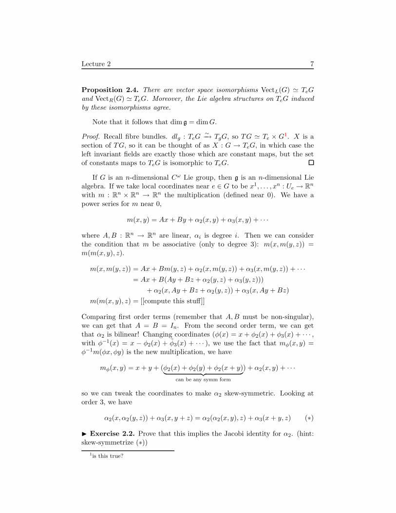
Proposition 2.4. There are vector space isomorphisms VectL(G) ≃ TeGand VectR(G) ≃ TeG. Moreover, the Lie algebra structures on TeG inducedby these isomorphisms agree.
Note that it follows that dim g = dimG.
Proof. Recall fibre bundles. dlg : TeG∼−→ TgG, so TG ≃ Te × G1. X is a
section of TG, so it can be thought of as X : G → TeG, in which case theleft invariant fields are exactly those which are constant maps, but the setof constants maps to TeG is isomorphic to TeG.
If G is an n-dimensional Cω Lie group, then g is an n-dimensional Liealgebra. If we take local coordinates near e ∈ G to be x1, . . . , xn : Ue → Rn
with m : Rn × Rn → Rn the multiplication (defined near 0). We have apower series for m near 0,
m(x, y) = Ax+By + α2(x, y) + α3(x, y) + · · ·
where A,B : Rn → Rn are linear, αi is degree i. Then we can considerthe condition that m be associative (only to degree 3): m(x,m(y, z)) =m(m(x, y), z).
m(x,m(y, z)) = Ax+Bm(y, z) + α2(x,m(y, z)) + α3(x,m(y, z)) + · · ·= Ax+B(Ay +Bz + α2(y, z) + α3(y, z)))
+ α2(x,Ay +Bz + α2(y, z)) + α3(x,Ay +Bz)
m(m(x, y), z) = [[compute this stuff]]
Comparing first order terms (remember that A,B must be non-singular),we can get that A = B = In. From the second order term, we can getthat α2 is bilinear! Changing coordinates (φ(x) = x+ φ2(x) + φ3(x) + · · · ,with φ−1(x) = x − φ2(x) + φ3(x) + · · · ), we use the fact that mφ(x, y) =φ−1m(φx, φy) is the new multiplication, we have
mφ(x, y) = x+ y + (φ2(x) + φ2(y) + φ2(x+ y)︸ ︷︷ ︸
can be any symm form
) + α2(x, y) + · · ·
so we can tweak the coordinates to make α2 skew-symmetric. Looking atorder 3, we have
α2(x, α2(y, z)) + α3(x, y + z) = α2(α2(x, y), z) + α3(x+ y, z) (∗)
Exercise 2.2. Prove that this implies the Jacobi identity for α2. (hint:skew-symmetrize (∗))
1is this true?

Lecture 2 8
Remarkably, the Jacobi identity is the only obstruction to associativity;all other coefficients can be eliminated by coordinate changes.
Example 2.5. Let G be the set of matrices of the form(a b0 a−1
)for a, b real,
a > 0. Use coordinates x, y where ex = a, y = b, then
m((x, y), (x′, y′)) = (x+ x′, exy′ + ye−x′
)
= (x+ x′, y + y′ + (xy′ − x′y︸ ︷︷ ︸
skew
) + · · · ).
The second order term is skew symmetric, so these are good coordinates.There areH,E ∈ TeG corresponding to x and y respectively so that [H,E] =E2.
Exercise 2.3. Think about this. If a, b commute, then eaeb = ea+b. Ifthey do not commute, then eaeb = ef(a,b). Compute f(a, b) to order 3.
2what does this part mean?

Lecture 3 9
Lecture 3
Last time we saw how to get a Lie algebra Lie(G) from a Lie group G.
Lie(G) = VectL(G) ≃ VectR(G).
Let x1, ..., xn be local coordinates near e ∈ G, and let m(x, y)i be theith coordinate of (x, y) 7→ m(x, y). In this local coordinate system,m(x, y)i = xi + yi + 1
2
∑cijkx
jyk + · · · . If e1, ..., en ∈ TeG is the basis
induced by x1, ..., xn, (ei ∼ ∂i), then
[ei, ej ] =∑
k
ckijek.
Example 3.1. Let G be GLn, and let (gij) be coordinates. Let X : GLn →TGLn be a vector field.
LX(f)(g) =∑
i,j
Xij(g)∂f(g)
∂gij
, where LX(l∗h(f))(g) =
lh : g 7→ hgl∗h(f)(g) = f(h−1g)
=∑
i,j
Xij(g)∂f(h−1g)
∂gij=∑
i,j
Xij(g)∂(h−1g)kl∂gij
∂f(x)
∂xkl|x=h−1g
= 〈∂(h−1g)kl∂gij
=∑
m
(h−1)km∂gml∂gij︸ ︷︷ ︸
=δimδlj
= (h−1)kiδjl〉
=∑
i,j,k
Xij(g)(h−1)ki
∂f
∂xkj|x=h−1g
=∑
j,k
(∑
i
(h−1)kiXij(g)
)
∂f
∂xkj|x=h−1g
If we want X to be left invariant,∑
i(h−1)kiXij(g) = Xkj(h
−1g), thenLX(l∗h(f)) = l∗h(LX(f)), (left invariance of X).
Example 3.2. All solutions areXij(g) = (g·M)ij , M -constant n×nmatrix.gives that left invariant vector fields on GLn ≈ n × n matrices = gln. The“Natural Basis” is eij = (Eij), Lij =
∑
m(g)mj∂
∂gmi.
Example 3.3. Commutation relations between Lij are the same as com-mutation relations between eij .
Lecture 3 10
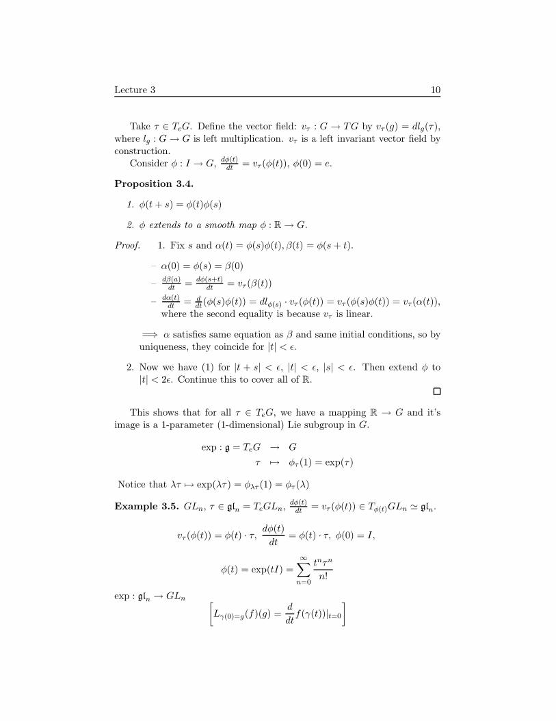
Take τ ∈ TeG. Define the vector field: vτ : G → TG by vτ (g) = dlg(τ),where lg : G→ G is left multiplication. vτ is a left invariant vector field byconstruction.
Consider φ : I → G, dφ(t)dt = vτ (φ(t)), φ(0) = e.
Proposition 3.4.
1. φ(t+ s) = φ(t)φ(s)
2. φ extends to a smooth map φ : R→ G.
Proof. 1. Fix s and α(t) = φ(s)φ(t), β(t) = φ(s+ t).
– α(0) = φ(s) = β(0)
– dβ(a)dt = dφ(s+t)
dt = vτ (β(t))
– dα(t)dt = d
dt(φ(s)φ(t)) = dlφ(s) · vτ (φ(t)) = vτ (φ(s)φ(t)) = vτ (α(t)),where the second equality is because vτ is linear.
=⇒ α satisfies same equation as β and same initial conditions, so byuniqueness, they coincide for |t| < ǫ.
2. Now we have (1) for |t + s| < ǫ, |t| < ǫ, |s| < ǫ. Then extend φ to|t| < 2ǫ. Continue this to cover all of R.
This shows that for all τ ∈ TeG, we have a mapping R → G and it’simage is a 1-parameter (1-dimensional) Lie subgroup in G.
exp : g = TeG → G
τ 7→ φτ (1) = exp(τ)
Notice that λτ 7→ exp(λτ) = φλτ (1) = φτ (λ)
Example 3.5. GLn, τ ∈ gln = TeGLn,dφ(t)dt = vτ (φ(t)) ∈ Tφ(t)GLn ≃ gln.
vτ (φ(t)) = φ(t) · τ, dφ(t)
dt= φ(t) · τ, φ(0) = I,
φ(t) = exp(tI) =
∞∑
n=0
tnτn
n!
exp : gln → GLn [
Lγ(0)=g(f)(g) =d
dtf(γ(t))|t=0
]
Lecture 3 11
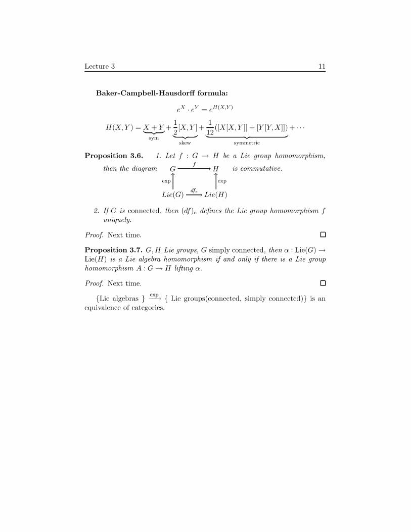
Baker-Campbell-Hausdorff formula:
eX · eY = eH(X,Y )
H(X,Y ) = X + Y︸ ︷︷ ︸
sym
+1
2[X,Y ]︸ ︷︷ ︸
skew
+1
12([X[X,Y ]] + [Y [Y,X]])
︸ ︷︷ ︸
symmetric
+ · · ·
Proposition 3.6. 1. Let f : G → H be a Lie group homomorphism,
then the diagram Gf
//OO
exp
HOO
exp
Lie(G)dfe
// Lie(H)
is commutative.
2. If G is connected, then (df)e defines the Lie group homomorphism funiquely.
Proof. Next time.
Proposition 3.7. G,H Lie groups, G simply connected, then α : Lie(G) →Lie(H) is a Lie algebra homomorphism if and only if there is a Lie grouphomomorphism A : G→ H lifting α.
Proof. Next time.
Lie algebras exp−−→ Lie groups(connected, simply connected) is anequivalence of categories.
Lecture 4 12
Lecture 4
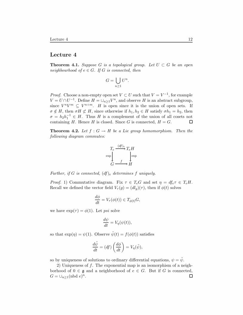
Theorem 4.1. Suppose G is a topological group. Let U ⊂ G be an openneighbourhood of e ∈ G. If G is connected, then
G =⋃
n≥1
Un.
Proof. Choose a non-empty open set V ⊂ U such that V = V −1, for exampleV = U ∩U−1. Define H = ∪n≥1V
n, and observe H is an abstract subgroup,since V nV m ⊆ V n+m. H is open since it is the union of open sets. Ifσ /∈ H, then σH 6⊂ H, since otherwise if h1, h2 ∈ H satisfy σh1 = h2, thenσ = h2h
−11 ∈ H. Thus H is a complement of the union of all cosets not
containing H. Hence H is closed. Since G is connected, H = G.
Theorem 4.2. Let f : G → H be a Lie group homomorphism. Then thefollowing diagram commutes:
Te(df)e
//
exp
TeH
exp
Gf
// H
Further, if G is connected, (df)e determines f uniquely.
Proof. 1) Commutative diagram. Fix τ ∈ TeG and set η = dfeτ ∈ TeH.Recall we defined the vector field Vτ (g) = (dlg)(τ), then if φ(t) solves
dφ
dt= Vτ (φ(t)) ∈ Tφ(t)G,
we have exp(τ) = φ(1). Let psi solve
dψ
dt= Vη(ψ(t)),
so that exp(η) = ψ(1). Observe ψ(t) = f(φ(t)) satisfies
dψ
dt= (df)
(dφ
dt
)
= Vη(ψ),
so by uniqueness of solutions to ordinary differential equations, ψ = ψ.2) Uniqueness of f . The exponential map is an isomorphism of a neigh-
borhood of 0 ∈ g and a neighborhood of e ∈ G. But if G is connected,G = ∪n≥1(nbd e)n.

Lecture 4 13
Theorem 4.3. Suppose G is a topological group, with G0 ⊂ G the connectedcomponent of e. Then 1) G0 is normal and 2) G/G0 is discrete.
Proof. 2) G0 ⊂ G is open implies pr−1([e]) = eG0 is open in G, which inturn implies pr−1([g]) ∈ G/G0 is open for every g ∈ G. Thus each coset isboth open and closed, hence G/G0 is discrete.
1) Fix g ∈ G and consider the map G→ G defined by x 7→ gxg−1. Thismap fixes e and is continuous, which implies it maps G0 into G0. In otherwords, gG0g−1 ⊂ G0, or G0 is normal.
We recall some basic notions of algebraic topology. Suppose M is aconnected topological space. Let x, y ∈ M , and suppose γ(t) : [0, 1] → Mis a path from x to y in M . We say γ(t) is homotopic to γ if there is acontinuous map h(s, t) : [0, 1]2 →M satisfying
•h(s, 0) = x, h(s, 1) = y
•h(0, t) = γ(t), h(1, t) = γ(t).
We call h the homotopy. On a smooth manifold, we may replace h with asmooth homotopy. Now fix x0 ∈M . We define the first fundamental groupof M
π1(M,x0) = homotopy classes of loops based at x0 .
It is clear that this is a group with group multiplication composition ofpaths. It is also a fact that the definition does not depend on the base pointx0:
π1(M,x0) ≃ π1(M,x′0).
By π1(M) we denote the isomorphism class of π1(M, ·). Lastly, we say M issimply connected if π1(M) = e, that is if all closed paths can be deformedto the trivial one.
Theorem 4.4. Suppose G and H are Lie groups with Lie algebras g, hrespectively. If G is simply connected, then any Lie algebra homomorphismρ : g → h lifts to a Lie group homomorphism R : G→ H.
In order to prove this theorem, we will need the following lemma.
Lemma 4.5. Let ξ : R→ g be a smooth mapping. Then
dg
dt= (dlg)(ξ(t))
has a unique solution on all of R with g(t0) = g0.

Lecture 4 14
For convenience, we will write gξ := (dlg)(ξ).
Proof. Since g is a vector space, we identify it with Rn and for sufficientlysmall r > 0, we identify Br(0) ⊂ g with a small neighbourhood of e, Ue(r) ⊂G, under the exponential map. Here Br(0) is measured with the usualEuclidean norm ‖ · ‖. Note for any g ∈ Ue(r) and |t− t0| sufficiently small,we have ‖gξ(t)‖ ≤ C. Now according to Exercise 4.1, the solution withg(t0) = e exists for sufficiently small |t− t0| and
g(t) ∈ Ue(r) ∀|t− t0| <r
C ′ .
Now define h(t) = g(t)g0 so that h(t) ∈ Ug0(r) for |t− t0| < r/C ′. That is, rand C ′ do not depend on the choice of initial conditions, and we can coverR by intervals of length, say r/C ′.
Exercise 4.1. Verify that there is a constant C ′ such that if |t − t0| issufficiently small, we have
‖g(t)‖ ≤ C ′|t− t0|.
Proof of Theorem 4.4. We will construct R : G→ H. Beginning with g(t) :[0, 1] → G satisfying g(0) = e, g(1) = g, define ξ(t) ∈ g for each t by
g(t)ξ(t) =d
dtg(t).
Let η(t) = ρ(ξ(t)), and let h(t) : [0, 1] → H satisfy
d
dth(t) = h(t)η(t), h(0) = e.
Define R(g) = h(1).Claim: h(1) does not depend on the path g(t), only on g.
Proof of Claim. Suppose g1(t) and g2(t) are two different paths connectinge to g. Then there is a smooth homotopy g(t, s) satisfying g(t, 0) = g1(t),g(t, 1) = g2(t). Define ξ(t, s) and η(t, s) by
∂g
∂t= g(t, s)ξ(t, s);
∂g
∂s= g(t, s)η(t, s).
Observe
∂2g
∂s∂t= gη ξ + g
∂ξ
∂tand (1)
∂2g
∂t∂s= gξ η + g
∂η
∂s, (2)
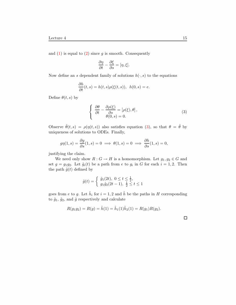
Lecture 4 15
and (1) is equal to (2) since g is smooth. Consequently
∂η
∂t− ∂ξ
∂s= [η, ξ].
Now define an s dependent family of solutions h(·, s) to the equations
∂h
∂t(t, s) = h(t, s)ρ(ξ(t, s)), h(0, s) = e.
Define θ(t, s) by
∂θ
∂t− ∂ρ(ξ)
∂s= [ρ(ξ), θ] ,
θ(0, s) = 0.(3)
Observe θ(t, s) = ρ(η(t, s)) also satisfies equation (3), so that θ = θ byuniqueness of solutions to ODEs. Finally,
gη(1, s) =∂g
∂s(1, s) = 0 =⇒ θ(1, s) = 0 =⇒ ∂h
∂s(1, s) = 0,
justifying the claim.We need only show R : G→ H is a homomorphism. Let g1, g2 ∈ G and
set g = g1g2. Let gi(t) be a path from e to gi in G for each i = 1, 2. Thenthe path g(t) defined by
g(t) =
g1(2t), 0 ≤ t ≤ 1
2 ,g1g2(2t− 1), 1
2 ≤ t ≤ 1
goes from e to g. Let hi for i = 1, 2 and h be the paths in H correspondingto g1, g2, and g respectively and calculate
R(g1g2) = R(g) = h(1) = h1(1)h2(1) = R(g1)R(g2).

Lecture 5 16
Lecture 5
Last time we talked about connectedness, and proved the following things:
- Any connected topological group G has the property that G =⋃
n Vn,
where V is any neighborhood of e ∈ G.
- If G is a connected Lie group, with α : Lie(G) → Lie(H) a Lie algebrahomomorphism, then if there exists f : G → H with dfe = α, it isunique.
- If G is connected, simply connected, with α : Lie(G) → Lie(H) a Liealgebra homomorphism, then there is a unique f : G → H such thatdfe = α.
Simply Connected Lie Groups
The map p in Z → Xp−→ Y is a covering map if it is a locally trivial fiber
bundle with discrete fiber Z. Locally trivial means that for any y ∈ Y thereis a neighborhood U such that if f : U × Z → Z is the map defined byf(u, z) = u, then the following diagram commutes:
p−1U
≃ U × Z
fyyttttttttttt
Y ⊇ U
The exact sequence defined below is an important tool. Suppose wehave a locally trivial fiber bundle with fiber Z (not necessarily discrete),with X,Y connected. Choose x0 ∈ X, z0 ∈ Z, y0 ∈ Y such that p(x0) = y0,and i : Z → p−1(y0) is an isomorphism such that i(z0) = x0:
x0 ∈ π−1(y0)
Zioo
y0
We can define p∗ : π1(X,x0) → π1(Y, y0) in the obvious way (π1 is a functor).Also define i∗ : π1(Z, z0) → π1(X,x0). Then we can define ∂ : π1(Y, y0) →π0(Z) = connected components of Z by taking a loop γ based at y0 andlifting it to some path γ. This path is not unique, but up to fiber-preservinghomotopy it is. The new path γ starts at x0 and ends at x′0. Then we define∂ to be the map associating the connected component of x′0 to the homotopyclass of γ.
Lecture 5 17
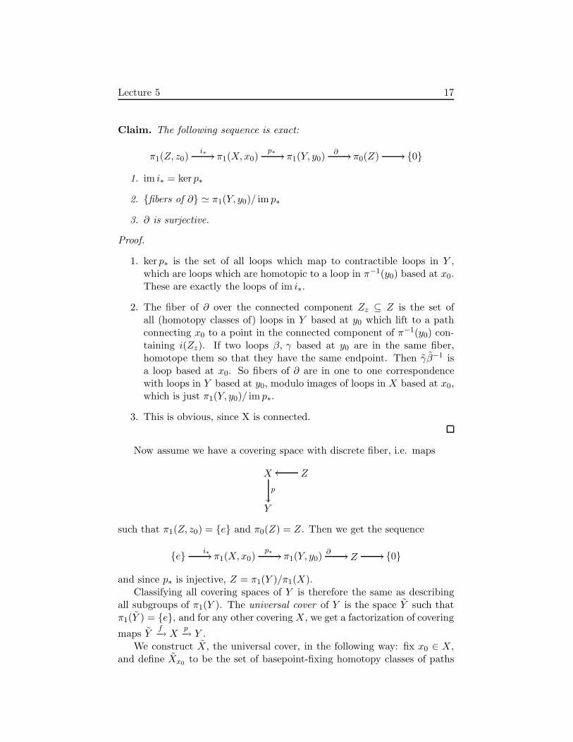
Claim. The following sequence is exact:
π1(Z, z0)i∗ // π1(X,x0)
p∗// π1(Y, y0)
∂ // π0(Z) // 0
1. im i∗ = ker p∗
2. fibers of ∂ ≃ π1(Y, y0)/ im p∗
3. ∂ is surjective.
Proof.
1. ker p∗ is the set of all loops which map to contractible loops in Y ,which are loops which are homotopic to a loop in π−1(y0) based at x0.These are exactly the loops of im i∗.
2. The fiber of ∂ over the connected component Zz ⊆ Z is the set ofall (homotopy classes of) loops in Y based at y0 which lift to a pathconnecting x0 to a point in the connected component of π−1(y0) con-taining i(Zz). If two loops β, γ based at y0 are in the same fiber,homotope them so that they have the same endpoint. Then γβ−1 isa loop based at x0. So fibers of ∂ are in one to one correspondencewith loops in Y based at y0, modulo images of loops in X based at x0,which is just π1(Y, y0)/ im p∗.
3. This is obvious, since X is connected.
Now assume we have a covering space with discrete fiber, i.e. maps
X
p
Zoo
Y
such that π1(Z, z0) = e and π0(Z) = Z. Then we get the sequence
e i∗ // π1(X,x0)p∗
// π1(Y, y0)∂ // Z // 0
and since p∗ is injective, Z = π1(Y )/π1(X).Classifying all covering spaces of Y is therefore the same as describing
all subgroups of π1(Y ). The universal cover of Y is the space Y such thatπ1(Y ) = e, and for any other covering X, we get a factorization of covering
maps Yf−→ X
p−→ Y .We construct X, the universal cover, in the following way: fix x0 ∈ X,
and define Xx0 to be the set of basepoint-fixing homotopy classes of paths
Lecture 5 18
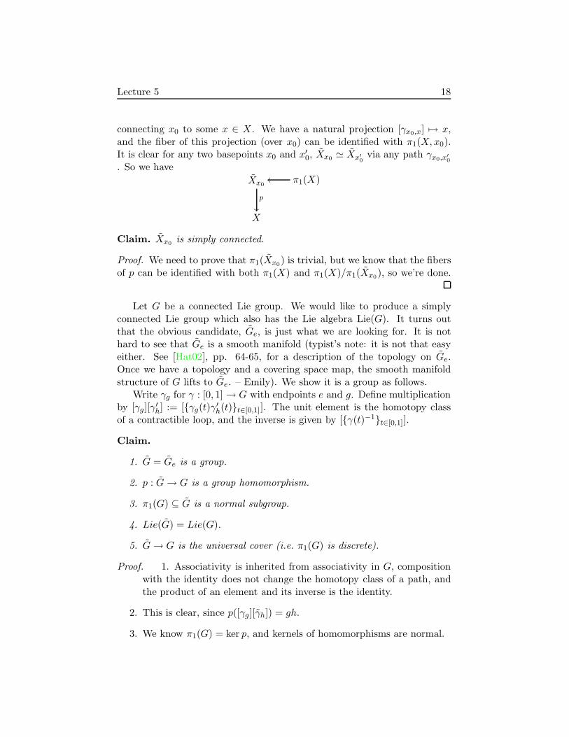
connecting x0 to some x ∈ X. We have a natural projection [γx0,x] 7→ x,and the fiber of this projection (over x0) can be identified with π1(X,x0).It is clear for any two basepoints x0 and x′0, Xx0 ≃ Xx′0
via any path γx0,x′0. So we have
Xx0
p
π1(X)oo
X
Claim. Xx0 is simply connected.
Proof. We need to prove that π1(Xx0) is trivial, but we know that the fibersof p can be identified with both π1(X) and π1(X)/π1(Xx0), so we’re done.
Let G be a connected Lie group. We would like to produce a simplyconnected Lie group which also has the Lie algebra Lie(G). It turns outthat the obvious candidate, Ge, is just what we are looking for. It is nothard to see that Ge is a smooth manifold (typist’s note: it is not that easyeither. See [Hat02], pp. 64-65, for a description of the topology on Ge.Once we have a topology and a covering space map, the smooth manifoldstructure of G lifts to Ge. – Emily). We show it is a group as follows.
Write γg for γ : [0, 1] → G with endpoints e and g. Define multiplicationby [γg][γ
′h] := [γg(t)γ′h(t)t∈[0,1]]. The unit element is the homotopy class
of a contractible loop, and the inverse is given by [γ(t)−1t∈[0,1]].
Claim.
1. G = Ge is a group.
2. p : G→ G is a group homomorphism.
3. π1(G) ⊆ G is a normal subgroup.
4. Lie(G) = Lie(G).
5. G→ G is the universal cover (i.e. π1(G) is discrete).
Proof. 1. Associativity is inherited from associativity in G, compositionwith the identity does not change the homotopy class of a path, andthe product of an element and its inverse is the identity.
2. This is clear, since p([γg][γh]) = gh.
3. We know π1(G) = ker p, and kernels of homomorphisms are normal.

Lecture 5 19
4. The topology on G is induced by the topology of G in the followingway: If U is a basis for the topology on G then fix a path γe,g for allg ∈ G. Then U = Uγe,g is a basis for the topology on G with Uγe,g
defined to be the set of paths of the form γ−1e,gβγe,g with β a loop based
at g contained entirely in U .
Now take U a connected, simply connected neighborhood of e ∈ G.Since all paths in U from e to a fixed g ∈ G are homotopic, we havethat U and U are diffeomorphic and isomorphic, hence Lie isomorphic.Thus Lie(G) = Lie(G).
5. As established in (4), G and G are diffeomorphic in a neighborhoodof the identity. Thus all points x ∈ p−1(e) have a neighborhood whichdoes not contain any other inverse images of e, so p−1(e) is discrete;and p−1(e) and π1(G) are isomorphic.
We have that for any Lie group G with a given Lie algebra Lie(G) = g,there exists a simply connected Lie group G with the same Lie algebra, andG is the universal cover of G.
Lemma 5.1. A discrete normal subgroup H ⊆ G of a connected topologicalgroup G is always central.
Proof. Consider the map φh : G → H, g 7→ ghg−1h−1, which is continuous.Since G is connected, the image is also connected, but H is discrete, so theimage must be a point. In fact, it must be e because φh(h) = e. So H iscentral.
Corollary 5.2. π1(G) is central, because it is normal and discrete. Inparticular, π1(G) is commutative.
Corollary 5.3. G ≃ G/π1(G), with π1(G) discrete central.
The following corollary describes all (connected) Lie groups with a givenLie algebra.
Corollary 5.4. Given a Lie algebra g, take G with Lie algebra g. Then anyother connected G with Lie algebra g is a quotient of G by a discrete centralsubgroup of G.
Suppose G is a topological group and G0 is a connected component of e.
Claim. G0 ⊆ G is a normal subgroup, and G/G0 is a discrete group.
Lecture 5 20
If we look at Lie groups → Lie algebras, we have an “inverse” givenby exponential: exp(g) ⊆ G. Then G0 =
⋃
n(exp g)n. So for a given Liealgebra, we can construct a well-defined isomorphism class of connected,simply connected Lie groups. When we say “take a Lie group with this Liealgebra”, we mean to take the connected, simply connected one.
Coming Attractions: We will talk about Ug, the universal envelopingalgebra, C(G), the Hopf algebra, and then we’ll do classification of Liealgebras.
Lecture 6 - Hopf Algebras 21
Lecture 6 - Hopf Algebras
Last time: We showed that a finite dimensional Lie algebra g uniquely deter-mines a connected simply connected Lie group. We also have a “map” in theother direction (taking tangent spaces). So we have a nice correspondencebetween Lie algebras and connected simply connected Lie groups.
There is another nice kind of structure: Associative algebras. How dothese relate to Lie algebras and groups?
Let Γ be a finite group and let C[Γ] := ∑
g cgg|g ∈ Γ, cg ∈ C be theC vector space with basis Γ. We can make C[Γ] into an associative algebraby taking multiplication to be the multiplication in Γ for basis elements andlinearly extending this to the rest of C[Γ].1
Remark 6.1. Recall that the tensor product V and W is the linear span ofelements of the form v ⊗ w, modulo some linearity relations. If V and Ware infinite dimensional, we will look at the algebraic tensor product of Vand W , i.e. we only allow finite sums of the form
∑ai ⊗ bi.
We have the following maps
Comultiplication: ∆ : C[Γ] → C[Γ] ⊗ C[Γ], given by ∆(∑xgg) =
∑xgg ⊗ g
Counit: ε : C[Γ] → C, given by ε(∑xgg) =
∑xg.
Antipode: S : C[Γ] → C[Γ] given by S(∑xgg) =
∑xgg
−1.
You can check that
– ∆(xy) = ∆(x)∆(y) (i.e. ∆ is an algebra homomorphism),
– (∆ ⊗ Id) ∆ = (Id ⊗ ∆) ∆. (follows from the associativity of ⊗),
– ε(xy) = ε(x)ε(y) (i.e. ε is an algebra homomorphism),
– S(xy) = S(y)S(x) (i.e. S is an algebra antihomomorphism).
Consider
C[Γ]∆−→ C[Γ] ⊗ C[Γ]
S⊗Id,Id⊗S−−−−−−−→ C[Γ] ⊗ C[Γ]m−→ C[Γ].
You getm(S ⊗ Id)∆(g) = m(g−1 ⊗ g) = e
so the composition sends∑xgg to (
∑
g xg)e = ε(x)1A.So we have
1“If somebody speaks Danish, I would be happy to take lessons.”
Lecture 6 - Hopf Algebras 22
1. A = C[Γ] an associative algebra with 1A
2. ∆ : A → A ⊗ A which is coassociative and is a homomorphism ofalgebras
3. ε : A→ C an algebra homomorphism, with (ε⊗Id)∆ = (Id⊗ε)∆ = Id.
Definition 6.2. Such an A is called a bialgebra, with comultiplication ∆and counit ε.
We also have S, the antipode, which is an algebra anti-automorphism,so it is a linear isomorphism with S(ab) = S(b)S(a), such that
A⊗AS⊗Id
Id⊗S// A⊗A
m
A
∆
OO
ε // C1A // A
Definition 6.3. A bialgebra with an antipode is a Hopf algebra.
If A is finite dimensional, let A∗ be the dual vector space. Define themultiplication, ∆∗, S∗, ε∗, 1A∗ on A∗ in the following way:
– lm(a) := (l ⊗m)(∆a) for all l,m ∈ A∗
– ∆∗(l)(a⊗ b) := l(ab)
– S∗(l)(a) := l(S(a))
– ε∗(l) := l(1A)
– 1A∗(a) := ε(a)
Theorem 6.4. A∗ is a Hopf algebra with this structure, and we say it isdual to A. If A is finite-dimensional, then A∗∗ = A.
Exercise 6.1. Prove it.
We have an example of a Hopf algebra (C[Γ]), what is the dual Hopfalgebra?2 Let’s compute A∗ = C[Γ]∗.
Well, C[Γ] has a basis g ∈ Γ. Let δg be the dual basis, so δg(h) = 0if g 6= h and 1 if g = h. Let’s look at how we multiply such things
– δg1δg2(h) = (δg1 ⊗ δg2)(h ⊗ h) = δg1(h)δg2(h).
– ∆∗(δg)(h1 ⊗ h2) = δg(h1h2)
2 If you want to read more, look at S. Montgomery’s Hopf algebras, AMS, early 1990s.[Mon93]
Lecture 6 - Hopf Algebras 23
– S∗(δg)(h) = δg(h−1)
– ε∗(δg) = δg(e) = δg,e
– 1A∗(h) = 1.
It is natural to think of A∗ as the set of functions Γ → C, where(∑xgδg)(h) =
∑xgδg(h). Then we can think about functions
– (f1f2)(h) = f1(h)f2(h)
– ∆∗(f)(h1 × h2) = f(h1h2)
– S∗(f)(h) = f(h−1)
– ε∗(f) = f(e)
– 1A∗ = 1 constant.
So this is the Hopf algebra C(Γ), the space of functions on Γ. If Γ is any affinealgebraic group, then C(Γ) is the space of polynomial functions on Γ, and allthis works. The only concern is that we need C(Γ×Γ) ∼= C(Γ)⊗C(Γ), whichwe only have in the finite dimensional case; you have to take completions oftensor products otherwise.
So we have the notion of a bialgebra (and duals), and the notion of aHopf algebra (and duals). We have two examples: A = C[Γ] and A∗ = C(Γ).A natural question is, “what if Γ is an infinite group or a Lie group?” and“what are some other examples of Hopf algebras?”
Let’s look at some infinite dimensional examples. If A is an infinitedimensional Hopf algebra, and A⊗A is the algebraic tensor product (finitelinear combinations of formal a ⊗ b s). Then the comultiplication shouldbe ∆ : A → A ⊗ A. You can consider cases where you have to take somecompletion of the tensor product with respect to some topology, but wewon’t deal with this kind of stuff. In this case, A∗ is too big, so instead ofthe notion of the dual Hopf algebra, we have dual pairs.
Definition 6.5. A dual pairing of Hopf algebras A and H is a pair with abilinear map 〈 , 〉 : A⊗H → C which is nondegenerate such that
(1) 〈∆a, l ⊗m〉 = 〈a, lm〉
(2) 〈ab, l〉 = 〈a⊗ b,∆∗l〉
(3) 〈Sa, l〉 = 〈a, S∗l〉
(4) ε(a) = 〈a, 1H〉, εH (l) = 〈1A, l〉
Lecture 6 - Hopf Algebras 24
Exmaple: A = C[x], then what is A∗? You can evaluate a polynomial at0, or you can differentiate some number of times before you evaluate at 0.A∗ = span of linear functionals on polynomial functions of C of the form
ln(f) =
(d
dx
)n
f(x)∣∣x=0
.
A basis for C[x] is 1, xn with n ≥ 1, and we have
ln(xm) =
m! , n = m0 , n 6= m
What is the Hopf algebra structure on A? We already have an algebrawith identity. Define ∆(x) = x ⊗ 1 + 1 ⊗ x and extend it to an algebrahomomorphism, then it is clearly coassociative. Define ε(1) = 1 and ε(xn) =0 for all n ≥ 1. Define S(x) = −x, and extend to an algebra homomorphism.It is easy to check that this is a Hopf algebra.
Let’s compute the Hopf algebra structure on A∗. We have
lnlm(xN ) = (ln ⊗ lm)(∆(xN ))
= (ln ⊗ lm)(∑
(N
k
)
xN−k ⊗ xk)
Exercise 6.2. Compute this out. The answer is that A∗ = C[y = ddx ],
and the Hopf algebra structure is the same as A.
This is an example of a dual pair: A = C[x],H = C[y], with 〈xn, ym〉 =δn,mm!.
Summary: If A is finite dimensional, you get a dual, but in the infinitedimensional case, you have to use dual pairs.
The universal enveloping algebra
The idea is to construct a map from Lie algebras to associative algebras sothat the representation theory of the associative algebra is equivalent to therepresentation theory of the Lie algebra.
1) let V be a vector space, then we can form the free associative algebra(or tensor algebra) of V : T (V ) = C ⊕ (⊕n≥1V
⊗n). The multiplication isgiven by concatenation: (v1 ⊗ · · · ⊗ vn) · (w1 ⊗ · · · ⊗ wm) = v1 ⊗ · · · ⊗ vn ⊗w1 ⊗ · · ·wm. It is graded: Tn(V )Tm(V ) ⊆ Tn+m(V ). It is also a Hopfalgebra, with ∆(x) = x ⊗ 1 + 1 ⊗ x, S(x) = −x, ε(1) = 1 and ε(x) = 0. Ifyou choose a basis e1, . . . , en of V , then T (V ) is the free associative algebra〈e1, . . . , en〉. This algebra is Z+-graded: T (V ) = ⊕n≥0Tn(V ), where thedegree of 1 is zero and the degree of each ei is 1. It is also a Z-gradedbialgebra: ∆(Tn(V )) ⊆ ⊕(Ti ⊕ Tn−i), S(Tn(V )) ⊂ Tn(V ), ε : T (V ) → C is amapping of graded spaces ((C)n = 0).
Lecture 6 - Hopf Algebras 25
Definition 6.6. Let A be a Hopf algebra. Then a two-sided ideal I ⊆ A isa Hopf ideal if ∆(I) ⊆ A⊗ I + I ⊗A, S(I) = I, and ε(I) = 0.
You can check that the quotient of a Hopf algebra by a Hopf ideal isa Hopf algebra (and that the kernel of a map of Hopf algebras is always aHopf ideal).
Exercise 6.3. Show that I0 = 〈v⊗w−w⊗ v|v,w ∈ V = T1(V ) ⊆ T (V )〉is a homogeneous Hopf ideal.
Corollary 6.7. S(V ) = T (V )/I0 is a graded Hopf algebra.
Choose a basis e1, . . . , en in V , so that T (V ) = 〈e1, . . . , en〉 and S(V ) =〈e1, . . . , en〉/〈eiej − ejei〉
Exercise 6.4. Prove that the Hopf algebra S(V ) is isomorphic to C[e1]⊗· · · ⊗C[en].
Remark 6.8. From the discussion of C[x], we know that S(V ) and S(V ∗)are dual.
Exercise 6.5. Describe the Hopf algebra structure on T (V ∗) that isdetermined by the pairing 〈v1⊗· · ·⊗vn, l1⊗· · ·⊗ lm〉 = δm,nl1(v1) · · · ln(vn).(free coalgebra of V ∗)
Now assume that g is a Lie algebra.
Definition 6.9. The universal enveloping algebra of g is U(g) = T (g)/〈x⊗y − y ⊗ x− [x, y]〉.
Exercise: prove that 〈x⊗ y − y ⊗ x− [x, y]〉 is a Hopf ideal.
Corollary 6.10. Ug is a Hopf algebra.
If e1, . . . , en is a basis for V . Ug = 〈e1, . . . , en|eiej − ejei =∑
k ckijek〉,
where ckij are the structure constants of [ , ].
Remark 6.11. The ideal 〈eiej−ejei〉 is homogeneous, but 〈x⊗y−y⊗x−[x, y]〉is not, so Ug isn’t graded, but it is filtered.
Lecture 7 26
Lecture 7
Last time we talked about Hopf algebras. Our basic examples were C[Γ]and C(Γ) = C[Γ]∗. Also, for a vector space V , T (V ) is a Hopf algebra.Then S(V ) = T (V )/〈x ⊗ y − y ⊗ x|x, y ∈ V 〉. And we also have Ug =Tg/〈x⊗ y − y ⊗ x− [x, y]|x, y ∈ g〉.
Today we’ll talk about the universal enveloping algebra. Later, we’lltalk about deformations of associative algebras because that is where recentprogress in representation theory has been.
Universality of Ug
We have that g → Tg → Ug. And σ : g → Ug canonical embedding(of vector spaces and Lie algebras). Let A be an associative algebra withτ : g → L(A) = A|[a, b] = ab− ba a Lie algebra homomorphism such thatτ([x, y]) = τ(x)τ(y) − τ(y)τ(x).
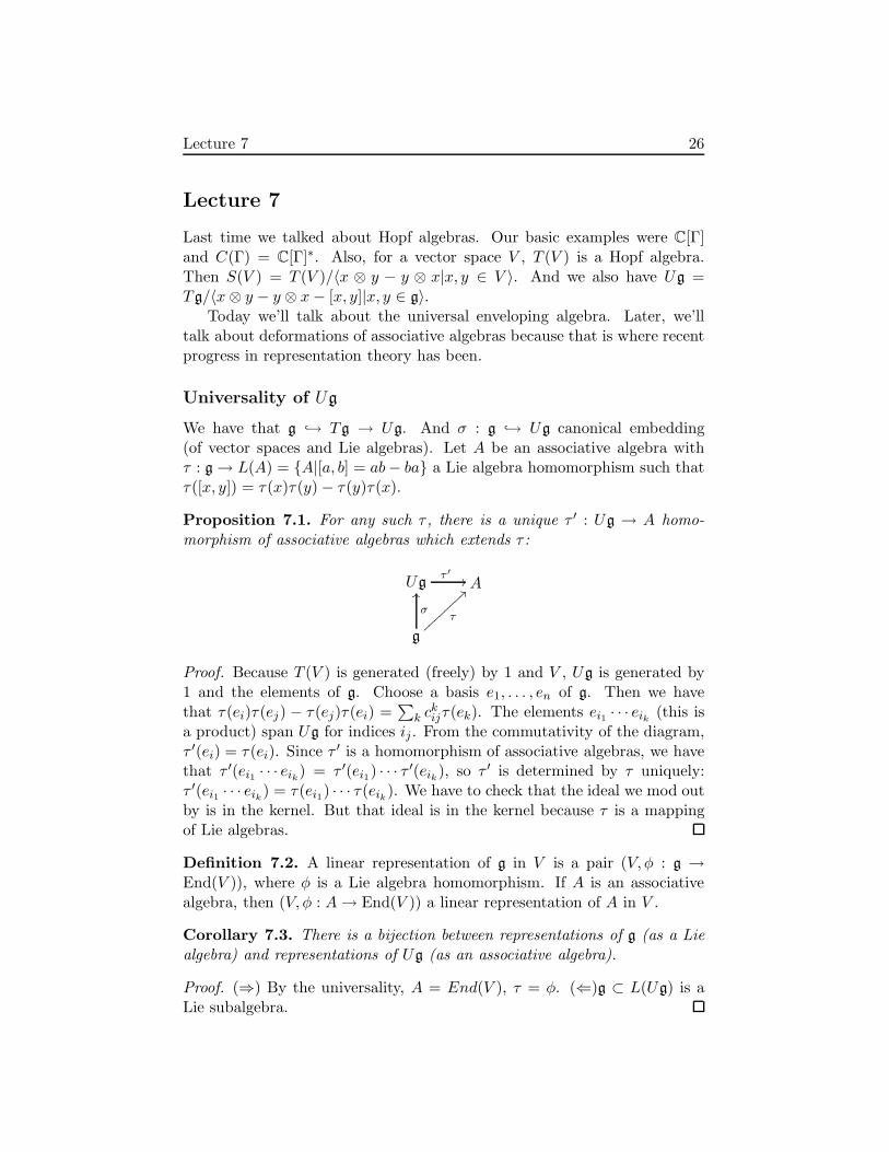
Proposition 7.1. For any such τ , there is a unique τ ′ : Ug → A homo-morphism of associative algebras which extends τ :
Ugτ ′ // A
g
σ
OO
τ
>>
Proof. Because T (V ) is generated (freely) by 1 and V , Ug is generated by1 and the elements of g. Choose a basis e1, . . . , en of g. Then we havethat τ(ei)τ(ej) − τ(ej)τ(ei) =
∑
k ckijτ(ek). The elements ei1 · · · eik (this is
a product) span Ug for indices ij . From the commutativity of the diagram,τ ′(ei) = τ(ei). Since τ ′ is a homomorphism of associative algebras, we havethat τ ′(ei1 · · · eik) = τ ′(ei1) · · · τ ′(eik), so τ ′ is determined by τ uniquely:τ ′(ei1 · · · eik) = τ(ei1) · · · τ(eik). We have to check that the ideal we mod outby is in the kernel. But that ideal is in the kernel because τ is a mappingof Lie algebras.
Definition 7.2. A linear representation of g in V is a pair (V, φ : g →End(V )), where φ is a Lie algebra homomorphism. If A is an associativealgebra, then (V, φ : A→ End(V )) a linear representation of A in V .
Corollary 7.3. There is a bijection between representations of g (as a Liealgebra) and representations of Ug (as an associative algebra).
Proof. (⇒) By the universality, A = End(V ), τ = φ. (⇐)g ⊂ L(Ug) is aLie subalgebra.

Lecture 7 27
Example 7.4 (Adjoint representation). ad : g → End g given by x :y 7→ [x, y]. This is also a representation of Ug. Let e1, . . . , en be a basis in g.Then we have that adei(ej) = [ei, ej ] =
∑
k ckijek, so the matrix representing
the adjoint action of the element ei is the matrix (adei)jk = (ckij) of struc-tural constants. You can check that ad[ei,ej ] = (adei)(adej ) − (adej )(adei)
is same as the Jacobi identity for the ckij. We get ad : Ug → End(g) bydefining it on the monomials ei1 · · · eik as adei1
···eik= (adei1
) · · · (adeik) (the
product of matrices).
Let’s look at some other properties of Ug.
Gradation in Ug
Recall that V is a Z+-graded vector space if V = ⊕∞n=0Vn. A linear map
f : V → W between graded vector spaces is grading-preserving if f(Vn) ⊆Wn. If we have a tensor product V ⊗ W of graded vector spaces, it hasa natural grading given by (V ⊗W )n = ⊕n
i=0Vi ⊗Wn−i. The “geometricmeaning” of this is that there is a linear action of C on V such that Vn =x|t(x) = tn ·x for all t ∈ C. A graded morphism is a linear map respectingthis action, and the tensor product has the diagonal action of C, given byt(x⊗ y) = t(x) ⊗ t(y).
Example 7.5. If V = C[x], ddx is not grading preserving, x d
dx is.
We say that (V, [ , ]) is a Z+-graded Lie algebra if [ , ] : V ⊗ V → V isgrading-preserving.
Example 7.6. Let V be the space of polynomial vector fields on C =Span(zn d
dz )n≥0. Then Vn = Czn ddz .
An associative algebra (V,m : V ⊗V → V ) is Z+-graded if m is grading-preserving.
Example 7.7.
(1) V = C[x], where the action of C is given by x 7→ tx.
(2) V = C[x1, . . . , xn] where the degree of each variable is 1 ... this is then-th tensor power of the previous example.
(3) Lie algebra: Vect(C) = ∑n≥0 anxn+1 d
dx with Vectn(C) = Cxn+1 ddx ,
deg(x) = 1. You can embed Vect(C) into polynomial vector fields onS1 (Virasoro algebra).
(4) T(V) is a Z+-graded associative algebra, as is S(V ). However, Ug isnot because we have modded out by a non-homogeneous ideal. Butthe ideal is not so bad. Ug is a Z+-filtered algebra:

Lecture 7 28
Filtered spaces and algebras
Definition 7.8. V is a filtered space if it has an increasing filtration
V0 ⊂ V1 ⊂ V2 ⊂ · · · ⊂ V
such that V =⋃Vi, and Vn = is a subspace of dimension less than or equal
to n. f : V →W is a morphism of filtered vector spaces if f(Vn) ⊆Wn.
We can define filtered lie algebras and associative algebras as such thatthe bracket/multiplication are filtered maps.
There is a functor from filtered vector spaces to graded associative alge-bras Gr : V → Gr(V ), where Gr(V ) = V0⊕V1/V0⊕V2/V1 · · · . If f : V → Wis filtration preserving, it induces a map Gr(f) : Gr(V ) → Gr(W ) functori-ally such that this diagram commutes:
Vf
//
Gr
W
Gr
Gr(V )Gr(f)
// Gr(W )
Let A be an associative filtered algebra (i.e. AiAj ⊆ Ai+j) such that forall a ∈ Ai, b ∈ Aj, ab− ba ∈ Ai+j−1.
Proposition 7.9. For such an A,
(1) Gr(A) has a natural structure of an associative, commutative algebra(that is, the multiplication in A defines an associative, commutativemultiplication in Gr(A)).
(2) For a ∈ Ai+1, b ∈ Aj+1, the operation aAi, bAj = aAibAj − bAjaAimod Ai+j is a lie bracket on Gr(A).
(3) x, yz = x, yz + yx, z.
Proof. Exercise1. You need to show that the given bracket is well defined,and then do a little dance, keeping track of which graded component youare in.
Definition 7.10. A commutative associative algebra B is called a Poissonalgebra if B is also a lie algebra with lie bracket , (called a Poissonbracket) such that x, yz = x, yz + yx, z (the bracket is a derivation).

Lecture 7 29
Example 7.11. Let (M,ω) be a symplectic manifold (i.e. ω is a closednon-degenerate 2-form on M), then functions on M form a Poisson algebra.We could have M = R2n with coordinates p1, . . . , pn, q1, . . . , qn, and ω =∑
i dpi ∧ dqi. Then the multiplication and addition on C∞(M) is the usual
one, and we can define f, g =∑
ij pij ∂f∂xi
∂g∂xj , where ω =
∑ωijdx
i ∧ dxjand (pij) is the inverse matrix to (ωij). You can check that this is a Poissonbracket.
Let’s look at Ug = 〈1, ei|eiej−ejei =∑
k ckijek〉. Then Ug is filtered, with
(Ug)n = Spanei1 · · · eik |k ≤ n. We have the obvious inclusion (Ug)n ⊆(Ug)n+1 and (Ug)0 = C · 1.
Proposition 7.12.
(1) Ug is a filtered algebra (i.e. (Ug)r(Ug)s ⊆ (Ug)r+s)
(2) [(Ug)r, (Ug)s] ⊆ (Ug)r+s−1.
Proof. 1) obvious. 2) Exercise2 (almost obvious).
Now we can consider Gr(Ug) = C · 1 ⊕ (⊕
r≥1(Ug)r/(Ug)r−1)
Claim. (Ug)r/(Ug)r−1 ≃ Sr(g) = symmetric elements of (C[e1, . . . , en])r.
Proof. Exercise3.
So Gr(Ug) ≃ S(g) as a commutative algebra.S(g) ∼= Polynomial functions on g∗ = HomC(g,C).Consider C∞(M). How can we construct a bracket , which satisfies
Liebniz (i.e. f, g1g2 = f, g1g2 + f, g2g1). We expect that f, g(x) =pij(x) ∂f
∂xi∂g∂xj = 〈p(x), df(x)∧ dg(x)〉. Such a p is called a bivector field (it is
a section of the bundle TM ∧TM →M). So a Poisson structure on C∞(M)is the same as a bivector field p on M satisfying the Jacobi identity. You cancheck that the Jacobi identity is some bilinear identity on pij which followsfrom the Jacobi identity on , . This is equivalent to the Schouten identity,which says that the Schouten bracket of some things vanishes [There shouldbe a reference here]. This is more general than the symplectic case becausepij can be degenerate.
Let g have the basis e1, . . . , en and corresponding coordinate functionsx1, . . . , xn. On g∗, we have that dual basis e1, . . . , en (you can identify thesewith the coordinates x1, . . . , xn), and coordinates x1, . . . , xn (which you canidentify with the ei). The bracket on polynomial functions on g∗ is given by
p, q =∑
ckijxk∂p
∂xi
∂q
∂xj.
This is a Lie bracket and clearly acts by derivations.

Lecture 7 30
Next we will study the following. If you have polynomials p, q on g∗, youcan try to construct an associative product p ∗t q = pq+ tm1(p, q)+ · · · . Wewill discuss deformations of commutative algebras. The main example willbe the universal enveloping algebra as a deformation of polynomial functionson g∗.
Lecture 8 - PBW theorem, Deformations of Associative Algebras 31
Lecture 8 - PBW theorem, Deformations of Asso-
ciative Algebras
Last time, we introduced the universal enveloping algebra Ug of a Lie algebrag, with its universality property. We discussed graded and filtered spaces andalgebras. We showed that under some condition on a filtered algebra A, thegraded algebra Gr(A) is a Poisson algebra. We also checked that Ug satisfiesthis condition, and that Gr(Ug) ≃ S(g) as graded commutative algebras.The latter space can be understood as the space Pol(g∗) of polynomialfunctions on g∗. It turns out that the Poisson bracket on Gr(Ug), expressedin Pol(g∗), is given by
f, g(x) = x([dfx, dgx])
for f, g ∈ Pol(g∗) and x ∈ g∗. Note that f is a function on g∗ and x anelement of g∗, so dfx is a linear form on Txg
∗ = g∗, that is, dfx ∈ g.Suppose that V admits a filtration V0 ⊂ V1 ⊂ V2 ⊂ · · · . Then, the asso-
ciated graded space Gr(V ) = V0 ⊕⊕
n≥1(Vn/Vn+1) is also filtered. (Indeed,every graded space W =
⊕
n≥0Wn admits the filtration W0 ⊂ W0 ⊕W1 ⊂W0 ⊕W1 ⊕W2 ⊂ · · · ) A natural question is: When do we have V ≃ Gr(V )as filtered spaces ?
For the filtered space Ug, the answer is a consequence of the followingtheorem.
Theorem 8.1 (Poincare-Birkhoff-Witt). Let e1, . . . , en be any linear basisfor g. Let us also denote by e1, . . . , en the image of this basis in the universalenveloping algebra Ug. Then the monomials em1
1 · · · emnn form a basis for Ug.
Corollary 8.2. There is an isomorphism of filtered spaces Ug ≃ Gr(Ug).
Proof of the corollary. In S(g), em11 · · · emn
n also forms a basis, so we get anisomorphism Ug ≃ S(g) of filtered vector spaces by simple identificationof the bases. Since Gr(Ug) ≃ S(g) as graded algebras, the corollary isproved.
Remark 8.3. The point is that these spaces are isomorphic as filtered vectorspaces. Saying that two infinite-dimensional vector spaces are isomorphic istotally useless.
Proof of the theorem. By definition, the unordered monomials ei1 · · · eik fork ≤ p span the subspace T0 ⊕ · · · ⊕ Tp of T (g), where Ti = g⊗i. Hence, theyalso span the quotient (Ug)p := T0⊕· · ·⊕Tp/〈x⊗y−y⊗x− [x, y]〉. The goalis now to show that the ordered monomials em1
1 · · · emnn for m1 + · · ·+mn ≤ p
still span (Ug)p. Let’s prove this by induction on p ≥ 0. The case p = 0being trivial, consider ei1 · · · eia · · · eik , with k ≤ p, and assume that ia has
Lecture 8 - PBW theorem, Deformations of Associative Algebras 32
the smallest value among the indices i1, . . . , ik. We can move eia to the leftas follows
ei1 · · · eia · · · eik = eiaei1 · · · eia · · · eik +
a−1∑
b=1
ei1 · · · eib−1[eib , eia ] · · · eia · · · eik .
Using the commutation relations [eib , eia ] =∑
ℓ cℓibia
eℓ, we see that the termto the right belongs to (Ug)k−1. Iterating this procedure leads to an equationof the form
ei1 · · · eia · · · eik = em11 · · · emn
n + terms in (Ug)k−1,
with m1 + · · · + mn = k ≤ p. We are done by induction. The proof ofthe theorem is completed by the following homework.[This should really bedone here]
Exercise 8.1. Prove that these ordered monomials are linearly indepen-dant.
Let’s “generalize” the situation. We have Ug and S(g), both of whichare quotients of T (g), with kernels 〈x⊗y−y⊗x− [x, y]〉 and 〈x⊗y−y⊗x〉.For any ε ∈ C, consider the associative algebra Sε(g) = T (g)/〈x ⊗ y − y ⊗x − ε[x, y]〉. By construction, S0(g) = S(g) and S1(g) = Ug. Recall thatthey are isomorphic as filtered vector spaces.
Remark 8.4. If ε 6= 0, the linear map φε : Sε(g) → Ug given by φε(x) = εxfor all x ∈ g is an isomorphism of filtered algebras. So, we have nothing newhere.
We can think of Sε(g) as a non-commutative deformation of the asso-ciative commutative algebra S(g). (Note that commutative deformationsof the algebra of functions on a variety correspond to deformations of thevariety.)
Deformations of associative algebras
Let (A,m : A ⊗ A → A) be an associative algebra, that is, the linear mapm satisfies the quadratic equation
m(m(a, b), c) = m(a,m(b, c)). (†)
Note that if ϕ : A → A is a linear automorphism, the multiplication mϕ
given by mϕ(a, b) = ϕ−1(m(ϕ(a), ϕ(b))) is also associative. We like to thinkof m and mϕ as equivalent associative algebra structures on A. The “modulispace” of associative algebras on the vector space A is the set of solutionsto (†) modulo this equivalence relation.
Lecture 8 - PBW theorem, Deformations of Associative Algebras 33
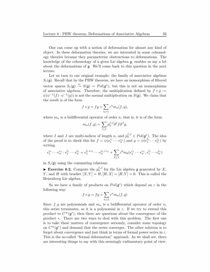
One can come up with a notion of deformation for almost any kind ofobject. In these deformation theories, we are interested in some cohomol-ogy theories because they parameterize obstructions to deformations. Theknowledge of the cohomology of a given Lie algebra g, enables us say a lotabout the deformations of g. We’ll come back to this question in the nextlecture.
Let us turn to our original example: the family of associative algebrasSε(g). Recall that by the PBW theorem, we have an isomorphism of filtered
vector spaces Sε(g)ψ→ S(g) = Pol(g∗), but this is not an isomorphisms
of associative algebras. Therefore, the multiplication defined by f ∗ g :=ψ(ψ−1(f) ·ψ−1(g)) is not the normal multiplication on S(g). We claim thatthe result is of the form
f ∗ g = fg +∑
n≥1
εnmn(f, g),
where mn is a bidifferential operator of order n, that is, it is of the form
mn(f, g) =∑
I,J
pI,Jn ∂If∂Jg,
where I and J are multi-indices of length n, and pI,Jn ∈ Pol(g∗). The ideaof the proof is to check this for f = ψ(er11 · · · ernn ) and g = ψ(el11 · · · elnn ) bywriting
er11 · · · ernn · el11 · · · elnn = el1+r11 · · · eln+rn
n +∑
k≥1
εkmk(er11 · · · ernn , el11 · · · elnn )
in Sε(g) using the commuting relations.
Exercise 8.2. Compute the pI,Jn for the Lie algebra g generated by X,Y , and H with bracket [X,Y ] = H, [H,X] = [H,Y ] = 0. This is called theHeisenberg Lie algebra.
So we have a family of products on Pol(g∗) which depend on ε in thefollowing way:
f ∗ g = fg +∑
n≥1
εnmn(f, g)
Since f, g are polynomials and mn is a bidifferential operator of order n,this series terminates, so it is a polynomial in ε. If we try to extend thisproduct to C∞(g∗), then there are questions about the convergence of theproduct ∗. There are two ways to deal with this problem. The first oneis to take these matters of convergence seriously, consider some topologyon C∞(g∗) and demand that the series converges. The other solution is toforget about convergence and just think in terms of formal power series in ε.This is the so-called “formal deformation” approach. As we shall see, thereare interesting things to say with this seemingly rudimentary point of view.

Lecture 8 - PBW theorem, Deformations of Associative Algebras 34
Formal deformations of associative algebras
Let (A,m0) be an associative algebra over C. Then, a formal deformationof (A,m0) is a C[[h]]-linear map m : A[[h]] ⊗C[[h]] A[[h]] → A[[h]] such that
m(a, b) = m0(a, b) +∑
n≥1
hnmn(a, b)
for all a, b ∈ A, and such that (A[[h]],m) is an associative algebra. Wesay that two formal deformations m and m are equivalent if there is aC[[h]]-automorphism A[[h]]
ϕ−→ A[[h]] such that m = mϕ, with ϕ(x) =x+
∑
n≥1 hnϕn(x) for all x ∈ A, where ϕn is an endomorphism of A.
Question: Describe the equivalence classes of formal deformations of a givenassociative algebra.
When (A,m0) is a commutative algebra, the answer is known. Philo-sophically and historically, this case is relevant to quantum mechanics. Inclassical mechanics, observables are smooth functions on a phase space M ,i.e they form a commutative associative algebra C∞(M). But when youquantize this system (which is needed to describe something on the orderof the Planck scale), you cannot think of observables as functions on phasespace anymore. You need to deform the commutative algebra C∞(M) to anoncommutative algebra. And it works...
From now on, let (A,m0) be a commutative associative algebra. Let’swrite m0(a, b) = ab, and m(a, b) = a ∗ b. (This is called a star product, andthe terminology goes back to the sixties and the work of J. Vey). Then wehave
a ∗ b = ab+∑
n≥1
hnmn(a, b).
Demanding the associativity of ∗ imposes an infinite number of equationsfor the mn’s, one for each order:
h0: a(bc) = (ab)c
h1: am1(b, c) +m1(a, bc) = m1(a, b)c+m1(ab, c)
h2: . . .
...
Exercise 8.3. Show that the bracket a, b = m1(a, b)−m1(b, a) defines aPoisson structure on A. This means that we can think of a Poisson structureon an algebra as the remnants of a deformed product where a ∗ b− b ∗ a =ha, b +O(h).
Lecture 8 - PBW theorem, Deformations of Associative Algebras 35
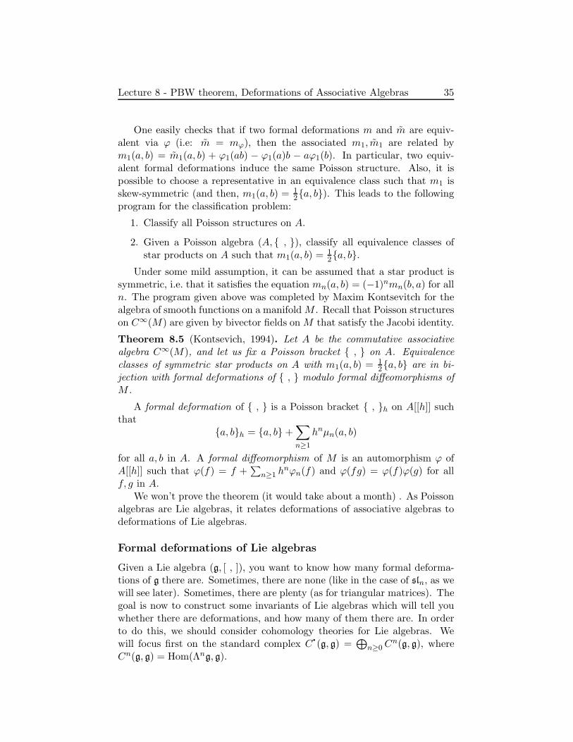
One easily checks that if two formal deformations m and m are equiv-alent via ϕ (i.e: m = mϕ), then the associated m1, m1 are related bym1(a, b) = m1(a, b) + ϕ1(ab) − ϕ1(a)b − aϕ1(b). In particular, two equiv-alent formal deformations induce the same Poisson structure. Also, it ispossible to choose a representative in an equivalence class such that m1 isskew-symmetric (and then, m1(a, b) = 1
2a, b). This leads to the followingprogram for the classification problem:
1. Classify all Poisson structures on A.
2. Given a Poisson algebra (A, , ), classify all equivalence classes ofstar products on A such that m1(a, b) = 1
2a, b.Under some mild assumption, it can be assumed that a star product is
symmetric, i.e. that it satisfies the equation mn(a, b) = (−1)nmn(b, a) for alln. The program given above was completed by Maxim Kontsevitch for thealgebra of smooth functions on a manifold M . Recall that Poisson structureson C∞(M) are given by bivector fields on M that satisfy the Jacobi identity.
Theorem 8.5 (Kontsevich, 1994). Let A be the commutative associativealgebra C∞(M), and let us fix a Poisson bracket , on A. Equivalenceclasses of symmetric star products on A with m1(a, b) = 1
2a, b are in bi-jection with formal deformations of , modulo formal diffeomorphisms ofM .
A formal deformation of , is a Poisson bracket , h on A[[h]] suchthat
a, bh = a, b +∑
n≥1
hnµn(a, b)
for all a, b in A. A formal diffeomorphism of M is an automorphism ϕ ofA[[h]] such that ϕ(f) = f +
∑
n≥1 hnϕn(f) and ϕ(fg) = ϕ(f)ϕ(g) for all
f, g in A.We won’t prove the theorem (it would take about a month) . As Poisson
algebras are Lie algebras, it relates deformations of associative algebras todeformations of Lie algebras.
Formal deformations of Lie algebras
Given a Lie algebra (g, [ , ]), you want to know how many formal deforma-tions of g there are. Sometimes, there are none (like in the case of sln, as wewill see later). Sometimes, there are plenty (as for triangular matrices). Thegoal is now to construct some invariants of Lie algebras which will tell youwhether there are deformations, and how many of them there are. In orderto do this, we should consider cohomology theories for Lie algebras. Wewill focus first on the standard complex C·(g, g) =
⊕
n≥0Cn(g, g), where
Cn(g, g) = Hom(Λng, g).
Lecture 9 36
Lecture 9
Let’s summarize what has happened in the last couple of lectures.
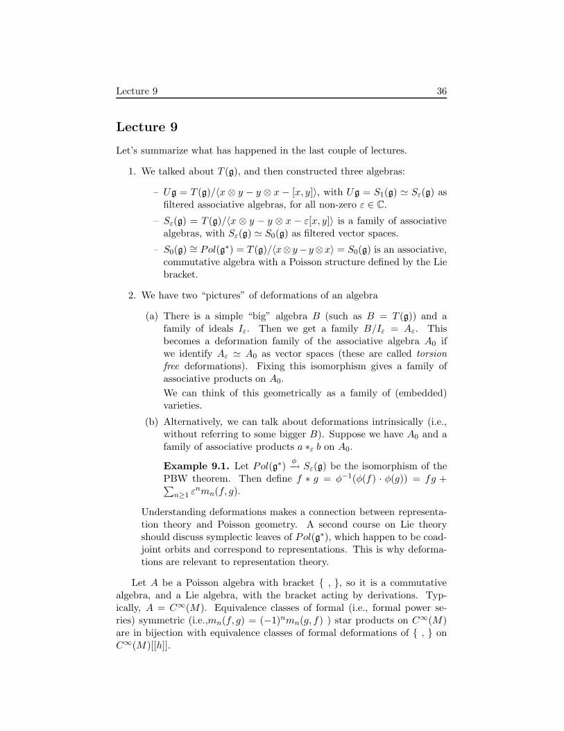
1. We talked about T (g), and then constructed three algebras:
– Ug = T (g)/〈x ⊗ y − y ⊗ x − [x, y]〉, with Ug = S1(g) ≃ Sε(g) asfiltered associative algebras, for all non-zero ε ∈ C.
– Sε(g) = T (g)/〈x ⊗ y − y ⊗ x − ε[x, y]〉 is a family of associativealgebras, with Sε(g) ≃ S0(g) as filtered vector spaces.
– S0(g) ∼= Pol(g∗) = T (g)/〈x⊗y−y⊗x〉 = S0(g) is an associative,commutative algebra with a Poisson structure defined by the Liebracket.
2. We have two “pictures” of deformations of an algebra
(a) There is a simple “big” algebra B (such as B = T (g)) and afamily of ideals Iε. Then we get a family B/Iε = Aε. Thisbecomes a deformation family of the associative algebra A0 ifwe identify Aε ≃ A0 as vector spaces (these are called torsionfree deformations). Fixing this isomorphism gives a family ofassociative products on A0.
We can think of this geometrically as a family of (embedded)varieties.
(b) Alternatively, we can talk about deformations intrinsically (i.e.,without referring to some bigger B). Suppose we have A0 and afamily of associative products a ∗ε b on A0.
Example 9.1. Let Pol(g∗)φ−→ Sε(g) be the isomorphism of the
PBW theorem. Then define f ∗ g = φ−1(φ(f) · φ(g)) = fg +∑
n≥1 εnmn(f, g).
Understanding deformations makes a connection between representa-tion theory and Poisson geometry. A second course on Lie theoryshould discuss symplectic leaves of Pol(g∗), which happen to be coad-joint orbits and correspond to representations. This is why deforma-tions are relevant to representation theory.
Let A be a Poisson algebra with bracket , , so it is a commutativealgebra, and a Lie algebra, with the bracket acting by derivations. Typ-ically, A = C∞(M). Equivalence classes of formal (i.e., formal power se-ries) symmetric (i.e.,mn(f, g) = (−1)nmn(g, f) ) star products on C∞(M)are in bijection with equivalence classes of formal deformations of , onC∞(M)[[h]].
Lecture 9 37
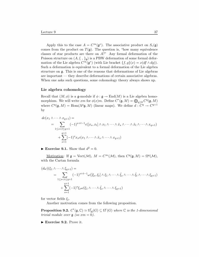
Apply this to the case A = C∞(g∗). The associative product on Sε(g)comes from the product on T (g). The question is, “how many equivalenceclasses of star products are there on A?” Any formal deformation of thePoisson structure on (A, , g) is a PBW deformation of some formal defor-mation of the Lie algebra C∞(g∗) (with Lie bracket f, g(x) = x(df ∧ dg)).Such a deformation is equivalent to a formal deformation of the Lie algebrastructure on g. This is one of the reasons that deformations of Lie algebrasare important — they describe deformations of certain associative algebras.When one asks such questions, some cohomology theory always shows up.
Lie algebra cohomology
Recall that (M,φ) is a g-module if φ : g → End(M) is a Lie algebra homo-morphism. We will write xm for φ(x)m. Define C·(g,M) =
⊕
q≥0 Cq(g,M)
where Cq(g,M) = Hom(Λqg,M) (linear maps). We define d : Cq → Cq+1
by
dc(x1 ∧ · · · ∧ xq+1) =
=∑
1≤s<t≤q+1
(−1)s+t−1c([xs, xt] ∧ x1 ∧ · · · ∧ xs ∧ · · · ∧ xt ∧ · · · ∧ xq+1)
+
q+1∑
s=1
(−1)sxsc(x1 ∧ · · · ∧ xs ∧ · · · ∧ xq+1)
Exercise 9.1. Show that d2 = 0.
Motivation: If g = Vect(M), M = C∞(M), then Cq(g,M) = Ωq(M),with the Cartan formula
(dω)(ξ1 ∧ · · · ∧ ξq+1) =
=∑
1≤s<t≤q+1
(−1)s+t−1ω([ξs, ξt] ∧ ξ1 ∧ · · · ∧ ξs ∧ · · · ∧ ξt ∧ · · · ∧ ξq+1)
+
q+1∑
s=1
(−1)sξsω(ξ1 ∧ · · · ∧ ξs ∧ · · · ∧ ξq+1)
for vector fields ξi.Another motivation comes from the following proposition.
Proposition 9.2. C·(g,C) ≃ Ω·R(G) ⊆ Ω·(G) where C is the 1-dimensionaltrivial module over g (so xm = 0).
Exercise 9.2. Prove it.

Lecture 9 38
Remark 9.3. This was Cartan’s original motivation for Lie algebra coho-mology. It turns out that the inclusion Ω·R(G) → Ω·(G) is a homotopyequivalence of complexes (i.e. the two complexes have the same homology),and the proposition above tells us that C·(g,C) is homotopy equivalent toΩR(G). Thus, by computing the Lie algebra cohomology of g (the homologyof the complex C·(g,C)), one obtains the De Rham cohomology of G (thehomology of the complex Ω·(G)).
Define Hq(g,M) = ker(d : Cq → Cq+1)/ im(d : Cq−1 → Cq) as always.Let’s focus on the case M = g, the adjoint representation: x ·m = [x,m].
H0(g, g) We have that C0 = Hom(C, g) ∼= g, and
dc(y) = y · c = [y, c].
so ker(d : C0 → C1) is the set of c ∈ g such that [y, c] = 0 for all y ∈ g.That is, the kernel is the center of g, Z(g). So H0(g, g) = Z(g).
H1(g, g) The kernel of d : C1(g, g) → C2(g, g) is
µ : g → g|dµ(x, y) = µ([x, y])−[x, µ(y)]−[µ(x), y] = 0 for all x, y ∈ g,
which is exactly the set of derivations of g. The image of d : C0(g, g) →C1(g, g) is the set of inner derivations, dc : g → g|dc(y) = [y, c]. TheLiebniz rule is satisfied because of the Jacobi identity. So
H1(g, g) = derivations/inner derivations =: outer derivations.
H2(g, g) Let’s compute H2(g, g). Suppose µ ∈ C2, so µ : g ∧ g → g is a linearmap. What does dµ = 0 mean?
dµ(x1, x2, x3) = µ([x1, x2], x3) − µ([x1, x3], x2) + µ([x2, x3], x1)
− [x1, µ(x2, x3)] + [x2, µ(x1, x3)] − [x3, µ(x1, x2)]
= −µ(x1, [x2, x3]) − [x1, µ(x2, x3)] + cyclic permutations
Where does this kind of thing show up naturally?
Consider deformations of Lie algebras:
[x, y]h = [x, y] +∑
n≥1
hnmn(x, y)
where the mn : g × g → g are bilinear. The deformed bracket [ , ]hmust satisfy the Jacobi identity,
[a, [b, c]h]h + [b, [c, a]h]h + [c, [a, b]h]h = 0
Lecture 9 39
which gives us relations on the mn. In degree hN , we get
[a,mN (b, c)] +mN (a, [b, c]) +
N−1∑
k=1
mk(a,mN−k(b, c))+
[b,mN (c, a)] +mN (b, [c, a]) +N−1∑
k=1
mk(b,mN−k(c, a))+
[c,mN (a, b)] +mN (c, [a, b]) +
N−1∑
k=1
mk(c,mN−k(a, b)) = 0 (†)
Exercise 9.3. Derive (†).
Define [mK ,mN−K ](a, b, c) as
mK
(a,mN−K(b, c)
)+mK
(b,mN−K(c, a)
)+mK
(c,mN−K(a, b)
).
Then (†) can be written as
dmN =
N−1∑
k=1
[mk,mN−k] (‡)
Theorem 9.4. Assume that for all n ≤ N − 1, we have the relationdmn =
∑n−1k=1 [mk,mn−k]. Then d(
∑N−1k=1 [mk,mN−k]) = 0.
Exercise 9.4. Prove it.
The theorem tells us that if we have a “partial deformation” (i.e. wehave found m1, . . . ,mN−1), then the expression
∑N−1k=1 [mk,mN−k] is
a 3-cocycle. Furthermore, (‡) tells us that if we are to extend ourdeformation to one higher order,
∑N−1k=1 [mk,mN−k] must represent
zero in H3(g, g).
Taking N = 1, we get dm1 = 0, so ker(d : C2 → C3) = space of firstcoefficients of formal deformations of [ , ]. It will turn out that H2 isthe space of equivalence classes of m1.
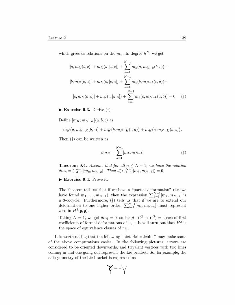
It is worth noting that the following “pictorial calculus” may make someof the above computations easier. In the following pictures, arrows areconsidered to be oriented downwards, and trivalent vertices with two linescoming in and one going out represent the Lie bracket. So, for example, theantisymmetry of the Lie bracket is expressed as
= − ////
Lecture 9 40
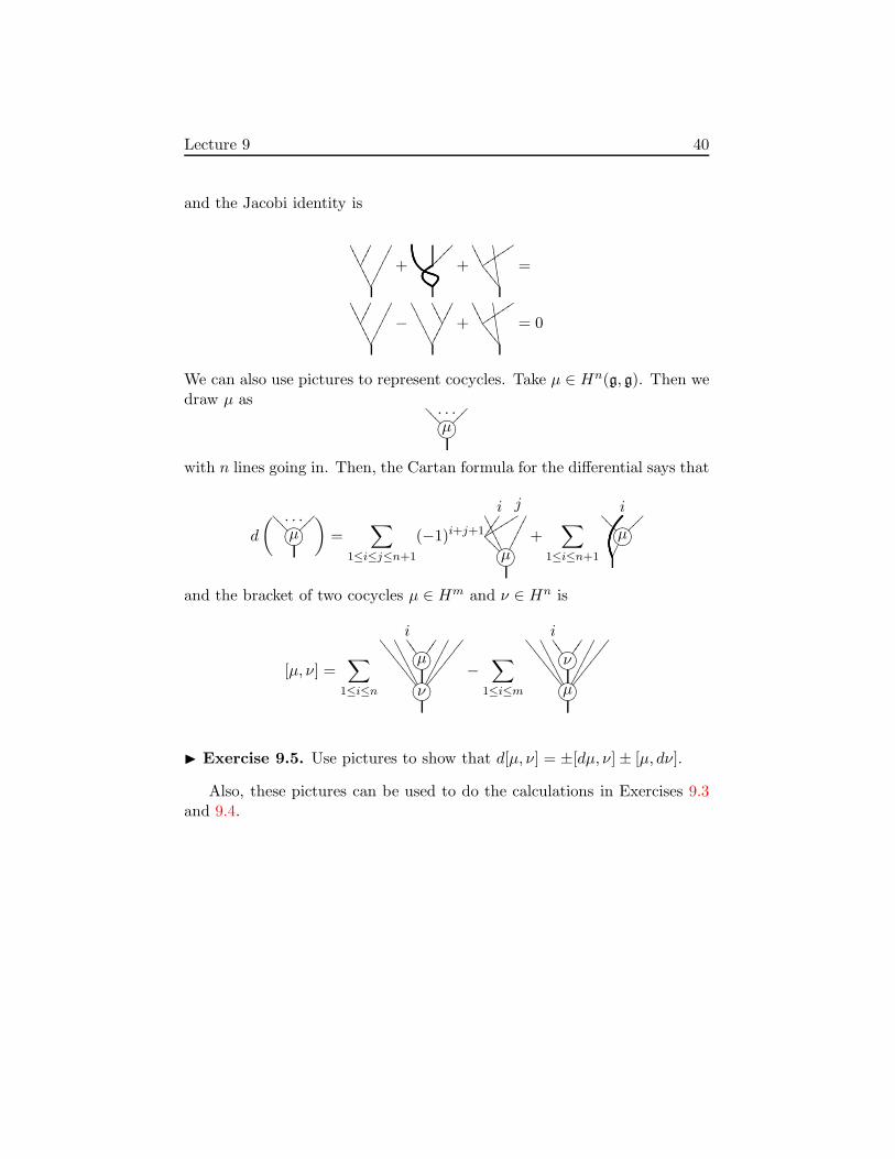
and the Jacobi identity is
////
////
+
+//
//
$$$$$$
tttttt
9999 =
////
////
−//
////
///
//
+//
//
$$$$$$
tttttt
9999 = 0
We can also use pictures to represent cocycles. Take µ ∈ Hn(g, g). Then wedraw µ as
µ(/).*-+,??? . . .
with n lines going in. Then, the Cartan formula for the differential says that
d
(
µ(/).*-+,??? . . . )
=∑
1≤i≤j≤n+1
(−1)i+j+1
i
j
sssss
s
µ(/).*-+,???
//////
+
∑
1≤i≤n+1
µ(/).*-+,???
i
and the bracket of two cocycles µ ∈ Hm and ν ∈ Hn is
[µ, ν] =∑
1≤i≤n
µ(/).*-+,i555
ν(/).*-+,
99999999
0000000
−∑
1≤i≤m
ν(/).*-+,i555
µ(/).*-+,
99999999
0000000
Exercise 9.5. Use pictures to show that d[µ, ν] = ±[dµ, ν] ± [µ, dν].
Also, these pictures can be used to do the calculations in Exercises 9.3and 9.4.
Lecture 10 41
Lecture 10
Here is the take-home exam, it’s due on Tuesday:
(1) B ⊂ SL2(C) are upper triangular matrices, then
– Describe X = SL2(C)/B
– SL2(C) acts on itself via left multiplication implies that it actson X. Describe the action.
(2) Find exp
0 x1 0. . .
. . .
0 xn−1
0 0
(3) Prove that if V,W are filtered vector spaces (with increasing filtration)and φ : V → W satisfies φ(Vi) ⊆ Wi, and Gr(φ) : Gr(V )
∼−→ Gr(W )an isomorphism, then φ is a linear isomorphism of filtered spaces.
Lie algebra cohomology
Recall C·(g,M) from the previous lecture, for M a finite dimensional rep-resentation of g (and g finite dimensional). There is a book by D. Fuchs,Cohomology of ∞-dimensional Lie algebras [Fuc50].
We computed that H0(g, g) = Z(g) ≃ g/[g, g] and that H1(g, g) is thespace of exterior derivations of g. Say c ∈ Z1(g, g),1 so [c] ∈ H1(g, g). Definegc = g⊕C∂c with the bracket [(x, t), (y, s)] = ([x, y]− tc(y)+ sc(x), 0). So ife1, . . . , en is a basis in g with the usual relations [ei, ej ] = ckijek, then we get
one more generator ∂c such that [∂c, x] = c(x). Then H1(g, g) is the spaceof equivalence classes of extensions
0 → g → g → C→ 0
up to the equivalences f such that the diagram commutes:
0 // g //
Id
g //
f
C
Id
// 0
0 // g // g′ // C // 0
This is the same as the space of exterior derivations.
1Zn(g,M) is the space of n-cocycles, i.e. the kernel of d : Cn(g, M) → Cn+1(g, M).

Lecture 10 42
H2(g, g) and Deformations of Lie algebras
A deformation of g is the vector space g[[h]] with a bracket [a, b]h = [a, b] +∑
n≥1 hnmn(a, b) such that mn(a, b) = −mn(b, a) and
[a, [b, c]h]h + [b, [c, a]h]h + [c, [a, b]h]h = 0.
The hN order term of the Jacobi identity is the condition
[a,mN (b, c)] +mN (a, [b, c]) +
N−1∑
k=1
mk(a,mN−k(b, c)) + cycle = 0 (††)
For µ ∈ C2(g, g), we compute
dµ(a, b, c) = −[a, µ(b, c)] − µ(a, [b, c]) + cycle.
Definemk,mN−k(a, b, c)
def= mk(a,mN−k(b, c)) + cycle
This is called the Gerstenhaber bracket ... do a Google search for it if youlike ... it is a tiny definition from a great big theory.
Then we can rewrite (††) as
dmN =
N−1∑
k=1
mk,mN−k. (‡)
In partiular, dm1 = 0, so m1 is in Z2(g, g).Equivalences: [a, b]′h ≃ [a, b]h if [a, b]′h = φ−1([φ(a), φ(b)]h) for some
φ(a) = a+∑
n≥1 hnφn(a). then
m′1(a, b) = m1(a, b) − φ1([a, b]) + [a, φ1(b)] + [φ1(a), b].
which we can write as m′1 = m1 + dφ1. From this we can conclude
Claim. The space of equivalence classes of possible m1 is exactly H2(g, g).
Claim (was HW). If m1 is a 2-cocycle, and mN−1, . . . ,m2 satisfy the equa-tions we want, then
d
(N−1∑
k=1
mk,mN−k)
= 0.
This is not enough; we know that∑N+1
k=1 mk,mN−k is in Z3(g, g), butto find mN , we need it to be trivial in H3(g, g) because of (‡). If thecohomology class of
∑N+1k=1 mk,mN−k is non-zero, it’s class in H3(g, g) is
called an obstruction to n-th order deformation. If H3(g, g) is zero, then any
Lecture 10 43
first order deformation (element of H2(g, g)) extends to a deformation, but ifH3(g, g) is non-zero, then we don’t know that we can always extend. Thus,H3(g, g) is the space of all possible obstructions to extending a deformation.
Let’s keep looking at cohomology spaces. Consider C·(g,C), where C isa one dimensional trivial representation of g given by x 7→ 0 for any x ∈ g.
First question: take Ug, with the corresponding 1-dimensional represen-tation ε : Ug → C given by ε(x) = 0 for x ∈ g.
Exercise 10.1. Show that (Ug, ε,∆, S) is a Hopf algebra with the εabove, ∆(x) = 1 ⊗ x+ x⊗ 1, and S(x) = −x for x ∈ g. Remember that ∆and ε are algebra homomorphisms, and that S is an anti-homomorphism.
Let’s compute H1(g,C) (H0 is boring, just a point). This is ker(C1 d−→C2). Well, C1(g,C) = Hom(g,C), C2(g,C) = Hom(Λ2g,C), and
dc(x, y) = c([x, y]).
So the kernel is the set of c such that c([x, y]) = 0 for all x, y ∈ g. Thus,ker(d) ⊆ C1(g,C) is the space of g-invariant linear functionals. Recall thatg acts on g by the adjoint action, and on g∗ = C1(g, g) by the coadjointaction (x : l 7→ lx where lx(y) = l([x, y])). Under the coadjoint action, l ∈ g∗
is g-invariant if lx = 0. Note that C0 is just one point, so its image doesn’thave anything in it.
Now let’s compute H2(g,C) = ker(d : C2 → C3)/ im(d : C1 → C2). Letc ∈ Z2, then
dc(x, y, z) = c([x, y], z) − c([x, z], y) + c([y, z], x) = 0
for all x, y, z ∈ g. Now let’s find the image of d : C1 → C2: it is the set offunctions of the form dl(x, y) = l([x, y]) where l ∈ g∗. It is clear that l([x, y])are (trivial) 2-cocycles because of the Jacobi identity. Let’s see what can wecook with this H2.
Definition 10.1. A central extension of g is a short exact sequence
0 → C→ g → g → 0.
Two such extensions are equivalent if there is a Lie algebra isomorphismf : g → g′ such that the diagram commutes:
0 // C //
Id
g //
f
g
Id
// 0
0 // C // g′ // g // 0
Lecture 10 44
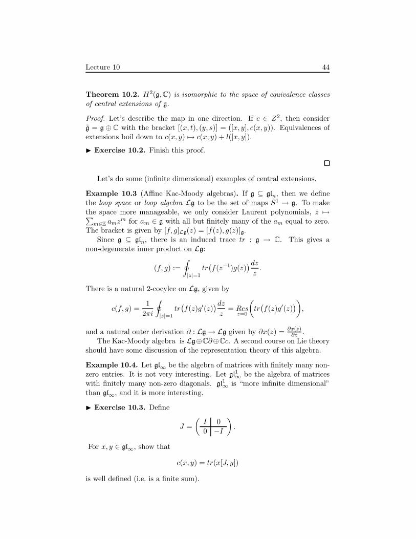
Theorem 10.2. H2(g,C) is isomorphic to the space of equivalence classesof central extensions of g.
Proof. Let’s describe the map in one direction. If c ∈ Z2, then considerg = g ⊕ C with the bracket [(x, t), (y, s)] = ([x, y], c(x, y)). Equivalences ofextensions boil down to c(x, y) 7→ c(x, y) + l([x, y]).
Exercise 10.2. Finish this proof.
Let’s do some (infinite dimensional) examples of central extensions.
Example 10.3 (Affine Kac-Moody algebras). If g ⊆ gln, then we definethe loop space or loop algebra Lg to be the set of maps S1 → g. To makethe space more manageable, we only consider Laurent polynomials, z 7→∑
m∈Zamz
m for am ∈ g with all but finitely many of the am equal to zero.The bracket is given by [f, g]Lg(z) = [f(z), g(z)]g.
Since g ⊆ gln, there is an induced trace tr : g → C. This gives anon-degenerate inner product on Lg:
(f, g) :=
∮
|z|=1tr(f(z−1)g(z)
)dz
z.
There is a natural 2-cocylce on Lg, given by
c(f, g) =1
2πi
∮
|z|=1tr(f(z)g′(z)
)dz
z= Res
z=0
(
tr(f(z)g′(z)
))
,
and a natural outer derivation ∂ : Lg → Lg given by ∂x(z) = ∂x(z)∂z .
The Kac-Moody algebra is Lg⊕C∂⊕Cc. A second course on Lie theoryshould have some discussion of the representation theory of this algebra.
Example 10.4. Let gl∞ be the algebra of matrices with finitely many non-zero entries. It is not very interesting. Let gl1∞ be the algebra of matriceswith finitely many non-zero diagonals. gl1∞ is “more infinite dimensional”than gl∞, and it is more interesting.
Exercise 10.3. Define
J =
(I 0
0 −I
)
.
For x, y ∈ gl∞, show that
c(x, y) = tr(x[J, y])
is well defined (i.e. is a finite sum).

Lecture 10 45
This c is a non-trivial 1-cocycle, i.e. [c] ∈ H2(gl1∞,C) is non-zero. By theway, instead of just using linear maps, we require that the maps Λ2gl1∞ → Care graded linear maps. This is H2
graded.Notice that in gln, tr(x[J, y]) = tr(J [x, y]) is a trivial cocycle (it is d of
l(x) = tr(Jx). So we have that H2(gln,C) = 0.We can define a∞ = gl∞⊕Cc. This is some non-trivial central extension.
To summarize the last lectures:
1. We related Lie algebras and Lie Groups. If you’re interested in repre-sentations of Lie Groups, looking at Lie algebras is easier.
2. From a Lie algebra g, we constructed Ug, the universal envelopingalgebra. This got us thinking about associative algebras and Hopfalgebras.
3. We learned about dual pairings of Hopf algebras. For example, C[Γ]and C(Γ) are dual, and Ug and C(G) are dual (if G is affine alge-braic and we are looking at polynomial functions). This pairing is astarting point for many geometric realizations of representations of G.Conceptually, the notion of the universal enveloping algebra is closelyrelated to the notion of the group algebra C[Γ].
4. Finally, we talked about deformations.
Lecture 11 - Engel’s Theorem and Lie’s Theorem 46
Lecture 11 - Engel’s Theorem and Lie’s Theorem
The new lecturer is Vera Serganova.We will cover
1. Classification of semisimple Lie algebras. This will include root sys-tems and Dynkin diagrams.
2. (1) will lead to a classification of compact connected Lie Groups.
3. Finally, we will talk about representation theory of semisimple Liealgebras and the Weyl character formula.
A reference for this material is Fulton and Harris [FH91].The first part is purely algebraic: we will study Lie algebras. g will be a
lie algebra, usually finite dimensional, over a field k (usually of characteristic0).
Any Lie algebra g contains the ideal D(g) = [g, g], the vector subspacegenerated by elements of the form [X,Y ] for X,Y ∈ g.
Exercise 11.1. Show that Dg is an ideal in g.
Exercise 11.2. Let G be a simply connected Lie group with Lie algebrag. Then [G,G] is the subgroup of G generated by elements of the formghg−1h−1 for g, h ∈ G. Show that [G,G] is a connected closed normal Liesubgroup of G, with Lie algebra Dg.
Warning 11.1. Exercise 11.2 is a tricky problem. Here are some poten-tial pitfalls:
1. For G connected, we do not necessarily know that the exponentialmap is surjective, because G may not be complete. For example,exp : sl2(C) → SL2(C) is not surjective.1
2. If H ⊆ G is a subgroup with Lie algebra h, then h ⊆ g closed is notenough to know that H is closed in G. For example, take G to be atorus, and H to be a line with irrational slope.
3. This exercise requires G to be simply connected. Let
H :==
1 x y0 1 z0 0 1
× S1
K :=
(0 1 0 n0 1 00 0 1
1A, cn) ∣∣∣∣n ∈ Z
⊆ H
1Assume−1 10 −1
is in the image, then its pre-image must have eigenvalues (2n + 1)iπ
and −(2n + 1)iπ for some integer n. So the pre-image has distinct eigenvalues, so it isdiagonalizable. But that implies that
−1 10 −1
is diagonalizable, contradiction.
Lecture 11 - Engel’s Theorem and Lie’s Theorem 47
where c is an element of S1 of infinite order. Then K is normal in Hand G = H/K is a counterexample.
Definition 11.2. Define D0g = g, and Dng = [Dn−1g,Dn−1g]. This iscalled the derived series of g. We say g is solvable if Dng = 0 for some nsufficiently large.
Definition 11.3. We can also define D0g = g, and Dng = [g,Dn−1g]. Thisis called the lower central series of g. We say that g is nilpotent if Dng = 0for some n sufficiently large.
We will denote D1g = D1g by Dg. Solvable and nilpotent lie algebrasare hard to classify. Instead, we will do the classification of semisimple Liealgebras (see Definition 11.15).
The following example is in some sense universal (see corollaries 11.7 and11.12):
Example 11.4. Let gl(n) be the Lie algebra of all n × n matrices, and letb be the subalgebra of upper triangular matrices. I claim that b is solvable.To see this, note that Db is the algebra of strictly upper triangular matrices,and in general, Dkb has zeros on the main diagonal and the 2k−2 diagonalsabove the main diagonal (for k ≥ 2). Let n = Db. You can check that n isin fact nilpotent.
Useful facts about solvable/nilpotent Lie algebras:
1. If you have an exact sequence of Lie algebras
0 → a → g → g/a → 0
then g is solvable if and only if a and g/a are solvable.
2. If you have an exact sequence of Lie algebras
0 → a → g → g/a → 0
then if g is nilpotent, so are a and g/a.
Warning 11.5. The converse is not true. Diagonal matrices d is nilpo-tent, and we have
0 → n → b → d → 0.
Note that b is not nilpotent, because Db = Dnb =(
0 ∗0 0
).

Lecture 11 - Engel’s Theorem and Lie’s Theorem 48
3. If a, b ⊂ g are solvable ideals, then the sum a + b is solvable. To seethis, note that we have
0 → a → a + b → (a + b)/a︸ ︷︷ ︸
≃b/(a∩b)
→ 0
a is solvable by assumption, and b/(a ∩ b) is a quotient of a solvablealgebra, so it is solvable by (1). Applying (1) again, a + b is solvable.
4. If k ⊆ F is a field extension, with a Lie algebra g over k, we can makea lie algebra g ⊗k F over F . Note that g ⊗k F is solvable (nilpotent)if and only if g is.
We will now prove Engel’s theorem and Lie’s theorem.For any Lie algebra g, we have the adjoint representation: X 7→ adX ∈
gl(g) given by adX(Y ) = [X,Y ]. If g is nilpotent, then adX is a nilpotentoperator for any X ∈ g. The converse is also true as we will see shortly(Cor. 11.9).
Theorem 11.6 (Engel’s Theorem). Let g ⊆ gl(V ), and assume that X isnilpotent for any X ∈ g. Then there is a vector v ∈ V such that g · v = 0.
Note that the theorem holds for any representation ρ of g in which everyelement acts nilpotently; just replace g in the statement of the theorem byρ(g).
Corollary 11.7. If V is a representation of g in which every element actsnilpotently, then one can find 0 = V0 ( V1 ( · · · ( Vn = V a complete flagsuch that g(Vi) ⊆ Vi−1. That is, there is a basis in which all of the elementsof g are strictly upper triangular.
Warning 11.8. Note that the theorem isn’t true if you say “suppose g isnilpotent” instead of the right thing. For example, the set of diagonal
matrices d ⊂ gl(V ) is nilpotent.
Proof. Let’s prove the theorem by induction on dim g.We first show thatg has an ideal a of codimension 1. To see this, take a maximal propersubalgebra a ⊂ g. Look at the representation of a on the quotient space g/a.This representation, a → gl(g/a), satisfies the condition of the theorem,2 soby induction, there is some X ∈ g such that ada(X) = 0 modulo a. So[a,X] ⊆ a, so b = kX ⊕ a is a new subalgebra of g which is larger, so itmust be all of g. Thus, a must have had codimension 1. Therefore, a ⊆ g isactually an ideal (because [X, a] = 0).
2For any X ∈ a, since X is nilpotent, adX is also nilpotent.

Lecture 11 - Engel’s Theorem and Lie’s Theorem 49
Next, we prove the theorem. Let V0 = v ∈ V |av = 0, which is non-zero by the inductive hypothesis. We claim that gV0 ⊆ V0. To see this, takex ∈ g, v ∈ V0, and y ∈ a. We have to check that y(xv) = 0. But
yxv = x yv︸︷︷︸
0
+ [y, x]︸ ︷︷ ︸
∈a
v = 0.
Now, we have that g = kX ⊕ a, and a kills V0, and that X : V0 → V0 isnilpotent, so it has a kernel. Thus, there is some v ∈ V0 which is killed byX, and so v is killed by all of g.
Corollary 11.9. If adX is nilpotent for every X ∈ g, then g is nilpotent asa Lie algebra.
Proof. Let V = g, so we have ad : g → gl(g), which has kernel Z(g). ByEngel’s theorem, we know that there is an x ∈ g such that (ad g)(x) = 0.This implies that Z(g) 6= 0. By induction we can assume g/Z(g) is nilpotent.But then g itself must be nilpotent as well because Dn(g/Z(g)) = 0 impliesDn+1(g) = 0.
Warning 11.10. If g ⊆ gl(V ) is a nilpotent subalgebra, it does not implythat every X ∈ g is nilpotent (take diagonal matrices for example).
Theorem 11.11 (Lie’s Theorem). Let k be algebraically closed and of char-acteristic 0. If g ⊆ gl(V ) is a solvable subalgebra, then all elements of g havea common eigenvector in V .
This is a generalization of the statement that two commuting operators havea common eigenvector.
Corollary 11.12. If g is solvable, then there is a complete flag 0 = V0 V1 · · · Vn = V such that g(Vi) ⊆ Vi. That is, there is a basis in whichall elements of g are upper triangular.
Proof. If g is solvable, take any subspace a ⊂ g of codimension 1 containingDg, then a is an ideal. We’re going to try to do the same kind of inductionas in Engel’s theorem.
For a linear functional λ : a → k, let
Vλ = v ∈ V |Xv = λ(X)v for all X ∈ a.
Vλ 6= 0 for some λ by induction hypothesis.
Claim. g(Vλ) ⊆ Vλ.
Lecture 11 - Engel’s Theorem and Lie’s Theorem 50
Proof of Claim. Choose v ∈ Vλ and X ∈ a, Y ∈ g. Then
X(Y v) = Y ( Xv︸︷︷︸
λ(X)v
) + [X,Y ]v︸ ︷︷ ︸
λ([X,Y ])v
We want to show that λ[X,Y ] = 0. There is a trick. Let r be the largestinteger such that v, Y v, Y 2v, . . . , Y rv is a linearly independent set. Weknow that Xv = λ(X)v for any X ∈ a. We claim that XY jv ≡ λ(X)Y jvmod (spanv, Y v, . . . , Y j−1v). This is clear for j = 0, and by induction,we have
XY jv = YXY j−1v︸ ︷︷ ︸
≡λ(X)Y j−1vmod spanv,...,Y j−2v
+ [X,Y ]Y j−1v︸ ︷︷ ︸
≡λ([X,Y ])Y j−1vmod spanv,...,Y j−2v
≡ λ(X)Y jv mod spanv, . . . , Y j−1v
So the matrix for X can be written as λ(X) on the diagonal and stuffabove the diagonal (in this basis). So the trace of X is (r + 1)λ(X). Thenwe have that tr([X,Y ]) = (r + 1)λ([X,Y ]), since the above statement wasproved for any X ∈ a and [X,Y ] ∈ a. But the trace of a commutator isalways 0. Since the characteristic of k is 0, we can conclude that λ[X,Y ] = 0.
Claim
To finish the proof, write g = kT ⊕ a, with T : Vλ → Vλ (we can dothis because of the claim). Since k is algebraically closed, T has a non-zeroeigenvector w in Vλ. This w is the desired common eigenvector.
Remark 11.13. If k is not algebraically closed, the theorem doesn’t hold. Forexample, consider the (one-dimensional) Lie algebra generated by a rotationof R2.
The theorem also fails if k is not characteristic 0. Say k is characteristicp, then let x be the permutation matrix of the p-cycle (p p− 1 · · · 2 1) (i.e.the matrix
(0 Ip−1
1 0
)), and let y be the diagonal matrix diag(0, 1, 2, . . . , p−1).
Then [x, y] = x, so the Lie algebra generated by x and y is solvable. However,y is diagonal, so we know all of its eigenvectors, and none of them is aneigenvector of x.
Corollary 11.14. Let k be of characteristic 0. Then g is solvable if andonly if Dg is nilpotent.
If Dg is nilpotent, then g is solvable from the definitions. If g is solvable,then look at everything over the algebraic closure of k, where g looks likeupper triangular matrices, so Dg is nilpotent. All this is independent ofcoefficients (by useful fact (4)).
Lecture 11 - Engel’s Theorem and Lie’s Theorem 51
The radical
There is a unique maximal solvable ideal in g (by useful fact (3): sum ofsolvable ideals is solvable), which is called the radical of g.
Definition 11.15. We call g semisimple if rad g = 0.
Exercise 11.3. Show that g/rad g is always semisimple.
If g is one dimensional, generated by X, then we have that [g, g] = 0, sog cannot be semisimple.
If g is two dimensional, generated by X and Y , then we have that [g, g] isone dimensional, spanned by [X,Y ]. Thus, g cannot be semisimple becauseDg is a solvable ideal.
There is a semisimple Lie algebra of dimension 3, namely sl2.Semisimple algebras have really nice properties. Cartan’s criterion (The-
orem 12.7) says that g is semisimple if and only if the Killing form (see nextlecture) is non-degenerate. Whitehead’s theorem (Theorem 12.10) says thatif V is a non-trivial irreducible representation of a semisimple Lie algebra g,then H i(g, V ) = 0 for all i. Weyl’s theorem (Theorem 12.14) says that ev-ery finite-dimensional representation of a semisimple Lie algebra is the directsum of irreducible representations. If G is simply connected and compact,the g is semisimple .

Lecture 12 - Cartan Criterion, Whitehead and Weyl Theorems 52
Lecture 12 - Cartan Criterion, Whitehead and Weyl
Theorems
Invariant forms and the Killing form
Let ρ : g → gl(V ) be a representation. To make the notation cleaner, wewill write X for ρ(X). We can define a bilinear form on g by BV (X,Y ) :=tr(XY ). This form is symmetric because tr(AB) = tr(BA) for any linearoperators A and B.
We also have that
BV ([X,Y ], Z) = tr(XY Z − Y XZ) = tr(XY Z) − tr(XZY )
= tr(XY Z − XZY ) = BV (X, [Y,Z]),
so B satisfiesB([X,Y ], Z) = B(X, [Y,Z]).
Such a form is called an invariant form. It is called invariant because it isimplied by B being Ad-invariant. Assume that for any g ∈ G and X,Z ∈ g,we B(AdgX,AdgZ) = B(X,Z). Let γ be a path in G with γ′(0) = Y . Weget that
B([Y,X], Z) +B(X, [Y,Z]) =d
dt
∣∣∣∣t=0
B(Adγ(t)(X), Adγ(t)(Z)
)= 0.
Definition 12.1. The Killing form, denoted by B, is the special case whereρ is the adjoint representation. That is, B(X,Y ) := tr(adX adY ).
Exercise 12.1. Let g be a simple Lie algebra over an algebraically closedfield. Check that two invariant forms on g are proportional.
Exercise 12.2 (In class). If g is solvable, then B(g,Dg) = 0.
Solution. First note that if Z = [X,Y ] ∈ Dg, then adZ = [adX , adY ] ∈D(ad g) since the adjoint representation is a Lie algebra homomorphism.Moreover, g solvable implies the image of the adjoint representation, ad(g) ≃g/Z(g), is solvable. Therefore, in some basis of V of a representation ofad(g), all matrices of ad(g) are upper triangular (by Lie’s Theorem), andthose of D(adg) are all strictly upper triangular. The product of an uppertriangular matrix and a strictly upper triangular matrix will be strictlyupper triangular and therefore have trace 0.
The converse of this exercise is also true. It will follow as a corollary ofour next theorem (Corollary 12.6 below).
Theorem 12.2. Suppose g ⊆ gl(V ), char k = 0, and BV (g, g) = 0. Then g
is solvable.
Lecture 12 - Cartan Criterion, Whitehead and Weyl Theorems 53
For the proof, we will need the following facts from linear algebra.
Lemma 12.3.1 Let X be a diagonalizable linear operator in V , with k alge-braically closed. If X = A·diag(λ1, . . . , λn)·A−1 and f : k → k is a function,we define f(X) as A ·diag(f(λ1), . . . , f(λn)) ·A−1. Suppose tr(X ·f(X)) = 0for any Q-linear map f : k → k such that f is the identity on Q, then X = 0.
Proof. Consider only f such that the image of f is Q. Let λ1, . . . , λm be theeigenvalues of X with multiplicities n1, . . . , nm. We obtain tr(X · f(X)) =n1λ1f(λ1) + . . . + nmλmf(λn) = 0. Apply f to this identity to obtainn1f(λ1)
2 + . . .+nmf(λm)2 = 0 which implies f(λi) = 0 for all i. If some λiis not zero, we can choose f so that f(λi) 6= 0, so λi = 0 for all i. Since Xis diagonalizable, X = 0.
Lemma 12.4 (Jordan Decomposition). Given X ∈ gl(V ), there are uniqueXs,Xn ∈ gl(V ) such that Xs is diagonalizable, Xn is nilpotent, [Xs,Xn] = 0,and X = Xn +Xs. Furthermore, Xs and Xn are polynomials in X.
Proof. All but the last statement is standard; see, for example, Corollay 2.5of Chapter XIV of [Lan02]. To see the last statement, let the characteristicpolynomial of X be
∏
i(x−λi)ni . By the chinese remainder theorem, we canfind a polynomial f such that f(x) ≡ λi mod (x − λi)
ni . Choose a basisso that X is in Jordan form and compute f(X) block by block. On a blockwith λi along the diagonal (X − λiI)
ni is 0, so f(X) is λiI on this block.Then f(X) = Xs is diagonalizable and Xn = X − f(X) is nilpotent.
Lemma 12.5. Let g ⊆ gl(V ). The adjoint representation ad : g → gl(g)preserves Jordan decomposition: adXs = (adX)s and adXn = (adX)n. Inparticular, adXs is a polynomial in adX .
Proof. Suppose the eigenvalues of Xs are λ1, . . . , λm, and we are in a basiswhere Xs is diagonal. Check that adXs(Eij) = [Xs, Eij ] = (λi − λj)Eij . SoXs diagonalizable implies adXs is diagonalizable (because it has a basis ofeigenvectors). We have that adXn is nilpotent because the monomials in theexpansion of (adXn)k(Y ) have Xn to at least the k/2 power on one side of Y .So we have that adX = adXs + adXn , with adXs diagonalizable, adXn nilpo-tent, and the two commute, so by uniqueness of the Jordan decomposition,adXs = (adX)s and adXn = (adX)n.
Proof of Theorem 12.2. It is enough to show that Dg is nilpotent. Let X ∈Dg, so X =
∑[Yi, Zi]. It suffices to show that Xs = 0. To do this, let
1This is different from what we did in class. There is an easier way to do this if youare willing to assume k = C and use complex conjugation. See Fulton and Harris for thismethod.

Lecture 12 - Cartan Criterion, Whitehead and Weyl Theorems 54
f : k → k be any Q-linear map fixing Q.
BV (f(Xs),Xs) = BV (f(Xs),X) (Xn doesn’t contribute)
= BV
(
f(Xs),∑
i
[Yi, Zi])
=∑
i
BV ([f(Xs), Yi]︸ ︷︷ ︸
∈g?
, Zi) (BV invariant)
= 0 (assuming [f(Xs), Yi] ∈ g)
Then by Lemma 12.3, Xs = 0.To see that [f(Xs), Yi] ∈ g, suppose the eigenvalues of Xs are λ1, . . . , λm.
Then the eigenvalues of f(Xs) are f(λi), the eigenvalues of adXs are of theform µij := λi − λj, and eigenvalues of adf(Xs) are νij := f(λi) − f(λj) =f(µij). If we define g to be a polynomial such that g(µij) = νij, then adf(Xs)
and g(adXs) are diagonal (in some basis) with the same eigenvalues in thesame places, so they are equal. So we have
[f(Xs), Yi] = g(adXs)(Yi)
= h(adX)(Yi) ∈ g (using Lemma 12.5)
for some polynomial h.The above arguments assume k is algebraically closed, so if it’s not apply
the above to g ⊗k k. Then g ⊗k k solvable implies g solvable as mentionedin the previous lecture.
Corollary 12.6. g is solvable if and only if B(Dg, g) = 0.
Proof. (⇐) We have that B(Dg, g) = 0 implies B(Dg,Dg) = 0 which impliesthat ad(Dg) is solvable. The adjoint representation of Dg gives the exactsequence
0 → Z(Dg) → Dg → ad(Dg) → 0.
Since Z(Dg) and ad(Dg) are solvable, Dg is solvable by useful fact (1) ofLecture 11, so g is solvable.
(⇒) This is exercise 12.2.
Theorem 12.7 (Cartan’s Criterion). The Killing form is non-degenerate ifand only if g is semi-simple.
Proof. Say g is semisimple. Let a = kerB. Because B is invariant, we getthat a is an ideal, and B|a = 0. By the previous theorem (12.2), we havethat a is solvable, so a = 0 (by definition of semisimple).
Suppose that g is not semisimple, so g has a non-trivial solvable ideal.Then the last non-zero term in its upper central series is some abelian ideal

Lecture 12 - Cartan Criterion, Whitehead and Weyl Theorems 55
a ⊆ g2. For any X ∈ a, the matrix of adX is of the form(
0 ∗0 0
)with respect
to the decomposition g = a ⊕ g/a, and for Y ∈ g, adY is of the form( ∗ ∗
0 ∗).
Thus, we have that tr(adX adY ) = 0 so X ∈ kerB, so B is degenerate.
Theorem 12.8. Any semisimple Lie algebra is a direct sum of simple alge-bras.
Proof. If g is simple, then we are done. Otherwise, let a ⊆ g be an ideal,then the restriction B|a is nondegenerate. Note that a⊥ is also an ideal byinvariance of B. Look at a ∩ a⊥. On their intersection, B is zero, so theintersection is a solvable ideal, so it is zero. Thus, we have that g = a⊕ a⊥.By induction on dimension, we’re done.
Remark 12.9. In particular, if g =⊕
gi is semisimple, with each gi simple,we have that Dg =
⊕Dgi. But Dgi is either 0 or gi, and it cannot be 0(lest gi be a solvable ideal). Thus Dg = g.
Theorem 12.10 (Whitehead). If g is semisimple and V is an irreduciblenon-trivial representation of g, then H i(g, V ) = 0 for all i ≥ 0.
Proof. The proof uses the Casimir operator, CV ∈ gl(V ). Assume for themoment that g ⊆ gl(V ). Choose a basis e1, . . . , en in g, with dual basisf1, . . . , fn in g (dual with respect to BV , so BV (ei, fj) = δij). It is necessarythat BV be non-degenerate for such a dual basis to exist, and this is wherewe use that g is semisimple. The3 Casimir operator is defined to be CV =∑ei fi ∈ gl(V ) (where is composition of linear operators on V ). The
main claim is that [CV ,X] = 0 for any X ∈ g. This can be checked directly:put [X, fi] =
∑aijfj, [X, ei] =
∑bijej , then apply BV to obtain aji =
BV (ei, [X, fj ]) = BV ([ei,X], fj) = −bij , where the middle equality is byinvariance of BV .
[X,CV ] =∑
i
Xeifi − eiXfi + eiXfi − eifiX
=∑
i
[X, ei]fi + ei[X, fi]
=∑
i
∑
j
bijejfi + aijeifj
=∑
i
∑
j
(aij + bji)eifj = 0.
2Quick exercise:why is a an ideal?3We will soon see that CV is independent of the basis e1, . . . , en, so the article “the”
is apropriate.

Lecture 12 - Cartan Criterion, Whitehead and Weyl Theorems 56
Suppose V is irreducible, and k is algebraically closed. Then the con-dition [CV ,X] = 0 means precisely that CV is an intertwiner so by Schur’slemma, CV = λId. We can compute
trV CV =
dimg∑
i=1
tr(eifi)
=∑
BV (ei, fi) = dim g.
Thus, we have that λ = dimgdimV , in particular, it is non-zero.
For any representation ρ : g → gl(V ), we can still talk about CV , but we
define it for the image ρ(g), so CV = dim ρ(g)dimV Id. We get that [CV , ρ(X)] = 0.
The point is that if V is non-trivial irreducible, we have that CV is non-zero.Now consider the complex calculating the cohomology:
Hom(Λkg, V )d−→ Hom(Λk+1g, V )
We will construct a chain homotopy4 γ : Ck+1 → Ck between the zero mapon the complex and the map CV = dim ρ(g)
dimV Id:
γc(x1, . . . , xk) =∑
i
eic(fi, x1, . . . , xk)
Exercise 12.3. Check directly that (γd+ dγ)c = CV c.
Thus γd + dγ = CV = λId (where λ = dim ρ(g)dimV ). Now suppose dc = 0.
Then we have that dγ(c) = λc, so c = d(γ(c))λ . Thus, ker d/ im d = 0, as
desired.
Remark 12.11. What is H1(g, k), where k is the trivial representation of g?Recall that the cochain complex is
k → Hom(g, k)d−→ Hom(Λ2g, k) → · · · .
If c ∈ Hom(g, k) and c ∈ ker d, then dc(x, y) = c([x, y]) = 0, so c is 0 onDg = g. So we get that H1(g, k) = (g/Dg)∗ = 0.
However, it is not true that H i(g, k) = 0 for i ≥ 2. Recall from Lecture10 that H2(g, k) parameterizes central extensions of g (Theorem 10.2).
Exercise 12.4. Compute Hj(sl2, k) for all j.
4Don’t worry about the term “chain homotopy” for now. It just means that γ satisfiesthe equation in Exercise 12.3. See Proposition 2.12 of [Hat02].

Lecture 12 - Cartan Criterion, Whitehead and Weyl Theorems 57
Remark 12.12. Note that for g semisimple, we have H1(g,M) = 0 for anyfinite dimensional representation M (not just irreducibles). We have alreadyseen that this holds when M is trivial and Whitehead’s Theorem shows thiswhen M is non-trivial irreducible. If M is not irreducible, use short exactsequences to long exact sequences in cohomology: if
0 →W →M → V → 0
is an exact sequence of representations of g, then
→ H1(g, V ) → H1(g,M) → H1(g,W ) →
is exact. The outer guys are 0 by induction on dimension, so the middle guyis zero.
We need a lemma before we do Weyl’s Theorem.
Lemma 12.13. Say we have a short exact sequence
0 →W →M → V → 0.
If H1(g,Homk(V,W )︸ ︷︷ ︸
V ∗⊗W
) = 0, then the sequence splits.
Proof. Let X ∈ g. Let XW represent the induced linear operator on W .Then we can write XM =
(XW c(X)0 XV
). What is c(X)? It is an element of
Homk(V,W ). So c is a linear function from g to Homk(V,W ). It will be a1-cocycle: we have [XM , YM ] = [X,Y ]M because these are representations,which gives us
XW c(Y ) − c(Y )XV −(YW c(X) − c(X)YV
)= c([X,Y ]).
In general, dc(X,Y ) = c([X,Y ]) − Xc(Y ) + Y c(X), where Xc(Y ) is givenby the action of X ∈ g on V ∗ ⊗W , which is not necessarily composition.In our case this action is by commutation, where c(Y ) is extended to anendomorphism of V ⊕ W by writing it as
(0 c(Y )0 0
). The line above says
exactly that dc = 0.Put Γ =
(1W K0 1V
). Conjugating by Γ gives an equivalent representation.
We have
ΓXMΓ−1 =
(XW c(X) +KXV −XWK0 XV
)
We’d like to kill the upper right part (to show that X acts on V and Wseparately). We have c ∈ Hom(g, V ∗ ⊗W ), K ∈ V ∗ ⊗W . Since the firstcohomology is zero, dc = 0, so we can find a K such that c = dK. Sincec(X) = dK(X) = X(K) = XWK − KXV , the upper right part is indeed0.

Lecture 12 - Cartan Criterion, Whitehead and Weyl Theorems 58
Theorem 12.14 (Weyl). If g is semi-simple and V is a finite-dimensionalrepresentation of g, then V is semi-simple5 (i.e. completely reducible).
Proof. The theorem follows immediately from Lemma 12.13 and Remark12.12.
Weyl proved this using the unitary trick, which involves knowing aboutcompact real forms.
Remark 12.15. We know from Lecture 10 that deformations of g are enu-merated by H2(g, g). This means that semisimple Lie algebras do not haveany deformations! This suggests that the variety of semisimple Lie algebrasis discrete. Perhaps we can classify them.
Whenever you have a Lie algebra g, you can ask about Aut g. Aut g willbe a Lie group. What is the connected component of the identity? We canalso ask about the Lie algebra of the group of automorphisms. Let X(t) bea path in Aut g such that X(0) = 1. Then we compute d
dtX(t)∣∣t=0
= φ. Wehave that
[X(t)Y,X(t)Z] = X(t)([Y,Z])
We can differentiate this and get φ ∈ End g with φ[Y,Z] = [φY,Z] + [Y, φZ]– derivations.
As an immediate corollary of the Jacobi identity, we get that adX is aderivation on g. So ad(g) ⊆ Der(g).
Exercise 12.5. Check that ad(g) is an ideal.
We have seen in lecture 9 (page 38) that Der(g)/ad(g) ≃ H1(g, g). Theconclusion is that Der(g) = ad(g)— that is, all derivations on a semisimpleLie algebra are inner.
What does this say about the connected component of the identity ofAut g? It has the same Lie algebra as g, so it is just AdG.
Next time we’ll talk about root decomposition of semisimple Lie alge-bras.
5For any invariant subspace W ⊆ V , there is an invariant W ′⊆ V so that V = W⊕W ′.

Lecture 13 - The root system of a semi-simple Lie algebra 59
Lecture 13 - The root system of a semi-simple Lie
algebra
The goal for today is to start with a semisimple Lie algebra over a field k(assumed algebraically closed and characteristic zero), and get a root system.
Recall Jordan decomposition. For g ⊆ gl(V ), any x ∈ g can be written(uniquely) as x = xs + xn, where xs is semisimple and xn is nilpotent, bothof which are polynomials in x. In general, xs and xn are in gl(V ), but notnecessarily in g.
Proposition 13.1. If g ⊆ gl(V ) is semisimple, then xs, xn ∈ g.
Proof. Notice that g acts on gl(V ) via commutator, and g is an invariantsubspace. By complete reducibility (Theorem 12.14), we can write gl(V ) =g ⊕ m where m is g-invariant, so
[g, g] ⊆ g and [g,m] ⊆ m.
We have that adxs and adxn are polynomials in adx (by Lemma 12.5), so
[xn, g] ⊆ g , [xs, g] ⊆ g and [xn,m] ⊆ m , [xs,m] ⊆ m. (†)
Take xn = a + b ∈ g ⊕ m, where a ∈ g and b ∈ m. We would like to showthat b = 0, for then we would have that xn ∈ g, from which it would followthat xs ∈ g.
Decompose V = V1 ⊕ · · · ⊕ Vn with the Vi irreducible. Since xn is apolynomial in x, we have that xn(Vi) ⊆ Vi, and a(Vi) ⊆ Vi since a ∈ g, sob(Vi) ⊆ Vi. Moreover, we have that
[xn, g] = [a, g]︸︷︷︸
∈g
+ [b, g]︸︷︷︸
∈m
⊆ g,
so [b, g] = 0 (i.e. b is an intertwiner). By Schur’s lemma, b must be a scalaroperator on Vi (i.e. b|Vi = λiId). We have trVi(xn) = 0 because xn isnilpotent. Also trVi(a) = 0 because g is semisimple implies Dg = g, soa =
∑[xk, yk], and the traces of commutators are 0. Thus, trVi(b) = 0, so
λi = 0 and b = 0. Now xn = a ∈ g, and so xs ∈ g.
Since the image of a semisimple Lie algebra is semisimple, the propositiontells us that for any representation ρ : g → gl(V ), the semisimple andnilpotent parts of ρ(x) are in the image of g. In fact, the following corollaryshows that there is an absolute Jordan decomposition x = xs + xn within g.
Corollary 13.2. If g is semisimple, and x ∈ g, then there are xs, xn ∈ g
such that for any representation ρ : g → gl(V ), we have ρ(xs) = ρ(x)s andρ(xn) = ρ(x)n.
Lecture 13 - The root system of a semi-simple Lie algebra 60
Proof. Consider the (faithful) representation ad : g → gl(g). By the propo-sition, there are some xs, xn ∈ g such that (adx)s = adxs and (adx)n = adxn .Since ad is faithful, adx = adxn +adxs and ad[xn,xs] = [adxn , adxs ] = 0 tell usthat x = xn+xs and [xs, xn] = 0. These are our candidates for the absoluteJordan decomposition.
Given any surjective Lie algebra homomorphism σ : g → g′, we have thatadσ(y)(σ(z)) = σ(ady(z)), from which it follows that adσ(xs) is diagonalizableand adσ(xn) is nilpotent (note that we’ve used surjectivity of σ). Thus,σ(x)n = σ(xn) and σ(x)s = σ(xs). That is, our candidates are preserved bysurjective homomorphisms.
Now given any representation ρ : g → gl(V ), the previous paragraphallows us to replace g by its image, so we may assume ρ is faithful. By theproposition, there are some y, z ∈ g such that ρ(x)s = ρ(y), ρ(x)n = ρ(z).Then [ρ(y),−]gl(ρ(g)) is a diagonalizable operator on gl
(ρ(g)
) ∼= gl(g), and[ρ(z),−]gl(ρ(g)) is nilpotent. Uniqueness of the Jordan decomposition impliesthat ρ(y) = ρ(xs) and ρ(z) = ρ(xn). Since ρ is faithful, it follows that y = xsand z = xn.
Definition 13.3. We say x ∈ g is semisimple if adx is diagonalizable. Wesay x is nilpotent if adx is nilpotent.
Given any representation ρ : g → gl(V ) with g semisimple, the corol-lary tells us that if x is semisimple, then ρ(x) is diagonalizable, and if x isnilpotent, then ρ(x) is nilpotent. If ρ is faithful, then x is semisimple (resp.nilpotent) if and only if ρ(x) is semisimple (resp. nilpotent).
Definition 13.4. We denote the set of all semisimple elements in g by gss.We call an x ∈ gss regular if dim(ker adx) is minimal (i.e. the dimension ofthe centralizer is minimal).
Example 13.5. Let g = sln. Semisimple elements of sln are exactly thediagonalizable matrices, and nilpotent elements are exactly the nilpotentmatrices. If x ∈ g is diagonalizable, then the centralizer is minimal ex-actly when all the eigenvalues are distinct. So the regular elements are thediagonalizable matrices with distinct eigenvalues.
Let h ∈ gss be regular. We have that adh is diagonalizable, so we canwrite g =
⊕
µ∈k gµ, where gµ = x ∈ g|[h, x] = µx are eigenspaces of adh.We know that g0 6= 0 because it contains h. There are some other properties:
1. [gµ, gν ] ⊆ gµ+ν .
2. g0 ⊆ g is a subalgebra.
3. B(gµ, gν) = 0 if µ 6= −ν (here, B is the Killing form, as usual).

Lecture 13 - The root system of a semi-simple Lie algebra 61
4. B|gµ⊕g−µ is non-degenerate, and B|g0 is non-degenerate.
Proof. Property 1 follows from the Jacobi identity: if x ∈ gµ and y ∈ gν ,then
[h, [x, y]] = [[h, x], y] + [x, [h, y]] = µ[x, y] + ν[x, y],
so [x, y] ∈ gµ+ν . Property 2 follows immediately from 1. Property 3 followsfrom 1 because adx ady : gγ → gγ+µ+ν , so B(x, y) = tr(adx ady) = 0whenever µ + ν 6= 0. Finally, Cartan’s criterion says that B must be non-degenerate, so property 4 follows from 3.
Proposition 13.6. In the situation above (g is semisimple and h ∈ gss isregular), g0 is abelian.
Proof. Take x ∈ g0, and write x = xs + xn. Since adxn is a polynomial ofadx, we have [xn, h] = 0, so xn ∈ g0, from which we get xs ∈ g0. Since[xs, h] = 0, we know that adxs and adh are simultaneously diagonalizable(recall that adxs is diagonalizable). Thus, for generic t ∈ k, we have thatker adh+txs ⊆ ker adh. Since h is regular, ker adxs = ker adh = g0. So[xs, g0] = 0, which implies that g0 is nilpotent by Corollary 11.9 to Engel’sTheorem. Now we have that adx : g0 → g0 is nilpotent, and we want adx tobe the zero map. Notice that B(g0,Dg0) = 0 since g0 is nilpotent, but B|g0
is non-degenerate by property 4 above, so Dg0 = 0, so g0 is abelian.
Definition 13.7. We call h := g0 the Cartan subalgebra of g (associated toh).
In Theorem 14.1, we will show that any two Cartan subalgebras of asemisimple Lie algebra g are related by an automorphism of g, but for nowwe just fix one. See [Hum78, §15] for a more general definition of Cartansubalgebras.
Exercise 13.1. Show that if g is semisimple, h consists of semisimpleelements.
All elements of h are simultaneously diagonalizable because they are alldiagonalizable (by the above exercise) and they all commute (by the aboveproposition). For α ∈ h∗ r 0 consider
gα = x ∈ g|[h, x] = α(h)x for all h ∈ h
If this gα is non-trivial, it is called a root space and the α is called a root . Theroot decomposition (or Cartan decomposition) of g is g = h⊕
⊕
α∈h∗r0 gα.
Example 13.8. g = sl(2). Take H =(
1 00 −1
), a regular element. The
Cartan subalgebra is h = k · H, a one-dimensional subspace. We haveg2 =
(0 t0 0
)and g−2 =
(0 0t 0
), and g = h ⊕ g2 ⊕ g−2.
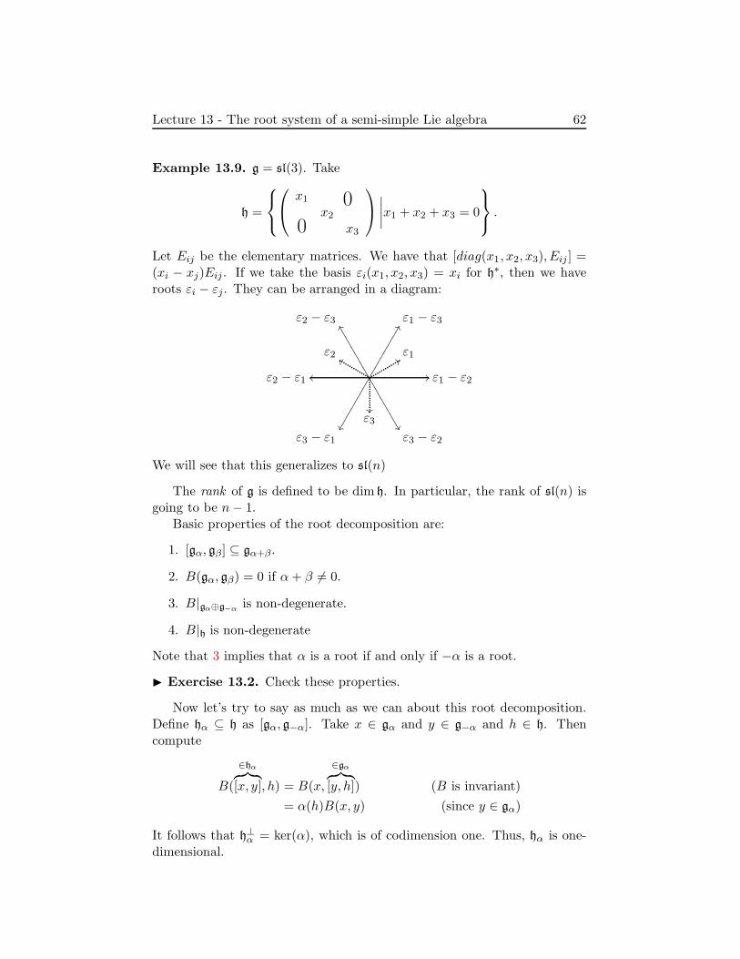
Lecture 13 - The root system of a semi-simple Lie algebra 62
Example 13.9. g = sl(3). Take
h =
x1 0x2
0 x3
∣∣∣∣x1 + x2 + x3 = 0
.
Let Eij be the elementary matrices. We have that [diag(x1, x2, x3), Eij ] =(xi − xj)Eij . If we take the basis εi(x1, x2, x3) = xi for h∗, then we haveroots εi − εj. They can be arranged in a diagram:
ε188ε2 ff
ε3
ε1 − ε2//
ε1 − ε3FF ε2 − ε1 oo
ε2 − ε3 XX1111111111
ε3 − ε1
ε3 − ε211
1111
1111
We will see that this generalizes to sl(n)
The rank of g is defined to be dim h. In particular, the rank of sl(n) isgoing to be n− 1.
Basic properties of the root decomposition are:
1. [gα, gβ] ⊆ gα+β.
2. B(gα, gβ) = 0 if α+ β 6= 0.
3. B|gα⊕g−α is non-degenerate.
4. B|h is non-degenerate
Note that 3 implies that α is a root if and only if −α is a root.
Exercise 13.2. Check these properties.
Now let’s try to say as much as we can about this root decomposition.Define hα ⊆ h as [gα, g−α]. Take x ∈ gα and y ∈ g−α and h ∈ h. Thencompute
B(
∈hα︷ ︸︸ ︷
[x, y], h) = B(x,
∈gα︷ ︸︸ ︷
[y, h]) (B is invariant)
= α(h)B(x, y) (since y ∈ gα)
It follows that h⊥α = ker(α), which is of codimension one. Thus, hα is one-dimensional.

Lecture 13 - The root system of a semi-simple Lie algebra 63
Proposition 13.10. If g is semisimple and α is a root, then α(hα) 6= 0.
Proof. Assume that α(hα) = 0. Then pick x ∈ gα, y ∈ g−α such that[x, y] = h 6= 0. If α(h) = 0, then we have that [h, x] = α(h)x = 0, [h, y] = 0.Thus 〈x, y, h〉 is a copy of the Heisenberg algebra, which is solvable (infact, nilpotent). By Lie’s Theorem, adg(x) and adg(y) are simultaneouslyupper triangularizable, so adg(h) = [adg(x), adg(y)] is nilpotent. This isa contradiction because h is an element of the Cartan subalgebra, so it issemisimple.
For each root α, we will take Hα ∈ hα such that α(Hα) = 2 (we canalways scale Hα to get this). We can choose Xα ∈ gα and Yα ∈ g−α such that[Xα, Yα] = Hα. We have that [Hα,Xα] = α(Hα)Xα = 2Xα and [Hα, Yα] =−2Yα. That means we have a little copy of sl(2) ∼= 〈Hα,Xα, Yα〉. Note that
this makes g a representation of sl2 via sl2 → gad→ gl(g).
We normalize α(hα) to 2 so that we get the standard basis of sl2. Thisway, the representations behave well (namely, that various coefficients areintegers). Next we study these representations.
Irreducible finite dimensional representations of sl(2)
Let H,X, Y be the standard basis of sl(2), and let V be an irreducible rep-resentation. By Corollary 13.2, the action of H on V is diagonalizable andthe actions of X and Y on V are nilpotent. By Lie’s Theorem (appliedto the solvable subalgebra generated by H and X), X and H have a com-mon eigenvector v: Hv = λv and Xv = 0 (since X is nilpotent, its onlyeigenvalues are zero). Verify by induction that
HY rv = Y HY r−1v + [H,Y ]Y r−1v =(λ− 2(r − 1)
)Y rv + 2Y rv
= (λ− 2r)Y rv (∗)XY rv = Y XY r−1v + [X,Y ]Y r−1v
= (r − 1)(λ− (r − 1) + 1
)Y r−1v +
(λ− 2(r − 1)
)Y r−1v
= r(λ− r + 1)Y r−1v (†)
Thus, the span of v, Y v, Y 2v, . . . is a subrepresentation, so it must be allof V (since V is irreducible). Since Y is nilpotent, there is a minimal nsuch that Y nv = 0. From (†), we get that λ = n − 1 is a non-negativeinteger. Since v, Y v, . . . , Y n−1v have distinct eigenvalues (under H), theyare linearly independent.
Conclusion: For every non-negative integer n, there is exactly one irre-ducible representation of sl2 of dimension n + 1, and the H-eigenvalues onthat representation are n, n− 2, n − 4, . . . , 2 − n,−n.
Lecture 13 - The root system of a semi-simple Lie algebra 64
Remark 13.11. As a consequence, we have that in a general root decompo-sition, g = h ⊕⊕α∈∆ gα, each root space is one dimensional. Assume thatdim g−α > 1. Consider an sl(2) in g, generated by 〈Xα, Yα,Hα = [Xα, Yα]〉where Yα ∈ g−α and Xα ∈ gα. Then there is some Z ∈ g−α such that[Xα, Z] = 0 (since hα is one-dimensional). Hence, Z is a highest vector withrespect to the adjoint action of this sl(2). But we have that adHα(Z) = −2Z,and the eigenvalue of a highest vector must be positive! This shows that thechoice of Xα and Yα is really unique.
Definition 13.12. Thinking of g as a representation of sl2 = 〈Xα, Yα,Hα〉,the irreducible subrepresentation containing gβ is called the α-string throughβ.
Let ∆ denote the set of roots. Then ∆ is a finite subset of h∗ with thefollowing properties:
1. ∆ spans h∗.
2. If α, β ∈ ∆, then β(Hα) ∈ Z, and β −(β(Hα)
)α ∈ ∆.
3. If α, cα ∈ ∆, then c = ±1.
Exercise 13.3. Prove these properties.
Lecture 14 - More on Root Systems 65
Lecture 14 - More on Root Systems
Assume g is semisimple. Last time, we started with a regular element h ∈ gssand constructed the decomposition g = h⊕⊕α∈∆ gα, where ∆ ⊆ h∗ is the setof roots. We proved that each gα is one dimensional (we do not call 0 a root).For each root, we associated an sl(2) subalgebra. Given Xα ∈ gα, Yα ∈ g−α,we set Hα = [Xα, Yα], and normalized so that α(Hα) = 2.
Furthermore, we showed that
1. ∆ spans h∗,
2. α(Hβ) ∈ Z, with α− α(Hβ)β ∈ ∆ for all α, β ∈ ∆, and
3. if α, kα ∈ ∆, then k = ±1.
How unique is this decomposition? We started with some choice of aregular semisimple element. Maybe a different one would have produced adifferent Cartan subalgebra.
Theorem 14.1. Let h and h′ be two Cartan subalgebras of a semisimpleLie algebra g (over an algebraically closed field of characteristic zero). Thenthere is some φ ∈ AdG such that φ(h) = h′. Here, G is the Lie groupassociated to g.
Proof. Consider the map
Φ : hreg × gα1 × · · · × gαN→ g
(h, x1, . . . , xN ) 7→ exp(adx1) · · · exp(adxN)h.
Note that adxih is linear in both xi and h, and each adgαiis nilpotent, so
the power series for exp is finite. It follows that Φ is a polynomial function.Since d
dt exp(adtxi)h∣∣t=0
= αi(h)xi ∈ gαi , the differential if Φ at (h, 0, . . . , 0)is
DΦ|(h,0,...,0) =
Idh 0
α1(h) 00
. . .
0 αN (h)
with respect to the decomposition g = h ⊕ gα1 ⊕ · · · ⊕ gαN. DΦ|(h,0,...,0) is
non-degenerate because h ∈ hreg implies that αi(h) 6= 0. So im Φ containsa Zariski open set. Let Φ′ be the analogous map for h′. Since Zariskiopen sets are dense, we have that im Φ ∩ im Φ′ 6= 0. So there is someψ ∈ AdG,ψ′ ∈ AdG, and h ∈ h, h′ ∈ h′ such that ψ(h) = ψ′(h′). Thus, wehave that h = ψ−1ψ′(h).
Lecture 14 - More on Root Systems 66
Abstract Root systems
We’d like to forget that any of this came from a Lie algebra. Let’s just studyan abstract set of vectors in h∗ satisfying some properties. We know that Bis non-degenerate on h, so there is an induced isomorphism s : h → h∗. Bydefinition, 〈s(h), h′〉 = B(h, h′).
Let’s calculate
〈sHβ,Hα〉 = B(Hβ,Hα) = B(Hα,Hβ) (B symmetric)
= B(Hα, [Xβ , Yβ ]) = B([Hα,Xβ ], Yβ) (B invariant)
= B(Xβ , Yβ)β(Hα)
=1
2B([Hβ,Xβ], Yβ)β(Hα) (2Xβ = [Hβ,Xβ ])
=1
2B(Hβ,Hβ)β(Hα) (B invariant)
Thus, we have that s(Hβ) =B(Hβ ,Hβ)
2 β. Also, compute
(β, β) := 〈β, s−1β〉
= β
(2Hβ
B(Hβ,Hβ)
)
=4
B(Hβ,Hβ)(β(Hβ) = 2)
So s(Hβ) = 2β(β,β) . This is sometimes called the coroot of β, and denoted β.
Thus, we may rewrite fact 2 from last time as:
For α, β ∈ ∆,2(α, β)
(β, β)∈ Z, and α− 2(α, β)
(β, β)β ∈ ∆. (2′)
Now you can define rβ : h∗ → h∗ given by rβ(x) = x − 2(x,β)(β,β) β. This is
the reflection through the hyperplane orthogonal to β in h∗. The groupgenerated by the rβ for β ∈ ∆ is a Coxeter group. If we want to study thesethings, we’d better classify root systems.
We want to be working in Euclidean space, but we are now in h∗. Let hrbe the real span of the Hα’s. We claim that B is positive definite on hr. Tosee this, note that Xα, Yα,Hα make a little sl(2) in g, and that g is thereforea representation of sl(2) via the adjoint actions adXα , adYα , adHα . But weknow that in any representation of sl(2), the eigenvalues of Hα must beintegers. Thus, adHα adHα has only positive eigenvalues, so B(Hα,Hα) =tr(adHα adHα) > 0.
Thus, we may think of our root systems in Euclidean space, where the
inner product on h∗ is given by (µ, ν)def= B(s−1(µ), s−1(ν)) = 〈µ, s−1ν〉.

Lecture 14 - More on Root Systems 67
Definition 14.2. An abstract reduced root system is a finite set ∆ ⊆ Rn r0 which satisfies
(RS1) ∆ spans Rn,
(RS2) for α, β ∈ ∆, 2(α,β)(β,β) ∈ Z, with rβ(∆) = ∆
(i.e. α, β ∈ ∆ ⇒ rβ(α) ∈ ∆, with α− rβ(α) ∈ Zβ ), and
(RS3) α, kα ∈ ∆ ⇒ k = ±1 (this is the “reduced” part).
The number n is called the rank of ∆.
Notice that given root systems ∆1 ⊂ Rn,∆2 ⊂ Rm, we have that∆1∐
∆2 ⊂ Rn ⊕ Rm is a root system.
Definition 14.3. A root system is irreducible if it cannot be decomposedinto the union of two systems of smaller rank.
Exercise 14.1. Let g be a semisimple Lie algebra and let ∆ be its rootsystem. Show that ∆ is irreducible if and only if g is simple.
Now we will classify all systems of rank 2. Observe that 2(α,β)(α,α)
2(α,β)(β,β) =
4cos2 θ, where θ is the angle between α and β. This thing must be aninteger. Thus, there are not many choices for θ:
cos θ 0 ±12 ± 1√
2±
√3
2
θ π2
π3 ,
2π3
π4 ,
3π4
π6 ,
5π6
Choose two vectors with minimal angle between them. If the minimal angleis π/2, then the system is reducible.
α//oo
βOO
Notice that α and β can be scaled independently.If the minimal angle is smaller than π/2, then rβ(α) 6= α, so the difference
α− rβ(α) is a non-zero integer multiple of β (in fact, a positive multiple ofβ since θ < π/2). If we assume ‖α‖ ≤ ‖β‖ (we can always switch them),we get that ‖α − rβ(α)‖ < 2‖α‖ ≤ 2‖β‖, so α− rβ(α) = β. Thus, once weset the direction of β, its length is determined (relative to α). Then we canobtain the remaining elements of the root system from the condition that∆ is invariant under rα and rβ, observing that no additional vectors can be
Lecture 14 - More on Root Systems 68
added without violating RS2, RS3, or the prescribed minimal angle. Thus,all the irreducible rank two root systems are
A2, θ = π/3 B2, θ = π/4 G2, θ = π/6
α//
βFF
XX1111111oo
rβ(α)11
1111
1
α//
β??
OO__?????????oo
rβ(α)
????
????
? α//
ffMMMMMMMM
XX11111
FF
β88qqqqqqqq
OO
oo
&&MMMMMMMM
11
111
rβ(α)
xxqqqqqqqq
The Weyl group
Given a root system ∆ = α1, . . . , αN, we call the group generated by therαis the Weyl group, denoted W .
Remark 14.4. Each rα ∈ W can be constructed in terms of the group G ofg. If you have Xα, Yα,Hα generating an sl(2), then you know that there isa subgroup SL(2) of G . There is a special element corresponding to
(0 1−1 0
)
in there. It is given by sα = exp(Xα) exp(−Yα) exp(Xα). We have that〈β,Adsα(h)〉 = 〈rαβ, h〉 . So this reflection is coming from the embeddingof SL(2) in G.
Exercise 14.2. Let g be a semisimple Lie algebra, and let h be a Cartansubalgebra. For each root α define
sα = exp(adXα) exp(−adYα) exp(adXα).
Prove that sα(h) = h and
〈λ, sα(h)〉 = 〈rα(λ), h〉
for any h ∈ h and λ ∈ h∗, where rα is the reflection in α⊥.
Example 14.5. The root system An is the root system of sln+1. We pickan orthonormal basis ε1, . . . , εn+1 of Rn+1, the the root system is the set ofall the differences: ∆ = εi − εj |i 6= j. We have that
rεi−εj(εk) =
εk k 6= i, jεj k = iεi k = j
is a transposition, so we have that W ≃ Sn+1
Now back to classification of abstract root systems.Draw a hyperplane in general position (so that it doesn’t contain any
roots). This divides ∆ into two parts, ∆ = ∆+∐
∆−. The roots in ∆+
Lecture 14 - More on Root Systems 69
are called positive roots, and the elements of ∆− are called negative roots.We say that α ∈ ∆+ is simple if it cannot be written as the sum of otherpositive roots. Let Π be the set of simple roots, sometimes called a base. Ithas the properties
1. Any α ∈ ∆+ is a sum of simple roots (perhaps with repitition): α =∑
β∈Πmββ where mβ ∈ Z≥0.
2. If α, β ∈ Π, then (α, β) ≤ 0.
This follows from the fact that if (α, β) > 0, then α− β and β−α areagain roots (as we showed when we classified rank 2 root systems), andone of them is positive, say α−β. Then α = β+(α−β), contradictingsimplicity of α.
3. Π is a linearly independent set.
If they were linearly dependent, the relation∑
αi∈Π aiαi = 0 musthave some negative coefficients (because all of Π is in one half space),so we can always write
0 6= a1α1 + · · · + arαr = ar+1αr+1 + · · · + anαn
with all the ai ≥ 0. Taking the inner product with the left hand side,we get
‖a1α1+ · · · + arαr‖2
= (a1α1 + · · · + arαr, ar+1αr+1 + · · · + anαn) ≤ 0
by 2, which is absurd.
Remark 14.6. Notice that the hyperplane is t⊥ for some t, and the positiveroots are the α ∈ ∆ for which (t, α) > 0. This gives an order on the roots.You can inductively prove 1 using this order.
Remark 14.7. Notice that when you talk about two roots, they always gen-erate one of the rank 2 systems, and we know what all the rank 2 systemsare.
Claim. Suppose we have chosen ∆+ ⊃ Π. Then for α ∈ Π, we have thatrα(∆+) = ∆+ ∪ −α r α.
Proof. For β 6= α simple, we have rα(β) = β + kα for some non-negative k;this must be on the positive side of the hyperplane, so it is a positive root.Now assume you have a positive root of the form γ = mα +
∑
αi 6=αmiαi,with m,mi ≥ 0. Then we have that rα(γ) = −mα +
∑m′iαi ∈ ∆. If
any of the mi were non-zero, we know that some m′i is positive (by the
Lecture 14 - More on Root Systems 70
base case above), but every root can be (uniquely) written as either a non-negative or a non-positive combination of the simple roots. Since rα(γ) hassome positive coefficient, it must be a non-negative combination, so it is apositive root.
Suppose we have two different sets of positive roots ∆+ and ∆+1 , then
one can get ∆+1 from ∆+ by a chain of simple reflections. You have to be
a little careful because the set of simple roots changes, so you’re pickingyour reflections from different sets. Fix a base Π = α1, . . . , αn, and callri := rαi simple reflections.
Proposition 14.8. Simple reflections act transitively on the set of sets ofpositive roots.
Proof. Start with ∆+, and apply ri to get a new ∆+1 , then from the new
base apply some rα to get ∆+2 , so you have ∆+
2 = rαri∆+. The important
thing is that for any element of the Weyl group, we have wrαw−1 = rwα. So
if α = ri(αj), we have that rαri = rirj . Induct.
Corollary 14.9. W is generated by simple reflections.
Proof. Any root is a simple root for some choice of positive roots. To showthis, draw your hyperplane really close to your vector. Then we know thatα is obtained from our initial set Π by simple reflections. We get that ifα = ri1 · · · rik(αj), then rα = (ri1 · · · rik)rj(ri1 · · · rik)−1.
Let’s see how it works for An. Choose a vector t = t1ε1 + · · ·+ tn+1εn+1
in such a way that t1 > · · · > tn+1. Then we have that (εi − εj , t) = ti − tj,so the positive roots are the εi − εj for which i < j. Then the simple rootsare Π = ε1 − ε2, . . . , εn − εn+1

Lecture 15 - Dynkin diagrams, Classification of root systems 71
Lecture 15 - Dynkin diagrams, Classification of root
systems
Last time, we talked about root systems ∆ ⊂ Rn. We constructed the Weylgroup W , the finite group generated by reflections. We considered Π ⊂ ∆,the simple roots. Π forms a basis for Rn, and showed that every root is anon-negative (or non-positive) linear combination of simple roots.
We showed that if you have α, β ∈ Π, then nαβ = 2(α,β)(β,β) ∈ Z≤0. There
are not many options for this value. It can only be 0,−1,−2, or −3. Also,we have that nαβnβα = 4cos2 θαβ. If nαβ = 0, the two are orthogonal. Ifnαβ = −1, then the angle must be 2π/3 and the two are the same length.If nαβ = −2, the angle must be 3π/4 and ||β|| =
√2 ||α||. If nαβ = −3, the
angle is 5π/6 and ||β|| =√
3 ||α||. Thus we get:
nβα nαβ relationship Dynkin picture
0 0 α//
βOO
α β
−1 −1 α//
βXX111
α β
−2 −1 α//β __?????
α β oo
−3 −1 α//β ffMMMMM α β oo
We will encode this information in a Dynkin diagram. The nodes of thediagram are simple roots. We join two nodes by nαβnβα lines. The arrowsgo from the longer root to the shorter root in the case of two or three lines.(As always, the alligator eats the big one.)
There is also something called a Coxeter diagram, which is not directed.You look at ei = α
(α,α)1/2 , i = 1, ..., n. Then the number of lines between two
vertices is nαβnβα = 4 · (α,β)2
(α,α)(β,β) = 4(ei, ej)2.
Example 15.1. An has n simple roots, given by εi − εi+1. So the graphsare
Dynkin ... Coxeter • • ... • •
Properties of the Coxeter graph:
(CX1) A subgraph of a Coxeter graph is a Coxeter graph. This is trivial.
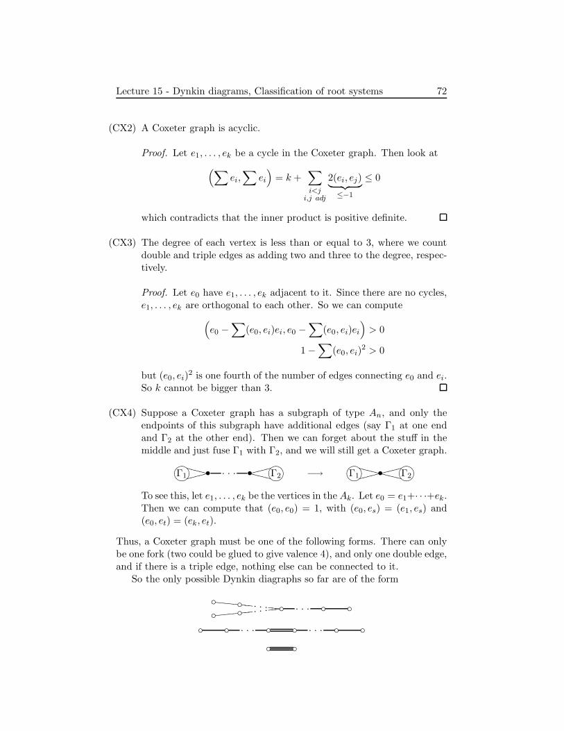
Lecture 15 - Dynkin diagrams, Classification of root systems 72
(CX2) A Coxeter graph is acyclic.
Proof. Let e1, . . . , ek be a cycle in the Coxeter graph. Then look at
(∑
ei,∑
ei
)
= k +∑
i<ji,j adj
2(ei, ej)︸ ︷︷ ︸
≤−1
≤ 0
which contradicts that the inner product is positive definite.
(CX3) The degree of each vertex is less than or equal to 3, where we countdouble and triple edges as adding two and three to the degree, respec-tively.
Proof. Let e0 have e1, . . . , ek adjacent to it. Since there are no cycles,e1, . . . , ek are orthogonal to each other. So we can compute
(
e0 −∑
(e0, ei)ei, e0 −∑
(e0, ei)ei
)
> 0
1 −∑
(e0, ei)2 > 0
but (e0, ei)2 is one fourth of the number of edges connecting e0 and ei.
So k cannot be bigger than 3.
(CX4) Suppose a Coxeter graph has a subgraph of type An, and only theendpoints of this subgraph have additional edges (say Γ1 at one endand Γ2 at the other end). Then we can forget about the stuff in themiddle and just fuse Γ1 with Γ2, and we will still get a Coxeter graph.
Γ18?9>:=;< • ... • Γ2
8?9>:=;<WWWWWggggg WWWWW
ggggg −→ Γ18?9>:=;< • Γ2
8?9>:=;<WWWWWgggggWWWWW
ggggg
To see this, let e1, . . . , ek be the vertices in the Ak. Let e0 = e1+· · ·+ek.Then we can compute that (e0, e0) = 1, with (e0, es) = (e1, es) and(e0, et) = (ek, et).
Thus, a Coxeter graph must be one of the following forms. There can onlybe one fork (two could be glued to give valence 4), and only one double edge,and if there is a triple edge, nothing else can be connected to it.
So the only possible Dynkin diagraphs so far are of the form
\\\\\ \\\ ... \\\bbb. . . bbb bbbbb ... ... ...

Lecture 15 - Dynkin diagrams, Classification of root systems 73
Now we use the property that a subgraph of a Dynkin graph is a Dynkingraph. Now we will calculate that some things are forbidden. We label thevertex corresponding to αi with a number mi, and check that
(∑
miαi,∑
miαi
)
= 0.
1 2 3 4 // 2 1 2 3 2 oo 1 1 2 3
2
1
2 1 1 2 3 4
2
3 2 1
2 4 6
3
5 4 3 2 1
Thus we have narrowed our list of possible Dynkin diagrams to a shortlist.
Connected Dynkin diagrams: n is the total number of vertices.
... (An)
... // (Bn)
... oo (Cn)
... nnnnn
PPPPP (Dn)
Those are the “classical diagrams”, and the others are
// (G2)
// (F4)
(E6)
(E7)
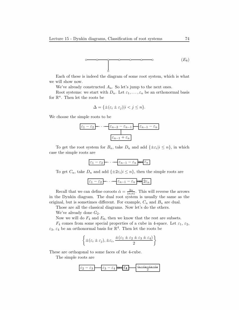
Lecture 15 - Dynkin diagrams, Classification of root systems 74
(E8)
Each of these is indeed the diagram of some root system, which is whatwe will show now.
We’ve already constructed An. So let’s jump to the next ones.Root systems: we start with Dn. Let ε1, . . . , εn be an orthonormal basis
for Rn. Then let the roots be
∆ = ±(εi ± εj)|i < j ≤ n.
We choose the simple roots to be
ε1 − ε2 ... εn−2 − εn−1
εn−1 + εn
εn−1 − εn
To get the root system for Bn, take Dn and add ±εi|i ≤ n, in whichcase the simple roots are
ε1 − ε2 ... εn−1 − εn εn//
To get Cn, take Dn and add ±2εi|i ≤ n, then the simple roots are
ε1 − ε2 ... εn−1 − εn 2εnoo
Recall that we can define coroots α = 2α(α,α) . This will reverse the arrows
in the Dynkin diagram. The dual root system is usually the same as theoriginal, but is sometimes different. For example, Cn and Bn are dual.
Those are all the classical diagrams. Now let’s do the others.We’ve already done G2.Now we will do F4 and E8, then we know that the rest are subsets.F4 comes from some special properties of a cube in 4-space. Let ε1, ε2,
ε3, ε4 be an orthonormal basis for R4. Then let the roots be
±(εi ± εj),±εi,±(ε1 ± ε2 ± ε3 ± ε4)
2
These are orthogonal to some faces of the 4-cube.The simple roots are
ε2 − ε3 ε3 − ε4 ε4// ε4 ε1−ε2−ε3−ε42

Lecture 15 - Dynkin diagrams, Classification of root systems 75
There are 48 roots total. Remember that the dimension of the lie algebra isthe number of roots plus the dimension of the cartan (the rank of g, whichis 4 here), so the dimension is 52 in this case.
Construction of E8. Look at R9 with our usual orthonormal basis. Thetrick is that we are going to project on to the plane orthogonal to ε1+· · ·+ε9(so just throw in the relation that that sum is 0, so that we work in thehyperplane). The roots are
εi − εj |i 6= j ∪ ±(εi + εj + εk)|i 6= j 6= k
The total number of roots is |∆| = 9 · 8 + 2(93
)= 240. So the dimension of
the algebra is 248! The simple roots are
ε1 − ε2 ε2 − ε3 ε3 − ε4 ε4 − ε5 ε5 − ε6
ε6 + ε7 + ε8
ε6 − ε7 ε7 − ε8
These are all the indecomposable root systems, the rest are just directsums.
Theorem 15.2 (Serre). Say k algebraically closed, characteristic 0. Foreach indecomposable root system, there exists (unique up to isomorphism) asimple Lie algebra with the given root system.
There are several ways to do this. You could construct all of themexplicitly. The other way is to use Serre’s relations, which is what we willdo later.
Let’s construct the Lie algebras for An, Bn, Cn,Dn. We know that An issl(n+ 1). Let’s consider so(2n), the linear maps of k2n preserving the form.We can choose a basis for k2n so that the matrix of the form is I =
(0 1n1n 0
).
Let X ∈ so(2n), then we have that XtI + IX = 0. So we can write
X =
(A BC −At
)
Where Bt = −B,Ct = −C. What should the Cartan subalgebra be? Itshould be a maximal abelian subalgebra. Notice that if we take A =diag(t1, . . . , tn) to be diagonal and B = C = 0, then we get an abeliansubalgebra h. What are the root spaces? We have that Eij − Ej+n,i+n haseigenvalue ti − tj . We have that Ei,j+n − Ej,i+n has eigenvalue ti + tj , andthe symmetric term with eigenvalue −ti− tj. So we get the root system Dn.
Now let’s look at sp(2n), the linear operators which preserve a non-degenerate skew-symmetric form. In some basis, the form is J =
(0 1n
−1n 0
),
with XtJ + JX = 0. We get the same conditions, except that B = Bt, C =
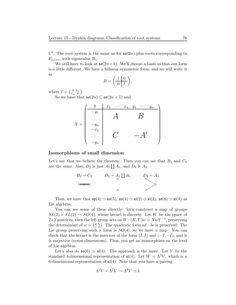
Lecture 15 - Dynkin diagrams, Classification of root systems 76
Ct. The root system is the same as for so(2n) plus roots corresponding toEi,i+n, with eigenvalue 2ti.
We still have to look at so(2n+1). We’ll choose a basis so that our formis a little different. We have a bilinear symmetric form, and we will write itas
B =
(1 0
0 I
)
,
where I =(
0 1n1n 0
).
So we have that so(2n) ⊆ so(2n + 1) and
X =
0 x1 · · · xn y1 · · · yn−y1
...−yn−x1
...−yn
A B
C −At
Isomorphisms of small dimension
Let’s say that we believe the theorem. Then you can see that B2 and C2
are the same. Also, D2 is just A1∐A1, and D3 is A3:
B2 = C2 D2 = A1∐A1 D3 = A3
//
qqqqq
MMMMM
Thus, we have that sp(4) ≃ so(5), so(4) ≃ sl(2) ⊕ sl(2), so(6) ≃ sl(4) asLie algebras.
You can see some of these directly: let’s construct a map of groupsSL(2) × SL(2) → SO(4), whose kernel is discrete. Let W be the space of2×2 matrices, then the left group acts onW : (X,Y )w = XwY −1, preservingthe determinant of w =
(a bc d
). The quadratic form ad−bc is preserved. The
Lie group preserving such a form is SO(4), so we have a map. You cancheck that the kernel is the matrices of the form (I, I) and (−I,−I), and itis surjective (count dimensions). Thus, you get an isomorphism on the levelof Lie algebras.
Let’s also do so(6) ≃ sl(4). The approach is the same. Let V be thestandard 4-dimensional representation of sl(4). Let W = Λ2V , which is a6-dimensional representation of sl(4). Note that you have a pairing
Λ2V × Λ2V → Λ4V ≃ k

Lecture 15 - Dynkin diagrams, Classification of root systems 77
where the last isomorphism is as representations of SL(4) (because determi-nant is 1 in SL(4)). Thus, W = Λ2V has some SL(4)-invariant symmetricbilinear form which is preserved, so you get a map SL(4) → SO(6). It isnot hard to check that the kernel is ±I, and the dimensions match, so it issurjective. Thus, you get an isomorphism of Lie algebras.
Next time, we’ll do this theorem and we’ll talk about the Exceptionalalgebras.

Lecture 16 - Serre’s Theorem 78
Lecture 16 - Serre’s Theorem
Today we’re going to prove Serre’s theorem, and then work with some con-structions of the exceptional algebras.
Start with a semi-simple Lie algebra g (over k = k), with Cartan subal-gebra h ⊂ g. Then we have the root system ∆, with a fixed set of simpleroots Π = α1, . . . , αn. We have Xi := Xαi , Yi,Hi associated to each simpleroot.
The Cartan matrix is aij = αj(Hi) =2(αi,αj)(αi,αi)
. We know that αij ∈ Z≤0
for i 6= j and aii = 2.Then we claim that the following relations are satisfied:
[Hi,Hj] = 0 [Hi,Xj ] = aijXj [Hi, Yj ] = −aijYj [Xi, Yj] = δijHi (1)
(θ+ij) (adXi)
1−aijXj = 0 (adYi)1−aijYj = 0 (θ−ij) (2)
the second group are called Serre’s relations (though Serre called them Weylrelations). We verify that these relations hold in our Lie algebra.
The tricky one from (1) is that [Xi, Yj] = 0 when i 6= j. You know that[gαi , g−αj ] ⊆ gαi−αj , but αi − αj 6∈ ∆! So gαi−αj = 0.
Example 16.1. g = sl(n + 1). We have Xi = Ei,i+1, Yi = Ei+1,i,Hi =[Xi, Yi] = Eii − Ei+1,i+1.
Let’s check that the second group of relations hold. We want to showthat (adXi)
1−aijXj = 0. What is aij? We know that (adXi)1−ai,i+1Xi+1 = 0
by a calculation ... just do it.
To see why these relations hold in general, consider θ−ij . We have thatadXi(Yj) = 0, so Yj is a highest vector with respect to this sl(2) action. Wealso have that adHi(Yj) = −aijYj , so the highest weight is −aij. We knowwhat representations of sl(2) look like, so we know that (adYi)
1−aijYj = 0.Thus, θ−ij holds. To show θ+
ij , you can switch Xi and Yi, and negate Hi.We don’t know that these are all the relations yet. We also do not yet
know that for every root system there is an algebra. But we know that ifsuch an algebra exists, then it satisfies these relations.
Theorem 16.2. Let g be the Lie algebra with generators Hi,Xi, Yi for 1 ≤i ≤ n, with a Cartan matrix aij = (αi, αj) from some root system and therelations given, then g is a finite dimensional semi-simple Lie algebra withthe Cartan subalgebra spanned by H1, . . . ,Hn, and with the given root system∆.
Note that this shows existence. But since any such Lie algebra satisfiesthese relations, we have uniqueness (you cannot add more relations withoutmaking the root system smaller).

Lecture 16 - Serre’s Theorem 79
Remark 16.3. When we talk about a Lie algebra with some generators andrelations, how do you think about it? What is a free Lie algebra? It istricky to think about the Jacobi identity, not like in an associative algebra.But a Lie algebra always has an associative algebra Ug. What is Ug goingto be? The free associative algebra with the same generators . If you havegenerators g1, . . . , gn, look at the tensor algebra T (g1, . . . , gn), and realize g
inside as a Lie subalgebra generated by g1, . . . , gn.
Proof. Step 1: Take the free Lie algebra and quotient by the relations ingroup (1). Call the result g. Then the claim is that
g = n− ⊕ h ⊕ n+
as vector spaces, where h is the abelian Lie algebra generated by H1, . . . ,Hn,and n± are free Lie algebras generated by the Xi (resp. Yi). They shouldbe free because there are no relations among the Xi’s, but it is not so easy.There is a standard trick for doing such things.
U g = U(n−)U(h)U(n+) (easy to show from relations (1)). In fact, wewant U(g) = U(n−)
︸ ︷︷ ︸
T (n−)
⊗U(h)︸ ︷︷ ︸
S(h)
⊗U(n+)︸ ︷︷ ︸
T (n+)
. We construct a representation of g in
T (n−) ⊗ S(h).We say Yi(1⊗ 1) = Yi⊗ 1, h(1⊗ 1) = 1⊗ h, and Xi(1⊗ 1) = 0. Then we
define things inductively:
Yi(Yja⊗ b) =def YiYja⊗ b
Hi(Yja⊗ b) = Yj(Hi(a⊗ b)) − aijYj(a⊗ b)
Xi(Yja⊗ b) = Yj(Xi(a⊗ b)) + δijHi(a⊗ b)
Your job is to check that this gives a representation (note that 1⊗1 generatesthe whole representation).
So we get an isomorphism of U(n−) and T (n−). We define U(n− + h)ևT (n−) ⊗ S(h) given by x 7→ x(1 ⊗ 1). We do the same thing for n+.
0 → U(n+) → U(g) → T (n−) ⊗ S(h) → 0
0 → U(n−) → U(g) → T (n+) ⊗ S(h) → 0
Hence U(g) ≃ T (n−) ⊗ S(h) ⊗ T (n+). So g = n− ⊕ h ⊕ n+.Step 2: We now throw in relations from group (2). We have that θ±ij ∈
n±. We have to verify that[Yk, θ
+ij ] = 0
which sort of follows from relations from group (1) (check for yourself). Wehave that
[Hk, θ+ij ] = ckijθ
+ij
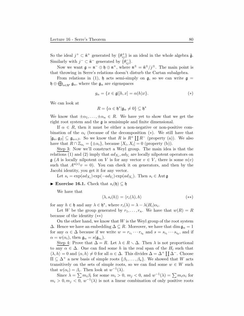
Lecture 16 - Serre’s Theorem 80
So the ideal j+ ⊂ n+ generated by θ+ij is an ideal in the whole algebra g.
Similarly with j− ⊂ n− generated by θ−ij.Now we want g = n− ⊕ h ⊕ n+, where n± = n±/j±. The main point is
that throwing in Serre’s relations doesn’t disturb the Cartan subalgebra.From relations in (1), h acts semi-simply on g, so we can write g =
h ⊕⊕α∈h∗ gα, where the gα are eigenspaces
gα = x ∈ g|[h, x] = α(h)x. (∗)
We can look atR = α ∈ h∗|gα 6= 0 ⊆ h∗
We know that ±α1, . . . ,±αn ∈ R. We have yet to show that we get theright root system and the g is semisimple and finite dimensional.
If α ∈ R, then it must be either a non-negative or non-positive com-bination of the αi (because of the decomposition (∗). We still have that[gα, gβ] ⊆ gα+β. So we know that R is R+
∐R− (property (a)). We also
have that R ∩ Zαi = ±αi, because [Xi,Xi] = 0 (property (b)).Step 3: Now we’ll construct a Weyl group. The main idea is that the
relations (1) and (2) imply that adXi , adYi are locally nilpotent operators ong (A is locally nilpotent on V is for any vector v ∈ V , there is some n(v)such that An(v)v = 0). You can check it on generators, and then by theJacobi identity, you get it for any vector.
Let si = exp(adXi) exp(−adYi) exp(adXi). Then si ∈ Aut g
Exercise 16.1. Check that si(h) ⊆ h
We have that〈λ, si(h)〉 = 〈ri(λ), h〉 (∗∗)
for any h ∈ h and any λ ∈ h∗, where ri(λ) = λ− λ(Hi)αi.Let W be the group generated by r1, . . . , rn. We have that w(R) = R
because of the identity (∗∗)On the other hand, we know that W is the Weyl group of the root system
∆. Hence we have an embedding ∆ ⊆ R. Moreover, we have that dim gα = 1for any α ∈ ∆ because if we write w = ri1 · · · rik and s = si1 · · · sik , and ifα = w(αi), then gα = s(gαi).
Step 4: Prove that ∆ = R. Let λ ∈ R r∆. Then λ is not proportionalto any α ∈ ∆. One can find some h in the real span of the Hi such that〈λ, h〉 = 0 and 〈α, h〉 6= 0 for all α ∈ ∆. This divides ∆ = ∆+
∐∆−. Choose
Π ⊆ ∆+ a new basis of simple roots β1, . . . , βn. We showed that W actstransitively on the sets of simple roots, so we can find some w ∈ W suchthat w(αi) = βi. Then look at w−1(λ).
Since λ =∑miβi for some mi > 0, mj < 0, and w−1(λ) =
∑miαi for
mi > 0,mj < 0, w−1(λ) is not a linear combination of only positive roots
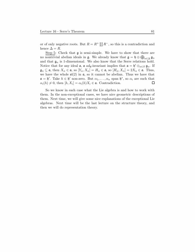
Lecture 16 - Serre’s Theorem 81
or of only negative roots. But R = R+∐R−, so this is a contradiction and
hence ∆ = R.Step 5: Check that g is semi-simple. We have to show that there are
no nontrivial abelian ideals in g. We already know that g = h ⊕⊕α∈∆ gαand that gα is 1-dimensional. We also know that the Serre relations hold.Notice that for any ideal a, a adh-invariant implies that a = h′ ⊕α∈S gα. Ifgα ⊆ a, then Xα ∈ a, so [Yα,Xα] = Hα ∈ a, so [Hα,Xα] = 2Xα ∈ a. Thus,we have the whole sl(2) in a, so it cannot be abelian. Thus we have thata = h′. Take h ∈ h′ non-zero. But α1, . . . , αn span h∗, so αi are such thatαi(h) 6= 0, then [h,Xi] = αi(h)Xi ∈ a. Contradiction.
So we know in each case what the Lie algebra is and how to work withthem. In the non-exceptional cases, we have nice geometric descriptions ofthem. Next time, we will give some nice explanations of the exceptional Liealgebras. Next time will be the last lecture on the structure theory, andthen we will do representation theory.

Lecture 17 - Constructions of Exceptional simple Lie Algebras 82
Lecture 17 - Constructions of Exceptional simple
Lie Algebras
We’ll begin with the construction of G2. Consider the picture
v1• w2• v3•
w3•
v2•
w1•u•
1111
1111
1111
1111
1
qqqqqqqqqqqqqqq MMMMMMMMMMMMMMM
This is the projective plane over F2.Consider the standard 7-dimensional representation of gl(7), call it E.
Take a basis given by points in the projective plane above.
Exercise 17.1. Prove that Λ3E has an open gl(7)-orbit, by looking atthe particular vector
ω = v1 ∧ v2 ∧ v3 +w1 ∧ w2 ∧ w3 + u ∧ v1 ∧ w1 + u ∧ v2 ∧ w2 + u ∧ v3 ∧ w3
and checking that gl(7)ω = Λ3E. (Remember x(v1 ∧ v2) = x(v1)∧ v2 + v1 ∧x(v2). )
Claim. g = x ∈ gl(7)|xω = 0 is a simple Lie algebra with root system G2.
Proof. We have to choose a Cartan subalgebra of this g. Consider linearoperators which are diagonal in the given basis u, v1, v2, v3, w1, w2, w3, takeh = diag(c, a1, a2, a3, b1, b2, b3). We want that hω = 0, which gives somelinear equations. It is easy to check that hω = 0 implies that c = 0, a1 +a2 + a3 = 0, and bi = −ai. This is a 2-dimensional subalgebra, it is ourCartan subalgebra.
If you consider the root diagram for G2 and look at only the long roots,you get a copy of A2. This should mean that you have an embedding A2 ⊆G2, so we should look for a copy of sl(3) in our g. We can write E =ku⊕V ⊕W , where V = 〈v1, v2, v3〉 and W = 〈w1, w2, w3〉. Let’s consider thesubalgebra which not only kills ω, but also kills u. Let g0 = x ∈ g|xu = 0.For x ∈ g0 we have x(v1∧v2∧v3) = 0 and x(w1∧w2∧w3) = 0, so x preservesV and W . It also must kill the 2-form α = v1 ∧w1 + v2 ∧w2 + v3 ∧w3, since0 = x(u ∧ α) = xu ∧ α+ u ∧ xα = u ∧ xα forces xα = 0. This 2-form givesa pairing, so that V ≃ W ∗. We can compute exactly what the pairing is,〈vi, wj〉 = δij . Therefore the operator x must be of the form
x =
0 0 0
0 A 00 0 −At

Lecture 17 - Constructions of Exceptional simple Lie Algebras 83
[[where A has trace zero?]]The total dimension of G2 is 14, which we also know by the exercise is
the dimension of g. We saw the Cartan subalgebra has dimension 2, andthis g0 piece has dimension 6. So we still need another 6 dimensional piece.
For each v ∈ V , define a linear operator Xv which acts by Xv(u) = v.Λ2V ≃γ W is dual to V (since Λ3V = C). ThenXv acts byXv(v
′) = γ(v∧v′)and Xv(w) = 2〈v,w〉u. Check that this kills α, and hence is in g.
Similarly, you can define Xw for each w ∈ W by Xw(u) = w,Xw(w′) =γ(w ∧w′),Xw(v) = 2〈w, v〉u.
If you think about a linear operator which takes u 7→ vi, it must be insome root space, this tells you about how it should act on V and W . Thisis how we constructed Xv and Xw, so we know that Xvi and Xwi are insome root spaces. We can check that their roots are the short roots in thediagram,
Xv188qqqqqqoo
Xv2ffMMMMMM
Xw3OO
FF
XX1111111111
Xw1xxqqqqqq //
Xw2&&M
MMMMM
Xv3
11
1111
1111
and so they span the remaining 6 dimensions of G2. To properly completethis construction, we should check that this is semisimple, but we’re notgoing to.
We saw here that G2 is isomorphic to the Lie algebra of automorphismsof a generic 3-form in 7-dimensional space. The picture of the projectiveplane is related to Cayley numbers, an important nonassociative divisionalgebra, of which G2 is the algebra of automorphisms.
Let’s analyze what we did with G2, so that we can do a similar thingto construct E8. We discovered certain phenomena, we can write g =g0︸︷︷︸
sl(3)
⊕ g1︸︷︷︸
V
⊕ g2︸︷︷︸
W
. This gives us a Z/3-grading: [gi, gj ] ⊆ gi+j(mod 3). As an
sl(3) representation, it has three components: ad, standard, and the dual tothe standard. We get that W ∼= V ∗ ≃ Λ2V . Similarly, V ≃ Λ2W . This iscalled Triality.
More generally, say we have g0 a semi-simple Lie algebra, and V,W
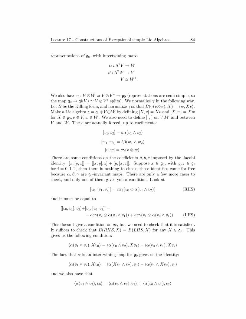
Lecture 17 - Constructions of Exceptional simple Lie Algebras 84
representations of g0, with intertwining maps
α : Λ2V →W
β : Λ2W → V
V ≃W ∗.
We also have γ : V ⊗W ≃ V ⊗V ∗ → g0 (representations are semi-simple, sothe map g0 → gl(V ) ≃ V ⊗V ∗ splits). We normalize γ in the following way.LetB be the Killing form, and normalize γ so thatB(γ(v⊗w),X) = 〈w,Xv〉.Make a Lie algebra g = g0⊕V ⊕W by defining [X, v] = Xv and [X,w] = Xwfor X ∈ g0, v ∈ V,w ∈W . We also need to define [ , ] on V ,W and betweenV and W . These are actually forced, up to coefficients:
[v1, v2] = aα(v1 ∧ v2)
[w1, w2] = bβ(w1 ∧w2)
[v,w] = cγ(v ⊗ w).
There are some conditions on the coefficients a, b, c imposed by the Jacobiidentity; [x, [y, z]] = [[x, y], z] + [y, [x, z]]. Suppose x ∈ g0, with y, z ∈ gifor i = 0, 1, 2, then there is nothing to check, these identities come for freebecause α, β, γ are g0-invariant maps. There are only a few more cases tocheck, and only one of them gives you a condition. Look at
[v0, [v1, v2]] = caγ(v0 ⊗ α(v1 ∧ v2)) (RHS)
and it must be equal to
[[v0, v1], v2]+[v1, [v0, v2]] =
− acγ(v2 ⊗ α(v0 ∧ v1)) + acγ(v1 ⊗ α(v0 ∧ v1)) (LHS)
This doesn’t give a condition on ac, but we need to check that it is satisfied.It suffices to check that B(RHS,X) = B(LHS,X) for any X ∈ g0. Thisgives us the following condition:
〈α(v1 ∧ v2),Xv0〉 = 〈α(v0 ∧ v2),Xv1〉 − 〈α(v0 ∧ v1),Xv2〉
The fact that α is an intertwining map for g0 gives us the identity:
〈α(v1 ∧ v2),Xv0〉 = 〈α(Xv1 ∧ v2), v0〉 − 〈α(v1 ∧Xv2), v0〉
and we also have that
〈α(v1 ∧ v2), v0〉 = 〈α(v0 ∧ v2), v1〉 = 〈α(v0 ∧ v1), v2〉
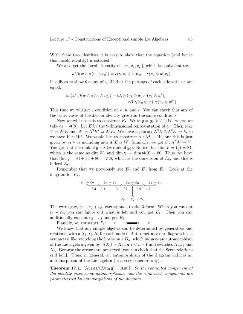
Lecture 17 - Constructions of Exceptional simple Lie Algebras 85
With these two identities it is easy to show that the equation (and hencethis Jacobi identity) is satisfied.
We also get the Jacobi identity on [w, [v1, v2]], which is equivalent to:
abβ(w ∧ α(v1 ∧ v2)) = c(γ(v1 ⊗ w)v2 − γ(v2 ⊗ w)v1)
It suffices to show for any w′ ∈W that the pairings of each side with w′ areequal,
ab〈w′, β(w ∧ α(v1 ∧ v2)〉 = cB(γ(v1 ⊗ w), γ(v2 ⊗ w′))
− cB(γ(v2 ⊗ w), γ(v1 ⊗ w′))
This time we will get a condition on a, b, and c. You can check that any ofthe other cases of the Jacobi identity give you the same conditions.
Now we will use this to construct E8. Write g = g0 ⊕ V ⊕W , where wetake g0 = sl(9). Let E be the 9-dimensional representation of g0. Then takeV = Λ3E and W = Λ3E∗ ≃ Λ6E. We have a pairing Λ3E ⊗ Λ6E → k, sowe have V ≃ W ∗. We would like to construct α : Λ2 → W , but this is justgiven by v1 ∧ v2 including into Λ6E ≃ W . Similarly, we get β : Λ2W → V .You get that the rank of g is 8 (= rank of g0). Notice that dimV =
(93
)= 84,
which is the same as dimW , and dim g0 = dim sl(9) = 80. Thus, we havethat dim g = 84 + 84 + 80 = 248, which is the dimension of E8, and this isindeed E8.
Remember that we previously got E7 and E6 from E8. Look at thediagram for E8:
ε1 − ε2 ε2 − ε3
ε3 − ε4 ε4 − ε5
ε5 − ε6
ε6 + ε7 + ε8 ε6 − ε7
ε7 − ε8
The extra guy, ε6 + ε7 + ε8, corresponds to the 3-form. When you cut outε1 − ε2, you can figure out what is left and you get E7. Then you canadditionally cut out ε2 − ε3 and get E6.
Fianally, we construct F4: // We know that any simple algebra can be determined by generators and
relations, with a Xi, Yi,Hi for each node i. But sometimes our diagram has asymmetry, like switching the horns on a Dn, which induces an automorphismof the Lie algebra given by γ(Xi) = Xi for i < n− 1 and switches Xn−1 andXn. Because the arrows are preserved, you can check that the Serre relationsstill hold. Thus, in general, an automorphism of the diagram induces anautomorphism of the Lie algebra (in a very concrete way).
Theorem 17.1. (Aut g)/(Aut0 g) = AutΓ. So the connected component ofthe identity gives some automorphisms, and the connected components areparameterized by automorphisms of the diagram.
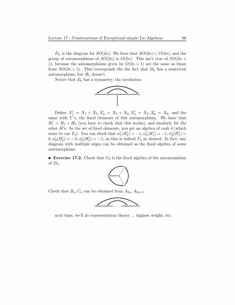
Lecture 17 - Constructions of Exceptional simple Lie Algebras 86
Dn is the diagram for SO(2n). We have that SO(2n) ⊂ O(2n), and thegroup of automorphisms of SO(2n) is O(2n). This isn’t true of SO(2n +1), because the automorphisms given by O(2n + 1) are the same as thosefrom SO(2n + 1). This corresponds the the fact that Dn has a nontrivialautomorphism, but Bn doesn’t.
Notice that E6 has a symmetry; the involution:
zz $$ !!
Define X ′1 = X1 + X5,X
′2 = X2 + X4,X
′3 = X3,X
′6 = X6, and the
same with Y ’s, the fixed elements of this automorphism. We have thatH ′
1 = H1 + H5 (you have to check that this works), and similarly for theother H’s. As the set of fixed elements, you get an algebra of rank 4 (whichmust be our F4). You can check that α′
1(H′2) = −1, α′
2(H′1) = −1, α′
3(H′1) =
0, α′3(H
′2) = −2, α′
2(H′3) = −1, so this is indeed F4 as desired. In fact, any
diagram with multiple edges can be obtained as the fixed algebra of someautomorphism:
Exercise 17.2. Check that G2 is the fixed algebra of the automorphismof D4:
11
111
00
ZZ
Check that Bn, Cn can be obtained from A2n, A2n+1
... zz $$ !!
next time, we’ll do representation theory ... highest weight, etc.

Lecture 18 - Representations 87
Lecture 18 - Representations
Representations
Let g be a semi-simple lie algebra over an algebraically closed field k ofcharacteristic 0. Consider the root decomposition g = h ⊕⊕α gα, and letV be a finite-dimensional representation of g. Because all elements of h aresemisimple, and because Jordan decomposition is preserved, the elements ofh can be simultaneously diagonalized. That is, we may write V =
⊕
µ∈h∗ Vµ,where Vµ = v ∈ V |hv = µ(h)v ∀h ∈ h. We call Vµ a weight space, and µthe weights. Define P (V ) = µ ∈ h∗|Vµ 6= 0. The multiplicity of a weightµ ∈ P (V ) is dimVµ, and is denoted mµ.
Example 18.1. You can take V = k (the trivial representation). ThenP (V ) = 0 and m0 = 1.
Example 18.2. If V = g and we take the adjoint representation, then wehave that P (V ) = ∆ ∪ 0, with mα = 1 for α ∈ ∆, and m0 = the rank ofg.
We can plot the set of weights in h∗:
Example 18.3. Let g = sl(3):
ε188ε2 ff
ε3
−ε1t| qqq
qqqqqqqqq
−ε2"*
MMMMMM
MMMMMM
−ε3KS
ε1 − ε2//
ε1 − ε3FF ε2 − ε1 oo
ε2 − ε3 XX1111111111
ε3 − ε1
ε3 − ε211
1111
1111
For the adjoint representation, the weights are shown in single lines.If E is the standard 3-dimensional representation, then we get weights
ε1, ε2, ε3, shown in dotted lines.We can also take the dual representation E∗. In general, the weights
of the dual representation are the negatives of the original representationbecause 〈hφ, v〉 = −〈φ, hv〉, so we get the double lines.
Note that the sum of these is a G2. (We noted earlier that G2 has somesl(3)s sitting around).
Properties: For V finite-dimensional
(1) µ(Hα) ∈ Z for any root α and µ ∈ P (V ).
This is because all weights of any representation of sl(2) are integers,so restricting to our little sl(2), we get this result.

Lecture 18 - Representations 88
(2) gαVµ ⊆ Vµ+α for α ∈ ∆, µ ∈ P (V ).
To check this:
h(xαv) = xαhv + [h, xα]v
= xαµ(h)v + α(h)xαv
= (µ+ α)(h)xαv
(3) If µ ∈ P (V ) and w ∈W , then w(µ) ∈ P (V ) and mµ = mw(µ).
To see this, it is sufficient to check for simple reflections w = ri. Recallthat for each reflection, there is a special element of the group G itself(coming from the small SL(2) ⊆ G). It is expXi exp(−Yi) expXisi ∈G. Then si(h) = h and si(Vµ) = Vriµ.
Example 18.4. If g = sl(3), then we get W = S3 = D3. The orbit of apoint can have a couple of different forms. If the point is on a mirror, thenyou get a triangle. For a generic point, you get a hexagon (which is notregular, but still symmetric).
It is pretty clear that knowing the weights and multiplicities gives us alot of information about the representation. However, it is hard to drawpictures in more than three dimensions, so instead you write the followingexpression:
chV =∑
µ∈P (V )
mµeµ
You can formally add and multiply these expressions: ch is additive withrespect to direct sum and multiplicative with respect to tensor products:
ch(V ⊕W ) = chV + chW
ch(V ⊗W ) = (chV )(chW )
This is because Vµ ⊗Wν ⊆ (V ⊗W )µ+ν . You can also check that the ch ofthe dual is
∑mµe
−µ. If you don’t care about multiplication, then you cando infinite-dimensional stuff.
Relations to group characters: if you have G → GL(V ), then we havethe characters χV (g) = trV (g). How are these related? Well, you canexponentiate h to get a subgroup H ⊆ G. To compute χV (exp h) for h ∈ h,you just need to add the exp’s of the eigenvalues of h:
χV (exph) = tr(exph) =∑
mµeµ(h).
Recall that group characters are constant on conjugacy classes. If youlook at different Cartan subalgebras, then something ... the character isdetermined by its values on the Cartan. . .This is a good way to keep trackof weights.
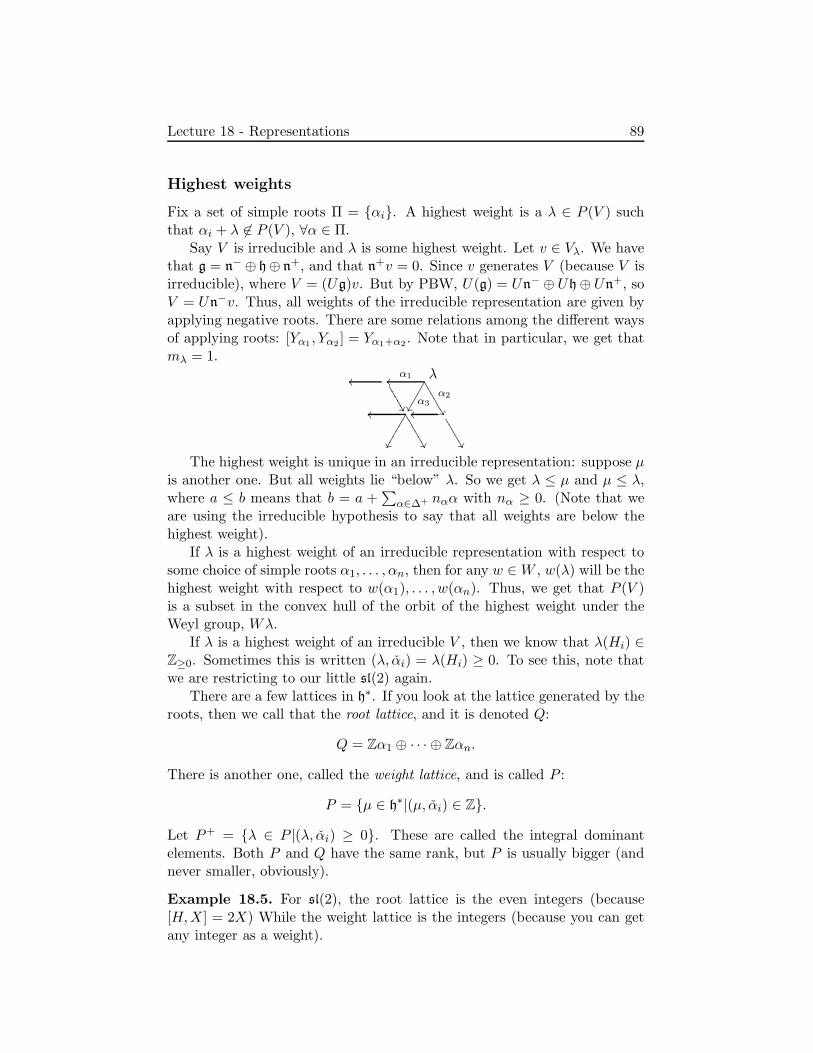
Lecture 18 - Representations 89
Highest weights
Fix a set of simple roots Π = αi. A highest weight is a λ ∈ P (V ) suchthat αi + λ 6∈ P (V ), ∀α ∈ Π.
Say V is irreducible and λ is some highest weight. Let v ∈ Vλ. We havethat g = n− ⊕ h⊕ n+, and that n+v = 0. Since v generates V (because V isirreducible), where V = (Ug)v. But by PBW, U(g) = Un− ⊕ Uh⊕ Un+, soV = Un−v. Thus, all weights of the irreducible representation are given byapplying negative roots. There are some relations among the different waysof applying roots: [Yα1 , Yα2 ] = Yα1+α2 . Note that in particular, we get thatmλ = 1.
λα1oo
α2
11
1111
α3
oo
11
111
oo
11
111oo
11
1111
The highest weight is unique in an irreducible representation: suppose µis another one. But all weights lie “below” λ. So we get λ ≤ µ and µ ≤ λ,where a ≤ b means that b = a +
∑
α∈∆+ nαα with nα ≥ 0. (Note that weare using the irreducible hypothesis to say that all weights are below thehighest weight).
If λ is a highest weight of an irreducible representation with respect tosome choice of simple roots α1, . . . , αn, then for any w ∈W , w(λ) will be thehighest weight with respect to w(α1), . . . , w(αn). Thus, we get that P (V )is a subset in the convex hull of the orbit of the highest weight under theWeyl group, Wλ.
If λ is a highest weight of an irreducible V , then we know that λ(Hi) ∈Z≥0. Sometimes this is written (λ, αi) = λ(Hi) ≥ 0. To see this, note thatwe are restricting to our little sl(2) again.
There are a few lattices in h∗. If you look at the lattice generated by theroots, then we call that the root lattice, and it is denoted Q:
Q = Zα1 ⊕ · · · ⊕ Zαn.
There is another one, called the weight lattice, and is called P :
P = µ ∈ h∗|(µ, αi) ∈ Z.
Let P+ = λ ∈ P |(λ, αi) ≥ 0. These are called the integral dominantelements. Both P and Q have the same rank, but P is usually bigger (andnever smaller, obviously).
Example 18.5. For sl(2), the root lattice is the even integers (because[H,X] = 2X) While the weight lattice is the integers (because you can getany integer as a weight).

Lecture 18 - Representations 90
Thus, you can look at P/Q, which is the center of the simply connectedgroup corresponding to g.
We have said that the highest weight is in P+.
Exercise 18.1. Show that P+ is the fundamental domain of theW actionon P . (This follows from the fact that W acts simply and transitively onthe set of bases).
In the case of sl(3), we get:
•••••
•••••
••••••
•••••
••••••
•••••
rr
rr
rr
rr
rr
rr
r
P+
α1
//
α2XX11111
For every µ ∈ P , there is a unique element w ∈W such that wµ ∈ P+.
Theorem 18.6. There is a bijection between P+ and the set of (isomor-phism classes of) finite-dimensional irreducible representations of g.
If you have an irreducible representation V , then to it we associate itshighest weight in P+. We already know that the map is well-defined (be-cause the highest weights are unique). For injectivity we must show thattwo different representations cannot have the same highest weight. For sur-jectivity, we need to show that every element of P+ is the highest weight ofsome irreducible representations.
We are going to use Verma modules because they are nice. A lot ofpeople avoid using them, but I don’t think that is a good approach.
Let V be our representation with highest weight λ. That means that Vλis a 1-dimensional representation of the subalgebra b = h⊕n+ ⊆ g. There isan embedding Vλ → V , which is a homomorphism of Ub-modules (that is,of representations of b). Thus, there is an induced object U(g)⊗Ub Vλ, andthere is a homomorphism of Ug-modules from U(g)⊗Ub Vλ to V . However,there is a problem: when we do the induction, we get something infinitedimensional.
Definition 18.7. A Verma module is M(λ) = Ug ⊗Ub Vλ.
Verma Modules are universal in the sense that all representations withhighest weight λ are quotients of M(λ). To understand what M(λ) is as avector space, we use PBW to get that Ug = Un− ⊗ Uh ⊗ Un+ = U(n−) ⊗Ub (these tensor products are as vector spaces). Thus, we get M(λ) =

Lecture 18 - Representations 91
Un− ⊗k Vλ. The Verma module is something universal ... . We can choosea basis U(n−), say α1, . . . , αn, αn+1, . . . , αN (the positive roots, ordered).Then Yαii≤N is a basis for n−, and by PBW Y k1
α1· · ·Y kN
αNv is a basis in
U(n−)⊗k Vλ M(λ). Even though the Verma module is infinite-dimensional,it still has a weight decomposition:
h(Y k1α1
· · ·Y kNαNv) = (λ− k1α1 − · · · )(h)(Y k1
α1· · ·Y kN
αNv)
11
1
111
2
2
1112
3
1 1
1
1 111
1
2
1111
2
12 1
2
1
2
111
12
2
3
111
23
1
2
3 1
1111
12
1111
1 '!&"%#$3
1111
1
All the multiplicities along the edges are 1. Then you get multiplicity2 just below λ because there is a linear dependence. You can check thatparallel to the edges, you keep getting multiplicity 2. And in general, themultiplicity grows by 1 with every step you take from the wall.
Exercise 18.2. Check this out.
We have a nice formula:
mµ = #λ− µ =∑
α∈∆+
kαα
This is called the Kostant partition function.Let’s calculate the multiplicity circled in the previous picture. We have
that 2α3 = α3 + α2 + α1 = 2α1 + 2α2, so the multiplicity is 3. Thesecalculations will prepare you for the Weyl formula.
Claim. A Verma module M(λ) has a unique proper maximal submoduleN(λ).
Proof. N being proper is equivalent to N ∩ Vλ = 0. This property is clearlypreserved under taking sums, so you get a unique maximal submodule.
If V and W are irreducible representations that have the same highestweight, then they are both the unique irreducible quotient M(λ)/N(λ), sothey are isomorphic. Thus, the map from irreducibles to P+ is injective.
Now we need to show that if λ ∈ P+, then the quotient M(λ)/N(λ) isfinite-dimensional. The trick is to look at sl(2). The picture of the Vermamodule is that you have all the weights λ − kα with multiplicity 1. If youmod out by any submodule, you get something finite-dimensional.
Lecture 18 - Representations 92
Sketch of Proof. If w is a weight vector in a Verma module such that Xiw =0 for i = 1, . . . , n, then we claim that w ∈ N(λ). To see this, you note thatyou can never get back to λ.
Suppose 〈λ, αi〉 = ni ∈ Z≥0. Then w = Y ni+1i v and Xiw = 0. We have
XjYni+1v = Y ni+1
i Xjv = 0 because [Xj , Yi] = 0 for i 6= j.Consider the quotient M(λ)/N(λ) = V (λ). Then we have that Y ni+1
i v =0, so the Yi act locally nilpotently on V (λ). And Xi also act locally nilpo-tently (even on the Verma module, not just the quotient). Then si =expXi exp(−Yi) expXi, and we get that P (V (λ)) is W invariant because ofsomething. But then you can start with λ and look at the orbit. The weightsare in the convex hull, which is bounded, so V (λ) is finite-dimensional.
We introduced these Verma modules because we will use them later towrite down the character formula.
Next time:
(1) Fundamental representations, etc.
(2) Weyl character formula

Lecture 19 - The Weyl character formula 93
Lecture 19 - The Weyl character formula
If λ ∈ P+ (i.e. (λ, αi) ∈ Z≥0 for all i), then we can construct a representationV (λ) which is a representation with λ as the highest weight. We define thefundamental weights ω1, . . . , ωn of a representation to be those weights forwhich (ωi, αj) = δij . It is clear that any weight λ = λ1ω1 + · · · + λnωn forλi ≥ 0. So people often draw the Dynkin diagrams with the fundamentalweights labelled:
1 0 ... 0 0 This is V (ω1), the first fundamental representation for sl(n). Here is theadjoint representation:
1 0 ... 0 1 Observe that if v ∈ V a highest vector, and w ∈ W another highest weightvector in another representation, then v ⊗ w ∈ V ⊗W is a highest weightvector. It follows that every finite dimensional irreducible representationcan be realized as a subrepresentation in a tensor product of fundamentalrepresentations.
Example 19.1. Let’s calculate the fundamental weights for sl(n+1). RecallFundamentalweights ofsl(n+ 1)that we have simple roots ε1 − ε2, . . . , εn− εn+1, which are also the coroots.
It follows that ωi = ε1 + · · · + εi for i = 1, . . . , n.Consider ΛkE, where E is the standard representation. Let e1, . . . , en+1
be a weight basis for E (i.e. the vectors e1, . . . , en are a basis, with decreasingweights ε1, . . . , εn). We’d like to write down the weights P (ΛkE). Note thatΛkE is spanned by the vectors ei1∧· · ·∧eik , which have weights εi1 +· · ·+εik .Thus, the highest weight is ε1+· · ·+εk = ωk, so ΛkE = Vωk
is a fundamentalrepresentation. Notes also that the weights form the single orbit Wωk.Representations where the weights form a single orbit are called minuscule.ΛkE = Vωk
Remark 19.2. If λ is the highest weight of the representation V , then −λ isa weight of V ∗. To compute the highest weight of V ∗, we need to get back
Highestweights ofdualsinto P+, so we apply the longest word in the Weyl group: −w(λ) is the
highest weight of V ∗. Thus, there is a fixed involution of the Weyl chamber(namely, −w) which takes the highest weight of V to the highest weight ofV ∗. It is clear that −w preserves the set of simple roots and preserves innerproducts, so it is an involution of the Dynkin diagram.
In the case of sl(n + 1), the involution is ... ss ++ss ++ . Inparticular, the dual of the standard representation Vω1 is Vωn .
The bijection between P+ and irreducible representations implies
Corollary 19.3. If V,W are finite dimensional representations, with chV =chW , then V ≃W .
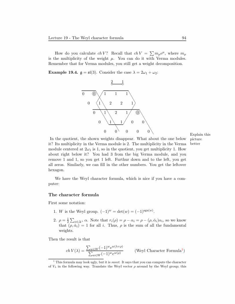
Lecture 19 - The Weyl character formula 94
How do you calculate chV ? Recall that chV =∑mµe
µ, where mµ
is the multiplicity of the weight µ. You can do it with Verma modules.Remember that for Verma modules, you still get a weight decomposition.
Example 19.4. g = sl(3). Consider the case λ = 2ω1 + ω2:
2 1
1
1
0 '!&"%#$
0
0
1
2
1
0
0
1
2
2
1
0
0 '!&"%#$
1
1
1
0
0
0
0
0
0
11111111
1111
1111
1111
11
1111
1111
1111
1111
1111
1111
1
1111
1111
1111
111
In the quotient, the shown weights disappear. What about the one belowExplain thispicturebetterit? Its multiplicity in the Verma module is 2. The multiplicity in the Verma
module centered at 2ω1 is 1, so in the quotient, you get multiplicity 1. Howabout right below it? You had 3 from the big Verma module, and youremove 1 and 1, so you get 1 left. Furthur down and to the left, you getall zeros. Similarly, we can fill in the other numbers. You get the leftoverhexagon.
We have the Weyl character formula, which is nice if you have a com-puter:
The character formula
First some notation:
1. W is the Weyl group. (−1)w = det(w) = (−1)sgn(w).
2. ρ = 12
∑
α∈∆+ α. Note that ri(ρ) = ρ− αi = ρ− (ρ, αi)αi, so we knowthat (ρ, αi) = 1 for all i. Thus, ρ is the sum of all the fundamentalweights.
Then the result is that
chV (λ) =
∑
w∈W (−1)wew(λ+ρ)
∑
w∈W (−1)wew(ρ)(Weyl Character Formula1)
1 This formula may look ugly, but it is sweet. It says that you can compute the characterof Vλ in the following way. Translate the Weyl vector ρ around by the Weyl group; this

Lecture 19 - The Weyl character formula 95
note that the numerator and denominator is skew with respect to the actionof W , so ch is W -symmetric. The denominator is called the Weyl denomi-nator.
For those who know something about the representation theory of gl(n),I’d like to show the connection between these two things. If g = gl(n) ⊃sl(n). Let zi = eεi , so z1 · · · zn = 1. We know that W ≃ Sn, which acts onthe zi by permutation. We have that
ρ =1
2
∑
i<j
εi − εj
=1
2((n − 1)ε1 + (n− 3)ε2 + · · · + (1 − n)εn)
=
soeρ = zn−1
1 zn−32 · · · z1−n
n .
Then
chV (λ) =
∑
σ∈Sn(−1)σza1+n−1
σ(1) · · · zan
σ(n)∑
σ∈Sn(−1)σzn−1
σ(1) · · · z0σ(n)
The denominator (call it D) is the famous Vandermonde determinant, whichyou should know
vandermondeWhere λ = a1ε1 + · · · + anεn. Then (λ, αi) = ai − aa+1 ≥ 0.Usually, the representations are encoded as Young diagrams. The marks
on the dynkin diagram are the differences in consecutive rows in the youngdiagram.
The numerator is
Dλ = det
za1+n−11 . . . za1+n−1
n...zan1
will form some polytope. Make a piece of cardboard shaped like this polytope (ok, somaybe this is only practical for rank 2), and put (−1)w at the vertex w(ρ). This is yourcardboard denominator. Now the formula tells you that when you center your cardboarddenominator around any weight, and then add the multiplicities of the weights of Vλ atthe vertices with the appropriate sign, you’ll get zero (unless you centered your cardboardat w(λ + ρ), in which case only one non-zero multiplicity shows up in the sum, so you’llget ±1). Since we know that the highest weight has multiplicity 1,we can use this to compute the rest of the character.For sl(3), your cardboard denominator will be a hexagon, and onestep of computing the character of V2ω1+ω2
might look like:0 = 0 − 1+ ? − 1 + 0 − 0, so ? = 2. Since ch V is symmetric withrespect to W , all three of the ?s must be 2.
0
0
0
1
1
1
?
1
1
?
?
1
1
1
1
11
11
Lecture 19 - The Weyl character formula 96
So the character is the Schur polynomial.
Proof of character formula. Express chV (λ) as a linear combination of char-acters of Verma modules. This is what we did with the picture for sl(3).
Consider sl(2). We know what the representations are: V (n).The Verma module is infinite in the negative direction, but at−n − 2, there is another Verma module, which is also infinite.We have that ρ = ω = α
2
picture
Thus, we claim that chV (n) = chM(n)− chM(−n− 2). To seethis, we compute chM(n) = enω + e(n−2)ω + · · · = enω(1+ e−α+
e−2α + · · · ) = enω
1−e−α , and similarly, chM(−n − 2) = e(−n−2)ω
1−e−α .
So we get that chM(n) = e(n+1)ω
(eα/2−e−α/2)and chM(−n − 2) =
e−(n+1)ω
(eα/2−e−α/2)
So we have that chV (λ) = e(n+1)ω−e(−n−1)ω
eα/2−e−α/2
Consider M(λ) for λ ∈ P . Then
chM(λ) = eλ∏
α∈∆+
(1 + e−α + e−2α + · · · )
wheremµ = #λ− µ =
∑
α∈∆+
nαα
We claim that this character is
∏
α∈∆+
(1 + e−α + · · · ) =∑
mγeγ
where mγ = #γ =∑nαα. Thus, we have that
chM(λ) =eλ
∏
α∈∆+(1 − e−α)=
eλ+ρ
∏
α∈∆+(eα/2 − e−α/2)1
where ρ = 12
∑
α∈∆+ α.Now recall the Casimir operator. If ei is a basis for g, with dual basis
fi. Then the Casimir operator is Ω =∑eifi ∈ Ug. We showed before
that Ω is in the center of Ug, so that Ωg = gΩ for all g ∈ g.
Claim. Ω|M(λ) = (λ+ 2ρ, λ)Id2. This is 2

Lecture 19 - The Weyl character formula 97
We will use the identity (λ+ 2ρ, λ) = (λ+ ρ, λ+ ρ)− (ρ, ρ). It is enoughto show that something highest weight, then use stuff
Let ui be an orthonormal basis for h. Xαα∈∆,
Yα(Xα,Yα)
dual basis.
We can write
Ω =
n∑
i=1
u2i +
∑
α∈∆+
XαYα(Xα, Yα)
+YαXα
(Xα, Yα)
Let v be the highest vector. then we have that
Ωv = (
n∑
1
λ(ui)2)v +
∑
α∈∆+
λ(Hλ)
(Xα, Yα))
since ui(v) = λ(ui)v, Xαv = 0, YαXαv = 0, XαYα = Hα + YαXα, XαYαv =λ(Hα)v.
We have that λ(Hα) = 2(λ,α)(α,α) and (Xα, Yα) = 1
2(Hα,Hα) = 2(α,α) .
We get that
Ωv = (λ, λ)v +∑
α∈∆+
(λ, α)v = what we want
Remark 19.5. Let
Ωλ = µ ∈ P |(λ+ ρ, λ+ ρ) = (µ+ ρ, µ+ ρ)
geometrically, this is a sphere centered somewhere. This is a finite set. Thisis 3.
We have that M(λ) has a unique irreducible quotient, which we denoteV (λ). If λ ∈ P+, then this is finite-dimensional, but in general, it is not.For example, sometimes the Verma module itself is irreducible (like in thesl(2) case).
Point number 4 is that there exists a finite filtration of the Verma module
0 = F0M(λ) ⊂ F1M(λ) ⊂ · · · ⊂ FkM(λ) = M(λ)
such that the consecutive quotients are irreducible with Fi/Fi−1 ≃ V (µ) forsome µ ∈ Ωλ.
We say that a vector w is singular of weight µ if hw = µ(h)w andn+w = 0.
Suppose a module is generated by some highest vector, and all singularvectors are proportional to the highest vector, then the representation is
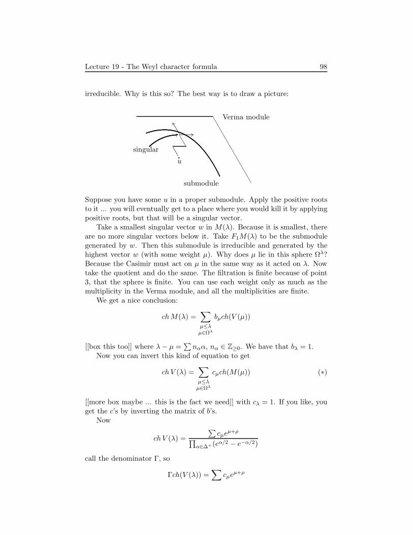
Lecture 19 - The Weyl character formula 98
irreducible. Why is this so? The best way is to draw a picture:
Verma module
1111
1111
1111
1111
1111
111
submodule
u·1111
1111
XX
//
singular
00
Suppose you have some u in a proper submodule. Apply the positive rootsto it ... you will eventually get to a place where you would kill it by applyingpositive roots, but that will be a singular vector.
Take a smallest singular vector w in M(λ). Because it is smallest, thereare no more singular vectors below it. Take F1M(λ) to be the submodulegenerated by w. Then this submodule is irreducible and generated by thehighest vector w (with some weight µ). Why does µ lie in this sphere Ωλ?Because the Casimir must act on µ in the same way as it acted on λ. Nowtake the quotient and do the same. The filtration is finite because of point3, that the sphere is finite. You can use each weight only as much as themultiplicity in the Verma module, and all the multiplicities are finite.
We get a nice conclusion:
chM(λ) =∑
µ≤λµ∈Ωλ
bµch(V (µ))
[[box this too]] where λ− µ =∑nαα, nα ∈ Z≥0. We have that bλ = 1.
Now you can invert this kind of equation to get
chV (λ) =∑
µ≤λµ∈Ωλ
cµch(M(µ)) (∗)
[[more box maybe ... this is the fact we need]] with cλ = 1. If you like, youget the c’s by inverting the matrix of b’s.
Now
chV (λ) =
∑cµe
µ+ρ
∏
α∈∆+(eα/2 − e−α/2)
call the denominator Γ, so
Γch(V (λ)) =∑
cµeµ+ρ
Lecture 19 - The Weyl character formula 99
You have an action of W on the LHS. You can check that w(Γ) = (−1)wΓ,so the RHS must also be skew-symmetric with respect to the action of W .Because of this, you can combine the terms by orbits of the Weyl group
Try to finish this yourself. Calculate the cµ.
Next time, we’ll finish, and talk about the relation to compact groups.

Lecture 20 100
Lecture 20
This is Serganova’s last lecture.We have that
chV (λ) =∑
µ≤λcλ=1
cµchM(µ) (∗)
which we get from
chM(λ) =∑
µ≤λbλ=1
chV (µ)
where µ ∈ P , but not in P+. The bµ are Kazhdan-Lusztig multiplicities,and are hard to compute. But we can compute the cµ when λ ∈ P+.
There was once a conjecture that all the cµ were ±1, but this is false,and leads to some interesting stuff.
Since we know the characters of all the Verma modules, we can rewrite(∗) as
∏
α∈∆+
(eα/2 − e−α/2)chV (λ) =∑
µ∈Ωλ,µ≤λcµe
µ+λ
we know that w(LHS) = (−1)wLHS, so the same must be true of the RHS:
w(∑
cµeµ+ρ) = (−1)w
∑
cµeµ+ρ
This is equivalent to saying that cw(µ+ρ)−ρ = (−1)wcµ. We also knowthat cλ = 1, so you get
∑
(−1)wew(λ+ρ) +∑
µ<λµ+ρ∈P+
(∑
w∈W(−1)wew(µ+ρ))
W acts in such a way that every orbit contains an element of P+, so we cantake µ+ ρ ∈ P+. We want to show that cµ = 0 for µ < λ. µ ∈ Ωλ. We havethat (µ+ ρ, µ+ ρ) = (λ+ ρ, λ+ ρ) and
λ− µ =∑
niαi
with ni ∈ Z≥0. So we get that (λ−µ, λ+µ+2ρ) = 0, so (∑niαi, λ+µ+2ρ) =
0, so for λ+ µ+ ρ ∈ P+, we have that
(λ+ µ+ ρ, αi) ≥ 0
(ρ, αi) > 0, recall that (ρ, αi) = 1.
∏
α∈∆+
(eα/2 − e−α/2)chV (λ) =∑
w∈W(−1)wew(λ+ρ)
Lecture 20 101
λ = 0, chV (0) = e0 = 1. gives the Weyl denominator identity:∏
α∈∆+
(eα/2 − e−α/2) =∑
w∈W(−1)wew(ρ) = D
So we get the formula
chV (λ) =1
D∑
w∈W(−1)wew(λ+ρ)
Dimension formula: we can get
dimV (λ) =∏
α∈∆+
(λ+ ρ, α)
(ρ, α)
In the sl(n) case, you get ε1 + · · · + εn = 0, and you get ρ = stuff , soyou can compute dimension as
∏
α∈∆+
(ρ, α) = (n− 1)!(n − 2)! · · · = (n− 1)!!
If λ =∑aiεi, then we get
∏
i<j
(ai + aj + j − i)
We can prove this from the character formula? We have to take a limit ase→ 1 (since we get 0/0 if we take e = 1).
limu→0
∑(−1)we(w(λ+ρ),u)
∑(−1)we(w(ρ),u)
Let u = ρt for t→ 0, then we get∏
α∈∆+ et(λ+ρ,α/2) − e−t(λ+ρ,α/2)
∏
α∈∆+ et(ρ,α/2) − e−t(ρ,α/2)
using (w(λ+ ρ), u) = (λ+ ρ,w−1(u)), and from here it is just an exercise inL’hopital.
You can keep playing with this formula to get some nice things. It isnice for calculating V (λ) ⊗ V (µ) =
∑bνλµV (ν). As for finite groups, we do
this by looking that chV (λ) · chV (µ) and writing it as∑bνλµchV (ν). In
the finite group case, we used orthogonality relations among the characters.We have a natural inner product 〈eλ, eµ〉 = δλ+µ,0, but this isn’t good
for some reason. The inner product we use is
(φ,ψ) =1
|W |(Dφ, Dψ)
where eλ = e−λ. It is a calculation to check that characters of irreduciblerepresentations form an orthonormal basis with respect to this inner prod-uct.

Lecture 20 102
Compact Groups
So far we classified semi-simple Lie algebras over a characteristic 0 alge-braically closed field. How is this connected to compact groups. Let G be acompact connected group (over R), like SU(2), which is topologically S3.
SU(n) = X ∈ GL(n,C)|XtX = Id, detX = 1
Exercise 20.1. If G is abelian, then it is a product of circles, so it is Tn.
There exists the G-invariant volume form satisfying
(1)∫
G ω = 1
(2)∫
G f(gh)ω =∫
G f(hg)ω =∫
G f(g)ω
It is a nice exercise to construct this ... you take a volume near the identityand translate it around. So you pick ωe ∈ Λtop(TeG)∗ and define ωg =L∗g−1ωe. Check for yourself that this form is right invariant.
From this you get a nice theorem:
Theorem 20.1. If V is a finite dimensional representation of G (overR), then there exists a positive definite G-invariant inner product on V :(gv, gw) = (v,w).
Proof. Start with some positive definite inner product Q(v,w), and define
(v,w) =
∫
GQ(gv, gw)ω
which is invariant.
It follows that any finite dimensional representation of a compact groupG is completely reducible (i.e. splits into a direct sum of irreducibles). Bythe way, representations of Lie groups are always taken to be smooth.
In particular, look at Ad : G → GL(g), which gives ad : g → gl(g),which must split into irreducible ideals: g = g1 ⊕ · · · gk ⊕ a, each of which isone-dimensional or simple (dump all the one-dimensional guys into a, whichis then the center). Thus, the Lie algebra of a compact group is the directsum of its center and a semi-simple Lie algebra. Such a Lie algebra is calledreductive.
If G is simply connected, then I claim that a is trivial. This is becausethe simply connected group connected to a must be a torus, so a centergives you some fundamental group. Thus, if G is simply connected, then g
is semi-simple.Criterion: If the Killing form B on g is negative definite, then the cor-
responding group is compact.

Lecture 20 103
If you have g → gl(g), and you know that g has an invariant positivedefinite product, so it lies in so(g). Here you have At = −A, so you have tocheck that tr(A2) < 0. It is not hard to check that the eigenvalues of A areimaginary (as soon as At = −A), so we have that the trace of the square isnegative.
g is a Lie algebra over RHow to classify compact Lie algebras? We know the classification over
C, so we can always take g gC = g ⊗R C, which remains semi-simple.However, this process might not be injective. For example, take su(2) =(a b−b a
)|a ∈ Ri, b ∈ C and sl(2,R), then they complexify to the same
thing.g in this case is called a real form of gC. So you can start with gC and
classify all real forms.
Theorem 20.2 (Cartan?). Every semi-simple Lie algebra has exactly one(up to isomorphism) compact real form.
For example, for sl(2) it is su(2).Classical Lie groups: SL(n,C), SO(n,C) (SO has lots of real forms of
this, because in the real case, you get a signiture of a form; in the complexcase, all forms are isomorphic), Sp(2n,C). What are the correspondingcompact simple Lie groups?
Compact real forms: SU(n) = the group of linear operators on Cn pre-serving a positive definite Hermitian form. SL(n) = the group of linearoperators on Rn preserving a positive definite symmetric bilinear form.Sp(2n) =the group of linear operators on Hn preserving a positive definiteHermitian form
We’re not going to prove this theorem because we don’t have time, butlet’s show existence.
Proof of existence. Suppose gC = g ⊗R C = g ⊕ ig. Then you can constructσ : gC → gC “complex conjugation”. Then σ preserves the commutator,but it is an anti-linear involution. Classifying real forms amounts to clas-sifying all anti-linear involutions. There should be one that correspondsto the compact algebra. Take X1, . . . ,Xn,H1, . . . ,Hn, Y1, . . . , Yn genera-tors for the algebra. Then we just need to define σ on the generators:σ(Xi) = −Yi, σ(Yi) = −Xi, σ(Hi) = −Hi, and extend anti-linearly. Thisparticular σ is called the Cartan involution.
Now we claim that g = (gC)σ = X|σ(X) = X is a compact simple Liealgebra. We just have to check that the Killing form is negative definite. Ifyou take h ∈ h, written as h =
∑aiHi, then σ(h) = h implies that all the ai
are purely imaginary. This implies that the eigenvalues of h are imaginary,which implies that B(h, h) < 0. You also have to check it on Xi, Yi. The
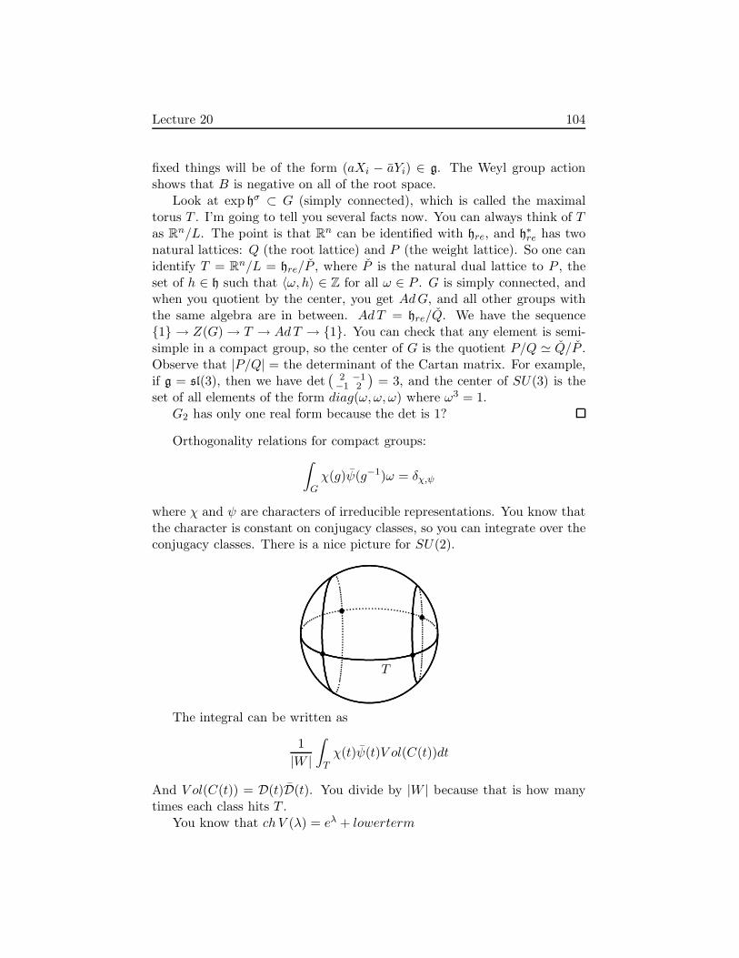
Lecture 20 104
fixed things will be of the form (aXi − aYi) ∈ g. The Weyl group actionshows that B is negative on all of the root space.
Look at exp hσ ⊂ G (simply connected), which is called the maximaltorus T . I’m going to tell you several facts now. You can always think of Tas Rn/L. The point is that Rn can be identified with hre, and h∗re has twonatural lattices: Q (the root lattice) and P (the weight lattice). So one canidentify T = Rn/L = hre/P , where P is the natural dual lattice to P , theset of h ∈ h such that 〈ω, h〉 ∈ Z for all ω ∈ P . G is simply connected, andwhen you quotient by the center, you get AdG, and all other groups withthe same algebra are in between. AdT = hre/Q. We have the sequence1 → Z(G) → T → AdT → 1. You can check that any element is semi-simple in a compact group, so the center of G is the quotient P/Q ≃ Q/P .Observe that |P/Q| = the determinant of the Cartan matrix. For example,if g = sl(3), then we have det
(2 −1−1 2
)= 3, and the center of SU(3) is the
set of all elements of the form diag(ω, ω, ω) where ω3 = 1.G2 has only one real form because the det is 1?
Orthogonality relations for compact groups:
∫
Gχ(g)ψ(g−1)ω = δχ,ψ
where χ and ψ are characters of irreducible representations. You know thatthe character is constant on conjugacy classes, so you can integrate over theconjugacy classes. There is a nice picture for SU(2).
T
•
••
•
The integral can be written as
1
|W |
∫
Tχ(t)ψ(t)V ol(C(t))dt
And V ol(C(t)) = D(t)D(t). You divide by |W | because that is how manytimes each class hits T .
You know that chV (λ) = eλ + lowerterm

Lecture 21 105
Lecture 21
The new lecturer is Borcherds.This is the last third of the course: Examples and calculations. The
(unofficial) goal is to prove no theorems. We’ll try to do
1. Clifford algebras and spin groups.
2. Construction of all Lie groups and all representations. You mightsay this is impossible, so let’s just try to do all simple ones, and inparticular E8, E7, E6.
3. Representations of SL2(R).
Today we’ll give an overview of Lie algebras and Lie groups. We’ll com-pare with algebraic groups (matrix groups), and finite groups.
What does a general Lie group look like?
Example 21.1. Let G be the group of all shape-preserving (translations,rotations, reflections, dilations) transformations of R4, sometimes calledR4 · GO4(R).1 The is pretty much the smallest possible Lie group withall the properties of a general Lie group.
(1) G has a connected component Gconn, which is a normal subgroup, andG/Gconn is a discrete group.
Any Lie group can be built from a connected Lie group and a discretegroup (0-dimensional group). Classifying discrete groups is completelyhopeless.
(2) We let Gsol be the maximal normal connected solvable subgroup ofGconn. Recall that solvable means that there is a chain Gsol ⊇ G′
sol ⊇· · · ⊃ 1 where all consecutive quotients are abelian. So you buildsolvable groups out of abelian groups.
Gconn/Gsol is connected and has no solvable normal subgroups. Itturns out that it is much easier to deal with the group if you kill offall the solvable subgroups like this. Groups like this are semi-simple.They are almost a product of simple groups. A semi-simple group Gmodulo its discrete center is a product of simple groups.
The nice thing is that connected simple Lie groups are all completelyclassified. The list is quite long, and it has a lot of infinite seriesand a lot of exceptional guys. Some examples are PSU(n), PSLn(R),PSLn(C). You can go from simple Lie groups to simple Lie algebras
1R4 is translations, G is multiplication by scalers, O is reflections and rotations

Lecture 21 106
over R, then complexify to get Lie algebras over C. This last step isfinite-to-one, and they can be classified fairly easily. For example, theLie algebras of sl2(R) and su2(R) are different, but they have the samecomplexification, sl2(C), which, by the way, is actually simple as a realLie algebra. Its complexification is not simple, it is sl2(C) ⊕ sl2(C).
Suppose Gsol is solvable. The only thing you can say is that its derivedsubgroup G′
sol is nilpotent. That is, G′ ⊇ [G′, G′] ⊇ [G′, [G′, G′]] ⊇· · · ⊇ 1, or rather there is a chain such that Gi/Gi+1 ⊆ the center ofG1/Gi+1. Thus, nilpotent groups can be built up by taking centralextensions. Nilpotent groups are in practice not classifiable. The sim-ply connected ones are all isomorphic to subgroups of upper-triangularmatrices
1 ∗. . .
10 1
If you put arbitrary things on the diagonal, that is what the solvablegroups look like.
We have the picture
G
Gconn
G∗
Gsol
Gnil
1
discrete; classification hopeless
∏ simples; classified
abelian discrete
abelian
classification trivial
nilpotent; classification a mess
all connected
In our case, G is R4 · GO4(R). The connected component Gconn isR4 · GO+
4 (R), which is the stuff that preserves orientation. Gsol is R4 · R+
(rescaling). Gnil is R4. Gconn/Gsol is SO4(R), Gsol/Gnil is R+. Gconn/G∗ isPSO4(R) ≃ SO3(R) × SO3(R). G∗/Gsol is Z/2Z.
Note: What is O4(R)? It almost is the product O3(R) × O3(R). Tosee this is to look at the quaternions H, which is an associative, but notcommutative algebra. Notice that qq = a2 + b2 + c2 + d2, which is > 0 ifq 6= 0, so any non-zero quaternion has an inverse. Thus, H is a divisionalgebra. Put R4 to be the quaternions, and S3 is the unit sphere in this R4
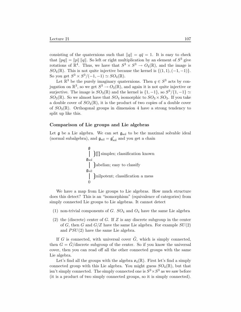
Lecture 21 107
consisting of the quaternions such that ‖q‖ = qq = 1. It is easy to checkthat ‖pq‖ = ‖p‖ ‖q‖. So left or right multiplication by an element of S3 giverotations of R4. Thus, we have that S3 × S3 → O4(R), and the image isSO4(R). This is not quite injective because the kernel is (1, 1), (−1,−1).So you get S3 × S3/(−1,−1) ≃ SO4(R).
Let R3 be the purely imaginary quaternions. Then q ∈ S3 acts by con-jugation on R3, so we get S3 → O3(R), and again it is not quite injective orsurjective. The image is SO3(R) and the kernel is 1,−1, so S3/1,−1 ≃SO3(R). So we almost have that SO4 isomorphic to SO3×SO3. If you takea double cover of SO4(R), it is the product of two copies of a double coverof SO3(R). Orthogonal groups in dimension 4 have a strong tendency tosplit up like this.
Comparison of Lie groups and Lie algebras
Let g be a Lie algebra. We can set gsol to be the maximal solvable ideal(normal subalgebra), and gnil = g′sol and you get a chain
g
gsol
gnil
0
∏ simples; classification known
abelian; easy to classify
nilpotent; classification a mess
We have a map from Lie groups to Lie algebras. How much structuredoes this detect? This is an “isomorphism” (equivalence of categories) fromsimply connected Lie groups to Lie algebras. It cannot detect
(1) non-trivial components of G. SO4 and O4 have the same Lie algebra
(2) the (discrete) center of G. If Z is any discrete subgroup in the centerof G, then G and G/Z have the same Lie algebra. For example SU(2)and PSU(2) have the same Lie algebra.
If G is connected, with universal cover G, which is simply connected,then G = G/discrete subgroup of the center. So if you know the universalcover, then you can read off all the other connected groups with the sameLie algebra.
Let’s find all the groups with the algebra o4(R). First let’s find a simplyconnected group with this Lie algebra. You might guess SO4(R), but thatisn’t simply connected. The simply connected one is S3×S3 as we saw before(it is a product of two simply connected groups, so it is simply connected).
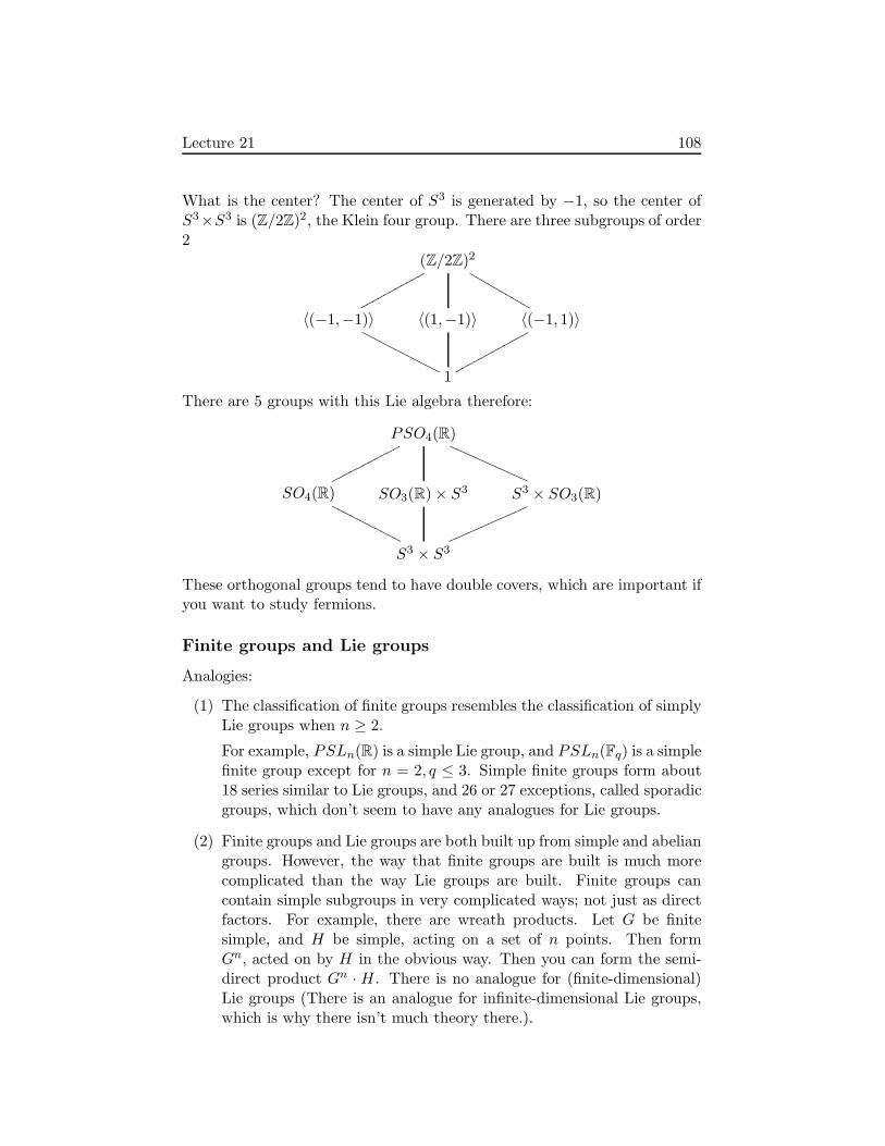
Lecture 21 108
What is the center? The center of S3 is generated by −1, so the center ofS3×S3 is (Z/2Z)2, the Klein four group. There are three subgroups of order2
(Z/2Z)2
qqqqqqqqqqq
LLLLLLLLLL
〈(−1,−1)〉
OOOOOOOOOOOO〈(1,−1)〉 〈(−1, 1)〉
qqqqqqqqqqqq
1
There are 5 groups with this Lie algebra therefore:
PSO4(R)
ppppppppppp
QQQQQQQQQQQQ
SO4(R)
OOOOOOOOOOOSO3(R) × S3 S3 × SO3(R)
mmmmmmmmmmmm
S3 × S3
These orthogonal groups tend to have double covers, which are important ifyou want to study fermions.
Finite groups and Lie groups
Analogies:
(1) The classification of finite groups resembles the classification of simplyLie groups when n ≥ 2.
For example, PSLn(R) is a simple Lie group, and PSLn(Fq) is a simplefinite group except for n = 2, q ≤ 3. Simple finite groups form about18 series similar to Lie groups, and 26 or 27 exceptions, called sporadicgroups, which don’t seem to have any analogues for Lie groups.
(2) Finite groups and Lie groups are both built up from simple and abeliangroups. However, the way that finite groups are built is much morecomplicated than the way Lie groups are built. Finite groups cancontain simple subgroups in very complicated ways; not just as directfactors. For example, there are wreath products. Let G be finitesimple, and H be simple, acting on a set of n points. Then formGn, acted on by H in the obvious way. Then you can form the semi-direct product Gn · H. There is no analogue for (finite-dimensional)Lie groups (There is an analogue for infinite-dimensional Lie groups,which is why there isn’t much theory there.).

Lecture 21 109
(3) Solvable finite groups need not have nilpotent group as a derived sub-group. Example: S4, with derived group A4, which is not nilpotent.
Algebraic groups (over R) and Lie groups
Any algebraic group gives you a Lie group. By algebraic group, we mean analgebraic variety which is also a group, such as GLn(R). Probably all theLie groups you’ve come across have been algebraic groups. Since they areso similar, we’ll list differences.
Differences between algebraic groups and Lie groups:
(1) Unipotent and semi-simple abelian algebraic groups are totally dif-ferent, but for Lie groups they are nearly the same. R ≃
(1 ∗0 1
)is
unipotent and R× ≃(a 00 a−1
)is semi-simple. The homomorphism
exp : R → R× is not rational, so you need something transcenden-tal to see that they are almost the same as Lie groups.
(2) Abelian varieties are different from affine algebraic groups.
Example 21.2. Take the elliptic curve y2 = x3 + x, and look at thecircle group of matrices
(a b−b a
)with a2 + b2 = 1. These are both S1
as Lie groups, but completely different as algebraic groups because ofthe different algebraic structures (complete or affine varieties).
(3) Some Lie groups do not correspond to ANY algebraic groups.
(a) The Heisenberg group: the group of symmetries of L2(R) gen-erated by translations (f(x) 7→ f(x + y)), multiplication by eixy
(f(x) 7→ eixyf(x)), and multiplication by eiy (f(x) 7→ eiyf(x)).This can also be modeled as
1 x y0 1 z0 0 1
/
1 0 n0 1 00 0 1
∣∣∣∣∣∣
n ∈ Z
It has the property that in any finite dimensional representation,the center acts trivially, so it is not isomorphic to any algebraicgroup.
(b) The metaplectic group. Look at SL2(R), with algebra sl2(R) =(a bc d
)|a + d = 0. Find all groups with this Lie algebra. There
are two obvious ones: SL2(R) and PSL2(R). There aren’t anyother ones that can be represented as groups of finite-dimensionalmatrices. However, if you look at SL2(R), you’ll find that it isnot simply connected.

Lecture 21 110
Iwasawa decomposition: SL2(R) ≃ K × A × N as a topologicalspace, where K is the complex subgroup of things of the form(
cos θ sin θ− sin θ cos θ
), which is S1, A is
(a 00 a−1
), and N is
(1 n0 1
), so it has
fundamental group Z.
So we take the universal cover SL2(R), which has center Z.
Any finite-dimensional representation of SL2(R) factors through
SL2(R). So SL2(R) cannot be written as a group of finite-dimensional matrices. Representing this group is a real pain.
Most important case: the metaplectic group Mp2(R) is the con-nected double cover of SL2(R). It turns up in the theory ofmodular forms of half-integral weight and has a representationcalled the metaplectic representation.
next class we’ll do Clifford algebras and spin groups.
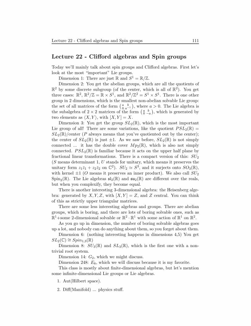
Lecture 22 - Clifford algebras and Spin groups 111
Lecture 22 - Clifford algebras and Spin groups
Today we’ll mainly talk about spin groups and Clifford algebras. First let’slook at the most “important” Lie groups.
Dimension 1: There are just R and S1 = R/Z.Dimension 2: You get the abelian groups, which are all the quotients of
R2 by some discrete subgroup (of the center, which is all of R2). You getthree cases: R2, R2/Z = R× S1, and R2/Z2 = S1 × S1. There is one othergroup in 2 dimensions, which is the smallest non-abelian solvable Lie group:the set of all matrices of the form
(a b0 a−1
), where a > 0. The Lie algebra is
the subalgebra of 2 × 2 matrices of the form(a b0 −a
), which is generated by
two elements as 〈X,Y 〉, with [X,Y ] = X.Dimension 3: You get the group SL2(R), which is the most important
Lie group of all! There are some variations, like the quotient PSL2(R) =SL2(R)/center (P always means that you’ve quotiented out by the center);the center of SL2(R) is just ±1. As we saw before, SL2(R) is not simplyconnected ... it has the double cover Mp2(R), which is also not simplyconnected. PSL2(R) is familiar because it acts on the upper half plane byfractional linear transformations. There is a compact version of this: SU2
(S means determinant 1, U stands for unitary, which means it preserves theunitary form z1z1 + z2z2 on C2). SU2 ≃ S3, and it surjects onto SO3(R),with kernel ±1 (O means it preserves an inner product). We also call SU2
Spin3(R). The Lie algebras sl2(R) and su2(R) are different over the reals,but when you complexify, they become equal.
There is another interesting 3-dimensional algebra: the Heisenberg alge-bra: generated by X,Y,Z, with [X,Y ] = Z, and Z central. You can thinkof this as strictly upper triangular matrices.
There are some less interesting algebras and groups. There are abeliangroups, which is boring, and there are lots of boring solvable ones, such asR1+some 2-dimensional solvable or R2 · R1 with some action of R1 on R2.
As you go up in dimension, the number of boring solvable algebras goesup a lot, and nobody can do anything about them, so you forget about them.
Dimension 6: (nothing interesting happens in dimensions 4,5) You getSL2(C) ∼= Spin1,3(R)
Dimension 8: SU3(R) and SL3(R), which is the first one with a non-trivial root system.
Dimension 14: G2, which we might discuss.Dimension 248: E8, which we will discuss because it is my favorite.This class is mostly about finite-dimensional algebras, but let’s mention
some infinite-dimensional Lie groups or Lie algebras.
1. Aut(Hilbert space).
2. Diff(Manifold) ... physics stuff.
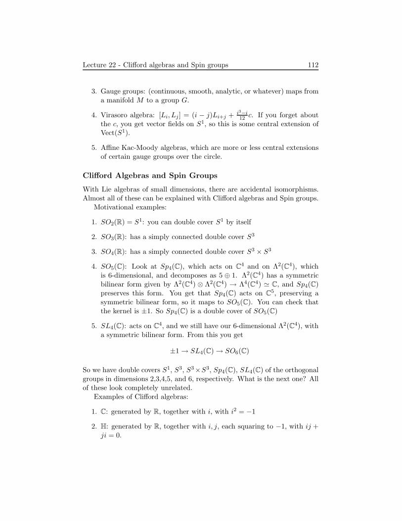
Lecture 22 - Clifford algebras and Spin groups 112
3. Gauge groups: (continuous, smooth, analytic, or whatever) maps froma manifold M to a group G.
4. Virasoro algebra: [Li, Lj ] = (i − j)Li+j + i3−i12 c. If you forget about
the c, you get vector fields on S1, so this is some central extension ofVect(S1).
5. Affine Kac-Moody algebras, which are more or less central extensionsof certain gauge groups over the circle.
Clifford Algebras and Spin Groups
With Lie algebras of small dimensions, there are accidental isomorphisms.Almost all of these can be explained with Clifford algebras and Spin groups.
Motivational examples:
1. SO2(R) = S1: you can double cover S1 by itself
2. SO3(R): has a simply connected double cover S3
3. SO4(R): has a simply connected double cover S3 × S3
4. SO5(C): Look at Sp4(C), which acts on C4 and on Λ2(C4), whichis 6-dimensional, and decomposes as 5 ⊕ 1. Λ2(C4) has a symmetricbilinear form given by Λ2(C4) ⊗ Λ2(C4) → Λ4(C4) ≃ C, and Sp4(C)preserves this form. You get that Sp4(C) acts on C5, preserving asymmetric bilinear form, so it maps to SO5(C). You can check thatthe kernel is ±1. So Sp4(C) is a double cover of SO5(C)
5. SL4(C): acts on C4, and we still have our 6-dimensional Λ2(C4), witha symmetric bilinear form. From this you get
±1 → SL4(C) → SO6(C)
So we have double covers S1, S3, S3×S3, Sp4(C), SL4(C) of the orthogonalgroups in dimensions 2,3,4,5, and 6, respectively. What is the next one? Allof these look completely unrelated.
Examples of Clifford algebras:
1. C: generated by R, together with i, with i2 = −1
2. H: generated by R, together with i, j, each squaring to −1, with ij +ji = 0.

Lecture 22 - Clifford algebras and Spin groups 113
3. Dirac wanted a square root for the operator ∂2
∂x2 + ∂2
∂y2+ ∂2
∂z2− ∂2
∂t2(the
wave operator in 4 dimensions). What he tried doing was supposingthat the square root is of the form A = γ1
∂∂x + γ2
∂∂y + γ3
∂∂z + γ4
∂∂t .
Then set A2 = ∇ and compare coefficients, and you find that γ21 = 1,
γ22 = 1, γ2
3 = 1, γ24 = −1, and γiγj + γjγi = 0 for i 6= j.
Dirac solved this by taking the γi to be 4 × 4 complex matrices. Theoperator A acts on vector-valued functions on space-time.
Definition 22.1. A general Clifford algebra over R should be generated byelements γ1, . . . , γn such that γ2
i is some given real, and γiγj + γjγi = 0 fori 6= j.
Definition 22.2 (better (invariant) definition). Suppose we have somevector space V over some field K (usually R), with some quadratic formN : V → K. Then the Clifford algebra over K is generated by the vectorspace V , with relations v2 = N(v).
Note that N(λv) = λ2N(v), and the expression (a, b) := N(a + b) −N(a)−N(b) is bilinear, so if the characteristic of K is not 2, we have N(a) =(a,a)
2 . Thus, you can work with the bilinear form instead of the quadraticform. We’ll use quadratic forms so that everything works in characteristic2.
Example 22.3. Take V = R2 with basis i, j, with N(xi+ yj) = −x2 − y2.Then the relations are (xi + yj)2 = −x2 − y2, which gives you exactly therelations for the quaternions.
Warning 22.4. A few authors (mainly in index theory) use the relationsv2 = −N(v). Some people add a factor of 2, which usually doesn’t
matter, but is wrong in characteristic 2.
Let’s work out a few more small examples:Cm,n(R) is the Clifford algebra over R of the quadratic form x2
1 + · · · +x2m − x2
m+1 − · · · − x2m+n (m pluses and n minuses).
Problem: Find the structure of all the Cm,n(R).We know that C0,0(R) is R
C1,0(R) is R[ε]/(ε2 − 1) = R⊕ RC0,1(R) is R[i]/(i2 + 1) = CC2,0(R) is R[α, β]/(α2 − 1, β2 − 1, αβ + βα), which we can model by α =(
1 00 −1
)and β =
(0 11 0
).
We have a homomorphism C2,0(R) → M2(R), which is onto (becausethe two matrices generate M2(R)); the dimension of the later is 4, and thedimension of C2,0(R) is at most 4 because it is spanned by 1, α, β, αβ. Sothis map is actually an isomorphism. Thus C2,0(R) ≃M2(R). Note that the
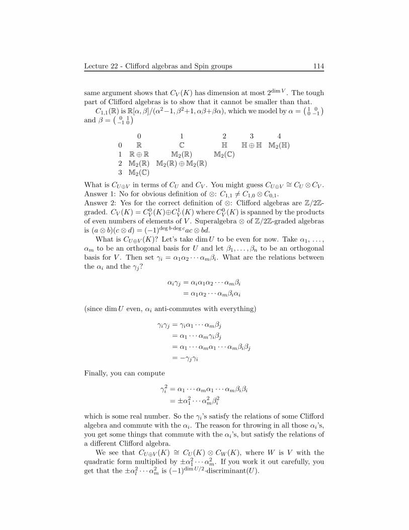
Lecture 22 - Clifford algebras and Spin groups 114
same argument shows that CV (K) has dimension at most 2dimV . The toughpart of Clifford algebras is to show that it cannot be smaller than that.
C1,1(R) is R[α, β]/(α2−1, β2+1, αβ+βα), which we model by α =(
1 00 −1
)
and β =(
0 1−1 0
)
0 1 2 3 40 R C H H⊕H M2(H)1 R⊕ R M2(R) M2(C)2 M2(R) M2(R) ⊕M2(R)3 M2(C)
What is CU⊕V in terms of CU and CV . You might guess CU⊕V ∼= CU ⊗CV .Answer 1: No for obvious definition of ⊗: C1,1 6= C1,0 ⊗ C0,1.Answer 2: Yes for the correct definition of ⊗: Clifford algebras are Z/2Z-graded. CV (K) = C0
V (K)⊕C1V (K) where C0
V (K) is spanned by the productsof even numbers of elements of V . Superalgebra ⊗ of Z/2Z-graded algebrasis (a⊗ b)(c ⊗ d) = (−1)deg b·deg cac⊗ bd.
What is CU⊕V (K)? Let’s take dimU to be even for now. Take α1, . . . ,αm to be an orthogonal basis for U and let β1, . . . , βn to be an orthogonalbasis for V . Then set γi = α1α2 · · ·αmβi. What are the relations betweenthe αi and the γj?
αiγj = αiα1α2 · · ·αmβi= α1α2 · · ·αmβiαi
(since dimU even, αi anti-commutes with everything)
γiγj = γiα1 · · ·αmβj= α1 · · ·αmγiβj= α1 · · ·αmα1 · · ·αmβiβj= −γjγi
Finally, you can compute
γ2i = α1 · · ·αmα1 · · ·αmβiβi
= ±α21 · · ·α2
mβ2i
which is some real number. So the γi’s satisfy the relations of some Cliffordalgebra and commute with the αi. The reason for throwing in all those αi’s,you get some things that commute with the αi’s, but satisfy the relations ofa different Clifford algebra.
We see that CU⊕V (K) ∼= CU (K) ⊗ CW (K), where W is V with thequadratic form multiplied by ±α2
1 · · ·α2m. If you work it out carefully, you
get that the ±α2l · · ·α2
m is (−1)dimU/2·discriminant(U).

Lecture 22 - Clifford algebras and Spin groups 115
Take dimU = 2 and see what we get. We find that Cm+2,n(R) ∼= M2(R)⊗Cn,m(R), where the indices have reversed because we have a factor of −1,so we must change the sign of the form, which means that we change thesubscripts. Similarly, we find that Cm+1,n+1(R) ∼= M2(R)⊗Cm,n(R), wherethe indices are in the right order. Finally, we have that Cm,n+2(R) ∼= H ⊗Cn,m(R). Using these formulas, we can reduce any Clifford algebra to tensorproducts of things like R, C, H, and M2(R).
Recall the rules for taking tensor products of matrix algebras:
1. R⊗X ∼= X
2. C ⊗ H ∼= M2(C) because all 2-dimensional quadratic forms look thesame over C
3. C⊗R C ∼= C⊕ C
4. H⊗C H ∼= M4(R), which you can see by thinking of the H’s by actingby left and right multiplication on R4.
5. Mm(Mn(X)) ∼= Mmn(X)
6. Mm(A) ⊗Mn(B) ∼= Mmn(A⊗B)
Now we can work out every possible real Clifford algebra: see the table1.You don’t need to fill in the middle because you just take Mn to M2n.
Then you find that C8+m,n∼= Cm,n⊗M16(R). You also get a mod 8 period-
icity going down.
1The table will look all wrong in the dvi; look at the pdf or ps instead.
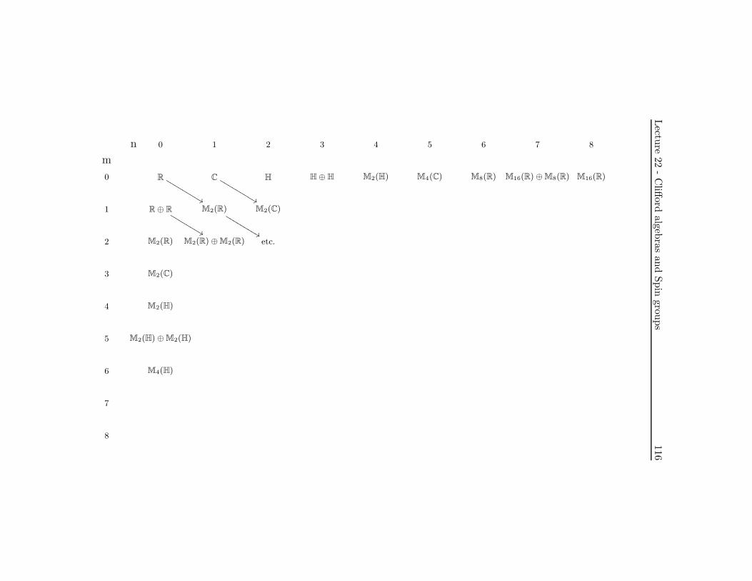
Lectu
re22
-C
lifford
algebras
and
Spin
groups
116
m
n 0 1 2 3 4 5 6 7 8
0 R
%%LLLLLLLLL C
%%LLLLLLLLL H H⊕H M2(H) M4(C) M8(R) M16(R) ⊕M8(R) M16(R)
1 R⊕ R
%%LLLLLLLL M2(R)
%%LLLLLLLLLM2(C)
2 M2(R) M2(R) ⊕M2(R) etc.
3 M2(C)
4 M2(H)
5 M2(H) ⊕M2(H)
6 M4(H)
7
8
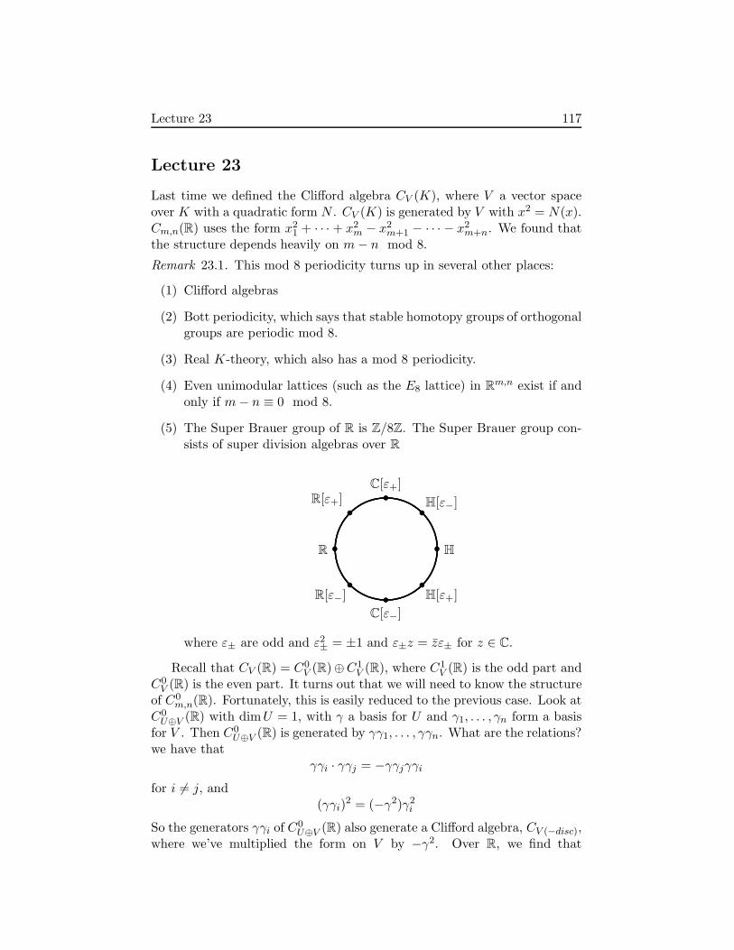
Lecture 23 117
Lecture 23
Last time we defined the Clifford algebra CV (K), where V a vector spaceover K with a quadratic form N . CV (K) is generated by V with x2 = N(x).Cm,n(R) uses the form x2
1 + · · · + x2m − x2
m+1 − · · · − x2m+n. We found that
the structure depends heavily on m− n mod 8.
Remark 23.1. This mod 8 periodicity turns up in several other places:
(1) Clifford algebras
(2) Bott periodicity, which says that stable homotopy groups of orthogonalgroups are periodic mod 8.
(3) Real K-theory, which also has a mod 8 periodicity.
(4) Even unimodular lattices (such as the E8 lattice) in Rm,n exist if andonly if m− n ≡ 0 mod 8.
(5) The Super Brauer group of R is Z/8Z. The Super Brauer group con-sists of super division algebras over R
R •
R[ε+]•
C[ε+]• H[ε−]•
H•
H[ε+]•
C[ε−]•R[ε−]
•
where ε± are odd and ε2± = ±1 and ε±z = zε± for z ∈ C.
Recall that CV (R) = C0V (R)⊕C1
V (R), where C1V (R) is the odd part and
C0V (R) is the even part. It turns out that we will need to know the structure
of C0m,n(R). Fortunately, this is easily reduced to the previous case. Look at
C0U⊕V (R) with dimU = 1, with γ a basis for U and γ1, . . . , γn form a basis
for V . Then C0U⊕V (R) is generated by γγ1, . . . , γγn. What are the relations?
we have thatγγi · γγj = −γγjγγi
for i 6= j, and(γγi)
2 = (−γ2)γ2i
So the generators γγi of C0U⊕V (R) also generate a Clifford algebra, CV (−disc),
where we’ve multiplied the form on V by −γ2. Over R, we find that

Lecture 23 118
C0m+1,n(R) ∼= Cn,m(R) and C1
m,n+1(R) ∼= Cm,n(R). So we’ve worked outall the real algebras and all the even and odd parts of them.
Remark 23.2. For Complex Clifford algebras, it is similar, but easier. Youfind that C2m(C) ∼= M2m(C) and C2m+1(C) ∼= M2m(C) ⊕M2m(C). Noticethat we have mod 2 periodicity now. Notice also that Bott periodicity forthe unitary group is mod 2. You could figure these out by tensoring the realalgebras with C if you wanted.
Clifford Groups
Usually the Clifford groups are denoted ΓV (K). We will show that ΓV (K)is a subgroup of CV (K)× and we’ll find an exact sequence
1 → K× central−−−−→ ΓV (K) → OV (K) → 1
Definition 23.3. ΓV (K) = homogeneous (either degree 1 or degree 0, notreally needed) invertible elements x of CV (K) such that xV α(x)−1 ⊆ V (recall that V ⊆ CV (K)), where α is the automorphism of CV (K) inducedby −1 on V .
Many books leave out the α, which is a mistake (though not a seriousone). Why do we use xV α(x)−1 instead of xV x−1, which is also possible?Reasons:
(1) It is the correct “superalgebra” sign. The superalgebra conventionsays that whenever you exchange two elements of odd degree, you putin a −1, and you think of V and x as odd.
(2) Putting α in makes the theory much cleaner in ODD dimensions. Forexample, we will get a map CV (K) → OV (K) which is onto if we useα, but not if we do not. (You get SOV (K) without the α, which isn’ttoo bad, but is still annoying.)
Lemma 23.4. 1 (V non-degenerate) The elements of ΓV (K) acting triviallyon V are the elements of K× ⊆ ΓV (K) ⊆ CV (K).
Proof. Suppose a0 + a1 ∈ Γ0V (K) + Γ1
V (K) acts trivially on V . Then (a0 +a1)v = v(a0−a1) (the minus sign comes because we’re using α), so a0v = va0
and a1v = −va1. Choose an orthogonal basis γ1, . . . , γn for V .2 Write a0 asa linear combination of monomials in this basis, so that
a0 = m+ γ1n
1I promised no Lemmas or Theorems, but I was lying to you.2All these results are true in characteristic 2, but you have to work harder ... you can’t
go around choosing orthogonal bases.

Lecture 23 119
where m ∈ C0V (K) and n ∈ C1
V (K) and neither m nor n contain a factor ofγ1. Apply the relations
a0v = va0 and a1v = −va1
with v = γ1 and use orthogonality to conclude that a0 contains no monomialwith a factor γ1. Repeat with v equal to the other basis elements. Similarly,write a1 as a linear combination of monomials in the basis, and apply therelations to v varying among the basis elements.
Exercise 23.1. Check that you must have a0 ∈ K and a1 = 0. (If youdon’t use α, a1 could be γ1 · · · γn when n is odd.)
So a0 + a1 = a0 ∈ K ∩ ΓV (K) = K∗.
Now we define the anti-automorphism T on CV (K) to be 1 on V , and ex-tend to CV (K) (anti means that (ab)T = bTaT ). Do not confuse a 7→α(a) (automorphism), a 7→ aT (anti-automorphism), and a 7→ α(aT ) (anti-automorphism).
Now we define the spinor norm N by N(a) = aaT , Nα(a) = aα(a)T fora ∈ CV (K). Main properties: (1)N is a homomorphism ΓV (K) → CV (K)with image in K× (N is a mess on the rest of CV (K)) and (2) the imageof ΓV (K) in AutV lies in OV (K). Notice that on V , N coincides withthe quadratic form N (many authors seem not to have noticed this, anduse different letters ... sometimes they use a stupid sign convention whichmakes them different).
Proof. We show that if a ∈ ΓV (K), then Nα(a) acts trivially on V . Calcu-late
α(Nα(a))v(Nα(a))−1 = α(a)aT vα(aT )−1a−1
= α(a)α(a−1)vaa−1 (apply T ; use T |V = 1)
= v
So by the previous lemma, Nα(a) ∈ K×.
This implies that Nα is a homomorphism on ΓV (K) because
Nα(a)Nα(b) = aα(a)TNα(b)
= aNα(b)α(a)T (Nα(b) is central)
= abα(b)Tα(a)T
= (ab)α(ab)T = Nα(ab)
After all this work with Nα, what we’re really interested is N . N = Nα
on Γ0V (K) and N = −Nα on Γ1
V (K). Since ΓV (K) = Γ0V (K)∪Γ1
V (K), which

Lecture 23 120
shows that N is also a homomorphism. Observe that the Clifford action onV preserves N on V because N is a homomorphism, but N |V is just thequadratic form on V . So we get a homomorphism from CV (K) → OV (K).What is its kernel, and is it surjective? The kernel is easy to figure out,because we did it a few minutes ago. The kernel is the elements of ΓV (K)acting trivially on V , which is just the elements of K×. Is it onto? To seethis, we should write some explicit elements. Say r ∈ V and N(r) 6= 0.Then r ∈ ΓV (K) (we’ll see this in a second). What is its action on V ?
rvα(r)−1 = −rv r
N(r)
= −r if v=r
= v if (v, r) = 0
So it acts by reflection through the hyperplane r⊥. This is another goodreason for putting the α ... you would get something more annoying other-wise. You might think that we’ll conclude that the map is surjective becauseOV (K) is generated by reflections. That’s wrong! Orthogonal groups neednot be generated by reflections.
Here is a counterexample. Take the field F2 and V = F42 = H⊕H, where
H is the quadratic form x2 + y2 + xy (each H has three elements of norm1). Then the reflections generate the group S3 × S3 of order 36 ... there isno way to flip the two H’s by reflections.
Exercise 23.2. check this
But the orthogonal group has order 72. It turns out that this is theONLY counterexample. Any other field, or any other non-degenerate formon any other space works just fine.
In fact, the map CV (K) → OV (K) is always onto even in the exam-ple above. For groups over R (which is what we are interested in in thiscourse), this follows easily from the fact that OV (R) is indeed generated byreflections.
Summarizing: We have the exact sequence
1 → K× → ΓV (K) → OV (K) → 1
where K× lands in the center of ΓV (K).
1 // K× //
‖
ΓV (K)
N
// OV (K) //
N
1
1 // K× x 7→x2// K× // K×/(K×)2 // 1
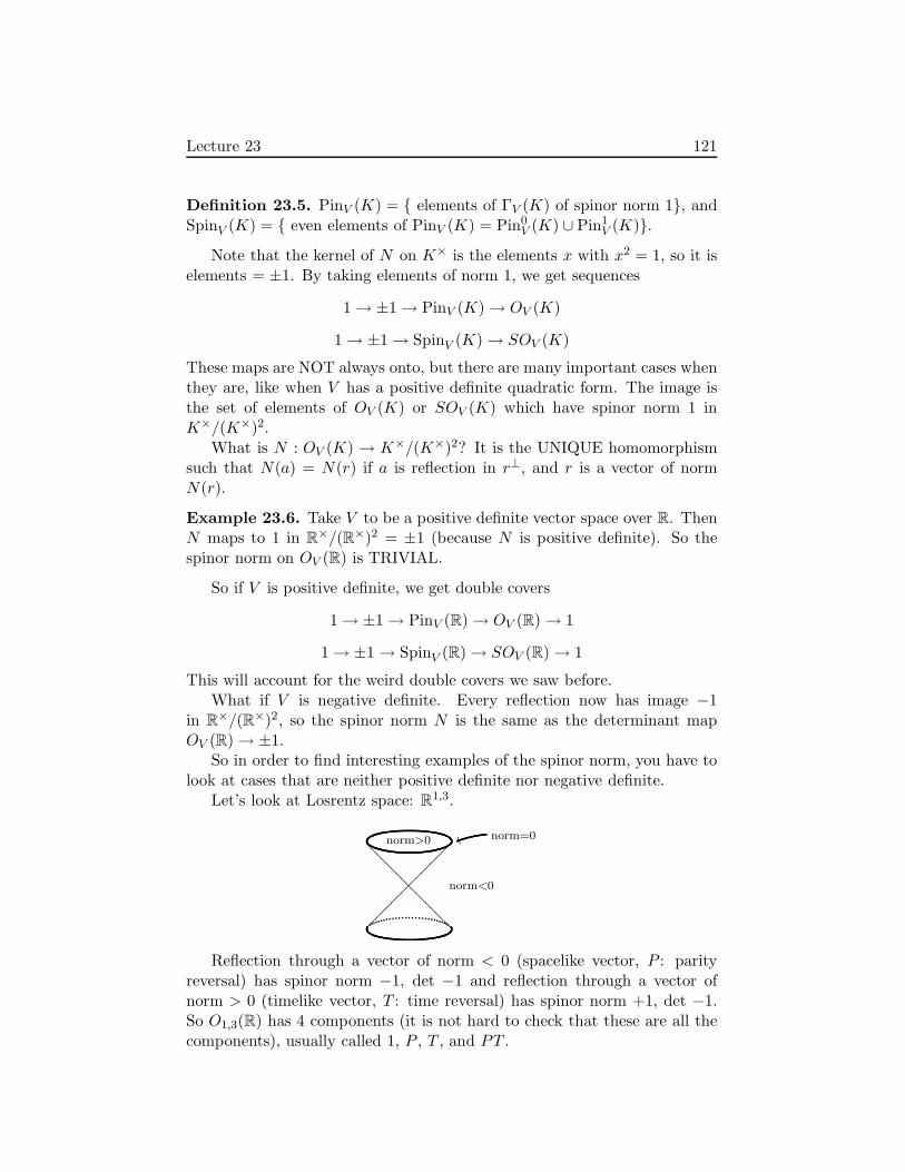
Lecture 23 121
Definition 23.5. PinV (K) = elements of ΓV (K) of spinor norm 1, andSpinV (K) = even elements of PinV (K) = Pin0
V (K) ∪ Pin1V (K).
Note that the kernel of N on K× is the elements x with x2 = 1, so it iselements = ±1. By taking elements of norm 1, we get sequences
1 → ±1 → PinV (K) → OV (K)
1 → ±1 → SpinV (K) → SOV (K)
These maps are NOT always onto, but there are many important cases whenthey are, like when V has a positive definite quadratic form. The image isthe set of elements of OV (K) or SOV (K) which have spinor norm 1 inK×/(K×)2.
What is N : OV (K) → K×/(K×)2? It is the UNIQUE homomorphismsuch that N(a) = N(r) if a is reflection in r⊥, and r is a vector of normN(r).
Example 23.6. Take V to be a positive definite vector space over R. ThenN maps to 1 in R×/(R×)2 = ±1 (because N is positive definite). So thespinor norm on OV (R) is TRIVIAL.
So if V is positive definite, we get double covers
1 → ±1 → PinV (R) → OV (R) → 1
1 → ±1 → SpinV (R) → SOV (R) → 1
This will account for the weird double covers we saw before.What if V is negative definite. Every reflection now has image −1
in R×/(R×)2, so the spinor norm N is the same as the determinant mapOV (R) → ±1.
So in order to find interesting examples of the spinor norm, you have tolook at cases that are neither positive definite nor negative definite.
Let’s look at Losrentz space: R1,3.
?????????????????
norm>0
norm<0
norm=0uu
Reflection through a vector of norm < 0 (spacelike vector, P : parityreversal) has spinor norm −1, det −1 and reflection through a vector ofnorm > 0 (timelike vector, T : time reversal) has spinor norm +1, det −1.So O1,3(R) has 4 components (it is not hard to check that these are all thecomponents), usually called 1, P , T , and PT .

Lecture 23 122
Remark 23.7. For those who know Galois cohomology. We get an exactsequence of algebraic groups
1 → GL1 → ΓV → OV → 1
(algebraic group means you don’t put a field). You do not necessarily getan exact sequence when you put in a field.
If1 → A→ B → C → 1
is exact,1 → A(K) → B(K) → C(K)
is exact. What you really get is
1 → H0(Gal(K/K), A) → H0(Gal(K/K), B) → H0(Gal(K/K), C) →→ H1(Gal(K/K), A) → · · ·
It turns out thatH1(Gal(K/K), GL1) = 1. However, H1(Gal(K/K),±1) =K×/(K×)2.
So from1 → GL1 → ΓV → OV → 1
you get
1 → K× → ΓV (K) → OV (K) → 1 = H1(Gal(K/K), GL1)
However, taking1 → µ2 → SpinV → SOV → 1
you get
1 → ±1 → SpinV (K) → SOV (K)N−→ K×/(K×)2 = H1(K/K, µ2)
so the non-surjectivity of N is some kind of higher Galois cohomology.
Warning 23.8. SpinV → SOV is onto as a map of ALGEBRAICGROUPS, but SpinV (K) → SOV (K) need NOT be onto.
Example 23.9. Take O3(R) ∼= SO3(R) × ±1 as 3 is odd (in generalO2n+1(R) ∼= SO2n+1(R) × ±1). So we have a sequence
1 → ±1 → Spin3(R) → SO3(R) → 1.
Notice that Spin3(R) ⊆ C03 (R) ∼= H, so Spin3(R) ⊆ H×, and in fact we saw
that it is S3.

Lecture 24 123
Lecture 24
Last time we constructed the sequences
1 → K× → ΓV (K) → OV (K) → 1
1 → ±1 → PinV (K) → OV (K)N−→ K×/(K×)2
1 → ±1 → SpinV (K) → SOV (K)N−→ K×/(K×)2
Spin representations of Spin and Pin groups
Notice that PinV (K) ⊆ CV (K)×, so any module over CV (K) gives a repre-sentation of PinV (K). We already figured out that CV (K) are direct sumsof matrix algebras over R,C, and H.
What are the representations (modules) of complex Clifford algebras?Recall that C2n(C) ∼= M2n(C), which has a representations of dimension2n, which is called the spin representation of PinV (K) and C2n+1(C) ∼=M2n(C) ×M2n(C), which has 2 representations, called the spin representa-tions of Pin2n+1(K).
What happens if we restrict these to SpinV (C) ⊆ PinV (C)? To do that,we have to recall that C0
2n(C) ∼= M2n−1(C) × M2n−1(C) and C02n+1(C) ∼=
M2n(C). So in EVEN dimensions Pin2n(C) has 1 spin representation ofdimension 2n splitting into 2 HALF SPIN representations of dimension 2n−1
and in ODD dimensions, Pin2n+1(C) has 2 spin representations of dimension2n which become the same on restriction to SpinV (C).
Now we’ll give a second description of spin representations. We’ll justdo the even-dimensional case (odd is similar). Say dimV = 2n, and saywe’re over C. Choose an orthonormal basis γ1, . . . , γ2n for V , so that γ2
i = 1and γiγj = −γjγi. Now look at the group G generated by γ1, . . . , γ2n, whichis finite, with order 21+2n (you can write all its elements explicitly). Youcan see that representations of CV (C) correspond to representations of G,with −1 acting as −1 (as opposed to acting as 1). So another way to lookat representations of the Clifford algebra, you can look at representations ofG.
Let’s look at the structure of G:
(1) The center is ±1. This uses the fact that we are in even dimensions,lest γ1 · · · γ2n also be central.
(2) The conjugacy classes: 2 of size 1 (1 and −1), 22n − 1 of size 2(±γi1 · · · γin), so we have a total of 22n + 1 conjugacy classes, so weshould have that many representations. G/center is abelian, isomor-phic to (Z/2Z)2n, which gives us 22n representations of dimension 1,

Lecture 24 124
so there is only one more left to find! We can figure out its dimensionby recalling that the sum of the squares of the dimensions of irre-ducible representations gives us the order of G, which is 22n+1. So22n × 11 + 1 × d2 = 22n+1, where d is the dimension of the mysteryrepresentation. Thus, d = ±2n, so d = 2n. Thus, G, and thereforeCV (C), has an irreducible representation of dimension 2n (as we foundearlier in another way).
Example 24.1. Consider O2,1(R). As before, O2,1(R) ∼= SO2,1(R) × (±1),and SO2,1(R) is not connected: it has two components, separated by thespinor norm N . We have maps
1 → ±1 → Spin2,1(R) → SO2,1(R)N−→ ±1.
Spin2,1(R) ⊆ C∗2,1(R) ∼= M2(R), so Spin2,1(R) has one 2-dimensional spin
representation. So there is a map Spin2,1(R) → SL2(R); by counting dimen-sions and such, you can show it is an isomorphism. So Spin2,1(R) ∼= SL2(R).
Now let’s look at some 4-dimensional orthogonal groups
Example 24.2. Look at SO4(R), which is compact. It has a complexspin representation of dimension 24/2 = 4, which splits into two half spinrepresentations of dimension 2. We have the sequence
1 → ±1 → Spin4(R) → SO4(R) → 1 (N = 1)
Spin4(R) is also compact, so the image in any complex representation iscontained in some unitary group. So we get two maps Spin4(R) → SU(2)×SU(2), and both sides have dimension 6 and centers of order 4. Thus, wefind that Spin4(R) ∼= SU(2)×SU(2) ∼= S3×S3, which give you the two halfspin representations.
So now we’ve done the positive definite case.
Example 24.3. Look at SO3,1(R). Notice that O3,1(R) has four compo-nents distinguished by the maps det, N → ±1. So we get
1 → ±1 → Spin3,1(R) → SO3,1(R)N−→ ±1 → 1
We expect 2 half spin representations, which give us two homomorphismsSpin3,1(R) → SL2(C). This time, each of these homomorphisms is an iso-morphism (I can’t think of why right now). The SL2(C)s are double coversof simple groups. Here, we don’t get the splitting into a product as in thepositive definite case. This isomorphism is heavily used in quantum fieldtheory because Spin3,1(R) is a double cover of the connected component of

Lecture 24 125
the Lorentz group (and SL2(C) is easy to work with). Note also that thecenter of Spin3,1(R) has order 2, not 4, as for Spin4,0(R). Also note that
the group PSL2(C) acts on the compactified C ∪ ∞ by(a bc d
)(τ) = aτ+b
cτ+d .Subgroups of this group are called KLEINIAN groups. On the other hand,the group SO3,1(R)+ (identity component) acts on H3 (three-dimensionalhyperbolic space). To see this, look at
????
??
???
norm=−1oo
norm=0uu
norm=−1uu
norm=1uu
One sheet of norm −1 hyperboloid is isomorphic to H3 under the inducedmetric. In fact, we’ll define hyperbolic space that way. If you’re a topolo-gist, you’re very interested in hyperbolic 3-manifolds, which are H3/(discretesubgroup of SO3,1(R)). If you use the fact that SO3,1(R) ∼= PSL2(R), thenyou see that these discrete subgroups are in fact Klienian groups.
There are lots of exceptional isomorphisms in small dimension, all ofwhich are very interesting, and almost all of them can be explained by spingroups.
Example 24.4. O2,2(R) has 4 components (given by det, N); C02,2(R) ∼=
M2(R) × M2(R), which induces an isomorphism Spin2,2(R) → SL2(R) ×SL2(R), which give you the two half spin representations. Both sides havedimension 6 with centers of order 4. So this time we get two non-compactgroups. Let’s look at the fundamental group of SL2(R), which is Z, so thefundamental group of Spin2,2(R) is Z ⊕ Z. As we recall, Spin4,0(R) andSpin3,1(R) were both simply connected. This shows that SPIN GROUPSNEED NOT BE SIMPLY CONNECTED. So we can take covers of it. Whatdo the corresponding covers (e.g. the universal cover) of Spin2,2(R) looklike? This is hard to describe because for FINITE dimensional complexrepresentations, you get finite dimensional representations of the lie algebraL, which correspond to the finite-dimensional representations of L⊗C, whichcorrespond to the finite-dimensional representations of L′ = Lie algebraof Spin4,0(R), which correspond to the finite-dimensional representationsof Spin4,0(R), which has no covers because it is simply connected. Thismeans that any finite-dimensional representation of a cover of Spin2,2(R)actually factors through Spin2,2(R). So there is no way you can talk about

Lecture 24 126
these things with finite matrices, and infinite-dimensional representationsare hard.
To summarize, the ALGEBRAIC GROUP Spin2,2 is simply connected(as an algebraic group) (think of an algebraic group as a functor from rings togroups), which means that it has no algebraic central extensions. However,the LIE GROUP Spin2,2(R) is NOT simply connected; it has fundamentalgroup Z ⊕ Z. This problem does not happen for COMPACT Lie groups(where every finite cover is algebraic).
We’ve done O4,0, O3,1, and O2,2, from which we can obviously get O1,3
and O0,4. Note that O4,0(R) ∼= O0,4(R), SO4,0(R) ∼= SO0,4(R), Spin4,0(R) ∼=Spin0,4(R). However, Pin4,0(R) 6∼= Pin0,4(R). These two are hard to distin-guish. We have
Pin4,0(R)
Pin0,4(R)
O4,0(R) = O0,4(R)
Take a reflection (of order 2) in O4,0(R), and lift it to the Pin groups. Whatis the order of the lift? The reflection vector v, with v2 = ±1 lifts to theelement v ∈ ΓV (R) ⊆ C∗
V (R). Notice that v2 = 1 in the case of R4,0 andv2 = −1 in the case of R0,4, so in Pin4,0(R), the reflection lifts to somethingof order 2, but in Pin0,4(R), you get an element of order 4!. So these twogroups are different.
Two groups are isoclinic if they are confusingly similar. A similar phe-nomenon is common for groups of the form 2 · G · 2, which means it has acenter of order 2, then some group G, and the abelianization has order 2.Watch out.
Exercise 24.1. Spin3,3(R) ∼= SL4(R).
Triality
This is a special property of 8-dimensional orthogonal groups. Recall thatO8(C) has the Dynkin diagram D4, which has a symmetry of order three:
11
111
00
ZZ
But O8(C) and SO8(C) do NOT have corresponding symmetries of or-der three. The thing that does have the symmetry of order three is thespin group! The group Spin8(R) DOES have “extra” order three symme-try. You can see it as follows. Look at the half spin representations of

Lecture 24 127
Spin8(R). Since this is a spin group in even dimension, there are two.C8,0(R) ∼= M28/2−1(R) × M28/2−1(R) ∼= M8(R) ×M8(R). So Spin8(R) hastwo 8-dimensional real half spin representations. But the spin group is com-pact, so it preserves some quadratic form, so you get 2 homomorphismsSpin8(R) → SO8(R). So Spin8(R) has THREE 8-dimensional representa-tions: the half spins, and the one from the map to SO8(R). These mapsSpin8(R) → SO8(R) lift to Triality automorphisms Spin8(R) → Spin8(R).The center of Spin8(R) is (Z/2) + (Z/2) because the center of the Cliffordgroup is ±1,±γ1 · · · γ8. There are 3 non-trivial elements of the center, andquotienting by any of these gives you something isomorphic to SO8(R). Thisis special to 8 dimensions.
More about Orthogonal groups
Is OV (K) a simple group? NO, for the following reasons:
(1) There is a determinant map OV (K) → ±1, which is usually onto, soit can’t be simple.
(2) There is a spinor norm map OV (K) → K×/(K×)2
(3) −1 ∈ center of OV (K).
(4) SOV (K) tends to split if dimV = 4, abelian if dimV = 2, and trivialif dimV = 1.
It turns out that they are usually simple apart from these four reasons whythey’re not. Let’s mod out by the determinant, to get to SO, then look atSpinV (K), then quotient by the center, and assume that dimV ≥ 5. Thenthis is usually simple. The center tends to have order 1,2, or 4. If K is aFINITE field, then this gives many finite simple groups.
Note that SOV (K) is NOT a subgroup of OV (K), elements of determi-nant 1 in general, it is the image of Γ0
V (K) ⊆ ΓV (K) → OV (K), which is thecorrect definition. Let’s look at why this is right and the definition you knowis wrong. There is a homomorphism ΓV (K) → Z/2Z, which takes Γ0
V (K) to0 and Γ1
V (K) to 1 (called the DICKSON INVARIANT). It is easy to checkthat det(v) = (−1)dickson invariant(v). So if the characteristic of K is not 2,det = 1 is equivalent to dickson = 0, but in characteristic 2, determinant isthe wrong invariant (because determinant is always 1).
Special properties of O1,n(R) and O2,n(R). O1,n(R) acts on hyperbolicspace Hn, which is a component of norm −1 vectors in Rn,1. O2,n(R) acts onthe “Hermitian symmetric space” (Hermitian means it has a complex struc-ture, and symmetric means really nice). There are three ways to constructthis space:
Lecture 24 128
(1) It is the set of positive definite 2-dimensional subspaces of R2,n
(2) It is the norm 0 vectors ω of PC2,n with (ω, ω) = 0.
(3) It is the vectors x+ iy ∈ R1,n−1 with y ∈ C, where the cone C is theinterior of the norm 0 cone.
Exercise 24.2. Show that these are the same.
Next week, we’ll mess around with E8.

Lecture 25 - E8 129
Lecture 25 - E8
In this lecture we use a vector notation in which powers represent repetitions:so (18) = (1, 1, 1, 1, 1, 1, 1, 1) and (±1
22, 06) = (±1
2 ,±12 , 0, 0, 0, 0, 0, 0).
Recall that E8 has the Dynkin diagram
e1 − e2 e2 − e3
e3 − e4 e4 − e5
e5 − e6
(−12
5, 1
2
3) e6 − e7
e7 − e8
where each vertex is a root r with (r, r) = 2; (r, s) = 0 when r and s are notjoined, and (r, s) = −1 when r and s are joined. We choose an orthonormalbasis e1, . . . , e8, in which the roots are as given.
We want to figure out what the root lattice L of E8 is (this is thelattice generated by the roots). If you take ei − ei+1 ∪ (−15, 13) (allthe A7 vectors plus twice the strange vector), they generate the D8 lattice= (x1, . . . , x8)|xi ∈ Z,
∑xi even. So the E8 lattice consists of two cosets
of this lattice, where the other coset is (x1, . . . , x8)|xi ∈ Z+ 12 ,
∑xi odd.
Alternative version: If you reflect this lattice through the hyperplane e⊥1 ,then you get the same thing except that
∑xi is always even. We will freely
use both characterizations, depending on which is more convenient for thecalculation at hand.
We should also work out the weight lattice, which is the vectors s suchthat (r, r)/2 divides (r, s) for all roots r. Notice that the weight lattice ofE8 is contained in the weight lattice of D8, which is the union of four cosetsof D8: D8, D8 + (1, 07), D8 + (1
2
8) and D8 + (−1
2 ,12
7). Which of these have
integral inner product with the vector (−12
5, 1
2
3)? They are the first and the
last, so the weight lattice of E8 is D8 ∪D8 + (−12 ,
127), which is equal to the
root lattice of E8.In other words, the E8 lattice L is UNIMODULAR (equal to its dual
L′), where the dual is the lattice of vectors having integral inner productwith all lattice vectors. This is also true of G2 and F4, but is not in generaltrue of Lie algebra lattices.
The E8 lattice is EVEN, which means that the inner product of anyvector with itself is always even.
Even unimodular lattices in Rn only exist if 8|n (this 8 is the same 8that shows up in the periodicity of Clifford groups). The E8 lattice is theonly example in dimension equal to 8 (up to isomorphism, of course). Thereare two in dimension 16 (one of which is L ⊕ L, the other is D16∪ somecoset). There are 24 in dimension 24, which are the Niemeier lattices. In 32dimensions, there are more than a billion!

Lecture 25 - E8 130
The Weyl group of E8 is generated by the reflections through s⊥ wheres ∈ L and (s, s) = 2 (these are called roots). First, let’s find all the roots:(x1, . . . , x8) such that
∑x2i = 2 with xi ∈ Z or Z + 1
2 and∑xi even. If
xi ∈ Z, obviously the only solutions are permutations of (±1,±1, 06), ofwhich there are
(82
)× 22 = 112 choices. In the Z + 1
2 case, you can choosethe first 7 places to be ±1
2 , and the last coordinate is forced, so there are 27
choices. Thus, you get 240 roots.Let’s find the orbits of the roots under the action of the Weyl group.
We don’t yet know what the Weyl group looks like, but we can find alarge subgroup that is easy to work with. Let’s use the Weyl group ofD8, which consists of the following: we can apply all permutations of thecoordinates, or we can change the sign of an even number of coordinates(e.g., reflection in (1,−1, 06) swaps the first two coordinates, and reflectionin (1, −1, 06) followed by reflection in (1, 1, 06) changes the sign of the firsttwo coordinates.)
Notice that under the Weyl group of D8, the roots form two orbits: theset which is all permutations of (±12, 06), and the set (±1
2
8). Do these
become the same orbit under the Weyl group of E8? Yes; to show this,we just need one element of the Weyl group of E8 taking some element ofthe first orbit to the second orbit. Take reflection in (1
2
8)⊥ and apply it to
(12, 06): you get (12
2,−1
2
6), which is in the second orbit. So there is just one
orbit of roots under the Weyl group.What do orbits of W (E8) on other vectors look like? We’re interested in
this because we might want to do representation theory. The character of arepresentation is a map from weights to integers, which is W (E8)-invariant.Let’s look at vectors of norm 4 for example. So
∑x2i = 4,
∑xi even, and
xi ∈ Z or xi ∈ Z+ 12 . There are 8×2 possibilities which are permutations of
(±2, 07). There are(84
)× 24 permutations of (±14, 04), and there are 8× 27
permutations of (±32 ,±1
2
7). So there are a total of 240 × 9 of these vectors.
There are 3 orbits under W (D8), and as before, they are all one orbit under
the action of W (E8). Just reflect (2, 07) and (13,−1, 04) through (12
8).
Exercise 25.1. Show that the number of norm 6 vectors is 240×28, andthey form one orbit
(If you’ve seen a course on modular forms, you’ll know that the numberof vectors of norm 2n is given by 240 ×∑d|n d
3. If you let call these cn,then
∑cnq
n is a modular form of level 1 (E8 even, unimodular), weight 4(dimE8/2).)
For norm 8 there are two orbits, because you have vectors that are twicea norm 2 vector, and vectors that aren’t. As the norm gets bigger, you’llget a large number of orbits.

Lecture 25 - E8 131
What is the order of the Weyl group of E8? We’ll do this by 4 differentmethods, which illustrate the different techniques for this kind of thing:
(1) This is a good one as a mnemonic. The order of E8 is given by
|W (E8)| = 8! ×∏(
numbers on the
affine E8 diagram1
)
× Weight lattice of E8
Root lattice of E8
= 8!×(
1
2
3
4
5
6 3
4
2 )
× 1
= 214 × 35 × 52 × 7
We can do the same thing for any other Lie algebra, for example,
|W (F4)| = 4! × (1 2 3 4 // 2 ) × 1
= 27 × 32
(2) The order of a reflection group is equal to the products of degrees ofthe fundamental invariants. For E8, the fundamental invariants are ofdegrees 2,8,12,14,18,20,24,30 (primes +1).
(3) This one is actually an honest method (without quoting weird facts).The only fact we will use is the following: suppose G acts transitivelyon a set X with H = the group fixing some point; then |G| = |H| · |X|.This is a general purpose method for working out the orders of groups.First, we need a set acted on by the Weyl group of E8. Let’s take theroot vectors (vectors of norm 2). This set has 240 elements, and theWeyl group of E8 acts transitively on it. So |W (E8)| = 240×|subgroupfixing (1,−1, 06)|. But what is the order of this subgroup (call it G1)?Let’s find a set acted on by this group. It acts on the set of norm 2vectors, but the action is NOT transitive. What are the orbits? G1
fixes s = (1,−1, 06). For other roots r, G1 obviously fixes (r, s). Sohow many roots are there with a given inner product with s?
(s, r) number choices
2 1 s
1 56 (1, 0,±16), (0,−1,±16), (12 ,−1
2 ,126)
0 126−1 56−2 1 −s
1These are the numbers giving highest root.

Lecture 25 - E8 132
So there are at least 5 orbits under G1. In fact, each of these sets is asingle orbit under G1. How can we see this? Find a large subgroup ofG1. Take W (D6), which is all permutations of the last 6 coordinatesand all even sign changes of the last 6 coordinates. It is generated byreflections associated to the roots orthogonal to e1 and e2 (those thatstart with two 0s). The three cases with inner product 1 are threeorbits under W (D6). To see that there is a single orbit under G1, wejust need some reflections that mess up these orbits. If you take avector (1
2 ,12 ,±1
2
6) and reflect norm 2 vectors through it, you will get
exactly 5 orbits. So G1 acts transitively on these orbits.
We’ll use the orbit of vectors r with (r, s) = −1. Let G2 be the vectorsfixing s and r: s r We have that |G1| = |G2| · 56.Keep going ... it gets tedious, but here are the answers up to the laststep:
Our plan is to chose vectors acted on by Gi, fixed by Gi+1 which giveus the Dynkin diagram of E8. So the next step is to try to find vectors
t that give us the picture s r t , i.e, they have inner product−1 with r and 0 with s. The possibilities for t are (−1,−1, 0, 05) (oneof these), (0, 0, 1,±1, 04) and permutations of its last five coordinates
(10 of these), and (−12 ,−1
2 ,12 ,±1
2
5) (there are 16 of these), so we get 27
total. Then we could check that they form one orbit, which is boring.
Next find vectors which go next to t in our picture:s r t , i.e., whose inner product is −1 with t and zerowith r, s. The possibilities are permutations of the last four coords of(0, 0, 0, 1,±1, 03) (8 of these) and (−1
2 ,−12 ,−1
2 ,12 ,±1
24) (8 of these), so
there are 16 total. Again check transitivity.
Find a fifth vector; the possibilities are (04, 1,±1, 02) and perms of the
last three coords (6 of these), and (−12
4, 1
2 ,±12
3) (4 of these) for a total
of 10.
For the sixth vector, we can have (05, 1,±1, 0) or (05, 1, 0,±1) (4 pos-
sibilites) or (−12
5, 1
2 ,±12
2) (2 possibilities), so we get 6 total.
NEXT CASE IS TRICKY: finding the seventh one, the possibilitiesare (06, 1,±1) (2 of these) and ((−1
2)6, 12 ,
12 ) (just 1). The proof of tran-
sitivity fails at this point. The group we’re using by now doesn’t evenact transitively on the pair (you can’t get between them by chang-ing an even number of signs). What elements of W (E8) fix all of
these first 6 pointss r t ? We want to find
roots perpendicular to all of these vectors, and the only possibility is((1
2 )8). How does reflection in this root act on the three vectors above?
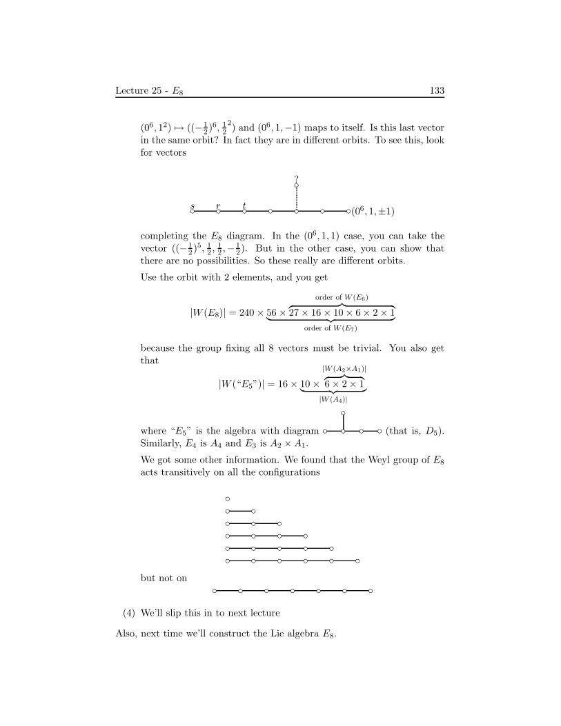
Lecture 25 - E8 133
(06, 12) 7→ ((−12 )6, 1
22) and (06, 1,−1) maps to itself. Is this last vector
in the same orbit? In fact they are in different orbits. To see this, lookfor vectors
s r t
?
(06, 1,±1)
completing the E8 diagram. In the (06, 1, 1) case, you can take thevector ((−1
2 )5, 12 ,
12 ,−1
2). But in the other case, you can show thatthere are no possibilities. So these really are different orbits.
Use the orbit with 2 elements, and you get
|W (E8)| = 240 × 56 ×order of W (E6)
︷ ︸︸ ︷
27 × 16 × 10 × 6 × 2 × 1︸ ︷︷ ︸
order of W (E7)
because the group fixing all 8 vectors must be trivial. You also getthat
|W (“E5”)| = 16 × 10 ×|W (A2×A1)|︷ ︸︸ ︷
6 × 2 × 1︸ ︷︷ ︸
|W (A4)|
where “E5” is the algebra with diagram
(that is, D5).Similarly, E4 is A4 and E3 is A2 ×A1.
We got some other information. We found that the Weyl group of E8
acts transitively on all the configurations
but not on
(4) We’ll slip this in to next lecture
Also, next time we’ll construct the Lie algebra E8.
Lecture 26 134
Lecture 26
Today we’ll finish looking at W (E8), then we’ll construct E8.Remember that we still have a fourth method of finding the order of
W (E8). Let L be the E8 lattice. Look at L/2L, which has 256 elements.Look at this as a set acted on by W (E8). There is an orbit of size 1 (repre-sented by 0). There is an orbit of size 240/2 = 120, which are the roots (aroot is congruent mod 2L to it’s negative). Left over are 135 elements. Let’slook at norm 4 vectors. Each norm 4 vector, r, satisfies r ≡ −r mod 2, andthere are 240 ·9 of them, which is a lot, so norm 4 vectors must be congruentto a bunch of stuff. Let’s look at r = (2, 0, 0, 0, 0, 0, 0, 0). Notice that it iscongruent to vectors of the form (0 · · · ± 2 . . . 0), of which there are 16. Itis easy to check that these are the only norm 4 vectors congruent to r mod2. So we can partition the norm 4 vectors into 240 · 9/16 = 135 subsets of16 elements. So L/2L has 1+120+135 elements, where 1 is the zero, 120 isrepresented by 2 elements of norm 2, and 135 is represented by 16 elementsof norm 4. A set of 16 elements of norm 4 which are all congruent is called aFRAME. It consists of elements ±e1, . . . ,±e8, where e2i = 4 and (ei, ej) = 1for i 6= j, so up to sign it is an orthogonal basis.
Then we have
|W (E8)| = (# frames) × |subgroup fixing a frame|
because we know that W (E8) acts transitively on frames. So we need toknow what the automorphisms of an orthogonal base are. A frame is 8 sub-sets of the form (r,−r), and isometries of a frame form the group (Z/2Z)8·S8,but these are not all in the Weyl group. In the Weyl group, we found a(Z/2Z)7 · S8, where the first part is the group of sign changes of an EVENnumber of coordinates. So the subgroup fixing a frame must be in betweenthese two groups, and since these groups differ by a factor of 2, it must beone of them. Observe that changing an odd number of signs doesn’t preservethe E8 lattice, so it must be the group (Z/2Z)7 · S8, which has order 27 · 8!.So the order of the Weyl group is
135 · 27 · 8! = |27 · S8| ×# norm 4 elements
2 × dimL
Remark 26.1. Similarly, if Λ is the Leech lattice, you actually get the orderof Conway’s group to be
|212 ·M24| ·# norm 8 elements
2 × dimΛ
where M24 is the Mathieu group (one of the sporadic simple groups). TheLeech lattice seems very much to be trying to be the root lattice of the
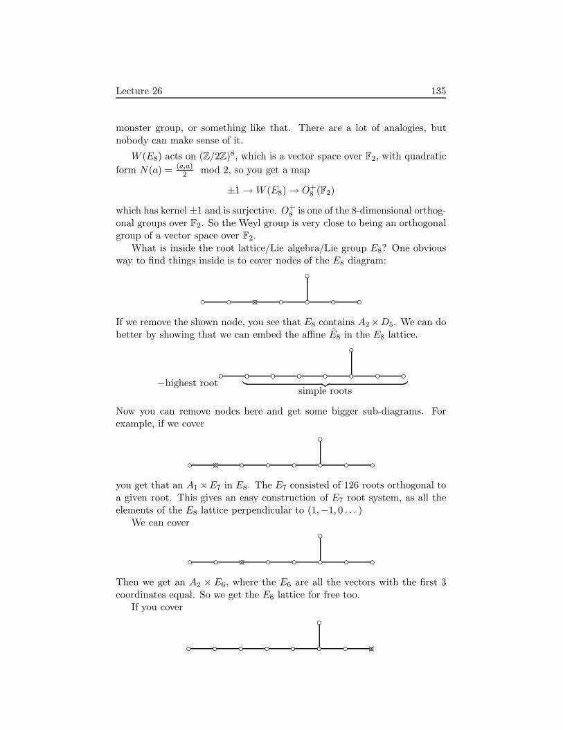
Lecture 26 135
monster group, or something like that. There are a lot of analogies, butnobody can make sense of it.
W (E8) acts on (Z/2Z)8, which is a vector space over F2, with quadratic
form N(a) = (a,a)2 mod 2, so you get a map
±1 → W (E8) → O+8 (F2)
which has kernel ±1 and is surjective. O+8 is one of the 8-dimensional orthog-
onal groups over F2. So the Weyl group is very close to being an orthogonalgroup of a vector space over F2.
What is inside the root lattice/Lie algebra/Lie group E8? One obviousway to find things inside is to cover nodes of the E8 diagram:
×
If we remove the shown node, you see that E8 contains A2 ×D5. We can dobetter by showing that we can embed the affine E8 in the E8 lattice.
−highest root
︸ ︷︷ ︸
simple roots
Now you can remove nodes here and get some bigger sub-diagrams. Forexample, if we cover
×
you get that an A1 ×E7 in E8. The E7 consisted of 126 roots orthogonal toa given root. This gives an easy construction of E7 root system, as all theelements of the E8 lattice perpendicular to (1,−1, 0 . . . )
We can cover
×
Then we get an A2 × E6, where the E6 are all the vectors with the first 3coordinates equal. So we get the E6 lattice for free too.
If you cover
×

Lecture 26 136
you see that there is a D8 in E8, which is all vectors of the E8 lattice withinteger coordinates. We sort of constructed the E8 lattice this way in thefirst place.
We can ask questions like: What is the E8 Lie algebra as a representationof D8? To answer this, we look at the weights of the E8 algebra, consideredas a module over D8, which are the 112 roots of the form (· · · ±1 · · · ±1 . . . )and the 128 roots of the form (±1/2, . . . ) and 1 vector 0, with multiplicity8. These give you the Lie algebra of D8. Recall that D8 is the Lie alge-bra of SO16. The double cover has a half spin representation of dimension216/2−1 = 128. So E8 decomposes as a representation of D8 as the adjointrepresentation (of dimension 120) plus a half spin representation of dimen-sion 128. This is often used to construct the Lie algebra E8. We’ll do abetter construction in a little while.
We’ve found that the Lie algebra of D8, which is the Lie algebra of SO16,is contained in the Lie algebra of E8. Which group is contained in the thecompact form of the E8? We found that there were groups
Spin16(R)
hhhhhhhhhhXXXXXXXXXXX
SO16(R)
VVVVVVVVV Spin16(R)/(Z/2Z) ∼= ?> =<89 :;Spin16(R)/(Z/2Z)
fffffffffff
PSO16(R)
corresponding to subgroups of the center (Z/2Z)2:
1
kkkkkkkkk
SSSSSSSSS
Z/2ZRRRRRR Z/2Z Z/2Z
llllll
(Z/2Z)2
We have a homomorphism Spin16(R) → E8(compact). What is the kernel?The kernel are elements which act trivially on the Lie algebra of E8, whichis equal to the Lie algebra D8 plus the half spin representation. On theLie algebra of D8, everything in the center is trivial, and on the half spinrepresentation, one of the elements of order 2 is trivial. So the subgroupthat you get is the circled one.
Exercise 26.1. Show SU(2) × E7(compact)/(−1,−1) is a subgroup ofE8 (compact). Similarly, show that SU(9)/(Z/3Z) is also. These are similarto the example above.
Construction of E8
Earlier in the course, we had some constructions:

Lecture 26 137
1. using the Serre relations, but you don’t really have an idea of what itlooks like
2. Take D8 plus a half spin representation
Today, we’ll try to find a natural map from root lattices to Lie algebras.The idea is as follows: Take a basis element eα (as a formal symbol) foreach root α; then take the Lie algebra to be the direct sum of 1-dimensionalspaces generated by each eα and L (L root lattice ∼= Cartan subalgebra) .Then we have to define the Lie bracket by setting [eα, eβ] = eα+β , but thenwe have a sign problem because [eα, eβ ] 6= −[eβ, eα]. Is there some way toresolve the sign problem? The answer is that there is no good way to solvethis problem (not true, but whatever). Suppose we had a nice functor fromroot lattices to Lie algebras. Then we would get that the automorphismgroup of the lattice has to be contained in the automorphism group of theLie algebra (which is contained in the Lie group), and the automorphismgroup of the Lattice contains the Weyl group of the lattice. But the Weylgroup is NOT usually a subgroup of the Lie group.
We can see this going wrong even in the case of sl2(R). Remember thatthe Weyl group is N(T )/T where T =
(a 00 a−1
)and N(T ) = T ∪
(0 b
−b−1 0
),
and this second part is stuff having order 4, so you cannot possibly writethis as a semi-direct product of T and the Weyl group.
So the Weyl group is not usually a subgroup of N(T ). The best wecan do is to find a group of the form 2n ·W ⊆ N(T ) where n is the rank.For example, let’s do it for SL(n + 1,R) Then T = diag(a1, . . . , an) witha1 · · · an = 1. Then we take the normalizer of the torus to be N(T ) =allpermutation matrices with ±1’s with determinant 1, so this is 2n · Sn, andit does not split. The problem we had with signs can be traced back to thefact that this group doesn’t split.
We can construct the Lie algebra from something acted on by 2n ·W (butnot from something acted on by W ). We take a CENTRAL EXTENSIONof the lattice by a group of order 2. Notation is a pain because the latticeis written additively and the extension is nonabelian, so you want it tobe written multiplicatively. Write elements of the lattice in the form eα
formally, so we have converted the lattice operation to multiplication. Wewill use the central extension
1 → ±1 → eL → eL︸︷︷︸∼=L
→ 1
We want eL to have the property that eαeβ = (−1)(α,β)eβ eα, where eα issomething mapping to eα. What do the automorphisms of eL look like? We

Lecture 26 138
get1 → (L/2L)
︸ ︷︷ ︸
(Z/2)rank(L)
→ Aut(eL) → Aut(eL)
for α ∈ L/2L, we get the map eβ → (−1)(α,β)eβ . The map turns out tobe onto, and the group Aut(eL) contains the reflection group of the lattice.This extension is usually non-split.
Now the Lie algebra is L⊕1-dimensional spaces spanned by (eα,−eα)for α2 = 2 with the convention that −eα (−1 in the vector space) is −eα (-1in the group eL). Now define a Lie bracket by the “obvious rules” [α, β] = 0for α, β ∈ L (the Cartan is abelian), [α, eβ ] = (α, β)eβ (eβ is in the root spaceof β), and [eα, eβ ] = 0 if (α, β) ≥ 0 (since (α + β)2 > 2), [eα, eβ ] = eαeβ if(α, β) < 0 (product in the group eL), and [eα, (eα)−1] = α.
Theorem 26.2. Assume L is positive definite. Then this Lie bracket formsa Lie algebra (so it is skew and satisfies Jacobi).
Proof. Easy but tiresome, because there are a lot of cases; let’s do them (ormost of them).
We check the Jacobi identity: We want [[a, b], c]+ [[b, c], a]+ [[c, a], b] = 0
1. all of a, b, c in L. Trivial because all brackets are zero.
2. two of a, b, c in L. Say α, β, eγ
[[α, β], eγ ]︸ ︷︷ ︸
0
+ [[β, eγ ], α]︸ ︷︷ ︸
(β,α)(−α,β)eγ
+[[eγ , α], β]
and similar for the third term, giving a sum of 0.
3. one of a, b, c in L. α, eβ , eγ . eβ has weight β and eγ has weight γ andeβeγ has weight β + γ. So check the cases, and you get Jacobi:
[[α, eβ ], eγ ] = (α, β)[eβ , eγ ]
[[eβ , eγ ], α] = −[α, [eβ , eγ ]] = −(α, β + γ)[eβ , eγ ]
[[eγ , α], eβ ] = −[[α, eγ ], eβ ] = (α, γ)[eβ , eγ ],
so the sum is zero.
4. none of a, b, c in L. This is the really tiresome one, eα, eβ , eγ . Themain point of going through this is to show that it isn’t as tiresome asyou might think. You can reduce it to two or three cases. Let’s makeour cases depending on (α, β), (α, γ), (β, γ).
(a) if 2 of these are 0, then all the [[∗, ∗], ∗] are zero.

Lecture 26 139
(b) α = −β. By case a, γ cannot be orthogonal to them, so say(α, γ) = 1 (γ, β) = −1; adjust so that eαeβ = 1, then calculate
[[eγ , eβ ], eα] − [[eα, eβ ], eγ ] + [[eα, eγ ], eβ ]
= eαeβeγ − (α, γ)eγ + 0
= eγ − eγ = 0.
(c) α = −β = γ, easy because [eα, eγ ] = 0 and [[eα, eβ ], eγ ] =−[[eγ , eβ], eα]
(d) We have that each of the inner products is 1, 0 or −1. If some(α, β) = 1, all brackets are 0.
This leaves two cases, which we’ll do next time
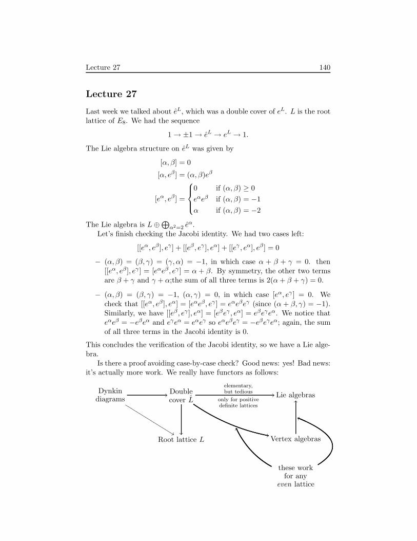
Lecture 27 140
Lecture 27
Last week we talked about eL, which was a double cover of eL. L is the rootlattice of E8. We had the sequence
1 → ±1 → eL → eL → 1.
The Lie algebra structure on eL was given by
[α, β] = 0
[α, eβ ] = (α, β)eβ
[eα, eβ ] =
0 if (α, β) ≥ 0
eαeβ if (α, β) = −1
α if (α, β) = −2
The Lie algebra is L⊕⊕α2=2 eα.
Let’s finish checking the Jacobi identity. We had two cases left:
[[eα, eβ ], eγ ] + [[eβ , eγ ], eα] + [[eγ , eα], eβ ] = 0
− (α, β) = (β, γ) = (γ, α) = −1, in which case α + β + γ = 0. then[[eα, eβ ], eγ ] = [eαeβ, eγ ] = α + β. By symmetry, the other two termsare β + γ and γ + α;the sum of all three terms is 2(α+ β + γ) = 0.
− (α, β) = (β, γ) = −1, (α, γ) = 0, in which case [eα, eγ ] = 0. Wecheck that [[eα, eβ ], eα] = [eαeβ, eγ ] = eαeβeγ (since (α + β, γ) = −1).Similarly, we have [[eβ , eγ ], eα] = [eβeγ , eα] = eβeγeα. We notice thateαeβ = −eβeα and eγeα = eαeγ so eαeβeγ = −eβeγeα; again, the sumof all three terms in the Jacobi identity is 0.
This concludes the verification of the Jacobi identity, so we have a Lie alge-bra.
Is there a proof avoiding case-by-case check? Good news: yes! Bad news:it’s actually more work. We really have functors as follows:
Dynkindiagrams
//
%%KKKKKKKKKKKKKKKKK
Doublecover L
elementary,but tedious
only for positivedefinite lattices
//
,,
Lie algebras
Root lattice L Vertex algebras
OO
these workfor any
even lattice
WW
ii

Lecture 27 141
where L is generated by eαi (the i’s are the dots in your Dynkin diagram),with eαi eαj = (−1)(αi,αj)eαj eαi , and −1 is central of order 2.
Unfortunately, you have to spend several weeks learning vertex algebras.In fact, the construction we did was the vertex algebra approach, with allthe vertex algebras removed. So there is a more general construction whichgives a much larger class of infinite-dimensional Lie algebras.
Now we should study the double cover L, and in particular prove itsexistence. Given a Dynkin diagram, we can construct L as generated by theelements eαi for αi simple roots with the given relations. It is easy to checkthat we get a surjective homomorphism L → L with kernel generated by zwith z2 = 1. What’s a little harder to show is that z 6= 1 (i.e., show thatL 6= L). The easiest way to do it is to use cohomology of groups, but sincewe have such an explicit case, we’ll do it bare hands:Problem: Given Z, H groups with Z abelian, construct central extensions
1 → Z → G→ H → 1
(where Z lands in the center of G). Let G be the set of pairs (z, h), andset the product (z1, h1)(z2, h2) = (z1z2c(h1, h2), h1h2), where c(h1, h2) ∈ Z(c(h1, h2) will be a cocycle in group cohomology). We obviously get a homo-morphism by mapping (z, h) 7→ h. If c(1, h) = c(h, 1) = 1 (normalization),then z 7→ (z, 1) is a homomorphism mapping Z to the center of G. In par-ticular, (1, 1) is the identity. We’ll leave it as an exercise to figure out whatthe inverses are. When is this thing associative? Let’s just write everythingout:
((z1, h1)(z2, h2)
)(z3, h3) = (z1z2z3c(h1, h2)c(h1h2, h3), h1h2h3)
(z1, h1)((z2, h2)(z3, h3)
)= (z1z2z3c(h1, h2h3)c(h2, h3), h1h2h3)
so we must have
c(h1, h2)c(h1h2, h3) = c(h1h2, h3)c(h2, h3).
This identity is actually very easy to satisfy in one particular case: whenc is bimultiplicative: c(h1, h2h3) = c(h1, h2)c(h1, h3) and c(h1h2, h3) =c(h1, h3)c(h2, h3). That is, we have a map H × H → Z. Not all cocyclescome from such maps, but this is the case we care about.
To construct the double cover, let Z = ±1 and H = L (free abelian).If we write H additively, we want c to be a bilinear map L × L → ±1.It is really easy to construct bilinear maps on free abelian groups. Justtake any basis α1, . . . , αn of L, choose c(α1, αj) arbitrarily for each i, j andextend c via bilinearity to L × L. In our case, we want to find a doublecover L satisfying eαeβ = (−1)(α,β)eβ eα where eα is a lift of eα. This just
Lecture 27 142
means that c(α, β) = (−1)(α,β)c(β, α). To satisfy this, just choose c(αi, αj)on the basis αi so that c(αi, αj) = (−1)(αi,αj)c(αj , αi). This is trivial todo as (−1)(αi,αi) = 1. Notice that this uses the fact that the lattice is even.There is no canonical way to choose this 2-cocycle (otherwise, the centralextension would split as a product), but all the different double covers areisomorphic because we can specify L by generators and relations. Thus, wehave constructed L (or rather, verified that the kernel of L → L has order2, not 1).
Let’s now look at lifts of automorphisms of L to L.
Exercise 27.1. Any automorphism of L preserving ( , ) lifts to an auto-morphism of L
There are two special cases:
1. −1 is an automorphism of L, and we want to lift it to L explicitly.First attempt: try sending eα to e−α := (eα)−1, which doesn’t workbecause a 7→ a−1 is not an automorphism on non-abelian groups.
Better: ω : eα 7→ (−1)α2/2(eα)−1 is an automorphism of L. To see
this, check
ω(eα)ω(eβ) = (−1)(α2+β2)/2(eα)−1(eβ)−1
ω(eαeβ) = (−1)(α+β)2/2(eβ)−1(eα)−1
which work out just right
2. If r2 = 2, then α 7→ α − (α, r)r is an automorphism of L (reflection
through r⊥). You can lift this by eα 7→ eα(er)−(α,r) × (−1)((α,r)
2 ). Thisis a homomorphism (check it!) of order (usually) 4!
Remark 27.1. Although automorphisms of L lift to automorphisms ofL, the lift might have larger order.
This construction works for the root lattices of An, Dn, E6, E7, andE8; these are the lattices which are even, positive definite, and gener-ated by vectors of norm 2 (in fact, all such lattices are sums of the givenones). What about Bn, Cn, F4 and G2? The reason the constructiondoesn’t work for these cases is because there are roots of different lengths.These all occur as fixed points of diagram automorphisms of An, Dn andE6. In fact, we have a functor from Dynkin diagrams to Lie algebras, soand automorphism of the diagram gives an automorphism of the algebra
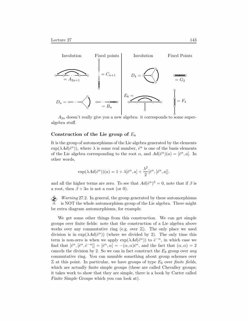
Lecture 27 143
Involution Fixed points Involution Fixed Points
... zz $$|| ""
= A2n+1
...
= Cn+1 D4 = 11
11
//
YY
= G2
//
Dn = ...
????
ZZ
... oo
= Bn
E6 =
zz $$|| ""
= F4
A2n doesn’t really give you a new algebra: it corresponds to some super-algebra stuff.
Construction of the Lie group of E8
It is the group of automorphisms of the Lie algebra generated by the elementsexp(λAd(eα)), where λ is some real number, eα is one of the basis elementsof the Lie algebra corresponding to the root α, and Ad(eα)(a) = [eα, a]. Inother words,
exp(λAd(eα))(a) = 1 + λ[eα, a] +λ2
2[eα, [eα, a]].
and all the higher terms are zero. To see that Ad(eα)3 = 0, note that if β isa root, then β + 3α is not a root (or 0).
Warning 27.2. In general, the group generated by these automorphismsis NOT the whole automorphism group of the Lie algebra. There might
be extra diagram automorphisms, for example.
We get some other things from this construction. We can get simplegroups over finite fields: note that the construction of a Lie algebra aboveworks over any commutative ring (e.g. over Z). The only place we useddivision is in exp(λAd(eα)) (where we divided by 2). The only time thisterm is non-zero is when we apply exp(λAd(eα)) to e−α, in which case wefind that [eα, [eα, e−α]] = [eα, α] = −(α,α)eα, and the fact that (α,α) = 2cancels the division by 2. So we can in fact construct the E8 group over anycommutative ring. You can mumble something about group schemes overZ at this point. In particular, we have groups of type E8 over finite fields,which are actually finite simple groups (these are called Chevalley groups;it takes work to show that they are simple, there is a book by Carter calledFinite Simple Groups which you can look at).

Lecture 27 144
Real forms
So we’ve constructed the Lie group and Lie algebra of type E8. There arein fact several different groups of type E8. There is one complex Lie algebraof type E8, which corresponds to several different real Lie algebras of typeE8.
Let’s look at some smaller groups:
Example 27.3. sl2(R) =(a bc d
)with a, b, c, d real a + d = 0; this is not
compact. On the other hand, su2(R) =(a bc d
)with d = −a imaginary
b = −c, is compact. These have the same Lie algebra over C.
Let’s look at what happens for E8. In general, suppose L is a Lie algebrawith complexification L⊗ C. How can we find another Lie algebra M withthe same complexification? L⊗C has an anti-linear involution ωL : l⊗ z 7→l ⊗ z. Similarly, it has an anti-linear involution ωM . Notice that ωLωM isa linear involution of L⊗C. Conversely, if we know this involution, we canreconstruct M from it. Given an involution ω of L ⊗ C, we can get M asthe fixed points of the map a 7→ ωLω(a)“=” ω(a). Another way is to putL = L+ ⊕ L−, which are the +1 and −1 eigenspaces, then M = L+ ⊕ iL−.
Thus, to find other real forms, we have to study the involutions of thecomplexification of L. The exact relation is kind of subtle, but this is a goodway to go.
Example 27.4. Let L = sl2(R). It has an involution ω(m) = −mT . su2(R)is the set of fixed points of the involution ω times complex conjugation onsl2(C), by definition.
So to construct real forms of E8, we want some involutions of the Liealgebra E8 which we constructed. What involutions do we know about?There are two obvious ways to construct involutions:
1. Lift −1 on L to eα 7→ (−1)α2/2(eα)−1, which induces an involution on
the Lie algebra.
2. Take β ∈ L/2L, and look at the involution eα 7→ (−1)(α,β)eα.
(2) gives nothing new ... you get the Lie algebra you started with. (1) onlygives you one real form. To get all real forms, you multiply these two kindsof involutions together.
Recall that L/2L has 3 orbits under the action of the Weyl group, of size1, 120, and 135. These will correspond to the three real forms of E8. Howdo we distinguish different real forms? The answer was found by Cartan:look at the signature of an invariant quadratic form on the Lie algebra!
A bilinear form ( , ) on a Lie algebra is called invariant if ([a, b], c) +(b[a, c]) = 0 for all a, b, c. This is called invariant because it corresponds to

Lecture 27 145
the form being invariant under the corresponding group action. Now we canconstruct an invariant bilinear form on E8 as follows:
1. (α, β)in the Lie algebra = (α, β)in the lattice
2. (eα, (eα)−1) = 1
3. (a, b) = 0 if a and b are in root spaces α and β with α+ β 6= 0.
This gives an invariant inner product on E8, which you prove by case-by-casecheck
Exercise 27.2. do these checks
Next time, we’ll use this to produce bilinear forms on all the real formsand then we’ll calculate the signatures.
Lecture 28 146
Lecture 28
Last time, we constructed a Lie algebra of type E8, which was L ⊕⊕ eα,where L is the root lattice and α2 = 2. This gives a double cover of the rootlattice:
1 → ±1 → eL → eL → 1.
We had a lift for ω(α) = −α, given by ω(eα) = (−1)(α2/2)(eα)−1. So ω
becomes an automorphism of order 2 on the Lie algebra. eα 7→ (−1)(α,β)eα
is also an automorphism of the Lie algebra.Suppose σ is an automorphism of order 2 of the real Lie algebra L =
L+ + L− (eigenspaces of σ). We saw that you can construct another realform given by L+ + iL−. Thus, we have a map from conjugacy classes ofautomorphisms with σ2 = 1 to real forms of L. This is not in general inisomorphism.
Today we’ll construct some more real forms of E8. E8 has an invari-ant symmetric bilinear form (eα, (eα)−1) = 1, (α, β) = (β, α). The form isunique up to multiplication by a constant since E8 is an irreducible repre-sentation of E8. So the absolute value of the signature is an invariant of theLie algebra.
For the split form of E8, what is the signature of the invariant bilinearform (the split form is the one we just constructed)? On the Cartan subal-gebra L, ( , ) is positive definite, so we get +8 contribution to the signature.On eα, (eα)−1, the form is
(0 11 0
), so it has signature 0 · 120. Thus, the
signature is 8. So if we find any real form with a different signature, we’llhave found a new Lie algebra.
Let’s first try involutions eα 7→ (−1)(α,β)eα. But this doesn’t change thesignature. L is still positive definite, and you still have
(0 11 0
)or(
0 −1−1 0
)on
the other parts. These Lie algebras actually turn out to be isomorphic towhat we started with (though we haven’t shown that they are isomorphic).
Now try ω : eα 7→ (−1)α2/2(eα)−1, α 7→ −α. What is the signature of the
form? Let’s write down the + and − eigenspaces of ω. The + eigenspacewill be spanned by eα − e−α, and these vectors have norm −2 and areorthogonal. The − eigenspace will be spanned by eα + e−α and L, whichhave norm 2 and are orthogonal, and L is positive definite. What is the Liealgebra corresponding to the involution ω? It will be spanned by eα − e−α
where α2 = 2 (norm −2), and i(eα + e−α) (norm −2), and iL (which is nownegative definite). So the bilinear form is negative definite, with signature−248(6= ±8).
With some more work, you can actually show that this is the Lie algebraof the compact form of E8. This is because the automorphism group of E8
preserves the invariant bilinear form, so it is contained in O0,248(R), whichis compact.

Lecture 28 147
Now let’s look at involutions of the form eα 7→ (−1)(α,β)ω(eα). Noticethat ω commutes with eα 7→ (−1)(α,β)eα. The β’s in (α, β) correspond toL/2L modulo the action of the Weyl group W (E8). Remember this hasthree orbits, with 1 norm 0 vector, 120 norm 2 vectors, and 135 norm 4vectors. The norm 0 vector gives us the compact form. Let’s look at theother cases and see what we get.
Suppose V has a negative definite symmetric inner product ( , ), andsuppose σ is an involution of V = V+ ⊕ V− (eigenspaces of σ). What isthe signature of the invariant inner product on V+ ⊕ iV−? On V+, it isnegative definite, and on iV− it is positive definite. Thus, the signature isdimV− − dimV+ = −tr(σ). So we want to work out the traces of theseinvolutions.
Given some β ∈ L/2L, what is tr(eα 7→ (−1)(α,β)eα)? If β = 0, thetraces is obviously 248 because we just have the identity map. If β2 = 2, weneed to figure how many roots have a given inner product with β. Recallthat this was determined before:
(α, β) # of roots α with given inner product eigenvalue
2 1 11 56 -10 126 1-1 56 -1-2 1 1
Thus, the trace is 1 − 56 + 126 − 56 + 1 + 8 = 24 (the 8 is from the Cartansubalgebra). So the signature of the corresponding form on the Lie algebrais −24. We’ve found a third Lie algebra.
If we also look at the case when β2 = 4, what happens? How many αwith α2 = 2 and with given (α, β) are there? In this case, we have:
(α, β) # of roots α with given inner product eigenvalue
2 14 11 64 -10 84 1-1 64 -1-2 14 1
The trace will be 14−64+84−64+14+8 = −8. This is just the split formagain.
Summary: We’ve found 3 forms of E8, corresponding to 3 classes inL/2L, with signatures 8, −24, −248, corresponding to involutions eα 7→(−1)(α,β)e−α of the compact form. If L is the compact form of a simpleLie algebra, then Cartan showed that the other forms correspond exactly tothe conjugacy classes of involutions in the automorphism group of L (this
Lecture 28 148
doesn’t work if you don’t start with the compact form — so always startwith the compact form).
In fact, these three are the only forms of E8, but we won’t prove that.
Working with simple Lie groups
As an example of how to work with simple Lie groups, we will look at thegeneral question: Given a simple Lie group, what is its homotopy type?Answer: G has a unique conjugacy class of maximal compact subgroups K,and G is homotopy equivalent to K.
Proof for GLn(R). First pretend GLn(R) is simple, even though it isn’t;whatever. There is an obvious compact subgroup: On(R). Suppose Kis any compact subgroup of GLn(R). Choose any positive definite form( , ) on Rn. This will probably not be invariant under K, but since Kis compact, we can average it over K get one that is: define a new form(a, b)new =
∫
K(ka, kb) dk. This gives an invariant positive definite bilinearform (since integral of something positive definite is positive definite). Thus,any compact subgroup preserves some positive definite form. But the sub-group fixing some positive definite bilinear form is conjugate to a subgroupof On(R) (to see this, diagonalize the form). SoK is contained in a conjugateof On(R).
Next we want to show that G = GLn(R) is homotopy equivalent toOn(R) = K. We will show that G = KAN , where K is On, A is alldiagonal matrices with positive coefficients, and N is matrices which areupper triangular with 1s on the diagonal. This is the Iwasawa decomposition.In general, we get K compact, A semi-simple abelian, and N is unipotent.The proof of this you saw before was called the Grahm-Schmidt process fororthonormalizing a basis. Suppose v1, . . . , vn is any basis for Rn.
1. Make it orthogonal by subtracting some stuff, you’ll get v1, v2 − ∗v1,v3 − ∗v2 − ∗v1, . . . .
2. Normalize by multiplying each basis vector so that it has norm 1. Nowwe have an orthonormal basis.
This is just another way to say that GLn can be written as KAN . Makingthings orthogonal is just multiplying by something in N , and normalizingis just multiplication by some diagonal matrix with positive entries. Anorthonormal basis is an element of On. Tada! This decomposition is just atopological one, not a decomposition as groups. Uniqueness is easy to check.
Now we can get at the homotopy type of GLn. N ∼= Rn(n−1)/2, andA ∼= (R+)n, which are contractible. Thus, GLn(R) has the same homotopytype as On(R), its maximal compact subgroup.

Lecture 28 149
If you wanted to know π1(GL3(R)), you could calculate π1(O3(R)) ∼=Z/2Z, so GL3(R) has a double cover. Nobody has shown you this doublecover because it is not algebraic.
Example 28.1. Let’s go back to various forms of E8 and figure out (guess)the fundamental groups. We need to know the maximal compact subgroups.
1. One of them is easy: the compact form is its own maximal compactsubgroup. What is the fundamental group? Remember or quote thefact that for compact simple groups, π1
∼= weight latticeroot lattice , which is 1. So
this form is simply connected.
2. β2 = 2 case (signature −24). Recall that there were 1, 56, 126, 56, and1 roots α with (α, β) = 2, 1, 0,−1, and -2 respectively, and there areanother 8 dimensions for the Cartan subalgebra. On the 1, 126, 1, 8parts, the form is negative definite. The sum of these root spacesgives a Lie algebra of type E7A1 with a negative definite bilinear form(the 126 gives you the roots of an E7, and the 1s are the roots of anA1). So it a reasonable guess that the maximal compact subgroup hassomething to do with E7A1. E7 and A1 are not simply connected: thecompact form of E7 has π1 = Z/2 and the compact form of A1 also hasπ1 = Z/2. So the universal cover of E7A1 has center (Z/2)2. Whichpart of this acts trivially on E8? We look at the E8 Lie algebra asa representation of E7 × A1. You can read off how it splits form thepicture above: E8
∼= E7 ⊕A1 ⊕ 56⊗ 2, where 56 and 2 are irreducible,and the centers of E7 and A1 both act as −1 on them. So the maximalcompact subgroup of this form of E8 is the simply connected compactform of E7 ×A1/(−1,−1). This means that π1(E8) is the same as π1
of the compact subgroup, which is (Z/2)2/(−1,−1) ∼= Z/2. So thissimple group has a nontrivial double cover (which is non-algebraic).
3. For the other (split) form of E8 with signature 8, the maximal compactsubgroup is Spin16(R)/(Z/2), and π1(E8) is Z/2.
You can compute any other homotopy invariants with this method.
Let’s look at the 56-dimensional representation of E7 in more detail. Wehad the picture
(α, β) # of α’s
2 11 560 126-1 56-2 1

Lecture 28 150
The Lie algebra E7 fixes these 5 spaces of E8 of dimensions 1, 56, 126 +8, 56, 1. From this we can get some representations of E7. The 126+8 splitsas 1 + (126 + 7). But we also get a 56-dimensional representation of E7.Let’s show that this is actually an irreducible representation. Recall that incalculating W (E8), we showed that W (E7) acts transitively on this set of56 roots of E8, which can be considered as weights of E7.
An irreducible representation is called minuscule if the Weyl group actstransitively on the weights. This kind of representation is particularly easyto work with. It is really easy to work out the character for example: justtranslate the 1 at the highest weight around, so every weight has multiplicity1.
So the 56-dimensional representation of E7 must actually be the irre-ducible representation with whatever highest weight corresponds to one ofthe vectors.
Every possible simple Lie group
We will construct them as follows: Take an involution σ of the compactform L = L+ + L− of the Lie algebra, and form L+ + iL−. The way weconstructed these was to first construct An, Dn, E6, and E7 as for E8. Thenconstruct the involution ω : eα 7→ −e−α. We get Bn, Cn, F4, and G2 asfixed points of the involution ω.
Kac classified all automorphisms of finite order of any compact simpleLie group. The method we’ll use to classify involutions is extracted from hismethod. We can construct lots of involutions as follows:
1. Take any Dynkin diagram, say E8, and select some of its vertices,corresponding to simple roots. Get an involution by taking eα 7→ ±eαwhere the sign depends on whether α is one of the simple roots we’veselected. However, this is not a great method. For one thing, you geta lot of repeats (recall that there are only 3, and we’ve found 28 thisway).
'!&"%#$1 '!&"%#$1
'!&"%#$ 1
2. Take any diagram automorphism of order 2, such as
zz $$ !!
This gives you more involutions.

Lecture 28 151
Next time, we’ll see how to cut down this set of involutions.

Lecture 29 152
Lecture 29
Split form of Lie algebra (we did this for An, Dn, E6, E7, E8): A =⊕eα⊕L.
Compact form A+ + iA−, where A± eigenspaces of ω : eα 7→ (−1)α2/2e−α.
We talked about other involutions of the compact form. You get all theother forms this way.
The idea now is to find ALL real simple Lie algebras by listing all invo-lutions of the compact form. We will construct all of them, but we won’tprove that we have all of them.
We’ll use Kac’s method for classifying all automorphisms of order N ofa compact Lie algebra (and we’ll only use the case N = 2). First let’s lookat inner automorphisms. Write down the AFFINE Dynkin diagram
2
4
6 3
5
4
3
2
1−highest weight =
Choose ni with∑nimi = N where the mi are the numbers on the diagram.
We have an automorphism eαj 7→ e2πinj/Neαj induces an automorphism oforder dividing N . This is obvious. The point of Kac’s theorem is thatall inner automorphisms of order dividing N are obtained this way andare conjugate if and only if they are conjugate by an automorphism of theDynkin diagram. We won’t actually prove Kac’s theorem because we justwant to get a bunch of examples. See [Kac90] or [Hel01].
Example 29.1. Real forms of E8. We’ve already found three, and it tookus a long time. We can now do it fast. We need to solve
∑nimi = 2 where
ni ≥ 0; there are only a few possibilities:∑nimi = 2 # of ways how to do it maximal compact
subgroup K
2 × 1 one way
× E8 (compact form)
1 × 2 two ways
× A1E7
×
D8 (split form)1 × 1 + 1 × 1 no ways
The points NOT crossed off form the Dynkin diagram of the maximal com-pact subgroup. Thus, by just looking at the diagram, we can see what allthe real forms are!
Example 29.2. Let’s do E7. Write down the affine diagram:
1 2 3 4
2
3 2 1
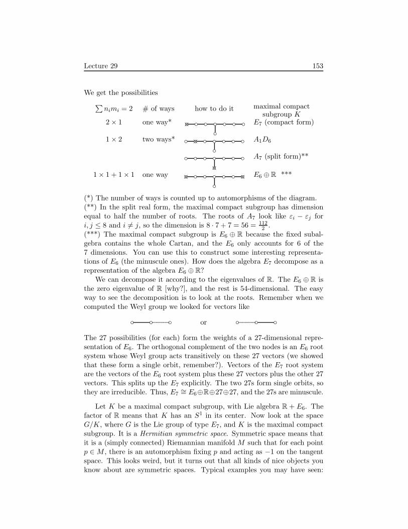
Lecture 29 153
We get the possibilities
∑nimi = 2 # of ways how to do it maximal compact
subgroup K2 × 1 one way* ×
E7 (compact form)
1 × 2 two ways* ×
A1D6
×
A7 (split form)**
1 × 1 + 1 × 1 one way ×
× E6 ⊕ R ***
(*) The number of ways is counted up to automorphisms of the diagram.(**) In the split real form, the maximal compact subgroup has dimensionequal to half the number of roots. The roots of A7 look like εi − εj fori, j ≤ 8 and i 6= j, so the dimension is 8 · 7 + 7 = 56 = 112
2 .(***) The maximal compact subgroup is E6 ⊕ R because the fixed subal-gebra contains the whole Cartan, and the E6 only accounts for 6 of the7 dimensions. You can use this to construct some interesting representa-tions of E6 (the minuscule ones). How does the algebra E7 decompose as arepresentation of the algebra E6 ⊕ R?
We can decompose it according to the eigenvalues of R. The E6 ⊕ R isthe zero eigenvalue of R [why?], and the rest is 54-dimensional. The easyway to see the decomposition is to look at the roots. Remember when wecomputed the Weyl group we looked for vectors like
or
The 27 possibilities (for each) form the weights of a 27-dimensional repre-sentation of E6. The orthogonal complement of the two nodes is an E6 rootsystem whose Weyl group acts transitively on these 27 vectors (we showedthat these form a single orbit, remember?). Vectors of the E7 root systemare the vectors of the E6 root system plus these 27 vectors plus the other 27vectors. This splits up the E7 explicitly. The two 27s form single orbits, sothey are irreducible. Thus, E7
∼= E6⊕R⊕27⊕27, and the 27s are minuscule.
Let K be a maximal compact subgroup, with Lie algebra R + E6. Thefactor of R means that K has an S1 in its center. Now look at the spaceG/K, where G is the Lie group of type E7, and K is the maximal compactsubgroup. It is a Hermitian symmetric space. Symmetric space means thatit is a (simply connected) Riemannian manifold M such that for each pointp ∈ M , there is an automorphism fixing p and acting as −1 on the tangentspace. This looks weird, but it turns out that all kinds of nice objects youknow about are symmetric spaces. Typical examples you may have seen:
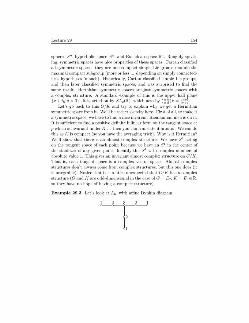
Lecture 29 154
spheres Sn, hyperbolic space Hn, and Euclidean space Rn. Roughly speak-ing, symmetric spaces have nice properties of these spaces. Cartan classifiedall symmetric spaces: they are non-compact simple Lie groups modulo themaximal compact subgroup (more or less ... depending on simply connected-ness hypotheses ’n such). Historically, Cartan classified simple Lie groups,and then later classified symmetric spaces, and was surprised to find thesame result. Hermitian symmetric spaces are just symmetric spaces witha complex structure. A standard example of this is the upper half planex+ iy|y > 0. It is acted on by SL2(R), which acts by
(a bc d
)τ = aτ+b
cτ+d .Let’s go back to this G/K and try to explain why we get a Hermitian
symmetric space from it. We’ll be rather sketchy here. First of all, to make ita symmetric space, we have to find a nice invariant Riemannian metric on it.It is sufficient to find a positive definite bilinear form on the tangent space atp which is invariant underK ... then you can translate it around. We can dothis as K is compact (so you have the averaging trick). Why is it Hermitian?We’ll show that there is an almost complex structure. We have S1 actingon the tangent space of each point because we have an S1 in the center ofthe stabilizer of any given point. Identify this S1 with complex numbers ofabsolute value 1. This gives an invariant almost complex structure on G/K.That is, each tangent space is a complex vector space. Almost complexstructures don’t always come from complex structures, but this one does (itis integrable). Notice that it is a little unexpected that G/K has a complexstructure (G and K are odd-dimensional in the case of G = E7, K = E6⊕R,so they have no hope of having a complex structure).
Example 29.3. Let’s look at E6, with affine Dynkin diagram
1 2 3
2
1
2 1

Lecture 29 155
We get the possibilities∑nimi = 2 # of ways how to do it maximal compact
subgroup K2 × 1 one way
×
E6 (compact form)
1 × 2 one way ×
A1A5
1 × 1 + 1 × 1 one way × ×
D5 ⊕ R
In the last one, the maximal compact subalgebra is D5 ⊕R. Just as before,we get a Hermitian symmetric space. Let’s compute its dimension (overC). The dimension will be the dimension of E6 minus the dimension ofD5 ⊕ R, all divided by 2 (because we want complex dimension), which is(78 − 46)/2 = 16.
So we have found two non-compact simply connected Hermitian sym-metric spaces of dimensions 16 and 27. These are the only “exceptional”cases; all the others fall into infinite families!
There are also some OUTER automorphisms of E6 coming from thediagram automorphism
σ
−→
The fixed point subalgebra has Dynkin diagram obtained by folding the E6
on itself. This is the F4 Dynkin diagram. The fixed points of E6 under thediagram automorphism is an F4 Lie algebra. So we get a real form of E6 withmaximal compact subgroup F4. This is probably the easiest way to constructF4, by the way. Moreover, we can decompose E6 as a representation of F4.dimE6 = 78 and dimF4 = 52, so E6 = F4 ⊕ 26, where 26 turns out to beirreducible (the smallest non-trivial representation of F4 ... the only oneanybody actually works with). The roots of F4 look like (. . . ,±1,±1 . . . )(24 of these) and (±1
2 · · · ± 12) (16 of these), and (. . . ,±1 . . . ) (8 of them) ...
the last two types are in the same orbit of the Weyl group.
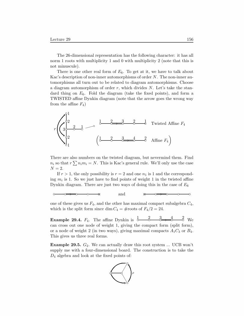
Lecture 29 156
The 26-dimensional representation has the following character: it has allnorm 1 roots with multiplicity 1 and 0 with multiplicity 2 (note that this isnot minuscule).
There is one other real form of E6. To get at it, we have to talk aboutKac’s description of non-inner automorphisms of orderN . The non-inner au-tomorphisms all turn out to be related to diagram automorphisms. Choosea diagram automorphism of order r, which divides N . Let’s take the stan-dard thing on E6. Fold the diagram (take the fixed points), and form aTWISTED affine Dynkin diagram (note that the arrow goes the wrong wayfrom the affine F4)
1 2
3 2 1 2 1
>>
r
$$
:: 1 2 3 // 2 1 Twisted Affine F4
1(
2 3 4 // 2Affine F4
)
33ggggg
There are also numbers on the twisted diagram, but nevermind them. Findni so that r
∑nimi = N . This is Kac’s general rule. We’ll only use the case
N = 2.If r > 1, the only possibility is r = 2 and one n1 is 1 and the correspond-
ing mi is 1. So we just have to find points of weight 1 in the twisted affineDynkin diagram. There are just two ways of doing this in the case of E6
// × and × //
one of these gives us F4, and the other has maximal compact subalgebra C4,which is the split form since dimC4 = #roots of F4/2 = 24.
Example 29.4. F4. The affine Dynkin is1 2 3 4 // 2 We
can cross out one node of weight 1, giving the compact form (split form),or a node of weight 2 (in two ways), giving maximal compacts A1C3 or B4.This gives us three real forms.
Example 29.5. G2. We can actually draw this root system ... UCB won’tsupply me with a four-dimensional board. The construction is to take theD4 algebra and look at the fixed points of:
11
111
00
ρ
ZZ

Lecture 29 157
We want to find the fixed point subalgebra.Fixed points on Cartan subalgebra: ρ fixes a two-dimensional space, and
has 1-dimensional eigenspaces corresponding to ω and ω, where ω3 = 1. The2-dimensional space will be the Cartan of G2.
Positive roots of D4 as linear combinations of simple roots (not funda-mental weights):
01
0
0
111 00
1
0
111 00
0
1
111
gf ed
`a bc10
0
0
111
gf ed
`a bc
11
0
0
111 10
1
0
111 10
0
1
111
gf ed
`a bc11
1
1
111
gf ed
`a bc
11
1
0
111 10
1
1
111 11
0
1
111
gf ed
`a bc21
1
1
111
gf ed
`a bc
︸ ︷︷ ︸
projections of norm 2/3︸ ︷︷ ︸
projections of norm 2
There are six orbits under ρ, grouped above. It obviously acts on the nega-tive roots in exactly the same way. What we have is a root system with sixroots of norm 2 and six roots of norm 2/3. Thus, the root system is G2:
2• 1•
1•1•
1 •
1•
1•
1•
1
• 1•
11111111111111111
1•1•
1
1111
1111
1111
1111
1
•
One of the only root systems to appear on a country’s national flag. Now
let’s work out the real forms. Look at the affine: 1 2 3 // . we can
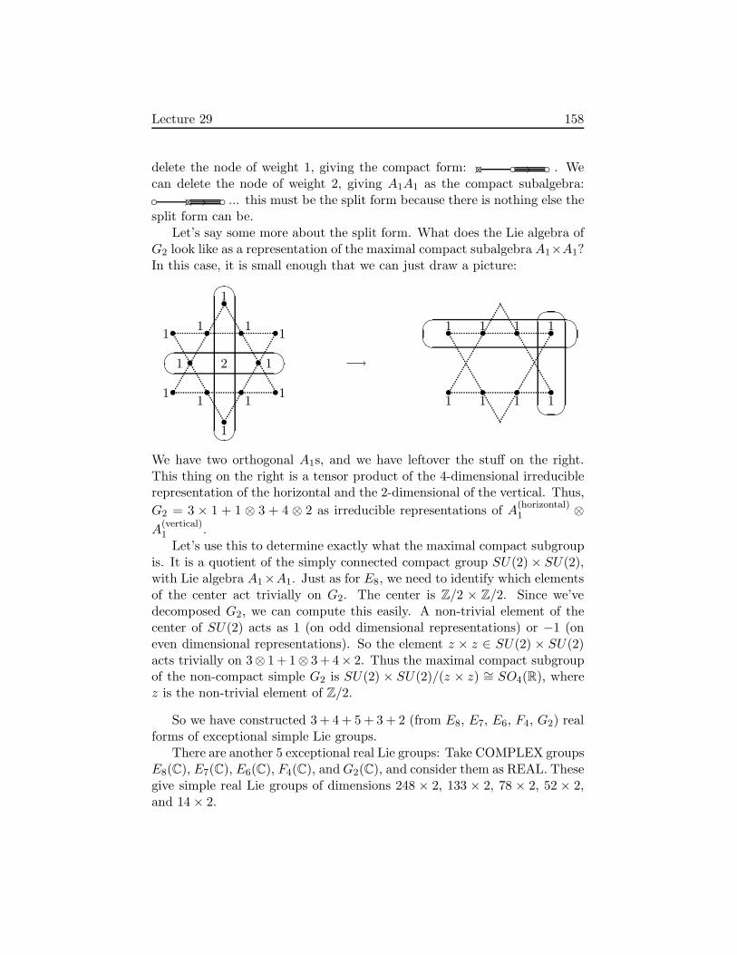
Lecture 29 158
delete the node of weight 1, giving the compact form: × // . Wecan delete the node of weight 2, giving A1A1 as the compact subalgebra: × // ... this must be the split form because there is nothing else thesplit form can be.
Let’s say some more about the split form. What does the Lie algebra ofG2 look like as a representation of the maximal compact subalgebra A1×A1?In this case, it is small enough that we can just draw a picture:
2 1•
1•1•
1 •
1•
1•
1•
1• 1•
1•1•
1•
?> =<89 :;
?> =<
89 :;
−→
1•1•
1•
1•
1•
1•
1•1•?> =<89 :;?> =<
89 :;
We have two orthogonal A1s, and we have leftover the stuff on the right.This thing on the right is a tensor product of the 4-dimensional irreduciblerepresentation of the horizontal and the 2-dimensional of the vertical. Thus,
G2 = 3 × 1 + 1 ⊗ 3 + 4 ⊗ 2 as irreducible representations of A(horizontal)1 ⊗
A(vertical)1 .
Let’s use this to determine exactly what the maximal compact subgroupis. It is a quotient of the simply connected compact group SU(2) × SU(2),with Lie algebra A1×A1. Just as for E8, we need to identify which elementsof the center act trivially on G2. The center is Z/2 × Z/2. Since we’vedecomposed G2, we can compute this easily. A non-trivial element of thecenter of SU(2) acts as 1 (on odd dimensional representations) or −1 (oneven dimensional representations). So the element z × z ∈ SU(2) × SU(2)acts trivially on 3⊗ 1 + 1⊗ 3 + 4× 2. Thus the maximal compact subgroupof the non-compact simple G2 is SU(2) × SU(2)/(z × z) ∼= SO4(R), wherez is the non-trivial element of Z/2.
So we have constructed 3 + 4 + 5 + 3 + 2 (from E8, E7, E6, F4, G2) realforms of exceptional simple Lie groups.
There are another 5 exceptional real Lie groups: Take COMPLEX groupsE8(C), E7(C), E6(C), F4(C), andG2(C), and consider them as REAL. Thesegive simple real Lie groups of dimensions 248 × 2, 133 × 2, 78 × 2, 52 × 2,and 14 × 2.
Lecture 30 - Irreducible unitary representations of SL2(R) 159
Lecture 30 - Irreducible unitary representations of
SL2(R)
SL2(R) is non-compact. For compact Lie groups, all unitary representationsare finite dimensional, and are all known well. For non-compact groups, thetheory is much more complicated. Before doing the infinite-dimensionalrepresentations, we’ll review finite-dimensional (usually not unitary) repre-sentations of SL2(R).
Finite dimensional representations
Finite-dimensional complex representations of the following are much thesame: SL2(R), sl2R, sl2C [branch SL2(C) as a complex Lie group] (as acomplex Lie algebra), su2R (as a real Lie algebra), and SU2 (as a real Liegroup). This is because finite-dimensional representations of a simply con-nected Lie group are in bijection with representations of the Lie algebra.Complex representations of a REAL Lie algebra L correspond to complexrepresentations of its complexification L⊗C considered as a COMPLEX Liealgebra.
Note: Representations of a COMPLEX Lie algebra L ⊗ C are not thesame as representations of the REAL Lie algebra L⊗ C ∼= L+ L. The rep-resentations of the real Lie algebra correspond roughly to (reps of L)⊗(repsof L).
Strictly speaking, SL2(R) is not simply connected, which is not impor-tant for finite-dimensional representations.
Recall the main results for representations of SU2:
1. For each positive integer n, there is one irreducible representation ofdimension n.
2. The representations are completely reducible (every representation isa sum of irreducible ones). This is perhaps the most important fact.
The finite-dimensional representation theory of SU2 is EASIER thanthe representation theory of the ABELIAN Lie group R2, and that isbecause representations of SU2 are completely reducible.
For example, it is very difficult to classify pairs of commuting nilpotentmatrices.
Completely reducible representations:
1. Complex representations of finite groups.
2. Representations of compact groups (Weyl character formula)
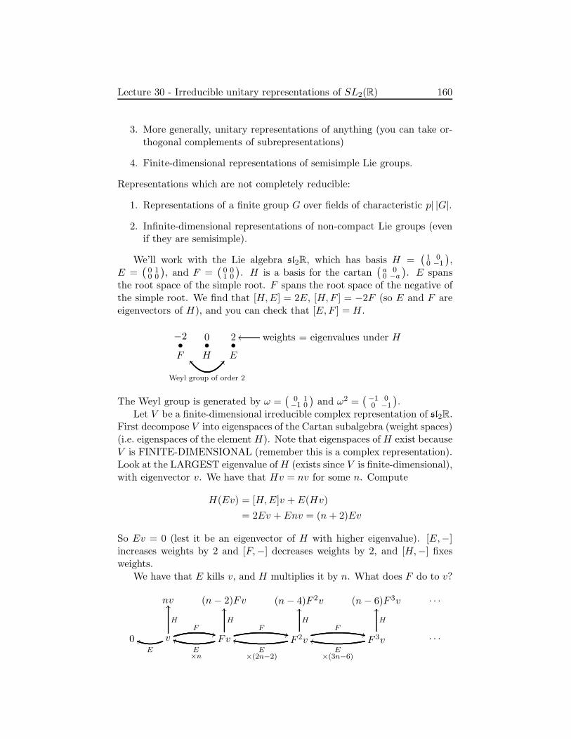
Lecture 30 - Irreducible unitary representations of SL2(R) 160
3. More generally, unitary representations of anything (you can take or-thogonal complements of subrepresentations)
4. Finite-dimensional representations of semisimple Lie groups.
Representations which are not completely reducible:
1. Representations of a finite group G over fields of characteristic p| |G|.
2. Infinite-dimensional representations of non-compact Lie groups (evenif they are semisimple).
We’ll work with the Lie algebra sl2R, which has basis H =(
1 00 −1
),
E =(
0 10 0
), and F =
(0 01 0
). H is a basis for the cartan
(a 00 −a
). E spans
the root space of the simple root. F spans the root space of the negative ofthe simple root. We find that [H,E] = 2E, [H,F ] = −2F (so E and F areeigenvectors of H), and you can check that [E,F ] = H.
0
H•
−2•F
2•E
BB
Weyl group of order 2
[[
weights = eigenvalues under Hoo
The Weyl group is generated by ω =(
0 1−1 0
)and ω2 =
(−1 00 −1
).
Let V be a finite-dimensional irreducible complex representation of sl2R.First decompose V into eigenspaces of the Cartan subalgebra (weight spaces)(i.e. eigenspaces of the element H). Note that eigenspaces ofH exist becauseV is FINITE-DIMENSIONAL (remember this is a complex representation).Look at the LARGEST eigenvalue ofH (exists since V is finite-dimensional),with eigenvector v. We have that Hv = nv for some n. Compute
H(Ev) = [H,E]v + E(Hv)
= 2Ev + Env = (n+ 2)Ev
So Ev = 0 (lest it be an eigenvector of H with higher eigenvalue). [E,−]increases weights by 2 and [F,−] decreases weights by 2, and [H,−] fixesweights.
We have that E kills v, and H multiplies it by n. What does F do to v?
nv (n− 2)Fv (n− 4)F 2v (n− 6)F 3v . . .
0 vE
hh
H
OO
F++Fv
E×n
jj
H
OO
F,,F 2v
E×(2n−2)
kk
H
OO
F,,F 3v
E×(3n−6)
ll
H
OO
. . .

Lecture 30 - Irreducible unitary representations of SL2(R) 161
What is E(Fv)? Well,
EFv = FEv + [E,F ]v
= 0 +Hv = nv
In general, we have
H(F iv) = (n− 2i)F iv
E(F iv) = (ni− i(i− 1))F i−1v
F (F iv) = F i+1v
So the vectors F iv span V because they span an invariant subspace. Thisgives us an infinite number of vectors in distinct eigenspaces of H, and V isfinite-dimensional. Thus, F kv = 0 for some k. Suppose k is the SMALLESTinteger such that F kv = 0. Then
0 = E(F kv) = (nk − k(k − 1))EF k−1v︸ ︷︷ ︸
6=0
So nk − k(k − 1) = 0, and k 6= 0, so n − (k − 1) = 0, so k = n+ 1 . So Vhas a basis consisting of v, Fv, . . . , Fnv. The formulas become a little betterif we use the basis wn = v,wn−2 = Fv,wn−4 = F 2v
2! ,F 3v3! , . . . ,
Fnvn! .
w−6
1
!!
aa
6
w−4
2
!!
aa
5
w−2
3
!!
aa
4
w0
4
__
3
w2
5
__
2
w4
6
__
1
w6
E
F
This says that E(w2) = 5w4 for example. So we’ve found a complete descrip-tion of all finite-dimensional irreducible complex representations of sl2R.This is as explicit as you could possibly want.
These representations all lift to the group SL2(R): SL2(R) acts on ho-mogeneous polynomials of degree n by
(a bc d
)f(x, y) = f(ax + by, cx + dy).
This is an n+ 1-dimensional space, and you can check that the eigenspacesare xiyn−i.
We have implicitly constructed VERMA MODULES. We have a basiswn, wn−2, . . . , wn−2i, . . . with relations H(wn−2i) = (n−2i)wn−2i, Ewn−2i =(n − i + 1)wn−2i+2, and Fwn−2i = (i + 1)wn−2i−2. These are obtained bycopying the formulas from the finite-dimensional case, but allow it to beinfinite-dimensional. This is the universal representation generated by thehighest weight vector wn with eigenvalue n under H (highest weight justmeans E(wn) = 0).
Let’s look at some things that go wrong in infinite dimensions.
Lecture 30 - Irreducible unitary representations of SL2(R) 162
Warning 30.1. Representations corresponding to the Verma modulesdo NOT lift to representations of SL2(R), or even to its universal cover.
The reason: look at the Weyl group (generated by(
0 1−1 0
)) of SL2(R) acting
on 〈H〉; it changes H to −H. It maps eigenspaces with eigenvalue m toeigenvalue −m. But if you look at the Verma module, it has eigenspacesn, n − 2, n − 4, . . . , and this set is obviously not invariant under changingsign. The usual proof that representations of the Lie algebra lifts uses theexponential map of matrices, which doesn’t converge in infinite dimensions.
Remark 30.2. The universal cover SL2(R) of SL2(R), or even the doublecover Mp2(R), has NO faithful finite-dimensional representations.
Proof. Any finite dimensional representation comes from a finite dimen-sional representation of the Lie algebra sl2R. All such finite dimensionalrepresentations factor through SL2(R).
All finite-dimensional representations of SL2(R) are completely reducible.Weyl did this by Weyl’s unitarian trick:
Notice that finite-dimensional representations of SL2(R) are isomorphic(sort of) to finite-dimensional representations of the COMPACT group SU2
(because they have the same complexified Lie algebras. Thus, we just have toshow it for SU2. But representations of ANY compact group are completelyreducible. Reason:
1. All unitary representations are completely reducible (if U ⊆ V , thenV = U ⊕ U⊥).
2. Any representation V of a COMPACT group G can be made unitary:take any unitary form on V (not necessarily invariant under G), andaverage it over G to get an invariant unitary form. We can averagebecause G is compact, so we can integrate any continuous functionover G. This form is positive definite since it is the average of positivedefinite forms (if you try this with non-(positive definite) forms, youmight get zero as a result).
The Casimir operator
Set Ω = 2EF + 2FE +H2 ∈ U(sl2R). The main point is that Ω commuteswith sl2R. You can check this by brute force:
[H,Ω] = 2 ([H,E]F + E[H,F ])︸ ︷︷ ︸
0
+ · · ·
[E,Ω] = 2[E,E]F + 2E[F,E] + 2[E,F ]E
+ 2F [E,E] + [E,H]H +H[E,H] = 0
[F,Ω] = Similar

Lecture 30 - Irreducible unitary representations of SL2(R) 163
Thus, Ω is in the center of U(sl2R). In fact, it generates the center. Thisdoesn’t really explain where Ω comes from.
Remark 30.3. Why does Ω exist? The answer is that it comes from a sym-metric invariant bilinear form on the Lie algebra sl2R given by (E,F ) = 1,(E,E) = (F,F ) = (F,H) = (E,H) = 0, (H,H) = 2. This bilinear form isan invariant map L⊗L→ C, where L = sl2R, which by duality gives an in-variant element in L⊗L, which turns out to be 2E⊗F+2F⊗E+H⊗H. Theinvariance of this element corresponds to Ω being in the center of U(sl2R).
Since Ω is in the center of U(sl2R), it acts on each irreducible represen-tation as multiplication by a constant. We can work out what this constantis for the finite-dimensional representations. Apply Ω to the highest vectorwn:
(2EF + 2FE +HH)wn = (2n + 0 + n2)wn
= (2n + n2)wn
So Ω has eigenvalue 2n+ n2 on the irreducible representation of dimensionn+1. Thus, Ω has DISTINCT eigenvalues on different irreducible represen-tations, so it can be used to separate different irreducible representations.The main use of Ω will be in the next lecture, where we’ll use it to deal withinfinite-dimensional representation.
To finish today’s lecture, let’s look at an application of Ω. We’ll sketch analgebraic argument that the representations of sl2R are completely reducible.Given an exact sequence of representations
0 → U → V →W → 0
we want to find a splitting W → V , so that V = U ⊕W .Step 1: Reduce to the case where W = C. The idea is to look at
0 → HomC(W,U) → HomC(W,V ) → HomC(W,W ) → 0
and HomC(W,W ) has an obvious one-dimensional subspace, so we can geta smaller exact sequence
0 → HomC(W,U) → subspace of HomC(W,V ) → C→ 0
and if we can split this, the original sequence splits.Step 2: Reduce to the case where U is irreducible. This is an easy
induction on the number of irreducible components of U .
Exercise 30.1. Do this.
Lecture 30 - Irreducible unitary representations of SL2(R) 164
Step 3: This is the key step. We have
0 → U → V → C→ 0
with U irreducible. Now apply the Casimir operator Ω. V splits as eigen-values of Ω, so is U⊕C UNLESS U has the same eigenvalue as C (i.e. unlessU = C).
Step 4: We have reduced to
0 → C→ V → C→ 0
which splits because sl2(R) is perfect1 (no homomorphisms to the abelianalgebra
(0 ∗0 0
)).
Next time, in the final lecture, we’ll talk about infinite-dimensional uni-tary representations.
1L is perfect if [L, L] = L

Lecture 31 - Unitary representations of SL2(R) 165
Lecture 31 - Unitary representations of SL2(R)
Last lecture, we found the finite-dimensional (non-unitary) representationsof SL2(R).
Background about infinite-dimensional representations
(of a Lie group G) What is an finite-dimensional representation?
1st guess Banach space acted on by G?
This is no good for some reasons: Look at the action of G on thefunctions on G (by left translation). We could use L2 functions, orL1 or Lp. These are completely different Banach spaces, but they areessentially the same representation.
2nd guess Hilbert space acted on by G? This is sort of okay.
The problem is that finite dimensional representations of SL2(R) areNOT Hilbert space representations, so we are throwing away someinteresting representations.
Solution (Harish-Chandra) Take g to be the Lie algebra of G, and let K be themaximal compact subgroup. If V is an infinite-dimensional represen-tation of G, there is no reason why g should act on V .
The simplest example fails. Let R act on L2(R) by left translation.Then the Lie algebra is generated by d
dx (or i ddx) acting on L2(R), butddx of an L2 function is not in L2 in general.
Let V be a Hilbert space. Set Vω to be the K-finite vectors of V ,which are the vectors contained in a finite-dimensional representationof K. The point is that K is compact, so V splits into a Hilbert spacedirect sum finite-dimensional representations of K, at least if V is aHilbert space. Then Vω is a representation of the Lie algebra g, nota representation of G. Vω is a representation of the group K. It isa (g,K)-module, which means that it is acted on by g and K in a“compatible” way, where compatible means that
1. they give the same representations of the Lie algebra of K.
2. k(u)v = k(u(k−1v)) for k ∈ K, u ∈ g, and v ∈ V .
The K-finite vectors of an irreducible unitary representation of G isADMISSIBLE, which means that every representation of K only oc-curs a finite number of times. The GOOD category of representationsis the representations of admissible (g,K)-modules. It turns out thatthis is a really well behaved category.

Lecture 31 - Unitary representations of SL2(R) 166
We want to find the unitary irreducible representations of G. We willdo this in several steps:
1. Classify all irreducible admissible representations of G. This wassolved by Langlands, Harish-Chandra et. al.
2. Find which have hermitian inner products ( , ). This is easy.
3. Find which ones are positive definite. This is VERY HARD. We’llonly do this for the simplest case: SL2(R).
The group SL2(R)
We found some generators (in Lie(SL2(R)) ⊗ C last time: E, F , H, with[H,E] = 2E, [H,F ] = −2F , and [E,F ] = H. We have that H = −i
(0 1−1 0
),
E = 12
(1 ii −1
), and F = 1
2
(1 −i−i −1
). Why not use the old
(1 00 −1
),(
0 10 0
), and
(0 01 0
)?
Because SL2(R) has two different classes of Cartan subgroup:(a 00 a−1
),
spanned by(
1 00 −1
), and
(cos θ sin θ− sin θ cos θ
), spanned by
(0 1−1 0
), and the second
one is COMPACT. The point is that non-compact (abelian) groups neednot have eigenvectors on infinite-dimensional spaces. An eigenvector is thesame as a weight space. The first thing you do is split it into weight spaces,and if your Cartan subgroup is not compact, you can’t get started. We workwith the compact subalgebra so that the weight spaces exist.
Given the representation V , we can write it as some direct sum ofeigenspaces of H, as the Lie group H generates is compact (isomorphicto S1). In the finite-dimensional case, we found a HIGHEST weight, whichgave us complete control over the representation. The trouble is that ininfinite dimensions, there is no reason for the highest weight to exist, andin general they don’t. The highest weight requires a finite number of eigen-values.
A good substituted for the highest weight vector: Look at the Casimiroperator Ω = 2EF +2FE+H2 +1. The key point is that Ω is in the centerof the universal enveloping algebra. As V is assumed admissible, we canconclude that Ω has eigenvectors (because we can find a finite-dimensionalspace acted on by Ω). As V is irreducible and Ω commutes with G, all of Vis an eigenspace of Ω. We’ll see that this gives us about as much informationas a highest weight vector.
Let the eigenvalue of Ω on V be λ2 (the square will make the interestingrepresentations have integral λ; the +1 in Ω is for the same reason).
Suppose v ∈ Vn, where Vn is the space of vectors where H has eigenvaluen. In the finite-dimensional case, we looked at Ev, and saw that HEv =(n+2)Ev. What is FEv? If v was a highest weight vector, we could controlthis. Notice that Ω = 4FE+H2+2H+1 (using [E,F ] = H), and Ωv = λ2v.

Lecture 31 - Unitary representations of SL2(R) 167
This says that 4FEv + n2v + 2nv + v = λ2v. This shows that FEv is amultiple of v.
Now we can draw a picture of what the representation looks like:
· · ·
]]vn−4
]]vn−2
]]vn
]]n2+2n+1−λ2
4
vn+2
]]vn+4
]]· · ·
E
H
F
Thus, Vω is spanned by Vn+2k, where k is an integer. The non-zero elementsamong the Vn+2k are linearly independent as they have different eigenvalues.The only question remaining is whether any of the Vn+2k vanish.
There are four possible shapes for an irreducible representation
– infinite in both directions: · · · %%ee · %%
ee · %%ee · %%
ee · %%ee · · ·
EHF
– a lowest weight, and infinite in the other direction:
· · · %%ee · %%
ee · %%ee · %%
ee · %%ee · E
HF
– a highest weight, and infinite in the other direction:
· %%ee · %%
ee · %%ee · %%
ee · %%ee · · ·
EHF
– we have a highest weight and a lowest weight, in which case it is finite-
dimensional · %%ee · %%
ee · · · %%ee · %%
ee · EHF
We’ll see that all these show up. We also see that an irreducible representa-tion is completely determined once we know λ and some n for which Vn 6= 0.The remaining question is to construct representations with all possible val-ues of λ ∈ C and n ∈ Z. n is an integer because it must be a representationsof the circle.
If n is even, we have
· · ·
ZZ −6
ZZ −4
ZZ −2
ZZ 0
ZZ 2
ZZ 4
ZZ 6
ZZ· · ·
E
H
F
λ−72
λ−52
λ−32
λ−12
λ+12
λ+32
λ+52
λ+72
λ+72
λ+52
λ+32
λ+12
λ−12
λ−32
λ−52
λ−72
It is easy to check that these maps satisfy [E,F ] = H, [H,E] = 2E, and[H,F ] = −2F

Lecture 31 - Unitary representations of SL2(R) 168
Exercise 31.1. Do the case of n odd.
Problem: These may not be irreducible, and we want to decompose theminto irreducible representations. The only way they can fail to be irreducibleif if Evn = 0 of Fvn = 0 for some n (otherwise, from any vector, you cangenerate the whole space). The only ways that can happen is if
n even: λ an odd integern odd: λ an even integer.
What happens in these cases? The easiest thing is probably just to writeout an example.
Example 31.1. Take n even, and λ = 3, so we have
· · ·
ZZ −6
ZZ −4
ZZ −2
ZZ 0
ZZ 2
ZZ 4
ZZ 6
ZZ· · ·
E
H
F
−2 −1 0 1 2 3 4 5
5 4 3 2 1 0 −1 −2
You can just see what the irreducible subrepresentations are ... they areshown in the picture. So V has two irreducible subrepresentations V− andV+, and V/(V− ⊕ V+) is an irreducible 3-dimensional representation.
Example 31.2. If n is even, but λ is negative, say λ = −3, we get
· · ·
ZZ −6
ZZ −4
ZZ −2
ZZ 0
ZZ 2
ZZ 4
ZZ 6
ZZ· · ·
E
H
F
−5 −4 −3 −2 −1 0 1 2
2 1 0 −1 −2 −3 −4 −5
Here we have an irreducible finite-dimensional representation. If you quo-tient out by that subrepresentation, you get V+ ⊕ V−.
Exercise 31.2. Show that for n odd, and λ = 0, V = V+ ⊕ V−.
So we have a complete list of all irreducible admissible representations:
1. if λ 6∈ Z, you get one representation (remember λ ≡ −λ). This is thebi-infinite case.
2. Finite-dimensional representation for each n ≥ 1 (λ = ±n)
3. Discrete series for each λ ∈ Zr0, which is the half infinite case: youget a lowest weight when λ < 0 and a highest weight when λ > 0.

Lecture 31 - Unitary representations of SL2(R) 169
4. two “limits of discrete series” where n is odd and λ = 0.
Which of these can be made into unitary representations? H† = −H, E† =F , and F † = E. If we have a hermitian inner product ( , ), we see that
(vj+2, vj+2) =2
λ+ j + 1(Evj , vj+2)
=2
λ+ j + 1(vj ,−Fvj+2)
= − 2
λ+ j + 1
λ− j − 1
2(vj , vj) > 0
where we fix the sign errors. So we want −λ−1−jλ+j+1 to be real and positive
whenever j, j + 2 are non-zero eigenvectors. So
−(λ− 1 − j)(λ+ 1 + j) = −λ2 + (j + 1)2
should be positive for all j. Conversely, when you have this, blah.This condition is satisfied in the following cases:
1. λ2 ≤ 0. These representations are called PRINCIPAL SERIES repre-sentations. These are all irreducible except when λ = 0 and n is odd, inwhich case it is the sum of two limits of discrete series representations
2. 0 < λ < 1 and j even. These are called COMPLEMENTARY SERIES.They are annoying, and you spend a lot of time trying to show thatthey don’t occur.
3. λ2 = n2 for n ≥ 1 (for some of the irreducible pieces).
If λ = 1, we get
· · ·
ZZ −6
ZZ −4
ZZ −2
ZZ 0
ZZ 2
ZZ 4
ZZ 6
ZZ· · ·
E
H
F
−3 −2 −1 0 1 2 3 4
4 3 2 1 0 −1 −2 −3
We see that we get two discrete series and a 1-dimensional represen-tation, all of which are unitary
For λ = 2 (this is the more generic one), we have
· · ·
ZZ −5
ZZ −3
ZZ −1
ZZ 1
ZZ 3
ZZ 5
ZZ· · ·
E
H
F
−2 −1 0 1 2 3 4
4 3 2 1 0 −1 −2

Lecture 31 - Unitary representations of SL2(R) 170
The middle representation (where (j + 1)2 < λ2 = 4 is NOT unitary,which we already knew. So the DISCRETE SERIES representationsARE unitary, and the FINITE dimensional representations of dimen-sion greater than or equal to 2 are NOT.
Summary: the irreducible unitary representations of SL2(R) are givenby
1. the 1-dimensional representation
2. Discrete series representations for any λ ∈ Zr 0
3. Two limit of discrete series representations for λ = 0
4. Two series of principal series representations:
j even: λ ∈ iR, λ ≥ 0j odd: λ ∈ iR, λ > 0
5. Complementary series: parameterized by λ, with 0 < λ < 1.
The nice stuff that happened for SL2(R) breaks down for more compli-cated Lie groups.
Representations of finite covers of SL2(R) are similar, except j need not
be integral. For example, for the double cover SL2(R) = Mp2(R), 2j ∈ Z.
Exercise 31.3. Find the irreducible unitary representations of Mp2(R).
Solutions to (some) Exercises 171
Solutions to (some) Exercises
Solution 1.1. Yes. Consider µ−1(e) ⊆ G × G. We would like to usethe implicit function theorem to show that there is a function f (which isas smooth as µ) such that (h, g) ∈ µ−1(e) if and only if g = f(h). Thisfunction will be ι. You need to check that for every g, the derivative of leftmultiplication by g at g−1 is non-singular (i.e. that dlg(g
−1) is a non-singularmatrix). This is obvious because we have an inverse, namely dlg−1(e).
Solution 1.2. Just do it.
Solution 4.1. We calculate:
d
dt‖g(t)‖2 = 2〈 d
dtg, g〉
≤ 2
∥∥∥∥
d
dtg
∥∥∥∥‖g‖
≤ 2‖ξ‖‖g‖2.
That is, η(t) := ‖g(t)‖2 satisfies the differential inequality:
d
dtη(t) ≤ ‖ξ‖η(t),
which in turn implies (Gronwall’s inequality) that
η(t) ≤ e2R tt0
‖ξ(s)‖ds
so that
‖g‖ ≤ eR tt0
‖ξ(s)‖ds
≤ C ′|t− t0|
since for |t− t0| sufficiently small, exponentiation is Lipschitz.
Solution 8.2. We would like to compute the coefficients of the product(XaHbY r)(XsHcY d) once it is rewritten in the PBW basis by repeatedlyapplying the relations XY −Y X = εH, HX = XH, and HY = Y H. Checkby induction that
Y rXs =∞∑
n=0
εn(−1)nn!
(r
n
)(s
n
)
Xr−nH lY s−n.
It follows that pI,Jn is zero unless I = (Y, . . . , Y ) and J = (X, . . . ,X), in
which case pI,Jn = (−1)n
n! Hn.

Solutions to (some) Exercises 172
Solution 9.3. We have [a, b]h :=∑∞
n=0 hnmn(a, b), where m0(a, b) = [a, b].
Now we compute
[a, [b, c]h]h = [a,∑
l≥0
hlml(b, c)]h
=∑
l≥0
hl∑
k≥0
hkmk(a,ml(b, c))
=∑
N≥0
hNmk(a,mN−k(b, c)) (N = k + l)
Adding the cyclic permutations and looking at the coefficient of hN , we getthe desired result.
Solution 11.1. Obvious.
Solution 11.2. [G,G] is normal because r[g, h]r−1 = [rgr−1, rhr−1]. To seethat [G,G] is connected, let γgh : [0, 1] → G be a path from g to h and definethe path t 7→ gγ(t)g−1γ(t)−1 in [G,G] from the identity to [g, h]. Since allthe generators of [G,G] are connected to e ∈ G by paths, all of [G,G] isconnected to e.
Now we show that the Lie algebra of [G,G] is Dg. Consider the Liealgebra homomorphism π : g → g/Dg. Since G is simply connected, thislifts to some Lie group homomorphism p : G→ H:
Dg // g π //
exp
g/Dg
exp
[G,G] // Gp
// H ∼= Rn
where H is the simply connected Lie group with Lie algebra g/Dg. Notethat the Lie algebra of the kernel of p must be contained in ker π = Dg.Also, g/Dg is abelian, so H is abelian, so [G,G] is in the kernel of p. Thisshows that Lie([G,G]) ⊆ Dg.
To see that Dg ⊆ Lie([G,G]), assume that g ⊆ gl(V ). Then for X,Y ∈g consider the path γ(t) = exp(X
√t) exp(Y
√t) exp(−X
√t) exp(−Y
√t) in
[G,G]:
γ(t) =
(
1 +X√t+
1
2X2t+ · · ·
)(
1 + Y√t+
1
2Y 2t+ · · ·
)
×(
1 −X√t+
1
2X2t+ · · ·
)(
1 − Y√t+
1
2Y 2t+ · · ·
)
= 1 +√t(X + Y −X − Y )+
t(XY −X2 −XY − Y X − Y 2 +X2 + Y 2) + · · ·= 1 + t[X,Y ] +O(t3/2)

Solutions to (some) Exercises 173
So γ′(0) = [X,Y ]. This shows that [G,G] is a connected component of thekernel of p.
Since [G,G] is a connected component of p−1(0), it is closed in G.
Solution 11.3. Let π : g → g/rad g be the canonical projection, and assumea ∈ g/rad g is solvable. Then Dka = 0 for some k, so Dkπ−1(a) ⊆ rad g.Since rad g is solvable, we have that DNπ−1(a) = 0 for someN . By definitionof rad g, we get that π−1(a) ⊆ rad g, so a = 0 ⊆ g/rad g. Thus, g/rad g issemi-simple.
Solution 12.1. An invariant form B induces a homomorphism g → g∗.Invariance says that this homomorphism is an intertwiner of representationsof g (with the adjoint action on g and the coadjoint action on g∗). Since g issimple, these are both irreducible representations. By Schur’s Lemma, anytwo such homomorphisms must be proportional, so any two invariant formsmust be proportional.
Solution 12.2. Done in class.
Solution 12.3. yuck.
Solution 12.4. The complex for computing cohomology is
0 −→ kd0−−→ Hom(sl2, k)
d1−−→ Hom(Λ2sl2, k)d2−−→ Hom(Λ3sl2, k) −→ 0
c 7−→ dc(x) = −x · c = 0f 7−→ df(x, y) = f([x, y])
α 7→ dα(x, y, z) = α([x, y], z) − α([x, z], y)+α([y, z], x)
We have that ker d1 = k, so H0(sl2, k) = k. The kernel of d1 is zero, as wecomputed in Remark 12.11. Since Hom(sl2, k) and Hom(Λ2sl2, k) are boththree-dimensional, it follows that d1 is surjective, and since the kernel of d2
must contain the image of d1, we know that d2 is the zero map. This tellsus that H1(sl2, k) = 0, H2(sl2, k) = 0, and H3(sl2, k) = Hom(Λ3sl2, k) ∼= k.
Solution 12.5. Let D ∈ Der(g) and let X,Y ∈ g. Then
[D,adX ]Der(g)(Y ) = D([X,Y ]) − [X,D(Y )]
= [D(X), Y ] + [X,D(Y )] − [X,D(Y )]
= adD(X)(Y ).
Solution 13.1. Let x ∈ h, so [x, h] = 0. Since adxn is a polynomial in adx,we get that [xn, h] = 0, so xn ∈ h. Thus, it is enough to show that anynilpotent element in h is zero. We do this using property 4, that the Killing

Solutions to (some) Exercises 174
form is non-degenerate on h. If y ∈ h, then B(xn, y) = tr(adxn ady). h
is abelian by the proposition, so [xn, y] = 0, so adxn commutes with ady.Thus, we can simultaneously upper triangularize adxn and ady. Since adxn
is nilpotent, it follows that tr(adxn ady) = 0. So xn = 0 by non-degeneracyof B.
Solution 13.2. Since ∆ is a finite set in h∗, we can find some h ∈ h so thatα(h) 6= β(h) for distinct roots α and β. Then this h is a regular elementwhich gives the right Cartan subalgebra, and the desired properties followfrom the properties on page 60.
Solution 13.3. If ∆ does not span h∗, then there is some non-zero h ∈ h
such that α(h) = 0 for all α ∈ ∆. This means that all of the eigenvalues ofadh are zero. Since h is semisimple, adh = 0. And since ad is faithful, weget h = 0, proving property 1.
To prove 2, consider the α-string through β. It must be of the formgβ+nα ⊕ gβ+(n−1)α ⊕ · · · ⊕ gβ+mα for some integers n ≥ 0 ≥ m. From thecharacterization of irreducible finite dimensional representations of sl2, weknow that each eigenvalue of Hα is an integer, so β(Hα) = r ∈ Z (since[Hα,Xβ] = β(Hα)Xβ). We also know that the eigenvalues of Hα are sym-metric around zero, so we must have −r = (β + sα)(Hα) for some s forwhich gβ+sα is in the α-string through β. Then we get β(Hα) + sα(Hα) =β(α) + 2s = −r = −β(α), from which we know that s = −β(Hα). Thus,gβ−β(Hα)α 6= 0, so β −
(β(Hα)
)α is a root.
Finally, we prove 3. If α and β = cα are roots, then by property 2, weknow that α(Hβ) = 2/c and β(Hα) = 2c are integers (note thatHβ = Hα/c).It follows that c = ±1
2 ,±1, or ±2. Therefore, it is enough to show that αand 2α cannot both be roots. To see this, consider the α-string through 2α.We have that [Hα,X2α] = 2α(Hα)X2α = 4X2α, so the α-string must havea non-zero element [Yα,X2α] ∈ gα, which is spanned by Xα. But then wewould have that X2α is a multiple of [Xα,Xα] = 0, which is a contradiction.
Solution 14.1. If ∆ is reducible, with ∆ = ∆1 ∪ ∆2, then set hi to be thespan of ∆i, and set gi = hi ⊕
⊕
α∈∆igα (for i = 1, 2). Then we have that
g = g1 ⊕ g2 as a vector space. We must check that g1 is an ideal (the bysymmetry, g2 will also be an ideal). From the relation [gα, gβ] ⊆ gα+β, weknow that it is enough to check that for α ∈ ∆1,
[gα, g−α] ⊆ h1, and (1)
[gα, h2] = 0. (2)
Letting β ∈ ∆2, we have that β([Xα, Yα]) = β(Hα) = 2(α,β)(β,β) = 0 because
∆1 and ∆2 are orthogonal; 1 follows because ∆2 spans the orthogonal com-plement of h1 in h. Similarly, we have [Xα,Hβ] = α(Hβ)Xα = 0; 2 followsbecause the Hβ span h2.
Solutions to (some) Exercises 175
If, conversely, g = g1 ⊕ g2, then since g1 and g2 are ideals, we get thatthe roots coming from g1 are orthogonal to the roots from g2, showing thatthe root system of g is reducible.

References 176
References
[Ada69] J. Frank Adams. Lectures on Lie groups. W. A. Benjamin, Inc.,New York-Amsterdam, 1969.
[Ada96] J. Frank Adams. Lectures on exceptional Lie groups. ChicagoLectures in Mathematics. University of Chicago Press, Chicago,IL, 1996.
[Bor91] Armand Borel. Linear algebraic groups, volume 126 of GraduateTexts in Mathematics. Springer-Verlag, New York, second enlargededition, 1991.
[CSM95] Roger Carter, Graeme Segal, and Ian Macdonald. Lectures onLie groups and Lie algebras, volume 32 of London MathematicalSociety Student Texts. Cambridge University Press, Cambridge,1995.
[FH91] William Fulton and Joe and Harris. Representation theory, volume129 of Graduate Texts in Mathematics. Springer-Verlag, New York,1991. 5, 46
[Fuc50] Dmitry Fuchs. Cohomology of infinite dimensional Lie algebras?I don’t know if this book exists, 2050. 41
[Hat02] Allen Hatcher. Algebraic topology. Cambridge University Press,Cambridge, 2002. 18, 56
[Hel01] Sigurdur Helgason. Differential geometry, Lie groups, and sym-metric spaces, volume 34 of Graduate Studies in Mathematics.American Mathematical Society, Providence, RI, 2001. 152
[Hum78] James E. Humphreys. Introduction to Lie algebras and representa-tion theory, volume 9 of Graduate Texts in Mathematics. Springer-Verlag, New York, 1978. 61
[Kac90] Victor G. Kac. Infinite-dimensional Lie algebras. Cambridge Uni-versity Press, Cambridge, 1990. 152
[Kna02] Anthony W. Knapp. Lie groups beyond an introduction, volume140 of Progress in Mathematics. Birkhauser Boston Inc., Boston,MA, 2002.
[Lan02] Serge Lang. Algebra, volume 211 of Graduate Texts in Mathemat-ics. Springer-Verlag, New York, 2002. 53

References 177
[Lee03] John M. Lee. Introduction to smooth manifolds, volume 218 ofGraduate Texts in Mathematics. Springer-Verlag, New York, 2003.6
[Mon93] Susan Montgomery. Hopf algebras and their actions on rings,volume 82 of CBMS Regional Conference Series in Mathematics.Published for the Conference Board of the Mathematical Sciences,Washington, DC, 1993. 22
[OV90] A. L. Onishchik and E. B. Vinberg. Lie groups and algebraicgroups. Springer Series in Soviet Mathematics. Springer-Verlag,Berlin, 1990.
[Ser87] Jean-Pierre Serre. Complex semisimple Lie algebras. Springer-Verlag, New York, 1987.
[War83] Frank W. Warner. Foundations of differentiable manifolds and Liegroups, volume 94 of Graduate Texts in Mathematics. Springer-Verlag, New York, 1983.
Index 178
Index
adjoint representation, 27Ado’s Theorem, 5α-string, 64antipode, 21
b, 47Baker-Campbell-Hausdorff, 11
bialgebra, 22Borcherds, Richard E., 3, 105–170
Cartan decomposition, 61Cartan subalgebra, 61Cartan’s Criterion, 54
Casimir operator, 55central extension, 43cohomology
of Lie algebras, 37
Complete reducibility, see Weyl’sTheorem
comultiplication, 21coroot, 66counit, 21covering map, 16Coxeter diagram, 71Coxeter group, 66
d, 47Danish, 21deformation
of a Lie algebra, 42deformations
of associative algebras, 32
derived series, 47dual pairing, 23Dynkin diagram, 71
Engel’s Theorem, 48
exponential map, 10
filtered space, 28
gl∞, 44
gln, 4, 47
Heisenberg algebra, 33, 63Hochschild cohomology, 5Hopf Algebras, 21
Hopf ideal, 25
invariant form, 52
Jacobi identity, 4joke, 178Jordan decomposition, 53
absolute, 59, 60
Kac-Moody algebra, 44Killing form, 52
Knutson, Alan, 3Kontsevitch, Maxim, 35
LATEX, 3Lie algebra, 4
of a Lie group, 6Lie algebra cohomology, 37
Lie derivative, 5Lie group, 4Lie ideal, 6Lie’s Theorem, 49
loop algebra, 44loop space, 44lower central series, 47
nilpotent, 47element, 60
one-parameter subgroup, 10
PBW, see Poincare-Birkhoff-WittPoincare-Birkhoff-Witt, 31
rank, 62, 67real form, 4regular element, 60

Index 179
representations, 26Reshetikhin, Nicolai, 3–45root, 61
positive, 69simple, 69
root space, 61root decomposition, 61root system
abstract, 67irreducible, 67
semisimple, 51element, 60
Serganova, Vera, 3, 46–104sl2, 61, 63sl3, 62sln, 60solvable, 47star product, 34
unitary trick, 58universal cover, 17universal enveloping algebra, 24–
32upper triangular, see b
useful facts, 47–48
variety of Lie algebras, 5Verma module, 90–101
Weyl group, 68Weyl’s Theorem, 58
Whitehead’s Theorem, 55
Zariski open set, 65
![Lie Algebras - University of Idahobrooksr/liealgebraclass.pdf · volumes [1], Lie Groups and Lie Algebras, Chapters 1-3, [2], Lie Groups and Lie Algebras, Chapters 4-6, and [3], Lie](https://static.fdocuments.us/doc/165x107/5ec51f9cde3711693f3d65c7/lie-algebras-university-of-idaho-brooksrliealgebraclasspdf-volumes-1-lie.jpg)