MT427 Notebook 4 Fall 2013/2014

prepared by Professor Jenny Baglivo

c© Copyright 2009-2014 by Jenny A. Baglivo. All Rights Reserved.

Contents

4 MT427 Notebook 4 3

4.1 K th Order Statistics and Their Distributions . . . . . . . . . . . . . . . . . . . . . . . . 3

4.1.1 Definitions . . . . . . . . . . . . . . . . . . . . . . . . . . . . . . . . . . . . . . . 3

4.1.2 Distribution of the K th Order Statistic . . . . . . . . . . . . . . . . . . . . . . . 4

4.1.3 Approximate Mean and Variance of Order Statistic Distributions . . . . . . . . . 12

4.1.4 Graphical Analysis: Probability Plots . . . . . . . . . . . . . . . . . . . . . . . . 13

4.2 Estimation and Hypothesis Testing Methods . . . . . . . . . . . . . . . . . . . . . . . . 14

4.2.1 Large Sample Theory: Sample Median . . . . . . . . . . . . . . . . . . . . . . . . 14

4.2.2 Approximate Confidence Interval Procedure for the Median . . . . . . . . . . . . 14

4.2.3 Exact Confidence Interval Procedures for Quantiles . . . . . . . . . . . . . . . . . 16

4.2.4 Procedures for Endpoint Parameters . . . . . . . . . . . . . . . . . . . . . . . . . 18

4.3 Sample Quantiles . . . . . . . . . . . . . . . . . . . . . . . . . . . . . . . . . . . . . . . . 22

4.3.1 Definitions . . . . . . . . . . . . . . . . . . . . . . . . . . . . . . . . . . . . . . . 22

4.3.2 Graphical Analysis: Box Plots . . . . . . . . . . . . . . . . . . . . . . . . . . . . 24

1

2

4 MT427 Notebook 4

This notebook is concerned with the use of order statistics to answer questions about quantilesof continuous distributions. The notes include material from Chapter 3 (joint distributions),Chapter 9 (probability plots) and Chapter 10 (summarizing data) of the Rice textbook.

4.1 K th Order Statistics and Their Distributions

4.1.1 Definitions

Let X1, X2, . . ., Xn be a random sample from the continuous distribution

whose PDF is f(x), and whose CDF is F (x) = P (X ≤ x), for all real numbers x,

and let k be an integer between 1 and n, k ∈ {1, 2, . . . , n}.

1. Kth Order Statistic: The kth order statistic, X(k), is the kth observation in order:

X(k) is the kth smallest of X1, X2, . . ., Xn.

2. Sample Maximum/Minimum: The largest observation, X(n), is called the sample maxi-mum and the smallest observation, X(1), is called the sample minimum.

3. Sample Median: The sample median is the middle order statistic when n is odd, and theaverage of the two middle order statistics when n is even:

Sample Median =

X(n+1

2 ) when n is odd

12

(X(n2 ) +X(n2 +1)

)when n is even

For example, if the following numbers were observed (and ordered)

13.8, 17.0, 21.0, 24.5, 31.8, 39.5, 45.2, 47.6,

the observed sample minimum is 13.8,

the observed sample maximum is 47.6, and

the observed sample median is .

3

4.1.2 Distribution of the K th Order Statistic

Let X(k) be the kth order statistic of a random sample of size n from a continuous distributionwith PDF f(x) and CDF F (x), where k ∈ {1, 2, . . . , n}. Then

1. CDF: The cumulative distribution function of X(k) has the following form:

F(k)(x) =n∑j=k

(n

j

)(F (x))j(1− F (x))n−j , for all real numbers x.

2. PDF: The probability density function of X(k) has the following form:

f(k)(x) =d

dxF(k)(x) =

(n

k − 1, 1, n− k

)(F (x))k−1f(x)(1− F (x))n−k

(after simplification), whenever the derivative exists.

To demonstrate that the formula for F(k)(x) = P (X(k) ≤ x) is correct, first note that the eventthat “X(k) ≤ x” is equivalent to the event that “k or more of the Xi’s are ≤ x”.

Now (complete the demonstration),

4

Exercise. Let X be a uniform random variable on the interval [a, b].

(a) Let X(k) be the kth order statistic of a random sample of size n from the X distribution.Find simplified expressions for

f(k)(x) and F(k)(x) when x ∈ [a, b].

5

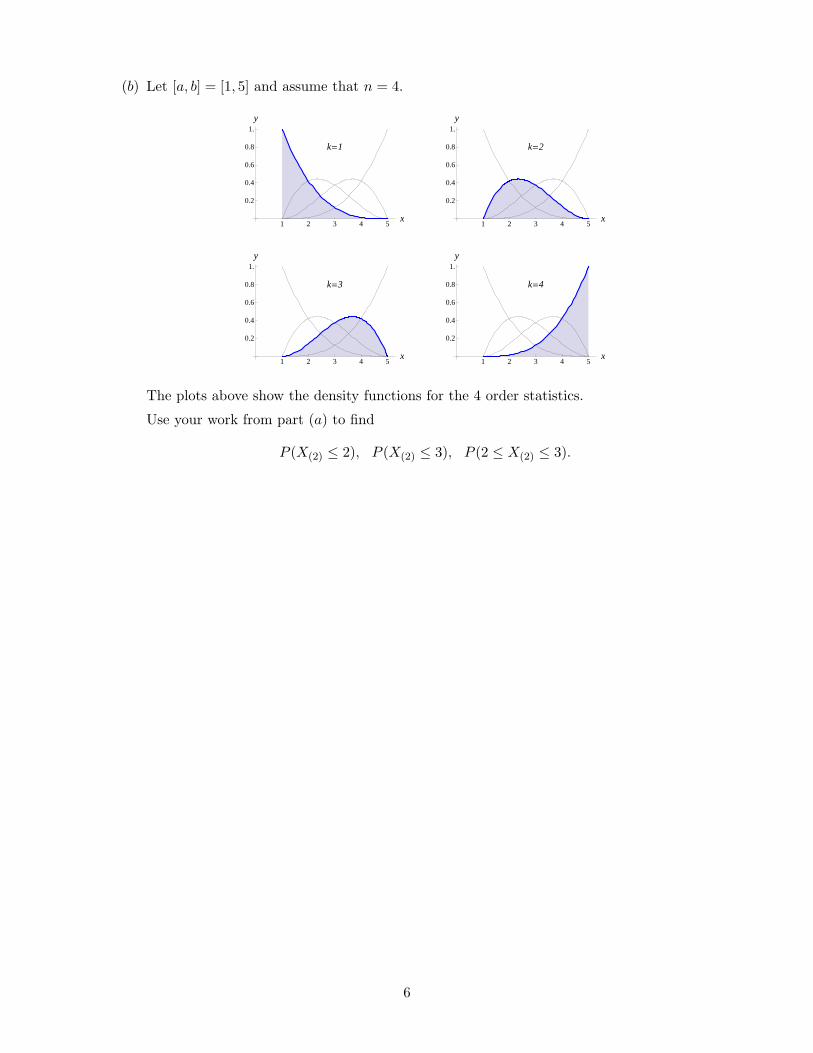
(b) Let [a, b] = [1, 5] and assume that n = 4.

k=1

1 2 3 4 5x

0.2

0.4

0.6

0.8

1.y

k=2

1 2 3 4 5x

0.2

0.4

0.6

0.8

1.y

k=3

1 2 3 4 5x

0.2

0.4

0.6

0.8

1.y

k=4

1 2 3 4 5x

0.2

0.4

0.6

0.8

1.y

The plots above show the density functions for the 4 order statistics.

Use your work from part (a) to find

P (X(2) ≤ 2), P (X(2) ≤ 3), P (2 ≤ X(2) ≤ 3).

6

Exercise. Let X be an exponential random variable with parameter λ.

(a) Let X(k) be the kth order statistic of a random sample of size n from the X distribution.Find simplified expressions for

f(k)(x) and F(k)(x) when x ∈ (0,∞).

7

(b) Let λ = 110 and assume that n = 5.

k=1

10 20 30 40x

0.05

0.15

0.25

y

k=2

10 20 30 40x

0.05

0.15

0.25

y

k=3

10 20 30 40x

0.05

0.15

0.25

y

k=4

10 20 30 40x

0.05

0.15

0.25

y

k=5

10 20 30 40x

0.05

0.15

0.25

y

The plots above show the density functions for the 5 order statistics.

Use your work from part (a) to find

P (X(4) ≤ 10), P (X(4) ≤ 20), P (10 ≤ X(4) ≤ 20).

8

Exercise: Sample Maximum/Minimum. The sample maximum and sample minimum ofa random sample of size n from the X distribution are used in many computations.

(a) Simplify the general formulas for F(n)(x) and f(n)(x) as much as possible.

(b) Simplify the general formulas for F(1)(x) and f(1)(x) as much as possible.

9

Exercise: Quantiles of Sample Maximum/Minimum for uniform distributions.Let X be a uniform random variable on the interval [a, b], and consider the sample maximumand sample minimum of a random sample of size n from the X distribution.

(a) Find a general formula for the pth quantile of the X(n) distribution.

(b) Let [a, b] = [1, 5] and assume n = 4. Use your answer to part (a) to find the median ofthe distribution of the sample maximum.

10

(c) Find a general formula for the pth quantile of the X(1) distribution.

(d) Let [a, b] = [1, 5] and assume n = 4. Use your answer to part (c) to find the median ofthe distribution of the sample minimum.

11

4.1.3 Approximate Mean and Variance of Order Statistic Distributions

Theorem (Summary Measures for K th Order Statistic). LetX be a continuous randomvariable with PDF f(x). In addition, let

1. X(k) be the kth order statistic of a random sample of size n from the X distribution,

2. θ be the pth quantile of the X distribution, where p = kn+1 .

If f(θ) 6= 0, then

E(X(k)) ≈ θ and V ar(X(k)) ≈p(1− p)

(n+ 2)(f(θ))2.

Notes:

1. The theorem tells us that the (n+ 1) intervals

(−∞, E(X(1))), (E(X(1), E(X(2))), . . . , (E(X(n−1), X(n))), (E(X(n)),∞)

. . .EHXH1LL EHXH2LL EHXHnLL

are approximately equally likely. That is,

P (X ∈ The ith Interval) ≈ 1n+ 1

, for i = 1, 2, . . . , n+ 1.

2. The formulas given in the theorem are exact for uniform distributions.

To illustrate the theorem for uniform distributions, let [a, b] = [1, 5] and assume that n = 4.Summary measures for the 4 order statistics are given below:

E(X(k)) V ar(X(k))

k = 1 9/5 32/75

k = 2 13/5 16/25

k = 3 17/5 16/25

k = 4 21/5 32/75

12

4.1.4 Graphical Analysis: Probability Plots

Let X be a continuous random variable, and x(1), x(2), . . . , x(n) be the observed values ofthe order statistics of a random sample of size n from the X distribution.

A probability plot is a plot of pairs of the form:((k

n+ 1

)st

model quantile, x(k)

), k = 1, 2, . . . , n .

The theorem in the last section tells us that the ordered pairs in a probability plot should lieroughly on the line y = x.

For example, I used the computer to generate a random sample of size 95 from the normaldistribution with mean 0 and standard deviation 10.

1. Probability Plot: The plot on the right is a probabil-ity plot of pairs of the form((

k

96

)th

model quantile, x(k)

)

for k = 1, 2, . . . , 95. In the plot, the Observed orderstatistic (vertical axis) is plotted against its approx-imate Expected value (horizontal axis).

-30 -20 -10 0 10 20 30Exp-30

-20

-10

0

10

20

30

Obs

2. Comparison Plot: The plot on the right shows anempirical histogram of the same sample, superim-posed on the density curve for a normal distributionwith mean 0 and standard deviation 10.

Twelve subintervals of equal length were used to con-struct the empirical histogram.

-20 -10 0 10 20 30x0.00

0.01

0.02

0.03

0.04

Density

Footnotes: If n is large, then both plots give good graphical comparisons of model and data.

But, if n is small to moderate, then the probability plot may be a better way to compare modeland data since the shape of the empirical histogram may be very different from the shape ofthe density function of the continuous model.

13

4.2 Estimation and Hypothesis Testing Methods

4.2.1 Large Sample Theory: Sample Median

The following theorem tells us that the sampling distribution of the sample median is approx-imately normal when n is a large, odd integer.

Theorem (Sampling Distribution). Let X be a continuous random variablewith density function f(x), and with median θ. Further, let n be an odd integerand

θ̂ = X(n+12 ) be the sample median of a random sample of size n.

If f(θ) 6= 0 and n is large, then the distribution of

θ̂ is approximately normal with mean θ and variance 14n(f(θ))2

.

4.2.2 Approximate Confidence Interval Procedure for the Median

Under the conditions of the theorem above, an approximate 100(1 − α)% confidence intervalfor the median of the X distribution has the following form:

θ̂ ± z(α/2)

√1

4n(f̂(θ))2where θ̂ = X(n+1

2 ),

and z(α/2) is the 100(1 − α/2)% point of the standard normal distribution. In this formula,f̂(θ) is the estimate of f(θ) obtained by substituting the sample median for θ.

Exercise. Let X be a Cauchy random variable with center θ and spread 1.

The density function of X is

f(x) =1

π(1 + (x− θ)2)

for all real numbers x.

The median of the Cauchy distribution is θ; themean is indeterminate. Θ

fHΘL

(a) Evaluate the variance formula 14n(f(θ))2

.

14

(b) Assume the following data are the values of a random sample of size 75 from the Cauchydistribution with center θ and spread 1.

−88.043 −15.284 −11.278 −1.451 1.830 1.838 2.571 2.987 3.056 3.1883.275 4.145 4.610 4.681 4.705 4.839 4.909 4.922 4.978 5.0485.165 5.193 5.302 5.308 5.380 5.401 5.412 5.443 5.457 5.6365.652 5.792 5.794 5.822 5.826 5.935 5.944 5.985 5.991 6.0596.170 6.185 6.239 6.255 6.301 6.350 6.351 6.411 6.448 6.4496.485 6.515 6.521 6.556 6.571 6.600 6.784 6.846 6.866 6.8696.885 7.215 7.302 7.693 7.776 7.833 7.844 8.455 8.828 9.258

10.984 11.232 11.270 11.365 37.091

-80 -60 -40 -20 0 20x

Use the normal approximation to the distribution of the sample median to construct anapproximate 90% confidence interval for θ.

15

4.2.3 Exact Confidence Interval Procedures for Quantiles

Let X be a continuous random variable, and let θ be the pth quantile of the X distribution,for some proportion p ∈ (0, 1).

Let X(k) be the kth order statistic of a random sample of size n from the X distribution. Then

1. Intervals: The n order statistics divide the real line into (n+ 1) intervals:

(−∞, X(1)), (X(1), X(2)), . . . , (X(n−1), X(n)), (X(n),∞)

(ignoring the endpoints).

2. Binomial Probabilities: The probability that θ lies in a given interval follows a binomialdistribution with parameters n and p. Specifically,

(a) First Interval: The event “θ ∈ (−∞, X(1))” is equivalent to the event that all Xi’sare greater than θ. Thus,

P (θ ∈ (−∞, X(1))) = (1− p)n.

(b) Middle Intervals: The event “θ ∈ (X(k), X(k+1))” is equivalent to the event thatexactly k Xi’s are less than θ. Thus,

P (θ ∈ (X(k), X(k+1))) =(n

k

)pk(1− p)n−k.

(c) Last Interval: The event “θ ∈ (X(n),∞)” is equivalent to the event that all Xi’s areless than θ. Thus,

P (θ ∈ (X(n),∞)) = pn.

Let p(k) =(nk

)pk(1− p)n−k, k = 0, 1, . . . , n, be the binomial probabilities.

Then the following graphic illustrates the probabilities associated with each subinterval.

. . .XH1L XH2L XH3L XHnL

pH0L pH1L pH2L pHnL

Further, the facts above can be used to construct a confidence interval procedure for quantiles.

16

Quantile Confidence Interval Theorem. Under the conditions above, if indicesk1 and k2 are chosen so that

P (θ < X(k1)) =∑k1−1

j=0

(nj

)pj(1− p)n−j = α/2

P (X(k1) < θ < X(k2)) =∑k2−1

j=k1

(nj

)pj(1− p)n−j = 1− α

P (θ > X(k2)) =∑n

j=k2

(nj

)pj(1− p)n−j = α/2

then the interval[X(k1), X(k2)

]is a 100(1− α)% confidence interval for θ.

Note that, in practice, k1 and k2 are chosen to make the sums in the theorem as close aspossible to the values shown on the right.

Exercise (Source: Sheaffer et al, 1996). The following table shows the total yearly rainfall (ininches) for Los Angeles in the 10-year period from the beginning of 1983 to the end of 1992.

1983 1984 1985 1986 1987 1988 1989 1990 1991 1992Rainfall 34.04 8.90 8.92 18.00 9.11 11.57 4.56 6.49 15.07 22.56

Assume these data are the values of a random sample from a continuous distribution.

(a) Construct a 90% (or as close as possible) confidence interval for the median rainfall. Statethe exact confidence level.

p(0) = 0.001x(1) =

p(1) = 0.010x(2) =

p(2) = 0.044x(3) =

p(3) = 0.117x(4) =

p(4) = 0.205x(5) =

p(5) = 0.246x(6) =

p(6) = 0.205x(7) =

p(7) = 0.117x(8) =

p(8) = 0.044x(9) =

p(9) = 0.010x(10) =

p(10) = 0.001

17

(b) Construct a 90% (or as close as possible) confidence interval for the 40th percentile of therainfalls distribution. State the exact confidence level.

p(0) = 0.0060x(1) =

p(1) = 0.0403x(2) =

p(2) = 0.1209x(3) =

p(3) = 0.2150x(4) =

p(4) = 0.2508x(5) =

p(5) = 0.2007x(6) =

p(6) = 0.1115x(7) =

p(7) = 0.0425x(8) =

p(8) = 0.0106x(9) =

p(9) = 0.0016x(10) =

p(10) = 0.0001

4.2.4 Procedures for Endpoint Parameters

Let X be a continuous random variable.

1. Upper Endpoint/Sample Maximum: If the range of X has upper endpoint θ, then thesample maximum can be used in statistical procedures concerning θ.

2. Lower Endpoint/Sample Minimum: If the range of X has lower endpoint θ, then thesample minimum can be used in statistical procedures concerning θ.

18

The following multipart exercise illustrates the use of the sample minimum.

Exercise. Let X be the continuous random variablewith density function

f(x) =110

e−(x−θ10 ) when x > θ, and 0 otherwise.

Note that this X has a shifted exponential distributionwith shift parameter θ and scale parameter λ = 1

10 .Θ

1�10

Let X(1) be the sample minimum of a random sample of size n from the X distribution.

(a) Completely specify the CDF of X(1): F(1)(x) = P (X(1) ≤ x).

(b) Find a general formula for the pth quantile of the X(1) distribution.

19

(c) Let xp and x1−p be the pth and (1− p)th quantiles of the X(1) distribution.

Use the fact that 1− 2p = P (xp ≤ X(1) ≤ x1−p) to fill-in the following blanks:

P(

≤ θ ≤)

= 1− 2p.

(d) Assume the following data are the values of a random sample from the X distribution:

25.8277, 28.5495, 30.1759, 35.8057, 36.6871, 57.257

Use the result of part (c) to construct a 90% confidence interval for θ.

20

(e) Let n = 8. Find the value of c so that the test with decision rule

Reject θ = 15 in favor of θ < 15 when X(1) ≤ c

is a 5% lower tail test of the null hypothesis θ = 15.

(f) Assume the following data are the values of a random sample from the X distribution:

15.2564, 15.9165, 17.9189, 20.2458, 23.221, 25.3941, 27.2703, 29.8149

Would you accept or reject θ = 15 in this case? What is the observed significance level?

21

4.3 Sample Quantiles

4.3.1 Definitions

Let X be a continuous random variable, let θp be the pth quantile of the X distribution, andlet X(k) be the kth order statistic of a random sample of size n , for k = 1, 2, . . . , n.

1. pth Sample Quantile: For p ∈[

1n+1 ,

nn+1

], the pth sample quantile is defined as follows:

(a) if p = kn+1 for some k, then θ̂p = X(k);

(b) if p ∈(

kn+1 ,

k+1n+1

)for some k, then θ̂p = X(k) + ((n+ 1)p− k)

(X(k+1) −X(k)

).

With this definition, the point (θ̂p, p) is on the piecewise linear curve connecting thesuccessive points (

X(1),1

n+ 1

),

(X(2),

2n+ 1

), . . . ,

(X(n),

n

n+ 1

).

2. Sample Quartiles/Median/IQR: The sample quartiles are the estimates of the 25th, 50th,and 75th percentiles:

q1 = θ̂0.25, q2 = θ̂0.50, q3 = θ̂0.75.

The sample median is q2, and the sample interquartile range is the difference q3 − q1.

For example, suppose that the 5 numbers

1.5, 7.5, 9.4, 10.2, 18.0

are observed. Then

• the sample median is x(3) = 9.4,4.5 9.4 14.1

0.25

0.5

0.75

• the sample first and third quartiles are

q1 = x(1) + 0.50(x(2) − x(1)) = 4.5 and q3 = x(4) + 0.50(x(5) − x(4)) = 14.1,

• the sample interquartile range is q3 − q1 = 9.6.

22

Exercise (Source: Rice textbook, Chapter 10). As part of a study on the effects of an infectiousdisease on the lifetimes of guinea pigs, more than 400 animals were infected.

The data below are the lifetimes (in days) of 45 animals given a low exposure to the disease:

33 44 56 59 74 77 93 100 102 105 107 107 108 108 109115 120 122 124 136 139 144 153 159 160 163 163 168 171 172195 202 215 216 222 230 231 240 245 251 253 254 278 458 555

(a) Find the sample quartiles and sample interquartile range.

(b) Find the sample 90th percentile.

23

4.3.2 Graphical Analysis: Box Plots

A box plot is a graphical display of a data set that shows the sample median, the sampleinterquartile range, and the presence of possible outliers (numbers that are far from the center).Box plots were introduced by John Tukey in the 1970’s.

Let q1, q2 and q3 be the sample quartiles. To construct a box plot:

1. Box: A box is drawn from q1 to q3.

2. Bar: A bar is drawn at the sample median, q2.

3. Whiskers: A whisker is drawn from q3 to the largest observation that is less than or equalto q3 + 1.50(q3 − q1). Another whisker is drawn from q1 to the smallest observation thatis greater than or equal to q1 − 1.50(q3 − q1).

4. Outliers: Observations outside the interval

[q1 − 1.50(q3 − q1), q3 + 1.50(q3 − q1)]

are drawn as separate points. These observations are called the outliers.

For example, a box plot of the lifetimes data from the last exercise is shown below:

0 100 200 300 400 500 600

Low

For the lifetimes data, the interval [q1 − 1.50(q3 − q1), q3 + 1.50(q3 − q1)] is

and the outliers are .

24

Exercise. The following data are birthweights (in ounces) for two groups of children:

(1) Children whose mothers visited their doctors five or fewer times during pregnancy:

49 52 82 93 96 101 108 110 114 114 114 116 120 134

(2) Children whose mothers visited their doctors six or more times during pregnancy:

87 93 97 98 106 108 110 113 116 119 119 129 131 153

These data are compared using box plots:

40 60 80 100 120 140 160

5 or Fewer

6 or More

Find the sample quartiles (q1, q2, q3), and the interval [q1 − 1.50(q3 − q1), q3 + 1.50(q3 − q1)]for each data set.

25

Example (Source: Rice textbook, Chapter 10). Consider side-by-side box plots of the followinglifetimes (in days) of guinea pigs given low, medium, and high exposure to an infectious disease:

1. Low Exposure:

33 44 56 59 74 77 93 100 102 105 107 107 108 108 109115 120 122 124 136 139 144 153 159 160 163 163 168 171 172195 202 215 216 222 230 231 240 245 251 253 254 278 458 555

Sample Summaries: n = 45, median = 153, iqr = 112

2. Medium Exposure:

10 45 53 56 56 58 66 67 73 81 81 81 82 83 8891 91 92 92 97 99 99 102 102 103 104 107 109 118 121

128 138 139 144 156 162 178 179 191 198 214 243 249 380 522

Sample Summaries: n = 45, median = 102, iqr = 69

3. High Exposure:

15 22 24 32 33 34 38 38 43 44 54 55 59 60 6060 61 63 65 65 67 68 70 70 76 76 81 83 87 9196 98 99 109 127 129 131 143 146 175 258 263 341 341 376

Sample Summaries: n = 45, median = 70, iqr = 63.5

The graph suggests a strong relationship betweenlevel of exposure and lifetime. Both

• the sample median lifetime and

• the sample IQR

decrease with increasing exposure.

In addition, as exposure increases, the sample dis-tributions become more skewed.

Low Medium High

0

100

200

300

400

500

600

26

Exercise. I used the computer togenerate 15 random samples, each ofsize 100, from the standard normaldistribution. The samples are dis-played as side-by-side box plots.

1 2 3 4 5 6 7 8 9 10 11 12 13 14 15

-3

0

3

Notice that the boxes are all reasonably symmetric and approximately centered at 0. Noticealso that the boxes have few (if any) outliers.

This problem is concerned with the proportion of observations we might expect to be covered bythe box and whiskers, if sampling is done from the standard normal distribution. Specifically,let Z be the standard normal random variable, and

w1 = z0.25 − 1.50 (z0.75 − z0.25) and w2 = z0.75 + 1.50 (z0.75 − z0.25) ,

where zp is the pth quantile of the standard normal distribution.

Find P (w1 ≤ Z ≤ w2).

27