Not-so-minimal Models. Between Isolation and Imagination · Not-so-minimal Models. Between...
24
Not-so-minimal Models. Between Isolation and Imagination Forthcoming in Philosophy of the Social Sciences * Lorenzo Casini † Abstract What can we learn from ‘minimal’ economic models? I argue that learn- ing from such models is not limited to conceptual explorations—which show how something could be the case—but may extend to explanations of real economic phenomena—which show how something is the case. A model may be minimal qua certain world-linking properties, and yet ‘not-so-minimal’ qua learning, provided it is externally valid. This in turn depends on using the right principles for model building, and not necessarily ‘isolating’ principles. My argument is buttressed by a case study from computational economics, namely two ABMs of asset pricing. Can so-called ‘minimal’ economic models teach us something about real eco- nomic systems? If so, what and how? A debate on the epistemic virtues of highly idealised economic models was triggered by (Sugden, 2000). Sugden claimed that idealised models can, if credible, grant conclusions about the real world. More recently, Gr¨ une-Yanoff (2009) has objected that, although learning from such models is possible, it is also very limited. The models can undermine our confidence in the truth of certain necessity or impossibility hypotheses by showing how something could be the case. However, since they are not isomor- phic to their target, do not make use of laws or isolate any real factor—that is, since they are minimal—they cannot prove that something is the case. * I am grateful to Roberto Ganau, Catherine Herfeld, Gianluca Manzo, Alessio Moneta and two anonymous referees for valuable comments on previous versions of this paper. I also wish to thank the audiences of INEM, Rotterdam, 13-15 June 2013, and ENPOSS, Venice, 3-4 September 2013, where this paper was presented. This work was supported by the Alexander von Humboldt Foundation. † Address: Munich Center for Mathematical Philosophy, Ludwig Maximilians Universit¨ at, Ludwigstraße 31, D-80539 M¨ unchen. Email: [email protected] 1
Transcript of Not-so-minimal Models. Between Isolation and Imagination · Not-so-minimal Models. Between...

Not-so-minimal Models.
Between Isolation and Imagination
Forthcoming in Philosophy of the Social Sciences∗
Lorenzo Casini†
Abstract
What can we learn from ‘minimal’ economic models? I argue that learn-
ing from such models is not limited to conceptual explorations—which
show how something could be the case—but may extend to explanations
of real economic phenomena—which show how something is the case.
A model may be minimal qua certain world-linking properties, and yet
‘not-so-minimal’ qua learning, provided it is externally valid. This in
turn depends on using the right principles for model building, and not
necessarily ‘isolating’ principles. My argument is buttressed by a case
study from computational economics, namely two ABMs of asset pricing.
Can so-called ‘minimal’ economic models teach us something about real eco-
nomic systems? If so, what and how? A debate on the epistemic virtues of
highly idealised economic models was triggered by (Sugden, 2000). Sugden
claimed that idealised models can, if credible, grant conclusions about the real
world. More recently, Grune-Yanoff (2009) has objected that, although learning
from such models is possible, it is also very limited. The models can undermine
our confidence in the truth of certain necessity or impossibility hypotheses by
showing how something could be the case. However, since they are not isomor-
phic to their target, do not make use of laws or isolate any real factor—that is,
since they are minimal—they cannot prove that something is the case.
∗I am grateful to Roberto Ganau, Catherine Herfeld, Gianluca Manzo, Alessio Moneta
and two anonymous referees for valuable comments on previous versions of this paper. I also
wish to thank the audiences of INEM, Rotterdam, 13-15 June 2013, and ENPOSS, Venice, 3-4
September 2013, where this paper was presented. This work was supported by the Alexander
von Humboldt Foundation.†Address: Munich Center for Mathematical Philosophy, Ludwig Maximilians Universitat,
Ludwigstraße 31, D-80539 Munchen. Email: [email protected]
1

Here I argue that minimal economic models can support positive conclusions
about their targets, more precisely explanations. Thus, my claim resonates
with, and elaborates on, Sugden’s views. A model may be minimal qua certain
world-linking properties, and yet ‘not-so-minimal’ qua learning, provided it is
externally valid. This in turn depends on using the right principles for model
building, and not necessarily ‘isolating’ principles. My argument is buttressed
by a case study from computational economics, namely two agent-based models
(ABMs) of asset pricing. Many other economic models are minimal in Grune-
Yanoff’s sense. My conclusion generalises to them, too. Thus, I urge, caution
is needed when evaluating their status: although they might all seem to deal
with purely speculative matters, on closer inspection some may offer important
insights into the mechanisms behind real economic phenomena.
I proceed as follows. In §1 I introduce the debate on minimal models. In §2I present the ABMs of asset pricing and claim that they explain important facts
involving the statistical properties of the financial time series of prices. One may
object to my reading along two lines. First, on the assumption that the ABMs
explain, one may question their minimality. Second, granted their minimality,
one may question that they really explain. In §3 and §4 I rebut both objections,
and argue that the ABMs are, in fact, both minimal and explanatory.
1 Minimal models, minimal learning?
Consider a highly idealised economic model such as Schelling’s checkerboard
model (Schelling, 1978, chap. 4). This model is designed to study the unin-
tended emergence of housing segregation patterns out of uncoordinated indi-
vidual actions. The phenomenon is studied on an artificial grid. Each cell in
the grid corresponds to a space which an artificial agent can occupy. Agents,
belonging to two racial groups, are represented by pennies and dimes. They
aim to satisfy just one preference, viz. they want to live in a cell whose neigh-
bourhood comprises at least a certain proportion of their own group. At each
time step, they can either stay where they are, if their preference is satisfied,
or move to a free cell whose neighbourhood satisfies their preference. As a
result of simulating the agent’s moves, segregation obtains across many initial
distributions of agents on the grid and preference strengths.
There are two main positions on the epistemic role of theoretical models
in economics, namely fictionalism and isolationism. In the fictionalist camp,
Sugden (2000, 2009) argues that idealised economic models are like fictions,
or stories: they are believable depending on how the bits of the story fit to-
gether relative to the story’s environment. Yet, their function is not limited to
2

merely conceptual explorations of what could happen, but extends to validating
hypotheses on what actually happens. In the case of Schelling’s model, each
run of the simulation describes what happens in a world parallel to the actual
world (in a city which could be real), thereby providing support to a hypothesis
concerning the real world (real cities).
In a recent paper, Grune-Yanoff (2009) has argued for an opposite conclu-
sion, appealing to broadly isolationist arguments. He notices that there are a
number of world-linking conditions—among which the ‘isolation’ of real causal
factors1 —on which learning from models depends, but that idealised economic
models do not justify whether, or specify how, such conditions are fulfilled. For
instance, in the case of Schelling’s model:
Although calling the symbols and coins neighbours, and their pat-
terns neighbourhoods, and attributing preferences to them, [Schel-
ling] makes no effort to justify these labels by pointing out any re-
semblance to concrete real-world situations, or by citing regularities
about the real world. Of course, some very general features—such
as the distinguishability of tokens and the spatiality of patterns—
resemble features of real-world neighbourhoods. Yet he does not
justify the way in which the model specifies all these features—
neighbours’ preferences, how neighbours are distinguished, the struc-
ture of the neighbourhood, or how discontented neighbours move—
with reference to the real world at all (Grune-Yanoff, 2009, 88-9).
Grune-Yanoff proposes the following negative characterisation of ‘minimal mod-
els’, in terms of their failure to satisfy specific world-linking conditions:2
[Minimal models are] assumed to lack any similarity, isomorphism
or resemblance relation to the world, to be unconstrained by nat-
1For a brief explication of the isolation procedure, see below. For a thorough presentation
of the method of isolation in economics, see (Maki, 1992). Notice, however, the different role
of isolation for Maki and Grune-Yanoff: whereas for Maki isolation (better: the attempt to
isolate) constitutes the nature of representation (cf. Maki, 2005), for Grune-Yanoff, it is the
(success) criterion a model should meet if it is to represent, a criterion that idealised models
fail to meet (see below; also see Grune-Yanoff, 2011b).2Grune-Yanoff’s is not the only understanding of minimal model on offer. In physics, for
example, minimal models are sometimes interpreted as caricatures (Goldenfeld, 1992, 33) that
allow one to reach exact conclusions and thereby explain physical phenomena, for instance
by means of asymptotic reasoning (Batterman, 2002). However, this notion of minimality
and the associated account of learning from minimal models do not apply to contexts, such
as Schelling’s model and the ABMs of asset pricing, where exact (analytic) solutions are not
available and one must resort to simulations.
3
ural laws or structural identity, and not to isolate any real factors
(Grune-Yanoff, 2009, 83).
The question then arises as to whether it is possible to learn something about
the world from them. Grune-Yanoff claims that learning is possible but—contra
Sugden—limited to conceptual explorations. For both Sugden and Grune-
Yanoff, learning depends on the models’ credibility. However, differently from
Sugden, and in line with his own definition of minimal model, Grune-Yanoff
construes the credibility of minimal models as fully dependent on internal co-
herence, and not on world-linking properties such as coherence with one’s knowl-
edge of causal processes. Learning from minimal models obtains because cred-
ibility at the micro level extends to surprising or counterintuitive macro-level
results. Thus, minimal models can tell us how the world could be. However,
they cannot tell us how the world really is. They grant negative conclusions,
by undermining impossibility and necessity hypotheses, for instance Schelling’s
model shows that racism is not necessary to segregation. However, they do not
grant positive conclusions, whether about general facts or about specific events.
So, minimal models only grant minimal learning. Do they?
In the following, I argue that this need not be the case. Minimal models may
grant positive conclusions, in particular explanations. They may be minimal
qua certain world-linking properties, and yet ‘not-so-minimal’ qua learning.
Before moving on, it is important to consider why Grune-Yanoff maintains
that minimal models have limited explanatory power. In short, the relevant
contrast for understanding what prevents (most) models from granting non-
minimal learning about their targets is ‘models vs experiments’ (Grune-Yanoff,
2011b). Experiments ‘isolate’ explanatory factors (e.g., causes) from a ‘base’ of
other factors. Models don’t—whence their epistemic inferiority.
Suppose one wants to use an experiment to test the explanatory role of
some factor in some target system. One will first test the contribution to the
phenomenon made by the factor in experimental conditions. To this end, one
will ensure that the factor is present and operating. Then, assuming that its
modes of interaction with the other factors are known, one will control for
such interactions.3 If the factor makes a difference to the phenomenon, one
will conclude that the factor partially explains the phenomenon. One will then
export the result to the real system based on the material similarity between
the experimental system and the real system. The more robust the difference
across experimental variation in controlled factors, the stronger the conclusion
with respect to the behaviour of the target in non-controlled conditions.
3Alternatively, one may randomise to ensure that lack of knowledge about the other
factors’ interaction with the tested factor does not affect the significance of the experiment.
4
If instead of an experimental system, one can only manipulate a theoretical
model, a positive conclusion will only be granted in very special circumstances,
and will only be as good as the background knowledge used to build the model.
One must start with a faithful model of the target, such that its potentially ex-
planatory components are clearly mapped onto real features of the target and
are distinguishable from the non-explanatory ones (e.g.: idealised factors; fac-
tors that are in the formal model only to guarantee its tractability; etc.). Then,
a successful isolation of the factor’s contribution to the phenomenon will depend
on omitting or idealising away the interactions with the other factors—without
introducing any idealisation in the explanatory factor itself—and then calcu-
lating the (theoretical) effect of the isolated factor. But this procedure cannot
be successfully carried out in the case of minimal models. Minimal models are
not interpreted with respect to their targets, let alone faithful representations
of them. So, they cannot be used to identify explanatory factors, isolate them
from the other factors, and calculate their effects. Minimal models are only
good for conceptual exploration:
the construction process of theoretical models cannot reveal any
actual constraints of the real world, but only discovers the implica-
tions of the model’s assumptions. Hence, modelling does not offer
the same opportunities of learning as experimenting (Grune-Yanoff,
2011b, 12).
For instance, minimal models grant weaker explanations than experiments
(Grune-Yanoff, 2011a). They only grant potential explanations of the form:
some functional capacity would suffice to produce the phenomenon if such-
and-such a mechanism were present. But they grant neither full explanations,
which presuppose that the model tells ‘the whole truth’ about some target
mechanism, nor partial explanations, which presuppose that the model tells
‘nothing but the truth’ about at least some feature of the mechanism common
to both the model and the target.
In the rest of the paper, I take issue with the last claim. I argue that isolation
is not the only means to partial explanation, and I illustrate an alternative
procedure with reference to two ABMs of asset pricing. This, in turn, implies
that minimal models may grant not-so-minimal learning.
5

2 Asset pricing
2.1 The neoclassical model
The motivation for building ABMs of asset pricing lies in a discomfort with
mainstream, ‘neoclassical’ macroeconomics, both with its unrealistic assump-
tions and its inability to account for certain empirical facts.
A fundamental assumption of neoclassical macroeconomics is the so-called
‘rational expectation hypothesis’ (REH): when agents formulate predictions,
they use all available information and do not make systematic forecasting mis-
takes. This hypothesis is usually held in conjunction with the assumption that
agents choose rationally, that is, their preferences among outcomes obey certain
axioms (e.g., completeness, transitivity), and their choices among alternative
courses of action, which aim to bring about those outcomes, maximise expected
utility. Since agents are homogeneous in the above respects, the sum of their
choices (e.g., their demands for some asset) is equivalent to the choice of one
‘representative’ agent.
The REH entails a general hypothesis about market behaviour, viz. ‘the
‘efficient market hypothesis’ (EMH). In financial markets, the price of an asset
(e.g., a stock, a bond) is a ‘rational expectation equilibrium’ (REE). This is
the solution to an agent maximisation problem, namely the price that satis-
fies best the utility of the representative agent. Since the price always reflects
all available information, the current price is the best estimate of the future
price. Prices follow a ‘random walk’. They randomly fluctuate around the as-
sets’ ‘fundamental values’4, so that the distribution of returns, or relative price
changes, is Gaussian: any deviation from the equilibrium is due to an exoge-
nous shock (i.e., a new piece of information on, say, a technological innovation)
that changes the price unpredictably; but this is immediately interpreted as an
arbitrage opportunity and exploited by the agents, so that the price quickly
reverts to its fundamental value.
Neoclassical macroeconomics is, however, unable to account for most of the
so-called ‘stylised facts’ of finance, that is, for special statistical properties of
the time series of prices (Ross (2003, chap. 12), Rickles (2011, §6), LeBaron
(2006, pp. 1191-1192), Samanidou et al. (2007, p. 411)). In agreement with the
neoclassical model, unconditional distributions of returns at high frequencies
(one day or so) are roughly Gaussian, which entails that the direction of re-
turns is generally unpredictable. However, contrary to the neoclassical model,
4The fundamental value is defined as the ‘discounted sum of future earnings’, and calcu-
lated by summing the future income generated by the asset (interests), and discounting it to
the present value to take into account the delay in receipt.
6

unconditional distributions of returns at lower frequencies (one month or less)
are fat-tailed, that is, have too many observations near the mean, too few in
the mid range and too many in the tails to be normally distributed. Among
the alternative distributions that have been proposed to describe fat tails are
power laws, which are scale-invariant.5 Further stylised facts not predicted by
the neoclassical model are volatility clustering and volatility persistence. Large
(respectively, small) price changes tend to follow large (respectively, small) price
changes, instead of being uniformly distributed. Relatedly, asset returns at dif-
ferent times show a dependency (‘long memory’): although the autocorrelation
of returns6 decays quickly to zero, in agreement with the random walk hypoth-
esis, the autocorrelation of squared returns decays more much slowly, which is
evidence of some predictability at longer horizons.
Notice that the stylised facts are general facts about the statistical prop-
erties of the time series of prices. The ABMs of asset pricing are designed to
reproduce such facts—and not particular historical time series—by simulating
the pricing mechanism. Here I present and discuss two such ABMs, viz. (Lux
and Marchesi, 1999, 2000) and (Arthur et al., 1997; LeBaron et al., 1999).
Their novelty with respect to the neoclassical model is that, contrary to the
REH, agents are heterogeneous. Heterogeneity depends on a non-ideal, or more
realistic, kind of rationality, which may be realised in various ways: agents
may differ with respect to their information, computational ability, behavioural
rules, learning strategies, etc. Representing price formation as a result of aggre-
gating the demands of heterogeneous agents is viewed as an improvement over
the representative agent model. As we shall see, heterogeneity is the engine of
a self-reinforcing mechanism which produces the boom-bust pattern observed
in real financial time series. In both models, the stylised facts obtain as a result
of the endogenous pricing mechanism and in the absence of exogenous shocks.
I will now present the two models in more detail.
2.2 A phase-transition model
The first model, presented in (Lux and Marchesi, 1999, 2000), is inspired by
the phenomenon of phase transition in physics. Traders are divided into two
main groups: fundamentalists, who sell (respectively, buy) when the price is
5Power laws are distributions characterised by a cumulative distribution function Pr(X >
x) ∼ ||x||−α. In a log-log plot where ||x|| is the magnitude of some event, for instance a price
fluctuation, and P (x) is the probability of its occurrence, a power law is a straight line. This
indicates that the distribution is scale invariant.6This is the correlation between values of returns at different times, as a function of their
time difference.
7

Figure 1: Volatility clustering (Lux and Marchesi, 1999, 498).
above (respectively, below) the fundamental value, and chartists (or ‘noise
traders’), who buy or sell depending on whether optimism or pessimism pre-
vails. Chartists, in turn, are subdivided into optimists and pessimists. Traders
can switch between different groups, like particles would switch between differ-
ent states. The number of individuals in these groups determines the aggregate
excess demand, which results in changes in actual price, which in turn affect
the agents’ trading strategy. Changes in fundamental value are governed by a
random process. Switching between groups is governed by time-varying proba-
bility functions: the fundamentalist-chartist switch depends on a comparison of
the respective profits (realised profits for the chartists, expected profits for the
fundamentalists); the optimist-pessimist switch depends on an opinion index
(representing the average opinion among chartists) and the price trend.
The system is at equilibrium when the price is on average at its fundamental
value, there is a balanced proportion of optimists and pessimists, and an arbi-
trary proportion of chartists. This steady state is repelling—that is, the system
is unstable—when either certain parameters are larger than some critical value
or when the proportion of chartists exceeds a critical value, in which case the
system suddenly undergoes a tranquil-to-turbulent phase switch.
Simulation of the system in this steady state generates the aforementioned
stylised facts. For instance, the time series of the market price stays close
to the time series of the fundamental value, in agreement with the hypothe-
sis that price variations are unpredictable (figure 1, top). However, random
changes in fundamental value (and the absence of exogenous shocks) (figure
1, bottom) do not result in similarly normally distributed returns, the time se-
8

Figure 2: Scaling of fundamental value changes, compared with that of raw
returns (bottom) and absolute returns (top) (Lux and Marchesi, 1999, 499).
Figure 3: Dependence of return fluctuations (top) on fraction of chartists in
the market (bottom) (Lux and Marchesi, 2000, 689).
9
ries of returns exhibiting a higher-than-normal frequency of extreme events and
volatility clustering (figure 1, middle). In particular, the modellers show that
the stylised facts depend on the endogenous switching mechanism rather than
on the behaviour of the exogenous force, that is, the changes in fundamental
value. They use ‘detrended fluctuation analysis’ to study the scaling properties
of the average fluctuations F (t) of fundamental values, raw and absolute re-
turns as a function of the time interval t, and to calculate the exponents of the
corresponding power laws (figure 2).7 The analysis reveals that the slope of the
power law of changes in fundamental price is similar to the slope of the power
law of raw returns, but smaller than the slope of the power law of absolute
returns. This is a sign of strong persistence in volatility. And since the scal-
ing properties of absolute returns are different from those of fundamental value
changes, the former cannot depend on the latter. The authors also notice that
for a wide range of parameter values the volatility bursts robustly depend on
whether or not the proportion of chartists in the market exceeds a critical value
(figure 3). Hence, they conclude that the volatility bursts are explained by the
switches between groups driven by chartist behaviour (see Lux and Marchesi
(1999, p. 500) and Lux and Marchesi (2000, p. 679)).
2.3 An evolutionary model
The second model, presented, in (Arthur et al., 1997; LeBaron et al., 1999),
is inspired by the phenomenon of natural selection in evolutionary biology.
Each agent in a population is a ‘theory’ of trading rules. Each theory is like a
genotype, made of 100 strategies, or rules. Each rule is like a chromosome, and
consists in a set of predictors, comprising a condition part (a bit string of market
descriptors) and a forecast part (a parameter vector). The condition part of a
predictor is a string of 1’s or 0’s, which can be interpreted as the current price,
respectively, fulfilling a market condition and not fulfilling the condition. Each
bit represents either fundamental information (dividend price ratios) or chartist
information (price moving averages). The forecast part contains parameters of
a linear forecasting model of price and dividend. At the start of the time
period the current dividend is posted and observed by all agents. Each agent
checks which of his predictors are ‘active’, that is, match the current state of
the market. He then forecasts future price and dividend based on the most
accurate of his active predictors and makes the appropriate bid or offer. The
price is calculated by aggregating over the agents’ demands. At the end of the
time period, the new price and dividend are revealed and the accuracies of the
active predictors are updated, based on what should have been predicted in
7For more on this statistical technique, see Kuhlmann (2011, §3.1).
10
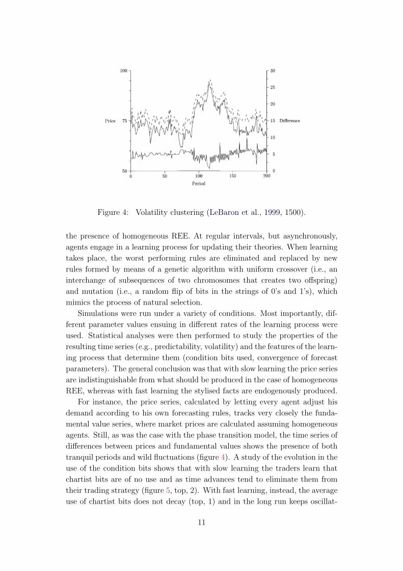
Figure 4: Volatility clustering (LeBaron et al., 1999, 1500).
the presence of homogeneous REE. At regular intervals, but asynchronously,
agents engage in a learning process for updating their theories. When learning
takes place, the worst performing rules are eliminated and replaced by new
rules formed by means of a genetic algorithm with uniform crossover (i.e., an
interchange of subsequences of two chromosomes that creates two offspring)
and mutation (i.e., a random flip of bits in the strings of 0’s and 1’s), which
mimics the process of natural selection.
Simulations were run under a variety of conditions. Most importantly, dif-
ferent parameter values ensuing in different rates of the learning process were
used. Statistical analyses were then performed to study the properties of the
resulting time series (e.g., predictability, volatility) and the features of the learn-
ing process that determine them (condition bits used, convergence of forecast
parameters). The general conclusion was that with slow learning the price series
are indistinguishable from what should be produced in the case of homogeneous
REE, whereas with fast learning the stylised facts are endogenously produced.
For instance, the price series, calculated by letting every agent adjust his
demand according to his own forecasting rules, tracks very closely the funda-
mental value series, where market prices are calculated assuming homogeneous
agents. Still, as was the case with the phase transition model, the time series of
differences between prices and fundamental values shows the presence of both
tranquil periods and wild fluctuations (figure 4). A study of the evolution in the
use of the condition bits shows that with slow learning the traders learn that
chartist bits are of no use and as time advances tend to eliminate them from
their trading strategy (figure 5, top, 2). With fast learning, instead, the average
use of chartist bits does not decay (top, 1) and in the long run keeps oscillat-
11
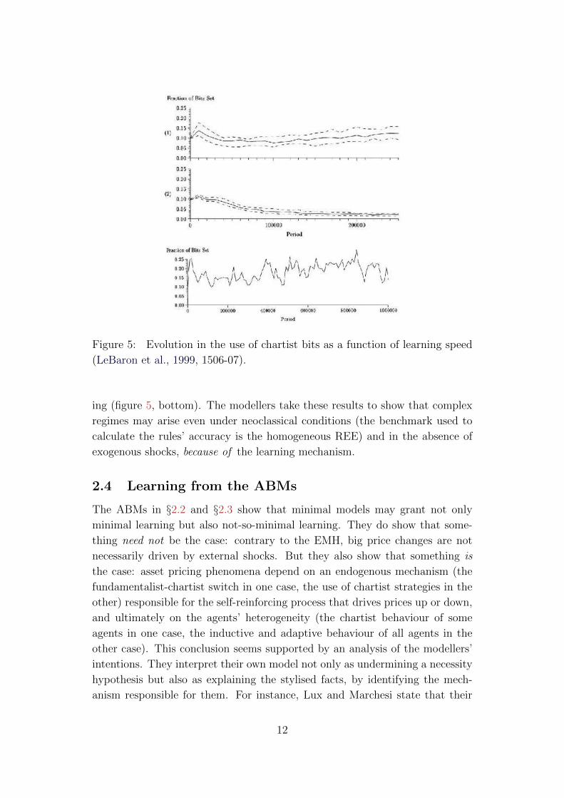
Figure 5: Evolution in the use of chartist bits as a function of learning speed
(LeBaron et al., 1999, 1506-07).
ing (figure 5, bottom). The modellers take these results to show that complex
regimes may arise even under neoclassical conditions (the benchmark used to
calculate the rules’ accuracy is the homogeneous REE) and in the absence of
exogenous shocks, because of the learning mechanism.
2.4 Learning from the ABMs
The ABMs in §2.2 and §2.3 show that minimal models may grant not only
minimal learning but also not-so-minimal learning. They do show that some-
thing need not be the case: contrary to the EMH, big price changes are not
necessarily driven by external shocks. But they also show that something is
the case: asset pricing phenomena depend on an endogenous mechanism (the
fundamentalist-chartist switch in one case, the use of chartist strategies in the
other) responsible for the self-reinforcing process that drives prices up or down,
and ultimately on the agents’ heterogeneity (the chartist behaviour of some
agents in one case, the inductive and adaptive behaviour of all agents in the
other case). This conclusion seems supported by an analysis of the modellers’
intentions. They interpret their own model not only as undermining a necessity
hypothesis but also as explaining the stylised facts, by identifying the mech-
anism responsible for them. For instance, Lux and Marchesi state that their
12

model proves not only that input signals are unnecessary to big price changes,
which contradicts EMH, but also that switching determines the stylised facts:
Financial prices have been found to exhibit some universal charac-
teristics that resemble the scaling laws characterizing physical sys-
tems in which large numbers of units interact. This raises the ques-
tion of whether scaling in finance emerges in a similar way from
the interactions of a large ensemble of market participants. How-
ever, such an explanation is in contradiction to the prevalent ‘ef-
ficient market hypothesis’ in economics, which assumes that the
movements of financial prices are an immediate and unbiased re-
flection of incoming news about future earning prospects. Within
this hypothesis, scaling in price changes would simply reflect similar
scaling in the ‘input’ signals that influence them. Here we describe a
multi-agent model of financial markets which supports the idea that
scaling arises from mutual interactions of participants. Although
the ‘news arrival process’ in our model lacks both power-law scaling
and any temporal dependence in volatility, we find that it generates
such behaviour as a result of interactions between agents (Lux and
Marchesi, 1999, 498, emphases mine).
Arthur et al. express similar remarks. For them, EMH was already suffi-
ciently questioned by previous evidence. Not only does their model confirm this
conclusion, it also uncovers the mechanism responsible for the stylised facts:
By now, enough statistical evidence has accumulated to question
efficient-market theories and to show that the traders’ viewpoint
cannot be entirely dismissed. As a result, the modern finance lit-
erature has been searching for alternative theories that can explain
these market realities (Arthur et al., 1997, §1, emphasis mine)
We conjecture a simple evolutionary explanation. Both in real mar-
kets and in our artificial market, agents are constantly exploring
and testing new expectations. Once in a while, randomly, more
successful expectations will be discovered. Such expectations will
change the market, and trigger further changes in expectations, so
that small and large“avalanches”of change will cascade through the
system (Arthur et al., 1997, §5, emphasis mine)
I anticipate two obvious objections to my reconstruction. First, the ABMs
are not minimal. Second, contrary to the authors’ intentions, they do not
explain. I reply to these objections in, respectively, §3 and §4.
13
3 Minimality defended
Recall the features of minimal models as defined by Grune-Yanoff: minimal
models are not similar, (let alone isomorphic) to the world; they are not built
based on laws; and they do not to isolate any real factors. The ABMs of asset
pricing are prima facie minimal.
First, the ABMs have no strong similarity to their target, nor is there any
clear specification of a concrete target. The models do not aim to approximate,
say, the time series of IBM stocks in some specific time interval. They only
contain fictional individual traders, and ignore the role played by real entities
such as firms, banks, financial and regulatory institutions. Furthermore, the
models misrepresent in clear respects. In the phase transition model, it is
obviously a fiction to represent agents as neatly belonging to either one or the
other category. Also, it is in a sense unrealistic to postulate the existence of
‘unintelligent’ noise traders switching into ‘intelligent’ traders and back, but
being otherwise unable to learn in any other way. Likewise, in the evolutionary
model, it is a fiction to represent the agents’ trading strategies as binary strings
of conditions and a linear forecast. Another unrealistic element is that learning
agents are incapable of adjusting their learning pace by means of a coordination
process. Also unrealistic is that there is no ‘social’ learning between agents,
and all learning goes via the observation of prices. Finally, the learning speed
parameter—on which the stylised facts depend—has no clear interpretation in
terms of real market mechanisms.
Second, the ABMs do not encode laws. There are few, if any, laws in the
social sciences. Some would perhaps take REH as being one such law. The
ABMs, however, do not rely on REH—they actually assume that REH is false.
Or one could interpret the functions that figure in the models as describing
the operation of real capacities or dispositions—the disposition to change one’s
mood, or to learn by trial and error. But whatever the link between such
capacities and their role in the model, the generalisations that describe them
do not certainly count as laws in any strong sense—they are not universal,
necessary, etc.
Finally, the models do not—strictly speaking—isolate any real factors.8
Variables and parameters (groups’ size, switching functions, genotypes, learning
speed, etc.) are hard to interpret—their world-linking properties are unjustified
or undetermined—hence they do not lend themselves to the isolation procedure.
One might think that what is isolated is the agents’ heterogeneity. However, this
is not the case. First, isolation presupposes that interactions with other factors
8On the lack of isolation in idealised economic models, both Sugden and Grune-Yanoff
agree. (See Sugden (2000, §4), Grune-Yanoff (2009, §7) and Grune-Yanoff (2011b).)
14
are omitted or idealised away. But it is at least unclear what factors ‘interact’
with heterogeneity, and how such interactions are controlled for. Secondly, no
idealisation should be introduced in the isolated factor itself, which should be
represented as it is. However, the ABMs’ representation of heterogeneity is the
result of obvious idealisations.
Still, one may object that, contrary to appearances, the ABMs do not count
as minimal models in Grune-Yanoff’s sense, because they do bear some simi-
larity to their targets. As I mentioned, a key feature of minimal models is that
they be credible based on their coherence rather than on similarity considera-
tions. In contrast, the ABMs get at least some credibility from similarity. The
modellers do justify the models’ role as surrogates for something vaguely resem-
bling a real market. For instance, the two artificial markets get some credibility
from analogies. In one case, the market is analogous to a system undergoing
phase transition (cf. Rickles, 2011, §7.3). In the other case, the market is anal-
ogous to a population undergoing natural selection. Also, the artificial markets
are credible because they make (more) plausible psychological assumptions by
giving up the homogeneity assumption. Heterogeneous agents are more similar
to real agents than the homogeneous agents of the neoclassical model.
But then the question is, if the ABMs are not minimal on these grounds,
what models are? Lack of any similarity makes it implausible for a model
to represent anything. And if it were impossible to draw any connection be-
tween the model and the world, it would be a mystery how the model can tell
something—even negatively so—about the world. Some similarity is usually
presupposed for learning from economic models. This seems true even of the
Schelling’s model cited by Grune-Yanoff. Schelling does after all interpret coins
as agents, cells as households, etc. And if a model gets some credibility from
its similarity, is it thereby non-minimal? Arguably, not. I would argue that the
ABMs must be considered minimal after all, in the sense that they approximate
very closely the specific conditions laid out by Grune-Yanoff.
Similarity comes in degrees and in various ways. Grune-Yanoff’s definition
picks out ‘literally minimal’ models, viz. models that bear no similarity to their
targets. Very few, if any, economic models belong to this class—surely nei-
ther the ABMs nor Schelling’s model. At the other end of the spectrum are
models that are similar to their targets in the sense that they are isomorphic
to them, describe laws of nature, isolate natural kind properties, etc. Again,
very few models, whether in economics or in other disciplines, qualify as sim-
ilar in this sense. The majority of scientific models lie somewhere in between
these extremes. Towards the non-minimal end of the spectrum one finds mod-
els that approximate more closely Grune-Yanoff’s conditions. Causal models,
for instance, are typically built out of ceteris paribus generalisations describ-
15

ing dependences among higher-level properties that resemble dependences in
real structures; the generalisations can be studied in isolation and, according
to many, they hold (or fail to hold) depending on more fundamental laws de-
scribing relations among natural kind properties. Towards the minimal end of
the spectrum one finds models such as Schelling’s model and the ABMs of as-
set pricing, which bear weak similarity relations to their targets. Calling them
‘minimal’ seems fully legitimate, in agreement with both philosophical intuition
and scientific practice.9 In the next section, I consider whether and how they
can, in spite of their weak similarity, function as surrogates for their targets
and teach something about them.
4 Explanation defended
As mentioned in §1, Grune-Yanoff holds that (partial) explanation depends on
isolating the effect of some real factors. Clearly, if the ABMs explain at all,
this is not because they isolate something. From this, Grune-Yanoff would
argue that they grant only potential explanations. In contrast, I believe one
should draw a different conclusion: the ABMs show that minimal models may
explain without relying on isolation. It is not the modellers’ intention to offer a
realistic model which allows for the isolation of explanatory factors (see Arthur
et al., 1997, §6). Rather, the aim is to build a model which is credible as a
whole, and not in virtue of the credibility of the individual components. Several
kinds of credibility should be distinguished, which are left undistinguished by
Sugden and Grune-Yanoff, if one is to assess the merits of the corresponding
explanations in their own right.10
On the one hand, ‘credibility-with-respect-to-intuitions’ differs from ‘credi-
bility-with-respect-to-the-target’. As mentioned, Grune-Yanoff proposes that
the credibility of minimal models is analysed in terms of intuitions and coher-
ence considerations. I think this is all well, but it leaves out a part of the story,
namely the issue of assessing the credibility-with-respect-to-the-target, if any,
of minimal models. Economists always construct models as models of some-
9Not only does reference to similarity no useful job in the definition of minimal models, it
is actually misleading. It seems thus sensible to modify the definition by dropping mention
of similarity, viz.: “minimal models are assumed to lack any isomorphism or resemblance
relation to the world, to be unconstrained by natural laws or structural identity, and not to
isolate any real factors”. This allows one to specify the ways in which minimal models are not
similar, but otherwise leave it open that they may be similar in some other, weaker sense.10Maki (2009) offers a somewhat more elaborate classification than I do. The key difference
is that for Maki models have or lack credibility—and thus explanatory force—only insofar as
they isolate or fail to isolate, whereas in my view isolation is not always necessary.
16
thing. It seems undesirable to build into the definition itself of minimal models
that they be credible with respect to intuitions only. This would by fiat prevent
the models from allowing more than merely potential explanations. If one does
not impose this, the possibility remains that one learns from minimal models
because they are credible with respect to their targets, too, and not just intu-
itions. Whether they are credible with respect to their target despite not being
isomorphic to it, not adhering to laws, etc. is a contingent issue—orthogonal
to, and not necessitated by, whether they are minimal.
On the other hand, credibility-with-respect-to-the-target should not be re-
duced to ‘realisticness’, that is, the kind of credibility that depends on isomor-
phisms, adherence to laws, isolation of causal factors, etc. The two kinds of
credibility are different, and grant different kinds of (actual) explanation.11 Re-
alisticness is a stricter condition, which depends on the credibility that individ-
ual components of the model get from isolation (cf. Maki, 1992, §3). Credibility-
with-respect-to-the-target is a weaker condition, which depends on the credi-
bility of the model as a whole. When Sugden talks of credibility being aided
by judgments of coherence with one’s knowledge of causal processes, he seems
to have in mind the latter kind of credibility, not the former. However, the fact
that he does not clearly distinguish between the two weakens his case. One
could, in fact, read him as holding the somewhat inconsistent claim that ide-
alised economic models are credible because they mimic real causal processes,
in the sense that they are isomorphic with them, or isolate them, or represent
causal laws. And I conjecture that Grune-Yanoff’s dichotomous distinction be-
tween minimal and unrealistic models and non-minimal and realistic ones is a
reaction to precisely this latter interpretation of Sugden’s claim.
I think the ABMs case illustrates well the rationale for building credible-
with-respect-to-the-target (minimal) models that are neither realistic, in the
sense of allowing isolation, nor merely credible-with-respect-to-intuitions, in
the sense of allowing conceptual exploration only. I propose that credibility-
with-respect-to-the-target is analysed in terms of the procedures which justify
a model’s external validity. Once one knows whether the model can generate
externally valid results, one also has a justification for believing such results,
that is, for learning from the model.
I draw here on (Winsberg, 1999, 2009)’s account of ‘sanctioning’ a model’s
external validity. For Winsberg, experiments are not intrinsically better than
models. Only, their external validity depends on different kinds of justification
and on—one might say—different kinds of credibility. The external validity
11But I am skeptical that there is any context-independent way of measuring credibility or
explanatory strength.
17

of an experiment depends on realisticness, that is, on some factor in the ex-
perimental system being successfully isolated and on the target system being
materially similar to it in the relevant respect. Instead, the external validity of
a model depends on credibility-with-respect-to-the-target, that is, on making
good use of the right ‘principles for model building’, namely principles that tell
how to build a good model of the target.12 Importantly, good principles are not
necessarily isolating principles, but may vary depending on the model’s target.
In the ABMs case, the following combination of principles make the model
credible-with-respect-to-the-target, and sanction the validity of the explana-
tion: (1) the soundness of theoretical principles, psychological assumptions and
functional analogies; (2) the robustness of the results across changes in ini-
tial conditions and parameter values; and (3) the robustness across changes in
modelling assumptions. Principles in (1) make the model credible-with-respect-
to-the-target, and not just intuitions. Principles in (2) and (3) make the model
credible-with-respect-to-the-target although not realistic.
Let us start with (1). Phenomena such as scaling laws and time series with
complex textures are observed in mechanisms studied by other sciences, too,
from physics (phase transition) to biology (natural selection). There, they are
brought about by dishomogeneities in the constituents of the system (states of
the particles; genetic codes of individuals) that generate self-reinforcing feed-
backs (phase transitions catalysing themselves; genetic traits becoming more
and more entrenched). In spite of the obvious diversity among the various
systems, the explanandum is known to require certain key conditions, viz. het-
erogeneous components and nonlinearities. So, theoretical principles suggest
that these conditions must be instantiated in the asset pricing case, too. The
way the heterogeneity is represented in the market depends on the analogy that
guides the construction of the model: it is as if agents switched or evolved, and
as a result transition- or evolution-cascades obtained. In one case the het-
erogeneity is realised by different dispositions, in the other case by different
expectations. In both cases, the analogy contributes to the credibility of the
model as a whole, because the new psychological assumptions are more plausi-
ble than the neoclassical assumptions. This analogical reasoning is illustrated
by the way Lux and Marchesi motivate their model:
12Winsberg is directly concerned with modelling phenomena for which a background of
sound theories is available. However, his take-home message generalises to other sorts of
background knowledge. Trust in the external validity of the model comes “from a history
of past successes” (Winsberg, 2009, 587); although Winsberg lists three kinds of background
knowledge (theory, intuitive or speculative acquaintance with the system, and reliable com-
putational methods) that warrant such a trust in one case (viz. physics), he leaves it open
that “there may very well be other, similar ones” (ibid.) that are relevant to other cases.
18
(...) an elementary requirement for any adequate analytical ap-
proach is that it must have the potential for bringing about the
required behaviour in theoretical time series. Therefore, it seems
rather obvious that one has to go beyond linear deterministic dy-
namics, which of course is insufficient to account for the phenomena
under study. Furthermore, allowing for homogeneous (white) noise
in some economic variables will also not achieve our goals simply
because (...) we are dealing with time-varying statistical behaviour.
In fact, the situation one faces is more often encountered by natural
scientists. What one wishes to explain is a feature of the empirical
time series as a whole. In the natural sciences, such characteris-
tics of the data are often described by scaling laws (...) (Lux and
Marchesi, 2000, 678).
The modellers include the stylised facts in a broader class of phenomena, and
hypothesise that there is some common feature in the mechanisms that generate
such phenomena. The stylised facts do not depend on the contribution of
linearly independent factors. The isolation of one factor (e.g., the attitude of a
group, or the effect of a trading rule) would eliminate the nonlinear character of
the interactions, hence destroy the self-reinforcing mechanism which generates
the stylised facts. So, credibility is a property of the whole mechanism rather
than isolated portions of it.
The credibility-with-respect-to-the-target is enhanced by the robustness tests
performed on the results, that is, by using principles (2) and (3).
First, the robustness of the results is tested by sensitivity analyses on all
factors for which no clear interpretation or calibration to realistic values is
possible. This involves systematically varying many factors that regulate the
internal working of the mechanism, namely initial conditions (e.g.: initial dis-
tributions of agents in the various groups; initial structure of the trading rules
in the various theories) and parameter values (e.g.: parameters that regulate
the frequency of reevaluation of opinion and the weight exerted on the switch
by the majority’s opinion, the price trend and the profit differential; the pa-
rameter that regulates the learning speed). Since the results are robust across
such variations, one can exclude that they are an artifact of the model design,
that is, that they depend on assumptions that have no representational value
or that involve unrealistic (mis)representations.
Second, the interpretation of the results of the two models shows that the
results are robust in yet another sense—they are robust across variation in mod-
elling assumptions as regards the exact nature of their key explanatory factors,
viz. the agents’ heterogeneity and the self-reinforcing mechanism generated by
19
it. It is as if the modellers employing the aforementioned principles also sub-
scribed to the following meta-principle: the external validity of an explanation
increases if it is possible to show that an entire class of models reproduce the
same phenomenon13, and the mechanisms represented by the models in the
class are different ‘tokens’ of the same ‘type’, each one occupying the same
functional role and carrying some credibility with respect to its target. In the
asset pricing case, the two ABM explanations instantiate the same type of
explanatory pattern, although in different ways. The phase-transition model
explains in terms of different attitudes resulting in a switching feedback, such
that at some times large proportions of chartists are in the market. The evolu-
tionary model explains in terms of different expectations resulting in a learning
feedback, such that at some times certain chartist strategies become useful.
Both models explain by postulating a mechanism where the heterogeneity of
the agents produces an endogenous, self-reinforcing and destabilising feedback.
The rationale for testing the two kinds of robustness (across initial condi-
tions and parameter values, and across different ‘modalities’, or model designs)
to validate the conclusions of simulations is nicely described by Muldoon:
rather than finding the single simulation that uses the appropriate
parameter set to generate the phenomenon, we look for the class of
simulations that generate the phenomenon. One simulation can be
a fluke. A class of simulations that vary by both parameters and
across modalities suggests a robust phenomenon (Muldoon, 2007,
881).
It is instructive to contrast the role of robustness in Schelling’s model and in
the ABMs. The obtaining of the segregation patterns in Schelling’s model is less
robust than the obtaining of the stylised facts in the ABMs. Schelling represents
only one simple type of grid, only two groups of agents, only agents that aim
to satisfy one preference, etc. Schelling does declare that his results will hold
true if other representations are explored (e.g., if square cells are replaced by
triangular cells). But do they? Sugden claims that Schelling’s model grants
knowledge about the world based on an inductive procedure: segregation is
observed in many real cities, and is reproduced by simulating what could happen
in many artificial cities that could be real. However, for this inductive step to
be justified, there seems to be too little variation among the fictional instances.
The result is tested only across different initial distributions of agents on the
same grid and different preference strengths. We have no evidence that, say,
13Ylikoski and Aydinonat (2013) make a similar claim to the point that it is ‘families’ of
theoretical models that provide understanding, and not isolated models.
20

certain housing preferences operate in all cities and are always responsible for
segregation. Different kinds of preferences and other institutional or material
constraints may be at work. Since underlying seemingly similar segregation
patterns there might be very different mechanisms, no one of them can be
invoked without further evidence as ‘the’ explanation of segregation patterns.14
I believe that the lack of robustness across different modelling assumptions may
explain why Grune-Yanoff, who generalises from this exemplary case, holds
that learning from minimal models is limited to undermining necessity and
impossibility hypotheses.
However, things are clearly different in the ABMs case. Each ABM taken
separately allows for a broader exploration of the space of possibilities, because
it controls for many aspects of the postulated mechanisms. And the two ABMs
taken together also offer evidence that the phenomenon is robust across dif-
ferent designs of the mechanism. Thus, learning from the ABMs goes beyond
undermining necessity and impossibility hypotheses. Although we have no ev-
idence that in all markets the stylised facts depend on switching, or that in all
markets they depend on learning, etc., we do have reasonably strong evidence
that in all markets they depend on heterogeneity. So, it seems legitimate to
say that heterogeneity explains the stylised facts.15 16 This explanation has,
to my mind, two key features. First, heterogeneity does not figure as a fac-
tor that may or may not be present but rather as the same factor which can
be variously realised. This makes the explanation general, in the sense that
it does not rely on the truth of any fine-grain hypothesis on the nature of
heterogeneity.17 Secondly, the explanation is partial, in the sense that it only
tells nothing-but-the-truth on one factor responsible for the stylised facts, the
whole truth arguably comprising the role of other factors, such as the exogenous
changes in fundamental value. In general, distinct factors or mechanisms may
positively interact with one another, by amplifying or overdetermining their ef-
fect on the target phenomenon, or they may negatively interact, by decreasing
their effect or pre-empting each other (cf. Ylikoski and Aydinonat, 2013). In
14As Ylikoski and Aydinonat (2013) observe, it is not so much Schelling’s model in and
by itself which provides understanding, but the whole family of models which have been
subsequently built by varying its assumptions.15I am personally inclined to calling this kind of explanation causal. However, arguing for
this claim would require an argument that goes beyond the scope of this paper.16Obviously, one may still want to dispute that this evidence is actually sufficient to expla-
nation. However, this would run contrary not only to my argument (which might be flawed)
but also and more importantly to the scientists’ own interpretation (cf. §2.4), and one would
be left with the task of explaining why their intuition is mistaken.17Among other things, this has the advantage of compensating for the lack of ‘empirical
calibration’ of the models (Fagiolo et al., 2007).
21

the asset pricing case, arguably non-random changes in fundamental value do
not pre-empt the operation of heterogeneity but rather positively interact with
it. At the same time, such changes are not as explanatory of the stylised facts
as heterogeneity: one or more non-random shocks may trigger a bubble or a
crash, but cannot determine the statistical features of volatility as a whole.
One may then wonder whether this sort of explanation is deep enough. As
I said, the two ABMs cannot prove what precise fact about the heterogeneity
of the agents is responsible for the stylised facts. Differences in dispositions
or expectations are not the only ways in which agents may be heterogeneous.
Other models of asset pricing exist, which represent the heterogeneity as depen-
dent on, say, a disagreement on the time required for the price to converge to
the fundamental value, or an asymmetry of knowledge about the fundamental
value, or a difference in the investment horizon for different investors, etc. (cf.
Markose et al., 2007). The variety in the possible realisations of heterogeneity
makes the identified mechanism hard to pin down and put to use. What do the
parameters measure exactly? How can they be used to predict or intervene?
Yet, the generality of the explanation suggests that models leading to more
concrete interpretations, whatever their fine-grain details, will be structurally
similar. For instance, more realistic models (see Schleifer (2000, chap. 4) and
Thurner et al. (2012)), which also represent entities with different roles (private
investors, professional arbitrageurs, funds, banks, etc.) and non-symmetric in-
teractions among them, hold on to the key feature identified by their cognate
minimal models: the stylised facts are explained by some fact or other about
the heterogeneity among the economic agents.
Conclusion
Many economic models are ‘minimal’, in the intuitive sense that they are not
meant to be realistic representations of their targets. Still, they stand in for
such targets. So the question arises: What, if at all, can we learn from them?
In this paper, I have shown that learning from minimal models depends on
the principles for model building that are used in their construction and make
them externally valid. In particular, learning from minimal models need not be
limited to conceptual explorations of what could be the case, and to negative
conclusions, namely to undermining impossibility or necessity hypotheses. If
the right principles are used, minimal models can grant positive conclusions
about what is the case, even if the models are not isomorphic to their targets,
do not make use of laws, and do not isolate real factors. For instance, ABMs of
asset pricing explain the stylised facts of finance in terms of the agents’ hetero-
22

geneity, even if the way the heterogeneity is represented and the mechanisms
the heterogeneity gives rise to are not realistic. The explanation depends on the
identification of a credible pattern through which the heterogeneity generates
the stylised facts via a self-reinforcing feedback mechanism. The credibility of
this pattern is enhanced by the robustness of the results across changes in initial
conditions and parameter values as well as general design principles.
Minimality is orthogonal to external validity: one cannot draw conclusions
about the external validity of a model from the mere fact that it is minimal.
We should not be too quick in generalising from the scarce external validity of
some minimal models (e.g., Schelling’s model) to the lack of external validity
of the others (e.g., ABMs of asset pricing). Rather, we should evaluate them
one by one to find out if they grant just so-stories or something more.
References
Arthur, W. B., LeBaron, B., Palmer, B., and Taylor, R. (1997). Asset Pricing under
Endogenous Expectations in an Artificial Stock Market. In Arthur, W. B., Durlauf,
S. N., and Lane, D. A., editors, Economy as an Evolving Complex System II, vol-
ume XXVII, pages 15–44. Santa Fe Institute Studies in the Science of Complexity,
Reading, MA: Addison-Wesley.
Batterman, R. (2002). Asymptotics and the Role of Minimal Models. British Journal
for the Philosophy of Science, 53:21–38.
Fagiolo, G., Moneta, A., and Windrum, P. (2007). A Critical Guide to Empirical
Validation of Agent-Based Models in Economics: Methodologies, Procedures, and
Open Problems. Computational Economics, 30:195–226.
Goldenfeld, N. (1992). Lectures on Phase Transitions and the Renormalization Group.
Reading, MA: Addison-Wesley.
Grune-Yanoff, T. (2009). Learning from Minimal Economic Models. Erkenntnis,
70(1):81–99.
Grune-Yanoff, T. (2011a). Artificial Worlds and Simulation. In Jarvie, I. C. and
Zamora Bonilla, J., editors, Sage Handbook of Philosophy of Social Science, pages
613–631. London: SAGE Publications.
Grune-Yanoff, T. (2011b). Isolation is not Characteristic of Models. International
Studies in the Philosophy of Science, 25(2):1–19.
Kuhlmann, M. (2011). Mechanisms in Dynamically Complex Systems. In Illari, P.,
Russo, F., and Williamson, J., editors, Causality in the Sciences, pages 880–906.
Oxford University Press.
LeBaron, B. (2006). Agent-based Computational Finance. In Tesfatsion, L. and Judd,
K. L., editors, Handbook of Computational Economics. Agent-based Computational
Economics, volume 2, pages 1187–1233. North Holland: Elsevier.
LeBaron, B. D., Arthur, W. B., and Palmer, R. G. (1999). Time Series Properties of
23
an Artificial Stock Market. Journal of Economic Dynamics and Control, 23:1487–
1516.
Lux, T. and Marchesi, M. (1999). Scaling and Criticality in a Stochastic Multi-agent
Model of a Financial Market. Nature, 397:498–500.
Lux, T. and Marchesi, M. (2000). Volatility Clustering in Financial Markets: A
Microsimulation of Interactive Agents. International Journal of Theoretical and
Applied Finance, 3(4):675–702.
Maki, U. (1992). On the Method of Isolation in Economics. Poznan Studies in the
Philosophy of the Sciences and the Humanities, 26:319–354.
Maki, U. (2005). Models Are Experiments, Experiments Are Models. Journal of
Economic Methodology, 12(2):303–315.
Maki, U. (2009). MISSing the World. Models as Isolations and Credible Surrogate
Systems. Erkenntnis, 70(1):29–43.
Markose, S., Arifovic, J., and Sunder, S. (2007). Advances in Experimental and
Agent-based Modelling: Asset Markets, Economic Network, Computational Mech-
anism Design and Evolutionary Game Dynamics. Journal of Economic Dynamics
and Control, 31:1801–1807.
Muldoon, R. (2007). Robust Simulations. Philosophy of Science, 74(5):873–883.
Rickles, D. (2011). Econophysics and the Complexity of Financial Markets. In Collier,
J. and Hooker, C., editors, Philosophy of Complex Systems, volume 10 of Handbook
of the Philosophy of Science., pages 527–561. North Holland: Elsevier.
Ross, S. M. (2003). An Elementary Introduction to Mathematical Finance. Options
and Other Topics. Cambridge University Press, 2nd edition.
Samanidou, E., Zschischang, E., Stauffer, D., and Lux, T. (2007). Agent-based
Models of Financial Markets. Reports on Progress in Physics, 70:409–450.
Schelling, T. C. (1978). Micromotives and Macrobehaviour. New York: Norton.
Schleifer, A. (2000). Inefficient Markets. An Introduction to Behavioral Finance.
Oxford University Press.
Sugden, R. (2000). Credible Worlds: The Status of Theoretical Models in Economics.
Journal of Economic Methodology, 7(1):1–31.
Sugden, R. (2009). Credible Worlds, Capacities and Mechanisms. Erkenntnis,
70(1):3–27.
Thurner, S., Farmer, J. D., and Geanakoplos, J. (2012). Leverage Causes Fat Tails
and Clustered Volatility. Quantitative Finance, 12(5):695–707.
Winsberg, E. (1999). Sanctioning Models: The Epistemology of Simulation. Science
in Context, 12(2):275–292.
Winsberg, E. (2009). A Tale of Two Methods. Synthese, 169(3):575–592.
Ylikoski, P. and Aydinonat, N. (2013). Understanding with Theoretical Models.
Journal of Economic Methodology, forthcoming.
24