Northwestern European wholesale natural gas prices ...

Int. J. Global Energy Issues, Vol. 42, Nos. 3/4, 2020 259

Copyright © 2020 Inderscience Enterprises Ltd.

Northwestern European wholesale natural gas prices: comparison of several parametric and non-parametric forecasting methods

Hassan Hamie* Energy Economics Group (EEG), Vienna University of Technology, Gusshausstrasse 25-29. A-1040, Vienna, Austria Email: [email protected] *Corresponding author

Anis Hoayek Institute Alexander Grothendieck, University of Montpellier Montpellier, Herault, France Email: [email protected]

Michel Kamel Harvard Extension School, Cambridge, Massachusetts, USA Email: [email protected]

Hans Auer Energy Economics Group (EEG), Vienna University of Technology, Gusshausstrasse 25-29. A-1040, Vienna, Austria Email: [email protected]

Abstract: The ability to understand the stochastic process that governs the changes in natural gas prices is crucial for many reasons. This paper aims to introduce the important methods widely used in econometrics, by linking them to a common ‘use case’ in the subject of commodity pricing. Using the data of natural gas’ weekly prices from 2007 to 2014 of the German gas hub, the methods of least squares, maximum likelihood, machine learning gradient descent, and least squares optimisation are used to compute the coefficients of a multivariate causal regression analysis. This study also tests the short-term prediction of wholesale natural gas prices for each method used. It is found that where the linear approximation is not valid, the method suffers accordingly. However, the mathematical methods of gradient descent and least squares optimisation help visualise the data sets, highlight, and accentuate the nonlinear effects of several variables on the spot gas prices.

260 H. Hamie et al.

Keywords: natural gas; forecasting methods; regression; maximum likelihood; gradient descent; least squares optimisation; machine learning; energy.

Reference to this paper should be made as follows: Hamie, H., Hoayek, A., Kamel, M. and Auer, H. (2020) ‘Northwestern European wholesale natural gas prices: comparison of several parametric and non-parametric forecasting methods’, Int. J. Global Energy Issues, Vol. 42, Nos. 3/4, pp.259–284.

Biographical notes: Hassan Hamie is currently working as a consultant at the Lebanese Petroleum Administration in the Technical and Engineering Department. He received his Masters in Gas Engineering and Management from the École nationale supérieure des mines de Paris and is currently completing his PhD in Energy Economics from the Technische Universität Wien (TU-Wien). The focus of his work is on natural gas modelling through the use of Econometrics.

Anis Hoayek is currently working as associate professor of probability and statistics at the Lebanese University and data scientist at Novelus/B-Yond Company. He received his PhD in probability and statistics from University of Montpellier-France. The focus of his work is on records theory and its applications.

Michel Kamel is currently working as a Senior Director Data Science at B-yond. He holds a master degree in mathematics and actuarial science from the Lebanese University and a Data Science certificate from the Harvard Extension School. He is currently focusing on developing and implementing advanced statistical models for automation and predictive decision making.

Hans Auer is Associate Professor at Energy Economics Group (EEG) at Technische Universität Wien (TU-Wien), Austria. After studying electrical engineering (1996, MSc), he graduated in the field of energy economics (2000, PhD and 2012, Venia Docendi) at TU-Wien. He has been with EEG since 25 years, supplemented by several research stays abroad (e.g. among others, at Lawrence Berkeley National Laboratory (LBNL)/California and Massachusetts Institute of Technology (MIT)/Cambridge). Since the beginning of his academic career, he has dealt with various aspects of energy market design, analyses and modelling both in applied research (coordination of a multitude of European and national projects) as well as teaching and supervision of students at several levels. He also has a significant amount of scientific publications and conference contributions (worldwide).

1 Introduction

The prices of energy commodities are known to have high volatility, and this is a concern to the different stakeholders participating in Energy markets, more specifically policymakers that regulate and dictate the legal framework of these markers. Being able to precisely forecast prices carry direct implications for trading (Efimova and Serletis, 2014).

Unlike oil commodity, the transition of gas into a global market has not yet seen the light. There exist several regional gas markets in today’s world. North America, especially the USA has the most liberalised gas market, where the prices of this commodity vary as a response to its supply and demand.

Northwestern European wholesale natural gas prices 261

This is the result of a solid regulatory reform and widespread investments in infrastructure. Moreover, the US gas market, which consists of several gas hubs, is considered to have a solid integrated structure, where gas prices converge, and this is supportive to the law of one price (Cuddington and Wang, 2006; Holmes et al., 2013).

Several other regional gas markets followed this liberalisation process, which led to the emerging of numerous gas hubs. Traders and shippers located in Europe are transitioning from old legacy long-term contracts to short-term flexible contracts. However, there are still places where the prices of gas do not reflect market supply and demand fundamentals; such is the case of the Asian gas markets. To date, and aside from North America, most of the international gas trade is conducted based on 10- to 30-year long term contracts, with complex price clauses that are indexed to another commodity, which is oil. Supplied volumes and prices, more specifically, the base price (Po) and the index, constitute the most important negotiable items in such a contract (Stern, 2014). In 2010, the European oil-indexed prices played a dominant role, whereas the hub prices played a balancing/arbitrage and subordinate role.

The pressure to liberalise European gas markets has partially broken the link between oil and gas prices. Gas is currently being traded separately on the basis of demand and supply (European Parliament, 2014). In recent years, gas-on-gas competition is becoming more popular and is observed in Europe. The latest data for the total gas priced in Europe for the year 2014 refer to 61% to be hub-based and 32% to be traded under long-term oil-indexed contracts (International Gas Union IGU, 2014).Moreover, in 2011, the European Energy Exchange established a future and a spot market covering the three most important hubs in continental Europe: Net Connect Germany (NCG) and GASPOOL both located in Germany, and the Title Transfer Facility (TTF), located in the Netherlands. Nowadays, market pricing stretches into the rest of Europe through interconnecting pipelines with major hubs (Schultz and Swieringa, 2013).

The spot wholesale gas markets in the UK and the Netherlands offer a second source of gas provisions as opposed to long-term contracts and are thus vital to the overall transactions of gas (ACER, 2011). On the other hand, as pointed out by (Miriello and Polo, 2015), in Germany and Italy a limited and smaller fraction of the total consumed gas is being traded in their hubs that are mostly bought through long-term contracts.

At the moment, Germany is the largest western European gas market. Because of the direct physical connection between the German market areas and the TTF market, there is a strong linkage between both prices. Besides, the NCG market liquidity is higher than that within the other German market GASPOOL, thus, prices should, in theory, respond quickly to changes in supply and demand characteristics.

Several authors study the impact of European integration on the gas market. Neumann and Cullmann (2012) and Petrovich (2016) studied and analysed the prices of eight European gas hubs and measured the level of market integration. Their findings suggest a high level of convergence. Figure 1 illustrates the high price correlation between three different European gas markets (NCG, TTF, and CEGH, the latter representing the Austrian market).

The increased competition on the wholesale market can cause a squeeze in the profit margins of traditional suppliers thus increasing the risk profile. This could lead to greater price volatility.

Using the parametric and non-parametric statistical analysis to study and compute the coefficients of multivariate causal regression analysis, this study aims to contribute and further understand the main drivers of price volatility that affect gas prices on the NCG

262 H. Hamie et al.

gas hub. A short-term prediction of the gas prices for each method will be performed to validate the results.

The remainder of this study is organised as follows: A literature overview is presented in Section 2. The mathematical models and data analyses are explained in Section 3, and in Sections 4 and 5, the results and conclusion will be discussed, respectively.

Figure 1 European wholesale gas prices (€/MWh) (see online version for colours)

2 Literature review and data collection

This section is grouped into four main subjects: the demand and supply features of the gas market, the mathematical models used in recent literature to describe the behaviour of this market, and data collection.

2.1 Demand level

Asche et al. (2008) analysed the elasticity of residential gas demand in 12 European countries. The authors found that the demand is inelastic to the gas prices and income in the short run.

On the other hand, Andersen et al. (2001) focused on industrial gas demand in 11 different industries that are located in 13 different European countries. The authors found that gas demand is price inelastic in the short run. The aforementioned analysis is in line with the fact that the demand of natural gas is inelastic.

Information about the market reaches the market daily; temperature changes tend to cause gas demand variations in the short-term (Mu, 2007). Weather fluctuations influence natural gas prices in north-western Europe, as it is the primary fuel used for heating. Besides, the gas demand in winter in almost every market is higher than that in summer as suggested by Suenaga et al. (2008).

Giulietti et al. (2012) suggested that despite almost the most severe possible test of resilience, demand in the UK gas system was not impacted by the outage of the Rough site, its largest gas storage facility. However, there was, a price to pay, in that gas prices


spiked and demand stayed the same. This shows that gas demand has a much greater sensitivity to temperature than to price.

On the other hand, there are similar price trends for the following three commodities: gas, oil, and coal (European Parliament, 2014). First, there are areas where oil, coal, and gas are substitutes. In the power sector, oil and coal are still the fuel of choice because oil/coal peaking generation units still exist. Thus, a high oil/coal price and/or high CO2 prices would increase the incentive to achieve higher usage of existing gas-fired power-generation capacity, consequently driving up gas demand. Second, most of the big oil companies are active and heavily involved in gas projects. Third and most importantly, Germany imports gas via long-term contracts that are oil price indexed.

The exchange rate between the currency of the importing countries and the United States Dollars (USD) is an important driver for most of the prices of energy commodities. More specifically, the Liquefied Natural Gas (LNG) prices are generally priced in USD. As a result, any change in the dollar value influences the European LNG prices. If the Euro currency depreciates against the USD, it erodes Europe’s ability to compete for available LNG in the global market. The dollar influence also comes through the oil indexation of long-term gas contracts.

2.2 Supply level

Gas supply contracts are either flat or flexible (TimeraEnergy, 2013). The first is relatively price inelastic. The other type of supply is flexible and consequently responds to changes in hub pricing. One of the main supply variables that have a direct effect on gas prices is the storage capacities and how much gas it contains. As noted by (Mu, 2007), storage is crucial in balancing the supply, in markets where the demand fluctuates at all times.

Some storage facilities react to short-term variation in demand, whereas others answer to the seasonal swing. It is reasonable to assume that storage level data will capture the correlation and causality between the prices on the spot market and storage behaviour.

As pointed out by Flouri et al. (2015), from 2006 up to the present, non-European geopolitical and interstate conflicts plaid a major role in disrupting the flow of natural gas and consequently affected the European economy.

LNG terminals also play an important role in the EU’s gas markets. The LNG supplies provide an additional source for gas, in a highly import-dependent region. The EU-28 LNG imports serve as an indicator of supply conditions, and it is believed that they contribute to the spot prices of the NCG hub. Figure 2 summarises the main supply and demand variables that could affect the prices of gas in a certain European gas hub and shows the different potential off-takers of the gas that range from shippers and suppliers to traders and importers and finally the end-users that can be categorised in two different categories: flexible and non-flexible. The difference is that the latter relies more on long-term contracts with a certain amount of take or pay percentage, whereas the other relies on short-term gas contracts mainly bought from the hub.

In opposition to the European market, the US market does not have non-flexible end users. The quick transition of the US market, where all of its gas is being sold and purchased on the basis of gas-to-gas competition, has reformed the structure of contracts. Contracts are now based on hub prices, which explain the popularity of short-term hub contracts.

264 H. Hamie et al.

2.3 Mathematical methods used in literature

A wide literature has been established for volatility modelling. Univariate and multivariate Generalised Autoregressive Conditional Heteroscedasticity (GARCH) methods have been used by Mu (2007) to empirically assess the weather surprises effect on natural gas future, by Ewing et al. (2002) to study the volatility in the markets of oil and gas, and by Efimova and Serletis (2014) to model the volatility of energy markets. Other authors use the Markov regime-switching GARCH methods such as Fong and See (2002) and Jammazi (2014).

Figure 2 European gas market supply and demand and hub prices (see online version for colours)

Hartley et al. (2008), Panagiotidis and Rutledge (2007), Siliverstovs et al. (2005) and Krichene (2002) use the co-integration framework and error correction methods to study the gas markets and some other energy commodities.

Other authors such as Sven-Olaf and Klaus (2010) and Müller et al. (2015) proposed methods that contain deterministic variables such as temperature and oil prices, in addition to a stochastic component. On the other hand, Nick and Thoenes (2014) developed a Vector Autoregressive Analysis (VAR) to study and analyse the effects of several important variables of supply and demand on gas prices. Hamie et al. (2018) applied the theory of the records, which mainly focuses on the study of the tail of the distribution, to compute the probability of a spike or drop in the gas prices.

Other regression modellers use machine learning techniques in the natural gas market. A nonlinear machine learning Neural Network (NN) is used by Busse et al. (2012) to forecast the movement of the gas prices. Moreover, Khotanzad et al. (2000) proposed a two-stage approach to combine several NNs for natural gas consumption. Another use of the gradient descent method can be seen in the work of Salehnia et al. (2013).

Machine learning usage in the gas market is not only limited to gradient descent: Panella et al. (2012) used the NN-maximum likelihood estimation approach, whereas Yilmaz and Kaynar (2011) estimated the coefficients of their regression method using NN-least squares optimisation methods.


2.4 Data collection

Our data set consists of weekly data from September 2007 to December 2014. Table 1 summarises the definition of the variables that will be used in this paper.

Table 1 Data collection

Variable Frequency Description Unit Source

Coal Weekly Coal spot price for Northwestern Europe Euro per ton Global Coal1

heating degree days

Weekly Changes in historical heating degree days (1990–2014)

Degrees Kelvin Degree Days2

Brent oil Weekly Europe Brent Spot Price (dollars per barrel)

Euro per barrelEnergy Information Administration3

Exchange rates Weekly Exchange rate, EUR/USD Unit less Exchange rates4

Storage Weekly Storage utilisation rate for Germany

Percentage points

Gas Infrastructure Europe5

Natural gas, NCG

Weekly Net Connect Germany natural gas spot price

Euro per Megawatt hour

European Energy Exchange6

Research articles contain extensive literature reviews that use Heating Degree Days (HDDs) to assess the weather effect on natural gas spot prices (Sven-Olaf and Klaus, 2010). The non-linear characteristic was observed long ago and used to define the HDD

HDD max 0,k ref kT T (1)

where kT is the average temperature for the k-th week and refT is the reference

temperature, historically set to 288.5 Kelvin .

Deviations from the historical seasonal meteorological pattern are used in this study as determinant of gas prices. This is essential to measure the effect that the unexpected weather has on gas prices.

Spot prices in oil and gas markets are set on a day-ahead basis, whereas in less liquid coal markets, the spot is set on cargos for delivery in the prompt plus 1, 2 and 3 months. We will use the spot prices of Brent for oil prices and the spot prices for the Delivered Ex Ship at Amsterdam (Rotterdam or Antwerp) market, which is the main hub for coal delivered into Europe.

There is not a clear cut between the German spot market and storage behaviour: if there is a lot of seasonal storage booking, a fragment of it can be used for short-term variation. The issue of defining the appropriate market to study price/storage interlink is as follows:

The Western European+ market is more integrated than other markets. Owing this interdependence, more than one country should be assessed while determining the link between price and storage. For example, a lack of supply in country A may be balanced by the supply of country B.

In Eastern Europe, markets are more nationalistic but there is no robust price reference to observe the link between storage and price.

This study will focus on the German storage data only, and it will consider the utilisation rates, to take into account the changes in total storage capacity.

266 H. Hamie et al.

It is not easy to account for possible interrupted supply data, mainly because it cannot be anticipated. Because of the lack of continuous data about LNG delivery, this variable will be omitted from the study.

3 Mathematical methods and data analyses

In this study, the method is referred to as a specific statistical procedure that computes the regression parameters of a certain model to have the best fit regression function. The parameters of each model have to be estimated with an appropriate method of estimation verifying a certain number of assumptions. First, the least squares estimation method is utilised to compute the parameters of the Multi-Linear regression model. On the other hand, the Maxim Likelihood method provides the best quality on bias and standard deviation and is applied to the VAR and Vector Error Correction Model (VECM). Also, the maximum likelihood principle in the context of VAR and VECM converges faster than other estimation procedures.

On the other hand, machine learning techniques are also used in this study, to include non-parametric and nonlinear mathematical methods. These are essentially the gradient descent and the least squares optimisation. Two distinct machine learning models are used and trained to have the best fit: NN and radial basis network.

To characterise the dependent variable, the spot gas prices, some descriptive statistics were performed, and it is clear that the mean and median have similar values. This means that the dependent variable does not include outliers.

The descriptive statistics and the frequency distribution of gas prices shown in Table 2 and Figure 3, lead us to conclude that the dependent variable is close to a normal distribution.

Table 2 Descriptive statistics

Variables N Min Max Mean SD Median

Coal prices 378 57.7 219 98.3 30.1 87.82

Heating degree days 378 266 298 277 6.15 275

Brent prices 378 35.4 142 95.2 21.9 103.1

Exchange rates 378 1.20 1.59 1.36 0.08 1.35

Storage 378 0.17 0.98 0.70 0.21 0.74

Natural gas prices 378 7.37 35.1 21.7 5.45 23.1

SD = standard deviation, N = number of samples

Before analysing the methods, the readers should be reminded of the aim of the study, which is to compute the coefficients of multivariate causal regression analysis and in a second step, to test the short-term prediction of natural gas prices for each method used. For this purpose, the time frame of the study is divided into two parts: September 24, 2007, to January 13, 2014, to compute the regression coefficients and the period of January 20, 2014, to December 15, 2014, to test the efficiency of the methods.

3.1 Least squares method

The first model used in this study is the parametric multiple linear regression; it is used to study the relationship between a dependent variable and one or more independent


variables. It is assumed that each observation in a sample 1 2, , , . . . , , 1 , . . . , i i i iKy x x x i n ,

is generated by an underlying process described by

1 1 2 2 i i i iK K iy x x x (2)

where y is the dependent variable and 1, , kx x are the independent variables.

Figure 3 Frequency distribution of gas prices (see online version for colours)

The term is a random disturbance or a white noise process, it arises primarily because it is not possible to capture every influence on the dependent variable, no matter how elaborated the model is. In this study, the dependent variable is the natural gas spot price, and the independent variables are the supply and demand factors cited in Table 2. How we progress from here depends on the assumption of the stochastic process.

Assumptions of the classical linear regression model are as follows:

1 Linearity: 1 1 2 2 i i i iK K iy x x x . The model specifies a linear relationship

between y and 1 , . . . , .Kx x

2 Full rank: There is no exact linear relationship among any of the independent variables in the model.

3 Exogeneity of the independent variables: 1 2 [ | , , . . . , ] i j j jKE x x x = 0.

4 Homoscedasticity and no-autocorrelation: Each disturbance, i has the same finite

variance, 2 and is uncorrelated with every other disturbance, j . 1 | 0i iE

268 H. Hamie et al.

5 Normal distribution: The disturbances or residuals are normally distributed.

2| ~ 0,X N .

To test for normality and autocorrelation, the Jarque–Bera and the Durbin–Watson tests are used consecutively. The null hypothesis for the model is

0 Independent variable is not useful in explaining the dependent variable , 0iH x Y B

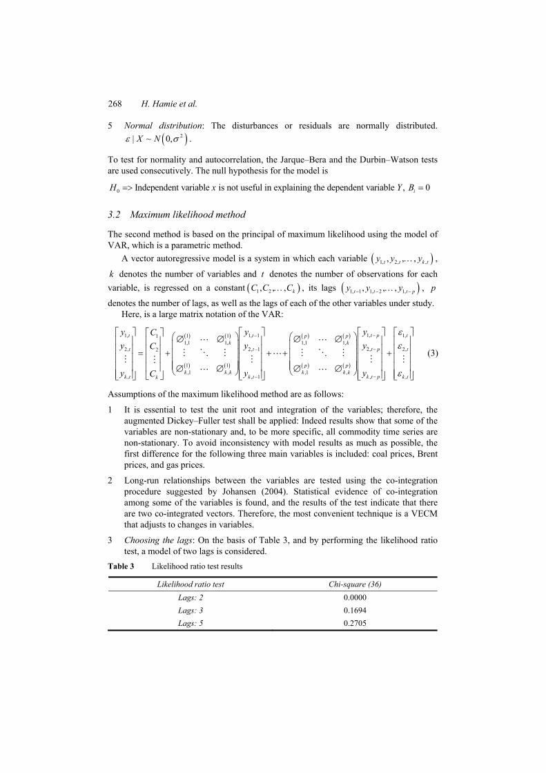
3.2 Maximum likelihood method

The second method is based on the principal of maximum likelihood using the model of VAR, which is a parametric method.

A vector autoregressive model is a system in which each variable 1, 2, ,, , ,t t k ty y y ,

k denotes the number of variables and t denotes the number of observations for each

variable, is regressed on a constant 1 2, , , kC C C , its lags 1, 1 1, 2 1,, , , t t t py y y , p

denotes the number of lags, as well as the lags of each of the other variables under study. Here, is a large matrix notation of the VAR:

1,1, 1, 1 1,1 111,1 1, 1,1 1,

2,2, 2, 1 2,2

1 1,1 , ,1 ,

,, , 1

t pt t tp pk k

t pt t t

p pk k k k k k

k t pk t k tk

yy yC

yy yC

yy yC

,k t

(3)

Assumptions of the maximum likelihood method are as follows:

1 It is essential to test the unit root and integration of the variables; therefore, the augmented Dickey–Fuller test shall be applied: Indeed results show that some of the variables are non-stationary and, to be more specific, all commodity time series are non-stationary. To avoid inconsistency with model results as much as possible, the first difference for the following three main variables is included: coal prices, Brent prices, and gas prices.

2 Long-run relationships between the variables are tested using the co-integration procedure suggested by Johansen (2004). Statistical evidence of co-integration among some of the variables is found, and the results of the test indicate that there are two co-integrated vectors. Therefore, the most convenient technique is a VECM that adjusts to changes in variables.

3 Choosing the lags: On the basis of Table 3, and by performing the likelihood ratio test, a model of two lags is considered.

Table 3 Likelihood ratio test results

Likelihood ratio test Chi-square (36)

Lags: 2 0.0000

Lags: 3 0.1694

Lags: 5 0.2705


As can be seen in Table 3 value of the respective information criteria7 is minimal at the lag count of two.

4 The advantage of the VECM from the linear regression analysis is that it is possible to separate between exogenous and endogenous variables, and this generates an accurate understanding of what drives the gas prices in the short and long term. Table 4 lists the exogenous and endogenous variables. One can argue that harsh weather on a given day can indeed affect the gas prices, yet a change of price will not necessarily affect the weather. Generally, the remaining variables correlate in such a way where the change in one will trigger a change in the other.

Table 4 List of exogenous and endogenous variables

Variables Description Endogenous Exogenous

Coal prices First difference

Heating degree day Heating degree days

Brent prices First difference

Exchange rates Euro–US, exchange rates

Storage Storage utilisation rates

Natural gas prices First difference

It is worth mentioning that, to finalise the choice on which variable to include as exogenous and which one to designate as endogenous, some statistical trial and error work was done on “Gretl” software, by adopting several VECMs combination.

5 To test for normality, the Doornik–Hansen test is used.

3.3 Gradient descent method

3.3.1 Principal component analysis

Before using the gradient descent method, the data will be analysed using a statistical procedure called Principal Component Analysis (PCA). The main objective is to shorten the data set without losing significant information. Several studies have used PCA in multivariate causal analysis, such as Jiang et al. (2015) and Park et al. (2015).

The data are composed of five independent variables, each containing 378 observations, so one can think about a cloud of points in an n-dimensional space R5, and PCA is employed to find and study the relationships among the dataset of 1890 observations. The correlation matrix is shown in Table 5.

Table 5 Correlation matrix

Variables Coal prices

Heating degree days

Brent prices

Exchange rates

Storage Natural gas prices

Coal prices 1 −0.082 0.466 0.597 0.217 0.402

Heating degree days −0.082 1 0.198 −0.218 −0.091 0.249

Brent prices 0.466 0.198 1 0.214 0.094 0.572

Exchange rates 0.597 −0.218 0.214 1 0.136 −0.129

Storage 0.217 −0.091 0.094 0.136 1 0.028

Natural gas prices 0.402 0.249 0.572 −0.129 0.028 1

270 H. Hamie et al.

The PCA results of five supply and demand variables are shown in Table 6 and Figure 4. Four major principle components (F1 to F4) affecting the natural gas prices are identified; combined they explain 93% of the original data variance. The data shown in bold indicate higher loading and contribution to the corresponding components i.e. the high-positive correlation between variable and component. Component, F1, which explains 39% of the total variance, have high loadings on coal, exchange rates, and Brent prices.

Table 6 Rotated factor loadings of principal components on variables

Variables F1 F2 F3 F4

Coal prices 0.635 0.055 0.114 −0.078

Heating degree days −0.117 0.787 −0.148 −0.587

Brent prices 0.438 0.539 0.008 0.632

Exchange rates 0.560 −0.227 0.297 −0.495

Storage 0.278 −0.185 −0.936 −0.068

Figure 4 Bi-plot of the principal components factors (F1 and F2)

-0.5 0 0.5

-0.8

-0.6

-0.4

-0.2

0

0.2

0.4

0.6

0.8

Coal

HDD

Brent

ExchangeStorage

Component 1

Com

pone

nt 2

In the bi-plot shown in Figure 4, vectors represent the adjusted eigenvectors, and the points represent the principal component scores; that is, the representation of space vectors that point in the same direction. This means that the variables have the same response profiles.


The length of the lines approximates the magnitude of the variances of each variable. The cosine of the angle between the lines represents the correlation between the

variables; this means that the smaller the angle, the more the variables are correlated. Since the aim is to reduce the dimension with the variable that has a similar interpretation, consequently, the coal vector was omitted from the study.

Now that the dimension of the data is reduced, the NN gradient descent method can be run. This method is the machine learning nonlinear and non-parametric approach chosen in this study.

3.3.2 Assumptions of the gradient descent method

A neural net consists of a large number of simple processing elements called neurons. Typically, a neuron sends its activation as a signal to several other neurons, with an associated weight

The grouping of neurons into layers and the connection patterns within and between layers is called the net architecture (shown in Figure 5). The most important features of such a network and how it works are well described in the assumptions below.

Figure 5 Back propagation neural network structure illustrative drawing

Assumptions of the gradient descent method:

1 Input vectors contain all the data related to the explanatory variables data used to predict the gas price. Therefore, one input layer contains five neurons.

272 H. Hamie et al.

2 In this study, the two-layer network is used; the first layer, “hidden layer,” contains five neurons, whereas the second layer, “output layer,” is composed of one neuron. The gas price data form the output vector.

3 The authors of this study tried to choose graphically the number of hidden layers; unfortunately, the data are not showing any clusters that are separable by hyper-plane; thus, one hidden layer will be considered.

4 Because there is no significance for the constant and bias in the Multi-Linear Regression, it is assumed that the bias is equal to zero (so both 0v and 0kw are set to

zero).

5 The nets used in the study are feed-forward nets.

6 The gradient descent back propagation is used to train multilayer nets. The back propagation computation is derived using the chain rule of calculus that is found in Hagan et al. (1996).

The next step is to minimise the error term and to do so; the network is trained using the gradient descent back propagation algorithm, so it can learn the underlying relationship between input vectors and the target vector (in other words adjusting the weights). The application divides the data into three sets: training, validation, and testing. In this study, the percentage distribution of data among the three sets is as follows: 70, 15 and 15.

7 Three different nonlinear activation functions are used:

The log-sigmoid function

n

1

1 elogsig n

(4)

The tan-sigmoid function

2

2

1 1ntansig n

e

(5)

The radial basis function (RBF)

2( ) nradbas n e (6)

8 The “hidden layer” 1 _f z in , has three different transfer functions, whereas the

“output layer” has a purelin transfer function g f z . The , ,logsig tansig and

radbas functions are used in artificial NN to introduce non-linearity.

These activation functions have the added benefit of having simple derivatives that make learning the weights of an NN easier. Although theoretically any differentiable function can be used as an activation function, the chosen functions are the most popular nonlinear functions used to explain such type of data in the practical applications.


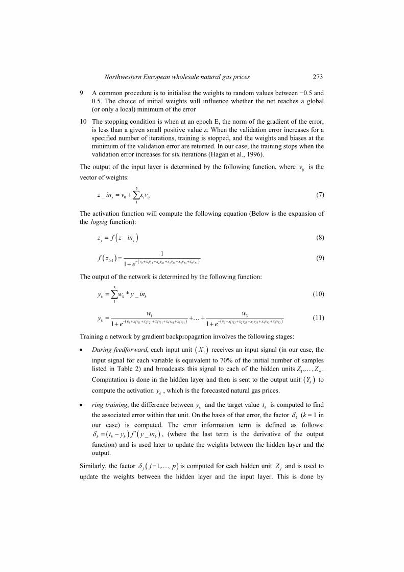
9 A common procedure is to initialise the weights to random values between −0.5 and 0.5. The choice of initial weights will influence whether the net reaches a global (or only a local) minimum of the error

10 The stopping condition is when at an epoch E, the norm of the gradient of the error, is less than a given small positive value . When the validation error increases for a specified number of iterations, training is stopped, and the weights and biases at the minimum of the validation error are returned. In our case, the training stops when the validation error increases for six iterations (Hagan et al., 1996).

The output of the input layer is determined by the following function, where ijv is the

vector of weights:

5

01

_ j i ijz in v x v (7)

The activation function will compute the following equation (Below is the expansion of the logsig function):

_j jz f z in (8)

0 1 11 2 21 3 31 4 41 5 511

1

1in v x v x v x v x v x v

f ze

(9)

The output of the network is determined by the following function:

3

1

* _k k ky w y in (10)

0 1 11 2 21 3 31 4 41 5 51 0 1 13 2 23 3 33 4 43 5 53

1 3

1 1v x v x v x v x v x v v x v x v x v v x vk x

w

e ey

w

(11)

Training a network by gradient backpropagation involves the following stages:

During feedforward, each input unit iX receives an input signal (in our case, the

input signal for each variable is equivalent to 70% of the initial number of samples listed in Table 2) and broadcasts this signal to each of the hidden units 1 , , nZ Z .

Computation is done in the hidden layer and then is sent to the output unit kY to

compute the activation ky , which is the forecasted natural gas prices.

ring training, the difference between ky and the target value kt is computed to find

the associated error within that unit. On the basis of that error, the factor k (k = 1 in

our case) is computed. The error information term is defined as follows:

_k k k kt y f y in , (where the last term is the derivative of the output

function) and is used later to update the weights between the hidden layer and the output.

Similarly, the factor 1 , , j j p is computed for each hidden unit jZ and is used to

update the weights between the hidden layer and the input layer. This is done by

274 H. Hamie et al.

multiplying the derivative of its activation function to calculate its error information

term: _ in _ inj j jf z , where j is the portion of error correction weight

adjustment for ijv .

The weight correction terms are used to update jkw and ijv , and jk k jw z

ij j iv x , where is the learning rate that is used to control the amount of

weight adjustment at each step of training.

And the final step is to update weights and biases; the output unit kY updates

its bias and weights 0, ,j m : new oldjk jk jkw w w , and each

hidden unit , 1 , ,j jZ m updates its bias and weights 0, ,I n :

new oldij ij ijv v v

It is also worth mentioning that each time a feed forward is initialised, the NN parameters are different and consequently generate different solutions due to different initial weight and bias values. As a result, different NNs trained on the same problem can generate different outputs for the same input.

3.4 Least squares optimisation method

The final method of coefficient estimation is the least squares optimisation, and for that purpose, the Radial Basis Network (RBN) will be used. The weights of this network are optimised using the least mean squares algorithm. RBN is based on supervised learning; it can be trained in one stage rather than using the iterative process used in conventional NN. Additionally, RBN is mostly used in models where independent variables affecting the system show nonlinear effects.

Assumptions of the least squares optimisation method are as follows:

1 Input vectors contain all the data related to the explanatory variables data used to predict the gas price.

2 It has the same type of architecture in the sense of perceptron and connections.

3 The output of the input layer is characterised by the following function ;j it is a

non-linear function of unit j, which is typically Gaussian of the form

2

2exp

2jj

XX

(12)

where X and are the input and the centre of RBF unit, respectively. 2 j is the

spread of the Gaussian basis function and is the Euclidian distance between the input vector and the chosen centres of RBF. The centres can be chosen randomly using clustering algorithms.

4 The output layer of the network is derived from this equation:

01

M

k kj j kj

y X W X W

(13)


5 The weights are optimised using the least mean square algorithm. This is done to fit the network outputs to the given inputs.

6 Three different models are used:

The newrb model: It iteratively creates an RBN one neuron at a time, until the sum-squared error reaches zero.

The newr be model: It creates many radbas neurons. In our case, the latter will be the same number as the input vectors.

The grnn model: In this case, the Generalised Regression NN (GRNN) is used for function approximation.

2

2

2

2

2

1

2

1

i

i

Dn

ii

Dn

i

Y eX

e

(14)

The distance, iD , between the training sample and the point of prediction is used as a

measure of how well each training sample can represent the position of prediction, X. For 0iD , the exponential becomes one, and the point of evaluation is represented best

by the training sample.

7 The same spread is used for all the models. Spread is equal to five.

4 Results

4.1 Results for least squares method

It is observed from Table 7 that the p-value for the exchange rates and the storage exceed 5%. Therefore, these variables are not significant and shall be eliminated from the model. Besides, the results show that the model has an R2 of 59.3%, which indicates that the model explains fairly all the variability of the response data around its mean.

Table 7 Least squares results

Variable p-value

Intercept 0.001

Coal prices 7E-11

Heating degree days 2E-16

Brent prices 2E-16

Exchange rates 0.223

Storage 0.012

R2 0.593

Durbin–Watson stat 0.168

Jarque–Bera 9E-06

276 H. Hamie et al.

However, when testing for autocorrelation, the residual plot and the Durbin–Watson test indicate that the residuals are auto-correlated. Besides, the p-value of the Jarque–Beranormality test of residuals exceeds 5%. So the normality assumption is true.

From an economic point of view, the multi linear regression shows that, except for the exchange rates and to lesser extent storage, the other variables chosen in the assumptions have meaningful addition because changes in the value of the variables are related to changes in the gas price.

The higher the R2, the better the linear model fits the data. However, in the first application, the Multi-Linear regression model cannot be considered as the best fit for the simple fact that the assumption of normality and non-autocorrelation of residuals are not valid.

The second method is based on the principal of maximum likelihood applied to the VAR model

4.2 Results for maximum likelihood method

The results show that the gas price is affected mainly by all variables included in the assumptions but for different periods. Also, by considering the VECM, results show that gas prices are directly affected by the lags of all other variables.

Tables 8 and 9 summarise the parameter restrictions on the lagged relationships and the equation of regression for other variables in the VECM. On the basis of these results, it is noted that coal prices depend on the lags of natural gas, coal, and both error correction vectors (having in mind that each error correction vector is a linear combination of several variables that explain the co-integrating relationships); gas prices depend on lags of mainly all other supply and demand variables, although with smaller significance for storage and exchange rates; and so on.

Table 8 Maximum likelihood results

Variable p-value

Intercept 0.0006

Coal prices 0.0015

Heating degree days 0.0670

Brent prices 0.0164

Exchange rates 0.0586

Storage 0.0590

Gas prices 1.33e-05

EC1 4.1e-0.26

EC2 2.3e-0.41

R2 0.518

Durbin–Watson stat 2.017


Table 9 Parameter restrictions on the lagged relationships using the VECM for time (t–1) at a confidence level of 5%

Exchange rates HDD Storage Brent Coal Gas EC1 EC2

HDD

Exchange rates

Storage

Brent

Coal

Gas

At the same time, the results show that gas prices are affected by the following variables: coal prices, exchange rates, and its lags.

The VECM is described with the following mathematical annotation:

1 2 1

3 1 4 1 5 1

6 1 t 1 t 2 1

* *

* * *

* 1 *θ 1 2 *θ 2 *

t t t

t t t

t t

gas constant HDD Storage

Exchange Coal Brent

Gas EC EC dGas

(15)

where denotes the double difference, d designates the first difference, and is the

coefficients computed by the maximum likelihood method of the VECM, which is displayed in Table 8, is the coefficient of the co-integrating vector, and where the error correction vector 1tEC is the co-integrating vector and is its computed

coefficient

1 2 3

4 5 6

* * *

* * * t t t t

t t t

EC constant HDD dStorage dExchange

dCoal dBrent dGas

(16)

Because natural gas is affected by commodity prices and in turn, it also affects the commodity prices and exchange rates, this means that the model captures the economics of energy commodities.

The maximum likelihood-VECM method helps to understand the effects of various fundamental variables on gas prices, and the main conclusion that can be extracted from the method is that, unlike the second assumption in the multi linear regression, there is a clear relationship among the variables of the model.

An additional critical test for the stability of the VECM is the unit root test. The results show that all the inverse roots are contained within the unit circle; this implies that the model is stationary over time.

Both methods used so far require assumptions about the relationship between the independent variables used to produce the gas prices, as well as the probability distribution of residual errors that has to be Gaussian. However, the results show that the VECM normality test failed as the p-value indicates that the normality assumption is rejected; also, at least one of the inverses of roots is almost equal to one. It is expected that the normality test failed because of an outlier in the distribution of residuals, and in the normal case, we can proceed using this model.

278 H. Hamie et al.

4.3 Results for gradient descent method

Figure 6 shows the plots of a forecast of the three models ( , , and logsig Radbas Tansig );

this is the result of the test period composed of 48 values. The predictive power of the gradient descent method and its relevant methods show that the forecasts are acceptable during the test period. The results will be elaborated thoroughly in Sub-section 4.5.

4.4 Results for least squares optimisation method

Figure 7 shows the plot of the function approximation and forecast of the newrb model, which is one of the three models used in the least squares method. As can be seen, the RBN is accurate in approximating the function; however, it does not show the same accuracy during the test period.

Figure 6 Plots of gas forecasts using the neural network gradient descent method

0 5 10 15 20 25 30 35 40 45 5012

14

16

18

20

22

24

26

28

Number of weeks

NC

G p

rices

, E

uro

per M

wh

original function

ApproximationLogsig

ApproximationRadbas

ApproximationTansig

Unlike the two previous forecasting methods that are parametric and constrained by several assumptions on the data, the gradient descent and least squares methods are “constraint-free”. Therefore, there is no need for additional tests (i.e., normality test for residuals and autocorrelation).Also, machine learning forecasting methods perform nonlinear statistical modelling, which helps fitting complex relations in a given data set, and this is asserted in the results shown in Figure 7.

The results of all methods will be compared in Sub-section 4.5.


Figure 7 Plots of spot gas price forecasts using least squares optimisation method (see online version for colours)

4.5 Comparison analyses of all models

So far, eight different models were used to compute the coefficients of a multivariate causal regression analysis. In a final step, the Mean Absolute Percentage Error (MAPE) is solved to validate and compare the models.

1

Target price Forecasted price 1Mean Absolute Percentage Error *100

Target price

ni i

i in

(17)

The results are displayed in Table 10; the mean absolute error is computed twice for each model: one for function approximation and the other for testing and forecasting.

Table 10 Mean absolute percentage error of the different models

Model Coefficient estimation method

Global error for function approximation

(330 weeks)

Global error for testing (forecast–

48 weeks)

Multi linear regression Least squares 15.9 11.45

Vector autoregressive analysis Maximum likelihood

2.22 9.85

logsig Neural Network Gradient descent 7.01 30.69

radbas Neural Network Gradient descent 14.17 15.63

tansig Neural Network Gradient descent 6.71 25.62

280 H. Hamie et al.

Table 10 Mean absolute percentage error of the different models (continued)

Model Coefficient estimation method

Global error for function approximation

(330 weeks)

Global error for testing (forecast–

48 weeks)

newrb Radial Basis Least squares optimisation

5.33 29.25

newrbe Radial Basis Least squares optimisation

0.00 564.4

newgrnn Radial Basis Least squares optimisation

3.95 37.17

It is immature to set arbitrary forecasting targets; to say that a MAPE of <20% is accepted is not a common practice in forecasting, especially when forecasting volatile commodity prices that are governed by different supply and demand fundamentals. However, because the essence of this study is to evaluate and compare the forecasting power of different mathematical methods, the values of MAPE can be used.

As can be seen in Table 10, the highest performance in function approximation is achieved in the maximum likelihood method as well as in the least squares optimisation method. On the other side, most of the models exhibit a MAPE that is ≤ 30%, which, in statistical terms, is a good performance, especially that the analysis is conducted on time series that have more than 300 observations.

Figure 8 depicts the residual error for all models used in this study; i.e., the difference between the predicted values from the models constructed and the observed values are calculated for the period of 6 January 2014 to 15 December 2014.

Target price Forecasted priceResidual error

Target price

(18)

Figure 8 The variation of the values predicted by all models, from the observed values (see online version for colours)

0 5 10 15 20 25 30 35 40 45 50-1.5

-1

-0.5

0

0.5

1

1.5

Number of weeks

Res

idua

l err

or o

f N

CG

pric

es

Radialbasisdesignnew rb

Radialbasisdesignnew rbe

VECM

MLR

MLPradbas

MLPlogsig

MLPtansig

The results are interpreted as follows:

1 The multi linear regression and the VAR imply good estimation with some relaxation of statistical assumption. This would force future modelers to rely on it with caution.


2 Out of the remaining models, both the gradient descent and least squares optimisation, which uses machine learning NN capabilities, succeed in having a low global error.

3 It is also clear that, when it comes to function approximation, the gradient descent NN has a disadvantage over the models used in the least squares optimisation. However, all three models of the former method ( Neural Network logsig ,

Neural Network radbas and the Neural Networktansig ) have consistent results when

used on a new set of data.

4 The least squares optimisation is the technique that performs best in this study. The error results are the lowest for all three models in function approximation. However, one out of three models fails to give valid natural gas price forecasts.

5 Consequently, the models that perform well in approximation use estimation techniques with strong capabilities of memorising but poor performance when generalising on a new set of data.

6 Interestingly, the newrb model has higher capabilities in terms of approximation and with good capabilities while fitting a new set of data, which is crucial in forecasting new short-term gas prices.

5 Conclusions

This paper presents four methods to estimate parameters of regression: least squares, maximum likelihood, machine learning gradient descent, and least squares optimisation. These methods are used to compute the coefficients of multivariate causal regression analysis by linking them to a “use cause” in the subject of commodity pricing, such as natural gas.

The comparison of these methods’ performance shows that there are some clear advantages in using machine learning gradient descent or least squares optimisation over least squares and maximum likelihood. One of the advantages is the matching result of the network’s output and the desired target with low MAPE. Besides, the coefficients computed using the latter method are the most efficient and most accurate when used to forecast short-term natural gas spot day-ahead prices.

However, several supply and demand fundamentals govern the price formula. Rational mathematical and economic interpretations presented in this paper contribute to the understanding of what causes natural gas price volatility in the NCG hub in the first place and succeeds in accurate short-term price forecasts in second place.

The results prove that the non-parametric methods perform best in function approximation, and this is in line with the quality of the data that have a low level of noise. Additionally, the forecasted prices can be trusted as the non-parametric algorithm makes no initial assumption about the data.

The models used in this paper are not only limited to the NCG gas hub but also can be used to forecast natural gas spot prices (both on a daily and weekly bases) in any liberalised natural gas market across Europe. It is worth mentioning that the results of the models described in this paper are data specific; i.e., if additional new variables are used in the same models, this can generate different results. However, the interpretation of the

282 H. Hamie et al.

results will lead to the same conclusion on what causes the volatility in any of the European liberalised natural gas hubs and that the best method to forecast prices based on a multicausal analysis is the NN, more specifically least squares optimisation.

Nevertheless, it is believed that additional mathematical parametric and non-parametric analyses should be done to further analyse and model natural gas prices. Linear models can be employed with the condition of assuming geometric Brownian motion/Radom walk instead of considering only white noise residuals; also, asymmetric GARCH, as well as other nonlinear econometric models, can be employed as an alternative to the “Gaussian” function while trying to model natural gas prices using machine learning methods.

References

ACER (2011) Framework Guidelines on Gas Balancing in Transmission Systems, Ljubljana, Slovenia.

Andersen, T.G., Bollerslev, T., Diebold, F.X. and Ebens, H. (2001) ‘The distribution of realized stock return volatility’, Journal of Financial Economics, Vol. 61, pp.43–76. https://doi.org/10.1016/S0304-405X(01)00055-1

Asche, F., Nilsen, O.B. and Tveterås, R. (2008) ‘Natural gas demand in the European household sector’, Energy Journal, Vol. 29, pp.27–46. https://doi.org/10.5547/ISSN0195-6574-EJ-Vol29-No3-2

Busse, S., Helmholz, P. and Weinmann, M. (2012) ‘Forecasting day ahead spot price movements of natural gas –an analysis of potential influence factors on basis of a NARX neural network’, MultikonferenzWirtschaftsinformatik 2012 – Tagungsband Der MKWI 2012.

Cuddington, J.T. and Wang, Z. (2006) ‘Assessing the degree of spot market integration for U.S. natural gas: evidence from daily price data’, Journal of Regulatory Economics, Vol. 29, pp.195–210. https://doi.org/10.1007/s11149-006-6035-2

Efimova, O. and Serletis, A. (2014) ‘Energy markets volatility modelling using GARCH’, Energy Economics, Vol. 43, pp.264–273. https://doi.org/10.1016/j.eneco.2014.02.018

European Parliament (2014) The impact of the oil price on EU energy prices.

Ewing, B.T., Malik, F. and Ozfidan, O. (2002) ‘Volatility transmission in the oil and natural gas markets’, Energy Economics, Vol. 24, pp.525–538. Doi: 10.1016/S0140-9883(02)00060-9.

Flouri, M., Karakosta, C., Kladouchou, C. and Psarras, J. (2015) ‘How does a natural gas supply interruption affect the EU gas security? A Monte Carlo simulation’, Renewable and Sustainable Energy Reviews. Doi: 10.1016/j.rser.2014.12.029.

Fong, W.M. and See, K.H. (2002) ‘A Markov switching model of the conditional volatility of crude oil futures prices’, Energy Economics, Vol. 24, pp.71–95. Doi: 10.1016/S0140-9883(01)00087-1

Giulietti, M., Grossi, L. and Waterson, M. (2012) ‘A rough analysis: valuing gas storage’, Energy Journal, Vol. 33, pp.119–141. Doi: 10.5547/01956574.33.4.6

Hagan, M., Howard, D., Beale, M. and Jesus, O. (1996) Neural Network Design, 2nd ed., eBook.

Hamie, H., Hoayek, A. and Auer, H. (2018) ‘Modeling the price dynamics of three different gas markets-records theory’, Energy Strategy Reviews, Vol. 21, pp.121–129. Doi: 10.1016/j.esr.2018.05.003

Hartley, P.R., Medlock, K.B. and Rosthal, J.E. (2008) ‘The relationship of natural gas to oil prices’, Energy Journal, Vol. 29, pp.47–65. Doi: 10.5547/ISSN0195-6574-EJ-Vol29-No3-3

Holmes, M.J., Otero, J. and Panagiotidis, T. (2013) ‘On the dynamics of gasoline market integration in the United States: evidence from a pair-wise approach’, Energy Economics, Vol. 36, pp.503–510. Doi: 10.1016/j.eneco.2012.10.008


International Gas Union IGU (2014) Wholesale Gas Price Formation, Fornebu, NORWAY.

Jammazi, R. (2014) ‘Oil shock transmission to stock market returns: wavelet-multivariate markov switching GARCH approach’, Lecture Notes in Energy, Vol. 54, pp.71–111. Doi: 10.1007/978-3-642-55382-0_4

Jiang, Y., Guo, H., Jia, Y., Cao, Y. and Hu, C. (2015) ‘Principal component analysis and hierarchical cluster analyses of arsenic groundwater geochemistry in the Hetao basin’, Inner Mongolia. Chemie der Erde – Geochemistry, Vol. 75, pp.197–205. Doi: 10.1016/j.chemer.2014.12.002

Johansen, S. (2004) Cointegration: An Overview, Working Paper.

Khotanzad, A., Elragal, H. and Lu, T.L. (2000) ‘Combination of artificial neural-network forecasters for prediction of natural gas consumption’, IEEE Transactions on Neural Networks, Vol. 11, pp.464–473. Doi: 10.1109/72.839015

Krichene, N. (2002) ‘World crude oil and natural gas: ademand and supply model’, Energy Economics, Vol. 24, pp.557–576. Doi: 10.1016/S0140-9883(02)00061-0

Miriello, C. and Polo, M. (2015) ‘The development of gas hubs in Europe’, Energy Policy, Vol. 84, pp.177–190. Doi: 10.1016/j.enpol.2015.05.003

Mu, X. (2007) ‘Weather, storage, and natural gas price dynamics: fundamentals and volatility’, Energy Economics, Vol. 29, pp.46–63. Doi: 10.1016/j.eneco.2006.04.003

Neumann, A. and Cullmann, A. (2012) ‘What’s the story with natural gas markets in Europe? Empirical evidence from spot trade data’, Proceedings of the 9th International Conference on the European Energy Market. Doi: 10.1109/EEM.2012.6254679

Nick, S. and Thoenes, S. (2014) ‘What drives natural gas prices? A structural VAR approach’, Energy Economics, Vol. 45, pp.517–527. Doi: 10.1016/j.eneco.2014.08.010

Panagiotidis, T. and Rutledge, E. (2007) ‘Oil and gas markets in the UK: evidence from a cointegrating approach’, Energy Economics, Vol. 29, pp.329–347. Doi: 10.1016/j.eneco.2006.10.013

Panella, M., Barcellona, F. and D’Ecclesia, R.L. (2012) ‘Forecasting energy commodity prices using neural networks’, Advances in Decision Sciences 2012, pp.1–26. Doi: 10.1155/2012/289810

Park, Y.S., Egilmez, G. and Kucukvar, M. (2015) ‘A novel life cycle-based principal component analysis framework for eco-efficiency analysis: case of the United States manufacturing and transportation nexus’, Journal of Cleaner Production, Vol. 92, pp.327–342. Doi: 10.1016/j.jclepro.2014.12.057

Petrovich, B. (2016) Do we have aligned and reliable gas exchange prices in Europe? The oxford institute for Energy Studies, Oxford Institute.

Müller, J., Hirsch, G. and Müller, A. (2015) ‘Modeling the Price of Natural gas with temperature and oil price as Exogenous factors’, Proceedings in Mathematics and Statistics, Springer, pp.109–128. https://doi.org/10.1007/978-3-319-09114-3_7

Salehnia, N., Falahi, M.A., Seifi, A. and MahdaviAdeli, M.H. (2013) ‘Forecasting natural gas spot prices with nonlinear modeling using Gamma test analysis’, Journal of Natural Gas Science and Engineering, Vol. 14, pp.238–249. https://doi.org/10.1016/j.jngse.2013.07.002

Schultz, E. and Swieringa, J. (2013) ‘Price discovery in European natural gas markets’, Energy Policy, Vol. 61, pp.628–634. Doi: 10.1016/j.enpol.2013.06.080

Siliverstovs, B., L’Hégaret, G., Neumann, A. and von Hirschhausen, C. (2005) ‘International market integration for natural gas? A cointegration analysis of prices in Europe, North America and Japan’, Energy Economics, Vol. 27, pp.603–615. Doi: 10.1016/j.eneco.2005.03.002

Stern, J. (2014) ‘International gas pricing in Europe and Asia: acrisis of fundamentals’, Energy Policy, Vol. 64, pp.43–48. Doi: 10.1016/j.enpol.2013.05.127

Suenaga, H., Smith, A. and Williams, J. (2008) ‘Volatility dynamics of Nymex natural gas futures prices’, Journal of Futures Markets, Vol. 28, pp.438–463. Doi: 10.1002/fut.20317

284 H. Hamie et al.

Sven-Olaf, S. and Klaus, W. (2010) ‘A spot price model for natural gas considering temperature as an exogenous factor and applications’, Journal of Energy Markets, Vol. 3, pp.113–128. Doi: 10.21314/JEM.2010.046

TimeraEnergy (2013) A framework for understanding European gas hub pricing [WWW Document]. Available online at: https://timera-energy.com/a-framework-for-understanding-european-gas-hub-pricing/

Yilmaz, I. and Kaynar, O. (2011) ‘Multiple regression, ANN (RBF, MLP) and ANFIS models for prediction of swell potential of clayey soils’, Expert Systems with Applications, Vol. 38, pp.5958–5966. Doi: 10.1016/j.eswa.2010.11.027

Notes

1 Available upon request for research students from the Global Coal Marketing and communication officer, [email protected]

2 Available at http://www.degreedays.net/

3 Available at http://www.eia.gov/dnav/pet/hist/LeafHandler.ashx?n=pet&s=rbrte&f=d

4 Available at http://www.exchange-rates.org/history/EUR/USD/Ton

5 Available at https://transparency.gie.eu/

6 Available upon request for research students from the market and information services, [email protected]

7 Akaike criterion, Schwarz–Bayesian criterion, and Hannan–Quinn criterion

Northwestern European wholesale natural gas prices ...

Documents

Transcript of Northwestern European wholesale natural gas prices ...