NOR THWESTERN UNIVERSITYusers.iems.northwestern.edu/~nocedal/PDFfiles/limited.pdfNOR THWESTERN...

NORTHWESTERN UNIVERSITY

Department of Electrical Engineering

and Computer Science

A LIMITED MEMORY ALGORITHM FOR BOUND

CONSTRAINED OPTIMIZATION

by

Richard H� Byrd�� Peihuang Lu�� Jorge Nocedal� and Ciyou Zhu�

Technical Report NAM��

Revised� May ��

� Computer Science Department� University of Colorado at Boulder� Boulder Colorado �� This author was

supported by NSF grant CCR�� ARO grant DAAL ��G�� and AFOSR grant AFOSR�� Department of Electrical Engineering and Computer Science� Northwestern University� Evanston Il ��

nocedal�eecs�nwu�edu� These authors were supported by National Science Foundation Grants CCR�� and

ASC�� and by Department of Energy Grant DE�FG��ER��A��

�

A LIMITED MEMORY ALGORITHM FOR BOUND

CONSTRAINED OPTIMIZATION

by

Richard H� Byrd� Peihuang Lu� Jorge Nocedal and Ciyou Zhu

ABSTRACT

An algorithm for solving large nonlinear optimization problems with simple bounds is de�

scribed� It is based on the gradient projection method and uses a limited memory BFGS

matrix to approximate the Hessian of the objective function� It is shown how to take advan�

tage of the form of the limited memory approximation to implement the algorithm e�ciently�

The results of numerical tests on a set of large problems are reported�

Key words� bound constrained optimization� limited memory method� nonlinear optimization�quasi�Newton method� large�scale optimization

Abbreviated title� A Limited Memory Method

�� Introduction�

In this paper we describe a limited memory quasi�Newton algorithm for solving large nonlinearoptimization problems with simple bounds on the variables We write this problem as

min fx� ��

subject to l � x � u� ��

where f � �n � � is a nonlinear function whose gradient g is available� the vectors l and urepresent lower and upper bounds on the variables� and the number of variables n is assumedto be large The algorithm does not require second derivatives or knowledge of the structure ofthe objective function� and can therefore be applied when the Hessian matrix is not practical tocompute A limited memory quasi�Newton update is used to approximate the Hessian matrix insuch a way that the storage required is linear in n

�

The algorithm described in this paper is similar to the algorithms proposed by Conn� Gouldand Toint �� and Mor�e and Toraldo �� in that the gradient projection method is used to deter�mine a set of active constraints at each iteration Our algorithm is distinguished from the thesemethods by our use of line searches as opposed to trust regions� but mainly by our use of limitedmemory BFGS matrices to approximate the Hessian of the objective function The propertiesof these limited memory matrices have far reaching consequences in the implementation of themethod� as will be discussed later on We �nd that by making use of the compact representationsof limited memory matrices described by Byrd� Nocedal and Schnabel �� the computational costof one iteration of the algorithm can be kept to be of order n

We used the gradient projection approach �� to determine the active set� becauserecent studies �� indicate that it possess good theoretical properties� and because it alsoappears to be e�cient on many large problems �� However some of the main componentsof our algorithm could be useful in other frameworks� as long as limited memory matrices areused to approximate the Hessian of the objective function

�� Outline of the algorithm�

At the beginning of each iteration� the current iterate xk� the function value fk � the gradientgk� and a positive de�nite limited memory approximation Bk are given This allows us to form aquadratic model of f at xk�

mkx� � fxk� � gTk x� xk� ��

�x� xk�

TBkx� xk��

Just as in the method studied by Conn� Gould and Toint �� the algorithm approximately min�imizes mkx� subject to the bounds given by �� This is done by �rst using the gradientprojection method to �nd a set of active bounds� followed by a minimization of mk treating thosebounds as equality constraints

To do this� we �rst consider the piece�wise linear path

xt� � P xk � tgk� l� u��

obtained by projecting the steepest descent direction onto the feasible region� where

P x� l� u�i �

��

li if xi � lixi if xi � li� ui�ui if xi � ui

��

We then compute the generalized Cauchy point xc� which is de�ned as the �rst local minimizerof the univariate� piece�wise quadratic

qkt� � mkxt��

The variables whose value at xc is at lower or upper bound� comprising the active set Axc�� areheld �xed We then consider the following quadratic problem over the subspace of free variables�

�

min fmkx� � xi � xci � �i � Axc�g ��

subject to li � xi � ui �i �� Axc��

We �rst solve or approximately solve �� ignoring the bounds on the free variables� which canbe accomplished either by direct or iterative methods on the subspace of free variables� or by adual approach� handling the active bounds in �� by Lagrange multipliers When an iterativemethod is employed we use xc as the starting point for this iteration We then truncate the pathtoward the solution so as to satisfy the bounds ��

After an approximate solution �xk�� of this problem has been obtained� we compute the newiterate xk�� by a line search along dk � �xk�� xk that satis�es the su�cient decrease condition

fxk�� fxk� � ��kgTk dk� ��

and that also attempts to enforce the curvature condition

jgTk��dkj � �jgTk dkj� ��

where �k is the steplength and �� are parameters that have the values �� and �� respectively�in our code The line search� which ensures that the iterates remain in the feasible region� isdescribed in x� We then evaluate the gradient at xk�� compute a new limited memory Hessianapproximation Bk�� and begin a new iteration

Because in our algorithm every Hessian approximation Bk is positive de�nite� the approximatesolution �xk�� of the quadratic problem �� de�nes a descent direction dk � �xk�� xk forthe objective function f To see this� �rst note that the generalized Cauchy point xc� which is aminimizer of mkx� on the projected steepest descent direction� satis�es mkxk� � mkx

c� if theprojected gradient is nonzero Since the point �xk�� is on a path from xc to the minimizer of ��along which mk decreases� the value of mk at �xk�� is no larger than its value at xc Therefore wehave

fxk� � mkxk� � mkxc� � mk�xk�� fxk� � gTk dk �

�

�dTkBkdk�

This inequality implies that gTk dk � � if Bk is positive de�nite and dk is not zero In this paperwe do not present any convergence analysis or study the possibility of zigzagging However� giventhe use of gradient projection in the step computation we believe analyses similar to those in ��and �� should be possible� and that zigzagging should only be a problem in the degenerate case

The Hessian approximations Bk used in our algorithm are limited memory BFGS matricesNocedal �� and Byrd� Nocedal and Schnabel �� Even though these matrices do not takeadvantage of the structure of the problem� they require only a small amount of storage and� as wewill show� allow the computation of the generalized Cauchy point and the subspace minimizationto be performed in On� operations The new algorithm therefore has similar computationaldemands as the limited memory algorithm L�BFGS� for unconstrained problems described byLiu and Nocedal �� and Gilbert and Lemar�echal ��

In the next three sections we describe in detail the limited memory matrices� the computationof the Cauchy point� and the minimization of the quadratic problem on a subspace

�

�� Limited Memory BFGS Matrices�

In our algorithm� the limited memory BFGS matrices are represented in the compact formdescribed by Byrd� Nocedal and Schnabel �� At every iterate xk the algorithm stores a smallnumber� say m� of correction pairs fsi� yig� i � k � �� k �m� where

sk � xk�� xk� yk � gk�� gk�

These correction pairs contain information about the curvature of the function� and in conjunctionwith the BFGS formula� de�ne the limited memory iteration matrix Bk The question is how tobest represent these matrices without explicitly forming them

In �� it is proposed to use a compact or outer product� form to de�ne the limited memorymatrix Bk in terms of the n�m correction matrices

Yk � yk�m � � � � � yk�� Sk � sk�m� � � � � sk��

More speci�cally� it is shown in �� that if is a positive scaling parameter� and if the m correctionpairs fsi� yig

k�mi�k�� satisfy s

Ti yi � �� then the matrix obtained by updating I m�times� using the

BFGS formula and the pairs fsi� yigk�mi�k�� can be written as

Bk � I �WkMkWTk ��

whereWk �

hYk Sk

i� ��

Mk �

��Dk LT

k

Lk STk Sk

��

� ��

and where Lk and Dk are the m�m matrices

Lk�i�j �

�sk�m��i�

T yk�m��j� if i � j� otherwise�

��

Dk � diaghsTk�myk�m � � � � � s

Tk��yk��

i� ��

We should point out that �� is a slight rearrangement of equation �� in �� Note thatsince Mk is a �m� �m matrix� and since m is chosen to be a small integer� the cost of computingthe inverse in �� is negligible It is shown in �� that by using the compact representation ��various computations involving Bk become inexpensive In particular� the product of Bk times avector� which occurs often in the algorithm of this paper� can be performed e�ciently

There is a similar representation of the inverse limited memory BFGS matrix Hk that ap�proximates the inverse of the Hessian matrix�

Hk �

I � �Wk

�Mk�WTk � ��

�

where�Wk

h�

�Yk Sk �

i

�Mk

� � �R��

k

�R�Tk R�T

k Dk ��

�Y Tk Yk�R

��

k

��

and

Rk�i�j �

�sk�m��i�

T yk�m��j� if i � j� otherwise

��

We note that �� is a slight rearrangement of equation �� in ��Representations of limited memory matrices analogous to these also exist for other quasi�

Newton update formulae� such as SR� or DFP see �� and in principle could be used for Bk inour algorithm We consider here only BFGS since we have considerable computational experiencein the unconstrained case indicating the limited memory BFGS performs well

Since the bounds on the problem may prevent the line search from satisfying �� see x��we cannot guarantee that the condition sTk yk � � always holds cf Dennis and Schnabel ��Therefore to maintain the positive de�niteness of the limited memory BFGS matrix� we discarda correction pair fsk� ykg if the curvature condition

sTk yk � eps kyk� ��

is not satis�ed for a small positive constant eps If this happens we do not delete the oldestcorrection pair� as is normally done in limited memory updating This means that them directionsin Sk and Yk may actually include some with indices less than k �m

�� The generalized Cauchy point�

The objective of the procedure described in this section is to �nd the �rst local minimizerof the quadratic model along the piece�wise linear path obtained by projecting points along thesteepest descent direction� xk � tgk� onto the feasible region We de�ne x� � xk and� throughoutthis section� drop the index k of the outer iteration� so that g� x and B stand for gk� xk andBk We use subscripts to denote the components of a vector� for example gi denotes the i�thcomponent of g Superscripts will be used to represent iterates during the piece�wise search forthe Cauchy point

To de�ne the breakpoints in each coordinate direction we compute

ti �

��

x�i � ui��gi if gi � �x�i � li��gi if gi � � otherwise�

��

�

and sort fti� i � �� ng in increasing order to obtain the ordered set ftj � tj � tj�� j � �� ngThis is done by means of a heapsort algorithm �� We then search along P x�� tg� l� u�� a piece�wise linear path which can be expressed as

xit� �

�x�i � tgi if t � tix�i � tigi otherwise

Suppose that we are examining the interval tj�� tj � Let us de�ne the j � ��th breakpoint as

xj�� xtj��

so that on tj�� tj �xt� � xj�� tdj��

where�t � t � tj��

and

dj��i �

��gi if tj�� ti� otherwise�

��

Using this notation we write the quadratic �� on the line segment xtj�� xtj�� as

mx� � f � gT x� x��

�x� x��TBx � x��

� f � gT zj�� tdj��

�zj�� tdj��TBzj�� tdj��

wherezj�� xj�� x��

Therefore on the line segment xtj�� xtj�� mx� can be written as a quadratic in �t�

�m�t� � f � gTzj��

�zj��

TBzj�� gTdj�� dj��

TBzj��t

��

�dj��

TBdj��t�

fj�� f �j��t ��

�f ��j��t

��

where the parameters of this one�dimensional quadratic are

fj�� f � gTzj��

�zj��

TBzj��

f �j�� gTdj�� dj��TBzj��

f ��j�� dj��TBdj��

Di�erentiating �m�t� and equating to zero� we obtain �t� � �f �j��f��

j�� Since B is positive

de�nite� this de�nes a minimizer provided tj�� t� lies on tj�� tj� Otherwise the generalizedCauchy point lies at xtj�� if f �j�� and beyond or at xtj� if f �j��

�

If the generalized Cauchy point has not been found after exploring the interval tj�� tj �� weset

xj � xj�� tj��dj�� tj�� tj � tj��

and update the directional derivatives f �j and f ��j as the search moves to the next interval Let us

assume for the moment that only one variable becomes active at tj � and let us denote its indexby b Then tb � tj � and we zero out the corresponding component of the search direction�

dj � dj�� gbeb� ��

where eb is the b�th unit vector From the de�nitions �� and �� we have

zj � zj�� tj��dj��

Therefore using �� and �� we obtain

f �j � gTdj � djTBzj

� gTdj�� g�b � dj��TBzj�� tj��dj��

TBdj�� gbe

Tb Bz

j

� f �j�� tj��f ��j�� g�b � gbeTb Bz

j ��

and

f ��j � djTBdj

� dj��TBdj�� gbe

Tb Bd

j�� g�bebTBeb

� f ��j�� gbeTb Bd

j�� g�bebTBeb� ��

The only expensive computations in �� and �� are

ebTBzj � eb

TBdj�� ebTBeb�

which can require On� operations since B is a dense limited memory matrix Therefore it wouldappear that the the computation of the generalized Cauchy point could require On�� operations�since in the worst case n segments of the piece�wise linear path can be examined This cost wouldbe prohibitive for large problems However� using the limited memory BFGS formula �� andthe de�nition �� the updating formulae �� become

f �j � f �j�� tj��f ��j�� g�b � gbzjb � gbw

Tb MWT zj � ��

f ��j � f ��j�� g�b � �gbwTb MWTdj�� g�b � g�bw

Tb Mwb� ��

where wTb stands for the b�th row of the matrix W The only On� operations remaining in ��

and �� are WTzj and WTdj�� We note� however� from �� and �� that zj and dj areupdated at every iteration by a simple computation Therefore if we maintain the two �m�vectors

pj WTdj �WT dj�� gbeb� � pj�� gbwb�

�

cj WT zj � WT zj�� tj��dj�� cj�� tj��pj��

then updating f �j and f ��j using the expressions

f �j � f �j�� tj��f ��j�� g�b � gbzjb � gbw

Tb Mcj �

f ��j � f ��j�� g�b � �gbwTb Mpj�� g�bw

Tb Mwb�

will require only Om�� operations If more than one variable becomes active at tj � an atypicalsituation � we repeat the updating process just described� before examining the new interval tj � tj�� We have thus been able to achieve a signi�cant reduction in the cost of computing thegeneralized Cauchy point

Remark� The examination of the �rst segment of the projected steepest descent path� during the

computation of the generalized Cauchy point� requires On� operations� However all subsequent

segments require only Om�� operations� where m is the number of correction vectors stored in

the limited memory matrix�

Since m is usually small� say less than �� the cost of examining all segments after the �rstone is negligible The following algorithm describes in more detail how to achieve these savingsin computation Note that it is not necessary to keep track of the n�vector zj since only thecomponent zjb corresponding to the bound that has become active is needed to update fj

� andfj��

Algorithm CP� Computation of the generalized Cauchy point�

Given x� l� u� g� and B � I �WMWT

� Initialize

For i � �� n compute

ti ��

��

xi � ui��gi if gi � �xi � li��gi if gi � � otherwise

n operations�

di ��

�� if ti � ��gi otherwise

F �� fi � ti � � gp �� WTd �mn operations �c �� f � �� gTd � �dTd n operations�f �� dTd� dTWMWT d � �f � � pTMp Om�� operations�

�tmin �� f �

f ��

told �� t �� minfti � i � Fg using the heapsort algorithm�b �� i such that ti � t remove b from F�

�t �� t � �

�

� Examination of subsequent segmentsWhile �tmin � �t do

xcpb ��

�ub if db � �lb if db � �

zb �� xcpb � xb

c �� c��tp Om� operations�

f � �� f � ��tf �� g�b � gbzb � gbwTb Mc Om�� operations�

f �� f �� g�b � �gbwTb Mp� g�bw

Tb Mwb Om�� operations�

p �� p� gbwb Om� operations�

db ��

�tmin �� f �

f ��

told �� t

t �� minfti � i � Fg using the heapsort algorithm�

b �� i such that ti � t Remove b from F�

�t �� t� told

end while

� �tmin �� maxf�tmin� �g

� told �� told � �tmin

� xcpi �� xi � tolddi� � i such that ti � t

� For all i � F with ti � t� remove i from F

� c �� c� �tminp

The last step of this algorithm updates the �m�vector c so that upon termination

c � WT xc � xk��

This vector will be used to initialize the subspace minimization when the primal direct methodor the conjugate gradient method are used� as will be discussed in the next section

Our operation counts only take into account multiplications and divisions Note that thereare no On� computations inside the loop If nint denotes the total number of segments explored�then the total cost of Algorithm CP is �m��n�Om��nint operations plus n logn operationswhich is the approximate cost of the heapsort algorithm ��

�� Methods for subspace minimization�

Once the Cauchy point xc has been found� we proceed to approximately minimize the quadraticmodel mk over the space of free variables� and impose the bounds on the problem We consider

�

three approaches to minimize the model� a direct primal method based on the Sherman�Morrison�Woodbury formula� a primal iterative method using the conjugate gradient method� and a directdual method using Lagrange multipiers Which of these is most appropriate seems problem de�pendent� and we have experimented numerically with all three In all these approaches we �rstwork on minimizing mk ignoring the bounds� and at an appropriate point truncate the move soas to satisfy the bound constraints

The following notation will be used throughout this section The integer t denotes the numberof free variables at the Cauchy point xc� in other words there are n� t variables at bound at xcAs in the previous section F denotes the set of indices corresponding to the free variables� andwe note that this set is de�ned upon completion of the Cauchy point computation We de�neZk to be the n � t matrix whose columns are unit vectors ie columns of the identity matrix�that span the subspace of the free variables at xc Similarly Ak denotes the n� n� t� matrix ofactive constraint gradients at xc� which consists of n � t unit vectors Note that AT

kZk � � andthat

AkATk � ZkZ

Tk � I� ��

�� A Direct Primal Method�

In a primal approach� we �x the n� t variables at bound at the generalized Cauchy point xc�and solve the quadratic problem �� over the subspace of the remaining t free variables� startingfrom xc and imposing the free variable bounds �� Thus we consider only the points x � �n ofthe form

x � xc � Zk�d� ��

where �d is a vector of dimension t Using this notation� for points of the form �� we can writethe quadratic �� as

mkx� � fk � gTk x� xc � xc � xk� ��

�x� xc � xc � xk�

TBkx� xc � xc � xk�

� gk � Bkxc � xk��

T x� xc� ��

�x� xc�TBkx� xc� �

�dT �rc ��

��dT �Bk

�d� � ��

where is a constant��Bk � ZT

k BkZk

is the reduced Hessian of mk� and

�rc � ZTk gk �Bkx

c � xk��

is the reduced gradient of mk at xc Using �� and �� we can express this reduced gradientas

�rc � ZTk gk � xc � xk��WkMkc��

��

which� given that the vector c was saved from the Cauchy point computation� costs �m� ��t�Om�� extra operations Then the subspace problem �� can be formulated as

min �mk �d� �dT �rc � �

��dT �Bk

�d� ��

subject to li � xci ��di � ui � xci i � F � ��

where the subscript i denotes the i�th component of a vector The minimization �� can besolved either by a direct method� as we discuss here� or by an iterative method as discussed inthe next subsection� and the constraints �� can be imposed by backtracking

Since the reduced limited memory matrix �Bk is a small�rank correction of a diagonal matrix�we can formally compute its inverse by means of the Sherman�Morrison�Woodbury formula� andobtain the unconstrained solution of the subspace problem ��

�du � � �B��

k �rc� ��

We can then backtrack towards the feasible region� if necessary� to obtain

�d� � �� du�

where the positive scalar �� is de�ned by

�� maxf� � � � �� li � xci � � �dui � ui � xci � i � Fg� ��

Therefore the approximate solution �x of the subproblem �� is given by

�xi �

�xci if i �� F

xci � Zk�d��i if i � F

��

It only remains to consider how to perform the computation in �� Since Bk is given by�� and ZT

k Zk � I � the reduced matrix �B is given by

�B � I � ZTW �MWTZ��

where we have dropped the subscripts for simplicity Applying the Sherman�Morrison�Woodburyformula see for example �� we obtain

�B��

I �

�

ZTW I �

�

MWTZZTW �

��

MWTZ�

� ��

so that the unconstrained subspace Newton direction �du is given by

�du ��

�rc �

�

�ZTW I �

�

MWTZZTW �

��

MWTZ�rc� ��

Given a set of free variables at xc that determines the matrix Z� and a limited memory BFGSmatrix B de�ned in terms of �W and M � the following procedure implements the approachjust described Note that since the columns of Z are unit vectors� the operation Zv� amounts

��

to selecting appropriate elements from v Here and throughout the paper our operation countsinclude only multiplications and divisions Recall that t denotes the number of free variables andthat m is the number of corrections stored in the limited memory matrix

Direct Primal Method�

� Compute Z�rc by �� m� ��t� Om�� operations�

� v �� WTZ�rc �mt operations�

� v �� Mv Om�� operations�

� Form N I � �

�MWTZZTW �

� N ��

�WTZZTW �m�t �mt operations�

� N �� I �MN Om�� operations�

� v �� N��v Om�� operations�

� �du ��

��rc � �

��ZTWv �mt� t operations�

� Find �� satisfying �� t operations�

� Compute �xi as in �� t operations�

The total cost of this subspace minimization step based on the Sherman�Morrison�Woodburyformula is

�m�t� �mt� �t �Om��

operations This is quite acceptable when t is small� ie when there are few free variablesHowever in many problems the opposite is true� few constraints are active and t is large In thiscase the cost of the direct primal method can be quite large� but the following mechanism canprovide signi�cant savings

Note that when t is large� it is the computation of the matrix

WTZZTW �

�Y T

ST

�ZZT

hY S

i�

�Y TZZTY Y TZZTS

STZZTY �STZZTS

�

in step �� which requires �m�t operations� that drives up the cost Fortunately we can reducethe cost when only a few variables enter or leave the active set from one iteration to the nextby saving the matrices Y TZZTY� STZZTY and STZZTS These matrices can be updated toaccount for the parts of the inner products corresponding to variables that have changed status�and to add rows and columns corresponding to the new step In our computational experimentsin x� we have implemented this device In addition� when t is much larger then n � t� it seemsmore e�cient to use the relationship Y TZZTY � Y TY � Y TAATY � which follows from �� tocompute Y TZZTY Similar relationships can be used for the matrices STZZTY and STZZTSAn expression using these relationships is described at the end of x��

��

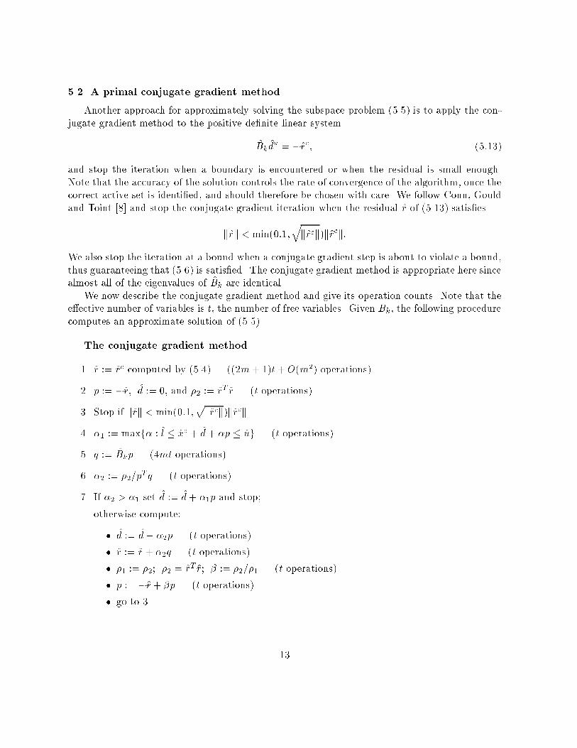
�� A primal conjugate gradient method�

Another approach for approximately solving the subspace problem �� is to apply the con�jugate gradient method to the positive de�nite linear system

�Bk�du � ��rc� ��

and stop the iteration when a boundary is encountered or when the residual is small enoughNote that the accuracy of the solution controls the rate of convergence of the algorithm� once thecorrect active set is identi�ed� and should therefore be chosen with care We follow Conn� Gouldand Toint �� and stop the conjugate gradient iteration when the residual �r of �� satis�es

k�rk � min��qk�rck�k�rck�

We also stop the iteration at a bound when a conjugate gradient step is about to violate a bound�thus guaranteeing that �� is satis�ed The conjugate gradient method is appropriate here sincealmost all of the eigenvalues of �Bk are identical

We now describe the conjugate gradient method and give its operation counts Note that thee�ective number of variables is t� the number of free variables Given Bk � the following procedurecomputes an approximate solution of ��

The conjugate gradient method�

� �r �� rc computed by �� m� ��t�Om�� operations�

� p �� r� �d �� and �� rT �r t operations�

� Stop if k�rk � min��pk�rck�k�rck

� �� maxf� � �l � �xc � �d� �p � �ug t operations�

� q �� Bkp �mt operations�

� �� pTq t operations�

� If �� set �d �� d� ��p and stop�

otherwise compute�

� �d �� d� ��p t operations�

� �r �� r � ��q t operations�

� �� rT �r� � �� t operations�

� p �� r � �p t operations�

� go to �

��

The matrix�vector multiplication of step � should be performed as described in �� The totaloperation count of this conjugate gradient procedure is approximately

�m� ��t� �m� ��t� citer �Om��

where citer is the number of conjugate gradient iterations Comparing this to the cost of theprimal direct method �� it seems that� for t �� m� the direct method is more e�cient unlessciter � m�� Note that the costs of both methods increase as the number of free variables tbecomes larger Since the limited memory matrix Bk is a rank �m correction of the identitymatrix� the termination properties of the conjugate gradient method guarantee that the subspaceproblem will be solved in at most �m conjugate gradient iterations

We should point out that the conjugate gradient iteration could stop at a boundary even whenthe unconstrained solution of the subspace problem is inside the box Consider for example thecase when the unconstrained solution lies near a corner and the starting point of the conjugategradient iteration lies near another corner along the same edge of the box Then the iteratescould soon fall outside of the feasible region This example also illustrates the di�culties thatthe conjugate gradient approach can have on nearly degenerate problems ��

�� A dual method for subspace minimization�

Since it often happens that the number of active bounds is small relative to the size of theproblem it should be e�cient to handle these bounds explicitly with Lagrange multipliers Suchan approach is often referred to as a dual or a range space method see ��

We will writex xk � d�

and restrict xk � d to lie on the subspace of free variables at xc by imposing the condition

ATk d � AT

k xc � xk�

bk�

Recall that Ak is the matrix of constraint gradients� Using this notation we formulate thesubspace problem as

min gkTd� �

�dTBkd ��

subject to ATk d � bk ��

l � xk � d � u� ��

We �rst solve this problem without the bound constraint �� The optimality conditions for�� are

gk �Bkd� �Ak�

� � ��

ATk d

� � bk� ��

��

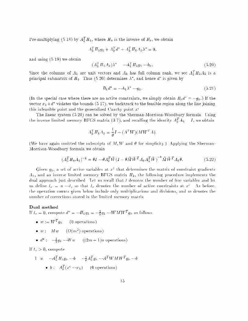
Pre�multiplying �� by ATkHk� where Hk is the inverse of Bk� we obtain

ATkHkgk � AT

k d� �AT

kHkAk��

and using �� we obtainAT

kHkAk�� AT

kHkgk � bk� ��

Since the columns of Ak are unit vectors and Ak has full column rank� we see ATkHkAk is a

principal submatrix of Hk Thus �� determines �� and hence d� is given by

Bkd� � �Ak�

� � gk� ��

In the special case where there are no active constraints� we simply obtain Bkd� � �gk�� If the

vector xk�d� violates the bounds �� we backtrack to the feasible region along the line joiningthis infeasible point and the generalized Cauchy point xc

The linear system �� can be solved by the Sherman�Morrison�Woodbury formula Usingthe inverse limited memory BFGS matrix �� and recalling the identity AT

kAk � I � we obtain

ATkHkAk �

�

I � AT �W � �M �WTA��

We have again omitted the subscripts of M�W and for simplicity� Applying the Sherman�Morrison�Woodbury formula we obtain

ATkHkAk�

�� I � ATk�W I � �M �WTAkA

Tk�W �

�� M �WTAk� ��

Given gk� a set of active variables at xc that determines the matrix of constraint gradientsAk� and an inverse limited memory BFGS matrix Hk� the following procedure implements thedual approach just described Let us recall that t denotes the number of free variables and letus de�ne ta � n � t� so that ta denotes the number of active constraints at xc As before�the operation counts given below include only multiplications and divisions� and m denotes thenumber of corrections stored in the limited memory matrix

Dual method

If ta � �� compute d� � �Hkgk � ��

�gk � �W �M �WT gk as follows

� w �� WTgk � operations�

� w �� Mw Om�� operations�

� d� ��

�gk � �Ww �m� ��n operations�

If ta � �� compute

� u � �ATkHkgk � b � ��

�AT

k gk �AT �W �M �WT gk � b

� b �� ATk x

c � xk� � operations�

��

� v �� WTgk � operations�

� v �� Mw Om�� operations�

� u �� ATk�Wv �mta operations�

� u ��

�AT

k gk � u� b ta operations�

� �� ATkHkAk�

��u � �u � �ATk�W I � �M �WTAkA

Tk�W �

�� M �WTAku

� w �� WTAku �mta operations�

� Form �N � I � �M �WTAkATk�W �

� �N �� WTAkATkW �m� �m�ta operations�

� �N �� I � �M �N Om�� operations�

� w �� N�� Mw Om�� operations�

� �� ATk�Ww �mta operations�

� �� u � �� ta operations�

� d� � �HkAk�� gk� � ��

�Ak�

� � gk�� W �M �WTAk�� v�

� w �� WTAk�� mta operations�

� w �� Mw � v �m operations�

� d� ��

�Ak�

� � gk� � �Ww �m� ��n operations�

Backtrack if necessary�

� Compute �� max f� � li � xc � �xk � d� � xc� � ui� i � Fg t operations�

� Set �x � xc � ��xk � d� � xc� t operations�

Since the vectors STgk and Y T gk have been computed while updating Hk �� they can besaved so that the product �WT gk requires no further computation

The total number of operations of this procedure� when no bounds are active ta � �� is�m� ��n�Om�� If ta bounds are active�

�m� ��n� �mta � �m�ta �Om��

operations are required to compute the unconstrained subspace solution A comparison with thecost of the primal computation implemented as described above� given in �� indicates thatthe dual method would be less expensive when the number of bound variables is much less thanthe number of free variables

However� this comparison does not take into account the devices for saving costs in thecomputation of inner products discussed at the end of x�� In fact� the primal and dual ap�proaches can be brought closer by noting that the matrix I � �

�MWTZZTW �

��M appearing

in �� can be shown to be identical to the matrix I � �M �WTAkATk�W �

�� M in �� If the

��

second expression is used in the primal approach� the cost for the primal computation becomes�m�ta��mt��t�Om�� making it more competitive with the dual approach We have used thisexpression for the primal method in our computational experiments Also� in the dual approach�as with the primal� we save and reuse the inner products in �WTAkA

Tk�W that are relevant for the

next iteration

�� Numerical Experiments

We have tested our limited memory algorithm using the three options for subspace mini�mization the direct primal� primal conjugate gradient and dual methods�� and compared theresults with those obtained with the subroutine SBMIN of LANCELOT �� Both our code andLANCELOT were terminated when

kP xk � gk� l� u�� xkk� � ��

Note from �� that P xk � gk� l� u�� xk is the projected gradient� The algorithm we tested isgiven as follows

L�BFGS�B Algorithm

Choose a starting point x�� and a integer m that determines the number of limited memorycorrections stored De�ne the initial limited memory matrix to be the identity and set k ��

� If the convergence test �� is satis�ed stop

� Compute the Cauchy point by Algorithm CP

� Compute a search direction dk by either the direct primal method� the conjugate gradientmethod or the dual method

� Perform a line search along dk� subject to the bounds on the problem� to compute asteplength �k� and set xk�� xk � �kdk The line search starts with the unit steplength�satis�es �� with � � �� and attempts to satisfy �� with � � ��

� Compute rfxk��

� If yk satis�es �� with eps� �� add sk and yk to Sk and Yk If more than mupdates are stored� delete the oldest column from Sk and Yk

� Update STk Sk� Y T

k Yk � Lk and Rk� and set � yTk yk�yTk sk �

� Set k �� k � � and go to �

The line search was performed by means of the routine of Mor�e and Thuente �� which at�tempts to enforce the Wolfe conditions �� and �� by a sequence of polynomial interpolationsSince steplengths greater than one may be tried� we prevent the routine from generating infeasiblepoints by de�ning the maximum steplength for the routine as the step to the closest bound along

��

the current search direction This approach implies that� if the objective function is boundedbelow� the line search will generate a point xk�� that satis�es �� and either satis�es �� orhits a bound that was not active at xk We have observed that this line search performs well inpractice The �rst implementation of our algorithm used a backtracking line search� but we foundthat this approach has a drawback On several problems the backtracking line search generatedsteplengths for which the updating condition �� did not hold� and the BFGS update had to beskipped This resulted in very poor performance in some problems In contrast� when using thenew line search� the update is very rarely skipped in our tests� and the performance of the codewas markedly better To explore this further we compared the early version of our code� usingthe backtracking line search� with the L�BFGS code for unconstrained optimization �� whichuses the routine of Mor�e and Thuente� on unconstrained problems� and found that L�BFGS wassuperior in a signi�cant number of problems Our results suggest that backtracking line searchescan signi�cantly degrade the performance of BFGS� and that satisfying the Wolfe conditions asoften as possible is important in practice

Our code is written in double precision FORTRAN �� For more details on how to updatethe limited memory matrices in step � see �� When testing the routine SBMIN of LANCELOT �� we tried three options� BFGS� SR� and exact Hessians In all these cases we used the defaultsettings of LANCELOT

The test problems were selected from the CUTE collection �� which contains some problemsfrom the MINPACK�� collection �� All bound constrained problems in CUTE were tested� butsome problems were discarded for one of the following reasons� a� the number of variables was lessthan �� b� the various algorithms converged to a di�erent solution point� c� too many instancesof essentially the same problem are given in CUTE� in this case we selected a representativesample

The results of our numerical tests are given in Tables �� and � All computations wereperformed on a Sun SPARCstation � with a ��MHz CPU and ��MB memory We record thenumber of variables n the number of function evaluations and the total run time The limitedmemory code always computes the function and gradient together� so that nfg denotes the totalnumber of function and gradient evaluations However for LANCELOT the number of functionevaluations is not necessarily the same as the number of gradient evaluations� and in the tables weonly record the number nf� of function evaluations The notation F� indicates that the solutionwas not obtained after �� function evaluations� and F� indicates that the run was terminatedbecause the next iterate generated from the line search was too close to the current iterate to berecognized as distinct This occurred only in some cases when the limited memory method wasquite near the solution but was unable to meet the stopping criterion In Table � nact denotesthe number of active bounds at the solution� if this number is zero it does not mean that boundswere not encountered during the solution process

��

L�BFGS�B L�BFGS�B LANCELOT LANCELOTProblem n nact m�� m�� BFGS SR�

nfg time nfg time nf time nf time

ALLINIT � � ��

BDEXP ��

BIGGS� � � ��

BQPGASIM ��

BQPGAUSS �� F� �� F� �� F� ��

HATFLDA � � ��

HATFLDB � � ��

HATFLDC ��

HS��

HS��

HS��

JNLBRNGA ��

JNLBRNGB ��

LINVERSE �� F� ��

MAXLIKA � � F� �� F� ��

MCCORMCK ��

NONSCOMP ��

OBSTCLAE ��

OBSTCLAL ��

OBSTCLBL ��

OBSTCLBM ��

OBSTCLBU ��

PALMER� � � ��

PALMER� � � F� ��

PALMER� � � F� �� F� ��

PALMER� � � �� F� ��

PROBPENL ��

PSPDOC � � ��

S�� F� ��

TORSION� ��

TORSION� ��

TORSION� ��

TORSION� ��

TORSION� ��

Table � Test results of new limited memory method L�BFGS�B� using primal method forsubspace minimization� and results of LANCELOT�s BFGS and SR� options

��

L�BFGS�B L�BFGS�B L�BFGS�B L�BFGS�BProblem n m�� m�� m�� m��

nfg time nfg time nfg time nfg time

ALLINIT � ��

BDEXP ��

BIGGS� � ��

BQPGASIM ��

BQPGAUSS �� F� �� F� �� F� �� F� ��

HATFLDA � ��

HATFLDB � ��

HATFLDC ��

HS��

HS��

HS��

JNLBRNGA ��

JNLBRNGB ��

LINVERSE ��

MAXLIKA � F� �� F� ��

MCCORMCK ��

NONSCOMP ��

OBSTCLAE ��

OBSTCLAL ��

OBSTCLBL ��

OBSTCLBM ��

OBSTCLBU ��

PALMER� � ��

PALMER� � �� F� ��

PALMER� � �� F� �� F� �� F� ��

PALMER� � F� ��

PROBPENL ��

PSPDOC � ��

S��

TORSION� ��

TORSION� ��

TORSION� ��

TORSION� ��

TORSION� ��

Table � Results of new limited memory method� using the primal method for subspaceminimization� for various values of the memory parameter m

��

L�BFGS�B L�BFGS�B L�BFGS�B LANCELOTProblem n primal dual cg Hessian

nfg time nfg time nfg time nf time

ALLINIT � ��

BDEXP ��

BIGGS� � ��

BQPGASIM ��

BQPGAUSS �� F� �� F� �� F� ��

HATFLDA � ��

HATFLDB � ��

HATFLDC ��

HS��

HS��

HS��

JNLBRNGA ��

JNLBRNGB ��

LINVERSE ��

MAXLIKA � F� �� F� ��

MCCORMCK ��

NONSCOMP ��

OBSTCLAE ��

OBSTCLAL ��

OBSTCLBL ��

OBSTCLBM ��

OBSTCLBU ��


PALMER� � F� �� F� ��

PALMER� � F� �� F� ��


PROBPENL ��

PSPDOC � ��

S��

TORSION� ��

TORSION� ��

TORSION� ��

TORSION� ��

TORSION� ��

Table � Results of new limited memory method using three methods for subspace minimizationprimal� dual and cg�� for m � �� and results of LANCELOT using exact Hessian

��

The di�erences in the number of function evaluations required by the direct primal and dualmethods are due to rounding errors� and are relatively small Their computing time is alsoquite similar due to use of the form described at the end of x�� Our computational experiencesuggests to us that the conjugate gradient method for subspace minimization is the least e�ectiveapproach� it tends to take more time and function evaluations Even though Table � appearsto indicate that the cg option results in fewer failures� tests with di�erent values of m resulted�overall� in three more failures for the cg method than for the primal method The limited memorymethod is sometimes unable to locate the solution accurately� and this can result in an excessivenumber of function evaluations F�� or failure to make further progress F�� The reasons forthis are not clear to us� but are being investigated

The tests described here are not intended to establish the superiority of LANCELOT or ofthe new limited memory algorithm� since these methods are designed for solving di�erent types ofproblems LANCELOT is tailored for sparse or partially separable problems whereas the limitedmemory method is well suited for unstructured or dense problems We use LANCELOT simply asa benchmark� and for this reason ran it only with its default settings and did not experiments withits various options to �nd the one that would give the best results on these problems However�a few observations on the two methods can be made

The results in Table � indicate that the limited memory method usually requires more functionevaluations than the SR� option of Lancelot The BFGS option of Lancelot is clearly inferiorto the SR� option� However in terms of computing time the limited memory method is oftenthe most e�cient� this can be seen by examining the problems with at least �� or �� variableswhich are the only ones for which times are meaningful� To our surprise we observe in Table �that even when using exact Hessians� LANCELOT requires more time than the limited memorymethod on many of the large problems This is in spite of the fact that the objective function inall these problems has a signi�cant degree of the kind of partial separability that LANCELOTis designed to exploit On the other hand� LANCELOT using exact Hessians requires a muchsmaller number of function evaluations than the limited memory method

Taking everything together� the new algorithm L�BFGS�B� has most of the e�ciency of theunconstrained limited memory algorithm L�BFGS� �� together with the capability of handlingbounds� at the cost of a signi�cantly more complex code Like the unconstrained method� thebound limited memory algorithm�s main advantages are its low computational cost per iteration�its modest storage requirements� and its ability to solve problems in which the Hessian matricesare large� unstructured� dense� and unavailable It is less likely to be competitive� in terms offunction evaluations� when an exact Hessian is available� or when signi�cant advantage can betaken of structure However this study appears to indicate that� in terms of computing time� thenew limited memory code is very competitive with all versions of LANCELOT on many problems

A code implementing the new algorithm is described in �� and can be obtained by contactingthe authors at nocedal�eecsnwuedu

��

��

References

�� A V Aho� J E Hopcroft and J D Ullman� The Design and Analysis of Computer Algo�

rithms� Reading� Mass� Addison�Wesley Pub Co� ��

�� B M Averick and J J Mor�e� User guide for the MINPACK�� test problem collection�! Ar�gonne National Laboratory� Mathematics and Computer Science Division Report ANL"MCS�TM�� Argonne� IL� ��

�� DP Bertsekas� Projected Newton methods for optimization problems with simple con�straints!� SIAM J� Control and Optimization ��

�� I Bongartz� AR Conn� NIM Gould� PhL Toint �� CUTE� constrained andunconstrained testing environment!� Research Report� IBM TJ Watson Research Center�Yorktown� USA

�� J V Burke� and J J Mor�e� On the identi�cation of active constraints!� SIAM J� Numer�

Anal� Vol �� No � ��

�� R H Byrd� J Nocedal and R B Schnabel� Representation of quasi�Newton matrices andtheir use in limited memory methods!� Mathematical Programming �� pp ��

�� P H Calamai� and J J Mor�e� Projected gradient methods for linearly constrained prob�lems! Mathematical Programming ��

�� A R Conn� N I M Gould� and PH L Toint� Testing a class of methods for solvingminimization problems with simple bounds on the variables!� Mathematics of Computation�

Vol �� No ��

�� A R Conn� N I M Gould� and PH L Toint� Global convergence of a class of trust regionalgorithms for optimization with simple bounds!� SIAM J� Numer� Anal�� vol ��

�� AR Conn� NIM Gould� PhL Toint �� LANCELOT� a FORTRAN package forlarge�scale nonlinear optimization Release A�!� Number �� in Springer Series in Computa�tional Mathematics� Springer�Verlag� New York

�� AR Conn and J Mor�e� Private communication

�� J E Dennis� Jr and R B Schnabel� Numerical Methods for Unconstrained Optimization

and Nonlinear Equations� Englewood Cli�s� NJ� Prentice�Hall� ��

�� Harwell Subroutine Library� Release �� Advanced Computing Department� AEAIndustrial Technology� Harwell Laboratory� Oxfordshire� United Kingdom

�� JC Gilbert and C Lemar�echal� Some numerical experiments with variable storage quasi�Newton algorithms�! Mathematical Programming ��

��

�� P E Gill� W Murray and M H Wright� Practical Optimization� London� Academic Press��

�� A A Goldstein� Convex programming in Hilbert space!� Bull� Amer� Math� Soc� ��

�� E S Levitin and B T Polyak� Constrained minimization problems!� USSR Comput� Math�

and Math� Phys� � ��

�� D C Liu and J Nocedal� On the limited memory BFGSmethod for large scale optimizationmethods!� Mathematical Programming ��

�� J J Mor�e and DJ Thuente �� On line search algorithms with guaranteed su�cientdecrease!� Mathematics and Computer Science Division Preprint MCS�P�� ArgonneNational Laboratory Argonne� IL�

�� J J Mor�e and G Toraldo� Algorithms for bound constrained quadratic programming prob�lems!� Numer� Math� ��

�� J Nocedal� Updating quasi�Newton matrices with limited storage!� Mathematics of Com�

putation ��

�� JM Ortega and WC Rheinboldt� Iterative Solution of Nonlinear Equations in SeveralVariables!� Academic Press� ��

�� C Zhu� RH Byrd� P Lu and J Nocedal� LBFGS�B� Fortran subroutines for large�scalebound constrained optimization!� Report NAM�� EECS Department� Northwestern Uni�versity� ��

��

NOR THWESTERN UNIVERSITYusers.iems.northwestern.edu/~nocedal/PDFfiles/limited.pdfNOR THWESTERN...

Documents

Transcript of NOR THWESTERN UNIVERSITYusers.iems.northwestern.edu/~nocedal/PDFfiles/limited.pdfNOR THWESTERN...