Nontradable Goods and the Real Exchange Rate · Nontradable Goods and the Real Exchange Rate...

Open Econ RevDOI 10.1007/s11079-012-9250-8

RESEARCH ARTICLE

Nontradable Goods and the Real Exchange Rate

Pau Rabanal · Vicente Tuesta

© Springer Science+Business Media New York 2012

Abstract How important are nontradable goods and distribution costs toexplain real exchange rate dynamics? We answer this question by estimatinga general equilibrium model with intermediate and final tradable and non-tradable goods. We find that the estimated model can match characteristicsof the data that are relevant in international macroeconomics, such as realexchange rate persistence and volatility, and the correlation between thereal exchange rate and other variables. The distinction between tradable andnontradable goods is key to understand real exchange rate fluctuations, butthe introduction of distribution costs is not. Nontradable sector technologyshocks explain about one third of real exchange rate volatility. We also showthat, in order to explain the low correlation between the ratio of relativeconsumption and the real exchange rates across countries, demand shocks arenecessary.

We wish to thank Pablo Guerrón and Carlos Montoro for helpful discussions, and ananonymous referee for very helpful comments. The opinions expressed in this paper arethose of the authors and should not ne attributed to the IMF or IMF policy. Any errorsand omissions are our own. Additional material is available in an online appendix atwww.paurabanal.net/research.html.

P. RabanalInternational Monetary Fund, 700 19th St.,Washington DC, NW 20431, USAe-mail: [email protected]

V. Tuesta (B)CENTRUM Católica, Pontificia Universidad Católica del Perú,Lima, Perue-mail: [email protected]

http://www.paurabanal.net/research.html

P. Rabanal, V. Tuesta

Keywords Real exchange rates · Nontradable goods · Nominal rigidities ·Bayesian estimation

JEL Classification F31 · F32 · F41 · C11

1 Introduction

A main challenge in the empirical international macroeconomics literatureis the so called “real exchange rate disconnect”: models with optimizingagents have difficulty in accounting for the behavior of the real exchangerate. A related problem is that these models are not able to explain keycorrelations between the real exchange rate and other macroeconomic vari-ables. In addition, these models cannot capture the comovement between keymacroeconomic variables across countries. In this paper, we focus on the roleplayed by nontradable goods in explaining the behavior of the real exchangerate.

There is empirical and quantitative evidence supporting the role of nontrad-able goods for to understand real exchange rate dynamics. On the empiricalfront, Betts and Kehoe (2006) provide evidence of the important role ofnontradable goods in accounting for the variance of the real exchange rate ofthe most important U.S. trade partners. They suggest that the larger are tradeflows between two countries, the lower is the importance for deviations fromthe law of one price (i.e. tradable goods prices) for real exchange rate behav-ior. Furthermore, in the U.S., consumption of nontradable goods representsroughly 40 % of GDP and final goods also contain substantial nontradableinput components (between 20 and 30 % of GDP). On the quantitativefront, Stockman and Tesar (1995) show that introducing nontradable goodsin macroeconomic models is crucial to explain international business cycles.More recently, Dotsey and Duarte (2008), Benigno and Thoenissen (2008) andCorsetti et al. (2008) highlight the role of nontradable goods in explaining realexchange rate behavior, and in particular, its persistence and volatility, and itscorrelations with other international relative prices and real variables.

In this paper, we find that nontradable goods play an important role inexplaining real exchange rate dynamics and several international macroeco-nomics facts. Our starting point is an estimated two-country (U.S.-euro area),two-sector (tradable-nontradable goods) dynamic stochastic general equilib-rium (DSGE) model with nominal rigidities, of the class that is now becomingmainstream in academic circles and policy institutions for macroeconomicanalysis.1 Our analysis is empirical and model-based, and we estimate and

1Empirical papers that have estimated fully specified general equilibrium international macroeco-nomic models include Rabanal and Tuesta (2010), Lubik and Schorfheide (2005), Adolfson et al.(2007), Justiniano and Preston (2010) and De Walque et al. (2006). None of the above mentionedstudies consider the role of nontradable goods.


compare two versions of this model: in the first one, the two sectors (tradableand nontradable) produce final consumption goods. In the second one, weintroduce a nontradable intermediate input that is incorporated in the produc-tion of the final tradable good. In this case, we aim at understanding the roleof distribution costs in explaining features of international macroeconomics,as suggested by Dotsey and Duarte (2008). Our methodology consists inestimating each model using a Bayesian approach and eleven macroeconomicseries, including both the producer price index (PPI) for finished industrialgoods and the consumer price index (CPI) for the United States and theEuro Area. PPI inflation (for finished industrial goods) allows us to captureinflation in the tradable goods sector of the economy, and unlike the “goods”component of the CPI, should not include distribution costs. Also, the PPIseries is for finished industrial goods, and hence it should exclude a largerproportion of nontradables than other measures.2

Our results can be summarized as follows. First, the parameter estimates ofthe baseline model are quite similar to what has been estimated or calibratedin the vast existing literature. Therefore, our likelihood-based method doesnot rely on implausible parameter values for structural coefficients such asthe degree of nominal rigidity, the degree of backward looking behavior ininflation or consumption, the monetary policy rules in both countries, and thesize and persistence of economic shocks to explain the data. Second, we findthat the version of the model without distribution costs performs better thanthe version with distribution costs. Since the model already includes severalnominal and real rigidities, the addition of distribution costs does not helpin explaining the data better: in fact, model fit is worse in some dimensions,including real exchange rate persistence. Therefore, our estimates supportthat distribution costs should not be treated differently than other servicesin the production of final goods. Third, our variance decomposition exercise(using the preferred model) shows that the nontradable sector in the modeldoes indeed help to explain real exchange rate fluctuations: nontradable sectortechnology shocks explain as much as 30 % of the fluctuation of the bilateralreal exchange rate, while tradable sector technology shocks and monetarypolicy shocks together explain less than 2 %. Interestingly, demand shocksexplain a great amount of real exchange rate fluctuations (45 %).

Finally, our estimated model allows us to draw important implications forthe behavior of the real exchange rate, the terms of trade and the tradebalance. The relative price of domestic tradables decreases under a tradablesector technology shock, which is consistent with the traditional Balassa-Samuelson effect. With a productivity improvement in either the tradable andnontradable sectors, relative output, consumption and net exports increase. Fi-nally, following a productivity shock in either tradable or nontradable sectors,domestic prices decrease and as a result the real exchange rate depreciates.

2It is impossible to obtain a pure measure of tradable goods inflation. Input-output table data forthe U.S. reveals that services are an intermediate input for the production of industrial goods.


The model features the usual transmission mechanism with terms of tradedeterioration following increases in productivity.3 In addition, our estimatedmodel generates, conditional on a tradable sector productivity shock, a realexchange rate depreciation and an increase in the ratio of relative consump-tions. Therefore, our results suggest that demand shocks are the ones thathelp to explain the negative correlation between the real exchange rate andrelative consumptions observed in the data. On this regard, our findings arein contrast to those of Corsetti et al. (2008), who find that the tradable sectorproductivity shocks are able to explain the apparent lack of risk sharing acrosscountries (negative correlation between relative consumptions and the realexchange rate).

In all the models we estimate, we do not include capital accumulation. Weargue that this is unlikely to change our results. In estimated DSGE modelsthat include investment in the model and in the set of observable variables, aninvestment-specific technology shock is also included (see Rabanal and Tuesta2010). This shock typically explains most of the volatility of investment but italso has counterfactual implications for consumption. In particular, this shockimplies a negative comovement between consumption and investment. Hence,we suspect that if we had introduced investment and investment specific tech-nology shocks, these shocks would not have contributed to explaining RERdynamics and the correlation between consumption and the RER. Moreover,some recent papers have shown that investment-specific technology shocks arenot volatile enough in the data in order to solve certain macroeconomic puzzles(see Mandelman et al. 2011 and Schmitt-Grohe and Uribe 2011). Finally, formost countries it is not possible to obtain data on tradable and nontradableinvestment. Given these concerns and in order to keep the transmissionmechanism simple, we have chosen not to include investment.

The rest of the paper is organized as follows. In Section 2, we present themodel that we estimate. In Section 3 we discuss the data, and the prior andposterior distribution of the model’s parameters. In Sections 4 and 5 we discussthe implications of the estimated model for real exchange rate behavior andthe transmission mechanism in open economies. In Section 6 we discuss theestimation of a model that incorporates distribution services, while Section 7concludes.

2 The Model

In this section, we present the model that we use for analyzing real exchangerate dynamics and the international transmission of shocks. The model isa fairly standard international macro two-country, two-sector (tradable andnontradable) economy, in the spirit of Stockman and Tesar (1995) and Dotsey

3On the contrary, Debaere and Lee (2004), Corsetti et al. (2006) find evidence in support of termsof trade improvement after favorable productivity shocks.


and Duarte (2008). The model includes sticky prices in both sectors, and itassumes that monetary policy is conducted with an interest rate rule of theTaylor type. Based on the arguments by Benigno and Thoenissen (2008) andon the empirical results of Rabanal and Tuesta (2010), we only explore thepossibility that there are incomplete markets at the international level. Finally,we assume that the law of one price holds and intermediate firms set prices intheir own currency.4

Since our contribution is to estimate this model using Bayesian methodsand eleven observable variables, in this section we briefly present its mainassumptions, parameters and functional forms, and refer the reader to theonline appendix for a full-blown version of the model. In the last sectionof the paper, we study the effects of introducing a distribution sector in themodel. We follow Dotsey and Duarte (2008) and assume that the productionfunction of final tradable goods includes a portion of nontradable inputs.Finally, to keep the exposition of the model at its minimum, we only presentthe equations for households and firms in the home country. The expressionsfor the foreign country are analogous, and obtaining them is straightforward,with the appropriate change of notation.5

Households Representative households in the home country are assumed tomaximize the following utility function:

Ut = E0

{ ∞∑t=0

β tψt

[log(Ct − bCt−1

)− L1+ϕt

1 + ϕ

]}, (1)

subject to the following budget constraint:

BHt

Pt Rt+ St BF

t

Pt R∗t �(

St BFt

PtYt

) ≤ BHt−1

Pt+ St BF

t−1

Pt+ Wt

PtLt − Ct + �t. (2)

E0 denotes the conditional expectation on information available at date t = 0,

β is the intertemporal discount factor, with 0 < β < 1. Ct denotes the level ofconsumption in period t, Lt denotes labor supply. The utility function displaysexternal habit formation with respect to the habit stock, which is last period’saggregate consumption of the economy Ct−1. b ∈ [0, 1] denotes the importanceof the habit stock. ϕ > 0 is inverse elasticity of labor supply with respect to thereal wage. ψt is a preference shock that follows a zero-mean AR(1) process inlogs:

log ψt = ρψ log ψt−1 + εψt . (3)

4Dotsey and Duarte (2008) show that alternative assumptions regarding pricing decisions of firms,namely producer currency pricing (PCP) and local currency pricing (LCP), are not so different forthe real exchange rate dynamics.5The convention will be to use an asterisk to denote the counterpart in the foreign country of avariable in the home country (i.e. if aggregate consumption is C in the home country, it will beC∗ in the foreign country and so on. The same applies to the model’s parameters. When there ispotential for confusion we explictly clarify so.


In the budget constraint, Wt is the nominal wage, Pt is the consumer priceindex, and �t are real profits for the home consumer. For modelling simplicity,we choose to assume incomplete markets at the international level with tworisk-free one-period nominal bonds denominated in domestic and foreigncurrency, and a cost of bond holdings is introduced to achieve stationarity(see Benigno 2009). BH

t is the holding of the risk free domestic nominal bondand BF

t is the holding of the foreign risk-free nominal bond expressed inunits of foreign country currency. St is the nominal exchange rate, expressedin units of home country currency per unit of foreign country currency. Rt

and R∗t are the nominal interest rates in the home and foreign countries. The

function �(.) depends on the aggregate net foreign asset position of the homecountry, BF

t , in percent of home-country GDP, and is taken as given by thedomestic household. �(.) is a convex function that introduces the cost ofundertaking positions in the international asset market, and allows to have awell-defined steady-state. In addition, it is assumed that � (0) = 1 and that �(.)

is a decreasing function. Also, while we do not make it explicit in the budgetconstraint 2, we assume that there are complete markets at the domestic level,such that the consumption/savings decision is the same among households ina country, and the stochastic discount factor to value future profits is also thesame among households in a country.

The aggregate consumption index (Ct) is a composite of final tradable (CTt )

and final nontradable (CNt ) consumption goods. We define the consumption

index as

Ct ≡[γ 1/ε

c

(CT

t

) ε−1ε + (1 − γc)

1/ε(CN

t

) ε−1ε

] εε−1

, (4)

where ε is elasticity of substitution between the final tradable (CTt ) and final

nontradable (CNt ) goods, and γc is the share of final tradable goods in the

consumption basket at home. In this context, the consumer price index thatcorresponds to the previous specification is given by

Pt ≡[γc(PT

t

)1−ε + (1 − γc)(PN

t

)1−ε] 1

1−ε

, (5)

where all prices are for goods sold in the home country, in home currency andat the consumer level, for both tradable and nontradable goods.

The demand functions for the final tradable and nontradable goods aregiven by:

CTt = γc

(PT

t

Pt

)−ε

Ct, and CNt = (1 − γc)

(PN

t

Pt

)−ε

Ct, (6)

while consumption/savings decisions in home and foreign bonds are standard:

λt = βEt

{Rt

Pt

Pt+1λt+1

}, (7)

λt = �

(St BF

t

PtYt

)βEt

{R∗

tQt+1

Qtλt+1

}, (8)


where λt = ψt

Ct−bCt−1is the marginal utility of consumption, and Qt = St P∗

tPt

is thereal exchange rate. Labor supply is given by:

λtWt

Pt= Lϕ

t . (9)

Firms There are three sectors in each country: (i) a final goods producersector, that produces final tradable and nontradable goods for consumption bydomestic households, (ii) an intermediate tradable goods sector, that producesgoods that can be traded internationally to final tradable goods producerseither in the home or in the foreign country, and (iii) an intermediate nontrad-able goods sector, that sells its production to final nontradable goods produc-ers. We assume that the final goods producers operate under flexible pricesand perfect competition, while intermediate goods producers operate understicky prices à la Calvo with partial indexation, and monopolistic competition.

Final Goods Producers The final tradable good is consumed by domestichouseholds. This good is produced by a continuum of firms, each producingthe same variety, labelled by YT

t , using intermediate home(Xh

t

)and foreign(

X ft

)goods with the following technology:

YTt =

{γ 1/θ

x

(Xh

t

) θ−1θ + (1 − γx)

1/θ(

X ft

) θ−1θ

} θθ−1

, (10)

where θ is the elasticity of substitution between home-produced and foreign-produced imported intermediate goods. Xh

t and X ft denote the amount of

home and foreign intermediate tradable inputs to produce the final tradablegood at home, are also Dixit-Stiglitz aggregators of all types of home andforeign intermediate goods, with elasticity of substitution σ .:

Xht ≡

[∫ 1

0Xh

t (h)σ−1σ dh

] σσ−1

, and X ft ≡

[∫ 1

0X f

t ( f )σ−1σ df

] σσ−1

.

Optimizing conditions by final tradable goods producers deliver the followingdemand functions:

Xht (h) = γx

(Ph

t (h)

Pht

)−σ (Ph

t

PTt

)−θ

YTt , and

X ft ( f ) = (1 − γx)

(P f

t ( f )

P ft

)−σ (P f

t

PTt

)−θ

YTt , (11)

where

Pht ≡

[∫ 1

0Ph

t (h)1−σ dh] 1

1−σ

, P ft ≡

[∫ 1

0P f

t ( f )1−σ df] 1

1−σ

.


Thus, the price index of tradable goods is given by:

PTt =

[γx(Ph

t

)1−θ + (1 − γx)(

P ft

)1−θ] 1

1−θ

. (12)

We assume that the law of one price holds for intermediate inputs, such thatPh

t (h) = Ph∗t (h)St, and P f

t ( f ) = P f ∗t ( f )St.

The production of the final nontradable good is given by:

Y Nt ≡

[∫ 1

0X N

t (n)σ−1σ dn

] σσ−1

where we assume the same elasticity σ > 1 than in the case of final tradablegoods produced in the home country. The price level for nontradables is

PNt ≡

[∫ 1

0pN

t (n)1−σ dn] 1

1−σ

Intermediate Goods Producers The structure of intermediate goods produc-ers in the two sectors is very similar. The main difference is that the inter-mediate nontradable sector produces differentiated goods that are aggregatedby final nontradable good producing firms, and ultimately used for finalconsumption by domestic households only, while the intermediate tradablesector produces differentiated goods that can be sold to home and foreign finaltradable good producers.

The production function in both sectors is linear in the labor input and hastwo technology shocks:

Y Nt (n) = At Z N

t LNt (n), for n ∈ [0, 1], and

Yht (h) = At Z h

t Lht (h), for h ∈ [0, 1] (13)

where At is a labor augmenting aggregate world technology shock which has aunit root with drift:

log At = g + log At−1 + εat (14)

Hence, real variables in both countries grow at a rate g. Z Nt and Z h

t arecountry-specific, stationary productivity shocks to the nontradable and thetradable sector at time t, which evolve according to zero-mean, AR(1) processin logs

log Z Nt = ρZ ,N log Z N

t−1 + εZ ,Nt , and log Z h

t = ρZ ,h log Z ht−1 + ε

Z ,ht (15)

Firms in both sectors face a Calvo lottery with partial indexation when settingtheir prices. In the nontradable sector, firms receive a stochastic signal thatallows them to reset prices optimally in each period, with probability 1 − αN .We assume that there is partial indexation with a coefficient ϕN to last period’s


sectorial inflation rate for those firms that do not get to reset prices optimally.As a result, firms maximize the following profits function:

MaxPNt (n)Et

∞∑k=0

αkN�t,t+k

⎧⎪⎨⎪⎩⎡⎢⎣ PN

t (n)(

PNt+k−1

PNt−1

)ϕN

Pt+k− MCN

t+k

⎤⎥⎦Y N,d

t+k (n)

⎫⎪⎬⎪⎭ (16)

subject to

Y N,dt+k (n) =

[(PN

t (n)

PNt+k

)(PN

t+k−1

PNt−1

)ϕN]−σ

Y Nt (17)

where Y N,dt (n) is total individual demand for a given type of nontradable good

n, and Y Nt is aggregate demand for nontradable goods, as defined above, and

�t,t+k = βk λt+kλt

is the stochastic discount factor. MCNt corresponds to the real

marginal cost in the nontradable sector. From cost minimization:

MCNt = Wt

Pt Z Nt At

(18)

The evolution of the price level of nontradables is

PNt ≡

{αN

[PN

t−1

(�N

t−1

)ϕN]1−σ + (1 − αN)

(pN

t

)1−σ} 1

1−σ

(19)

where �Nt−1 = PN

t−1

PNt−2

. Similar expressions hold for the intermediate tradable

sector, where the relevant parameters for price setting are αh and ϕh, andwith the appropriate change of notation in Eqs. 16, 17, 18, and 19, and similarexpressions hold for the foreign country.

Closing the Model The model includes a demand shock. One interpretationis that this shock is a government spending shock that is financed by lump-sum taxation. More generally, this demand shock is capturing movementsin GDP and in consumption that cannot be explaining through interest-ratechanges. Hence, we will be using both terms: demand shock and governmentspending shock, to refer to the shock in the market clearaing condition. Weassume that the demand shock is allocated between tradable and nontradablegoods in the same way that private consumption is. Hence the market clearingconditions for both types of final goods, consisting of private consumption andgovernment spending, are:

YTt = CT

t + GTt , (20)

and

Y Nt = CN

t + GNt , (21)


where GNt , GT

t follow AR(1) processes in logs. The bond market clearingconditions are:

BHt + BH∗

t = 0, (22)

and

BFt + BF∗

t = 0. (23)

For the nontradable intermediate goods, the market clearing condition is:

Y Nt (n) = X N

t (n), for all n ∈ [0, 1],while for the intermediate tradable goods sector it is:

Yht (h) = Xh

t (h) + Xh∗t (h), for all h ∈ [0, 1].

Monetary policy is conducted with a Taylor rule that targets CPI inflation andoutput growth deviation from steady-state values:

Rt = R(1−ρr) Rρrt−1

(Pt/Pt−1

�

)(1−ρr)γπ(

Yt/Yt−1

1 + g

)(1−ρr)γy

exp(εrt ). (24)

3 Data, Priors and Posterior Distributions

We use Bayesian methods to estimate the parameters of the model ofSection 2. Bayesian estimation of DSGE models has now become very popular,so we leave the technical details and a discussion of its benefits aside.6 Weuse the following data series for each country: output (real GDP) growth percapita, consumption growth per capita, CPI inflation, interest rates on 3-monthT-Bills, and PPI inflation for finished industrial goods. CPI inflation is usedas a measure of overall inflation, while PPI inflation tries to measure theinflation in the tradable sector of the economy. Several authors (Engel 1999;Betts and Kehoe 2006) have emphasized that using the “goods” componentof the CPI might not be a good proxy for tradable goods, because it containsdistribution and retail services that are nontradable. The home country is theeuro area, and the foreign country is the U.S. The last series that we use inthe estimation procedure is the bilateral real exchange rate between the euroand the US dollar. To construct this series, we multiply the nominal exchangerate (in euros per U.S. dollar) by the U.S. CPI, and divide it by the euro areaCPI. An increase of the real exchange rate is an euro depreciation. Theseeleven variables are our set of observable variables in the likelihood function.The sample period goes from 1985:02 to 2004:04. We are constrained by theavailability of the PPI series for finished industrial goods in the euro area, sinceall other variables are available from earlier periods.

6See An and Schorfheide (2007), Lubik and Schorfheide (2005) and Fernandez-Villaverde andRubio-Ramírez (2004) for detailed explanations on how to implement a Bayesian approach toestimation of fully-specified dynamic stochastic general equilibrium models.


Before we proceed to describe the prior and posterior distribution of themodel’s parameters, we discuss what parameters we calibrate first. We followDotsey and Duarte (2008) closely, and calibrate the two economies with thesame parameters. We set the share of tradable goods in the CPI to γc = 0.44.We set the fraction of intermediate tradable inputs in the production of finaltradable goods to γx = 0.6. Since we are not using labor market data wecalibrate the value of ϕ = 1, which is in line with parameter estimates obtainedby Rabanal and Rubio-Ramírez (2005, 2008). We set the steady-state growthrate of the economy, g, equal to 0.5 %, which implies that the world growthrate of per capita variables is about 2 % per year. In order to match a realinterest rate in the steady state of about 4 % per year, we set the discountfactor to β = 0.99. For reasonable parameterizations of these two variablesthe parameter estimates do not change significantly. Finally, the parameter χ ,that measures the elasticity of the risk premium with respect to the net foreignasset position, is set equal to 0.007 based on Rabanal and Tuesta (2010).

With the previous parameters fixed in advance, Table 1 presents the priorand posterior distributions for the model’s remaining parameters which arefairly standard (see Smets and Wouters 2003; Lubik and Schorfheide 2005 andRabanal and Tuesta 2010). In order to make the table more readable, we alsoinclude a brief description of each parameter.

Since we are mostly interested in understanding the implications of themodel for real exchange rate dynamics and the international transmissionof shocks, we briefly comment on the parameter estimates. Overall, theyare quite similar to what has been obtained in the literature that estimatesopen economy dynamic macroeconomic models with Bayesian methods.7 Theestimates for the degree of habit formation are quite similar in both countries,of 0.57 in the United States and of 0.58 in the euro area, respectively. Theelasticity of substitution between home and foreign tradable inputs, θ, isestimated at 0.85, a value much smaller than the prior mean of 1.5, whichwas chosen according to Chari et al. (2002). However, this value is higherthan that obtained by Rabanal and Tuesta (2010) and Lubik and Schorfheide(2005) in a model with tradable goods only. As it will become clearer later, thehigher estimated value for this elasticity stems from endogenous volatility thatnontradable goods adds to the model, hence making less necessary a smallvalue of θ to account for real exchange volatility. On the other hand, theelasticity of substitution between tradable and nontradable final consumptiongoods, ε, is estimated to be quite low, with a posterior mean of 0.13, which ismuch lower than the prior mean, of 1, and the value typically used calibratedexercises in the literature of 0.44, following Stockman and Tesar (1995). Theestimated Phillips Curves suggest that prices in the U.S. are reset optimallyabout every 2 quarters in both sectors, with a low degree of backward lookingindexation (ϕN∗ , ϕ f ∗), between 0.06 in the nontradable sector and 0.21 in thetradable sector. The Phillips Curves in the euro area are more heterogeneous:

7See Lubik and Schorfheide (2005) and Rabanal and Tuesta (2010).


Table 1 Prior and posterior distributions

Prior PosteriorDistribution Mean St.Dev Mean Lower Upper

Habit formationb EMU Beta 0.70 0.05 0.57 0.51 0.64b∗ USA Beta 0.70 0.05 0.58 0.52 0.64

Elasticities of substitutionθ Home and foreign tradable Normal 1.50 0.25 0.85 0.80 0.93

int. goodsε Tradable and nontradable Gamma 1.00 0.25 0.13 0.09 0.18

final goodsCalvo parameters

αh Tradable int. goods EMU Beta 0.50 0.20 0.73 0.66 0.80α f ∗ Tradable int. goods USA Beta 0.50 0.20 0.48 0.38 0.59αN Nontradable int. goods EMU Beta 0.50 0.20 0.10 0.03 0.17αN∗ Nontradable int. goods USA Beta 0.50 0.20 0.40 0.34 0.46

Indexation parametersϕh Tradable int. goods EMU Beta 0.50 0.20 0.30 0.07 0.51ϕ f ∗ Tradable int. goods USA Beta 0.50 0.20 0.21 0.01 0.41ϕN Nontradable int. goods EMU Beta 0.50 0.20 0.39 0.08 0.69ϕN∗ Nontradable int. goods USA Beta 0.50 0.20 0.06 0.01 0.10

Taylor rule coefficientsρr Interest rate smoothing EMU Unif orm 0.50 0.29 0.76 0.71 0.82ρr∗ Interest rate smoothing USA Unif orm 0.50 0.29 0.88 0.85 0.90γπ Response to inflation, EMU Normal 1.50 0.25 2.72 2.46 2.98γπ∗ Response to inflation, USA Normal 1.50 0.25 2.05 1.73 2.34γy Response to growth, EMU Normal 1.00 0.25 0.56 0.40 0.71γy∗ Response to growth, USA Normal 1.00 0.25 0.91 0.68 1.15

Prior and posterior distributions of shock

AR coefficientsPreference

ρψ EMU Beta 0.75 0.10 0.87 0.82 0.92ρψ∗ USA Beta 0.75 0.10 0.88 0.83 0.93

TechnologyρZ ,h Tradable int. sector EMU Beta 0.75 0.10 0.94 0.89 0.98ρZ , f ∗

Tradable int. sector USA Beta 0.75 0.10 0.93 0.88 0.98ρZ ,N Nontradable int. sector EMU Beta 0.75 0.10 0.97 0.95 0.99ρZ ,N∗

Nontradable int. sector USA Beta 0.75 0.10 0.93 0.90 0.97Government spending

ρG,T Tradable sector EMU Beta 0.75 0.10 0.84 0.75 0.94ρG,T∗

Tradable sector USA Beta 0.75 0.10 0.73 0.56 0.89ρG,N Nontradable sector EMU Beta 0.75 0.10 0.85 0.76 0.94ρG,N∗

Nontradable sector USA Beta 0.75 0.10 0.93 0.89 0.97Standard deviations of shocks (in percent)

Preferenceεψt EMU Gamma 1.00 0.50 1.89 1.43 2.36

εψ∗t USA Gamma 1.00 0.50 1.91 1.50 2.30

TechnologyεZ ,h Tradable int. sector EMU Gamma 0.70 0.30 1.38 1.06 1.71εZ , f ∗

Tradable int. sector USA Gamma 0.70 0.30 1.72 1.37 2.05εZ ,N Nontradable int. sector EMU Gamma 0.70 0.30 1.81 1.54 2.08εZ ,N∗

Nontradable int. sector USA Gamma 0.70 0.30 1.02 0.82 1.22εa Permanent technology shock. Gamma 0.70 0.30 0.36 0.19 0.53


Table 1 (continued)

Prior PosteriorDistribution Mean St.Dev Mean Lower Upper

Government spendingεG,T Tradable sector EMU Gamma 1.00 0.50 1.00 0.45 1.65εG,T∗

Tradable sector USA Gamma 1.00 0.50 0.69 0.15 1.22εG,N Nontradable sector EMU Gamma 1.00 0.50 3.05 2.68 3.46εG,N∗

Nontradable sector USA Gamma 1.00 0.50 4.07 3.57 4.60Monetary policy

εr EMU Gamma 0.40 0.20 0.16 0.12 0.19εr∗

USA Gamma 0.40 0.20 0.11 0.09 0.13

the estimated probability of not resetting prices is 0.73 in the tradable sector,while we obtain a surprisingly low coefficient for the nontradable sector, wherethe posterior mean is 0.1, much lower than the prior mean of 0.5. Backwardlooking behavior is higher than in the case of the U.S., with coefficients of 0.3in the tradable sector and 0.4 in the nontradable sector. Finally, the coefficientsof the Taylor rule are quite similar to previous estimates in the literature for thesample period that we use, starting in 1985, with coefficients on the responseof nominal interest rates to inflation of 2 in the United States (Clarida et al.2000) and even higher in the euro area. Regarding the exogenous processes,all shocks are estimated with high, but reasonable, persistence. The technologyshock in the intermediate nontradable sector has the highest persistence, witha posterior mean of 0.97, while the persistence of all the other shocks rangesbetween that value and 0.73 for the demand shock in the tradable sector inthe U.S. The high persistence in preference and technology shocks in thenontradable sector in U.S. might explain why the backward behavior in pricesetting is unimportant. Similar results have been found by Ireland (2006) foran estimated closed economy using U.S. data.

4 Implications for Real Exchange Rate Dynamics: Second Momentsand Variance Decomposition

After taking a linear approximation of the equilibrium conditions around thesteady state, the equations determining the real exchange rate are as follows.First, combining the consumption Euler equations for both households, weobtain that:

Et (qt+1 − qt) =[(1 + g) Et�ct+1 − b�ct

(1 + g − b)

]−[(1 + g) Et�c∗

t+1 − b ∗�c∗t

(1 + g − b ∗)

]

+ (1 − ρψ

)ψt − (1 − ρ∗

ψ

)ψ∗

t + χb t (25)

where qt is the real exchange rate, ct and c∗t are consumption in the euro area

and in the United States, b t =(

St BFt

Pt

)Y−1 is the net foreign asset position

as percent of GDP, where χ ≡ −�′ (0) Y, and ψt and ψ∗t are the preference


shocks (all expressed in log deviations from steady-state values).8 Therefore,in principle, if consumption growth in both areas is not related to the realexchange rate, the preference shocks should allow us to explain the data in caseof misspecification. In addition, by taking the definition of the real exchangerate as the ratio of price levels expressed in common currency, and by using thedefinition of the CPIs in both countries and the definitions of the price level oftradable goods, we obtain the following expression:

qt = (2γx − 1)tt + (1 − γc)[(tTt − tN

t ) − (tT∗t − tN∗

t )] (26)

where tt is the terms of trade, defined as the price of imports minus the priceof exports, ti

t = pit − pt, i = T, N is the relative price between tradables and

nontradables in the euro area CPI, and ti∗t = pi∗

t − p∗t , i = T, N is the relative

price between tradables and nontradables in the U.S. CPI. Therefore, theshocks that drive the terms of trade, or that move prices of tradable andnontradable goods in both countries in different directions, are also likelyto affect the behavior of the real exchange rate. Indeed, the presence ofnontradable goods helps in breaking the strong correlation between the realexchange rate and the terms of trade implied by a model without nontradablegoods: In that particular case, γc = 1, and qt = (2γx − 1)tt. Furthermore, aspointed out by Dotsey and Duarte (2008), the presence of nontradable goodslowers the correlation of real variables with international relative prices,helping the model to better explain the data. In the next sub-section we analyzesome second moments and evaluate how well the estimated model works in theprevious mentioned dimensions.

In the Bayesian approach, assessments of the goodness of fit and modelcomparisons are performed using the marginal likelihood of the data, whichupdates the researcher’s prior beliefs on which model is closer to the trueone after observing the data. Fernandez-Villaverde and Rubio-Ramírez (2004)show that, in the Bayesian framework, model comparison is consistent whenmodels are misspecified, which is typically the case. However, the marginallikelihood, which averages all possible likelihood values implied by the modelacross the parameter space, using the prior as a weight, is a summary statisticof overall goodness of fit. In this section, we focus instead on a subset ofsecond moments that are key in the international macroeconomics literature.In Table 2 we present some selected posterior second moments of the raw data,while in Table 3 we report selected posterior second moments of HP-filteredreal variables.

The model overpredicts the volatility of consumption and output growth,and of CPI and PPI inflation in both countries, while it underpredicts thevolatility of nominal interest rates and the real exchange rate (Table 2). Yet,using a longer period that includes the 1970s makes the model fit the inflation

8The evolution of net foreign assets over GDP is: βb t = 11+g b t−1 + X f

Y

(xh∗

t − x ft − tt

)where X f

Y

is the imports-GDP ratio, xh∗t is exports of intermediate tradable goods, x f

t is imports, and tt is theterms of trade. Appendix B details the full set of loglinearized conditions of the model.


Table 2 Second moments in the model and in the data

Euro area United States

Y C R CPI PPI Y C R CPI PPI Q

Standard Deviation (in %)Data 0.51 0.51 0.77 0.27 0.33 0.50 0.48 0.49 0.36 0.79 4.64Model 0.74 0.87 0.57 0.55 0.60 0.59 0.75 0.49 0.84 1.23 3.34

Variance decompositionPreferences 9.6 11.0 68.3 25.3 19.8 4.1 13.2 65.9 43.5 14.4 23.6Tech. tradable 7.4 8.4 4.3 4.1 52.9 11.9 14.0 5.0 12.1 63.8 0.9Tech. nontradable 49.5 56.5 19.2 33.4 18.3 20.4 55.9 22.7 23.7 13.1 31.8Demand shock 26.4 19.5 7.1 16.8 5.5 51.8 10.4 5.8 4.7 2.9 43.5Monetary policy 0.2 0.2 0.3 16.2 3.1 0.8 1.2 0.5 14.3 5.1 0.2Unit root Shock 7.0 4.4 0.9 4.3 0.3 11.0 5.4 0.1 1.6 0.8 0.1

Note: Y is output, C is consumption, R is nominal interest rate. Q is the real exchange rate.Moments for R are based on the level of this variable, in all other cases they are based on theirquarterly growth rate

data better as documented by Rabanal and Tuesta (2010). To explain whichshocks drive the behavior of macroeconomic variables, we perform a variancedecomposition exercise and then add up shocks across countries.9 Most im-portant for the purpose of this paper, we examine what is the role of eachshock in explaining real exchange rate fluctuations. In this case, demand shocks(mostly in the tradable sector, not shown) explain 43.5 % of the variance of thereal exchange rate, while technology shocks in the nontradable sector explain31.8 %, and preference shocks explain 23.6 %. The other shocks (monetarypolicy, innovations to the permanent technology shock, and the tradable sectortechnology shock) explain about the remaining 1 %. These results confirm thefindings of Rabanal and Tuesta (2010) with a model with tradable goods only.Of course, in that case we were not able to tell what sector the shocks belongedto, but we assigned an important contribution (about 40 % each) to technologyand demand factors. In the present estimated model, nontradable technologyshocks, fiscal shocks and preference shocks are able to explain a large fractionof the volatility of most variables. Note also that the tradable sector technologyshocks only explain an important fraction of tradable (PPI) inflation in bothcountries. Therefore, shocks arising in the nontradable sector are an impor-tant source of real exchange rate fluctuationsFinally, the monetary policyshock does explain a significant fraction of CPI inflation in both countries,about 15 %.

As suggested by Table 3, the model does a good job in explaining the inter-national dimension of the data, in particular to the relationship of output acrosscountries and the correlation between relative output and the real exchangerate. The model is also able to explain the so-called consumption-real exchange

9That is, the contribution of the “Preference” shock adds up the contribution of the euro area andthe U.S. preference shock. The only exception is the demand shock for which we have aggregatedacross countries and sectors.


Table 3 Second moments in the model and in the data

Correlation Y,Y* C,C* C-C*,Q Y-Y*,Q Q,Q−1

Data 0.30 0.18 0.01 0.15 0.78Model 0.36 −0.28 0.05 0.20 0.78

Preferences 0.85 −0.70 −0.97 −0.96 0.77Tech. tradable 0.96 0.87 0.84 0.89 0.62Tech. nontradable 0.12 −0.49 0.89 0.91 0.77Demand shocks 0.29 −0.55 −0.90 −0.38 0.79Monetary policy 0.95 0.91 0.81 0.85 0.23Unit root shock 1.00 1.00 0.78 −0.61 0.18

Note: Y is output, C is consumption, Q is the real exchange rate. All moments are computed bysimulating the model 1,000 times with 85 periods at the posterior mean and applying the HP filter

rate anomaly. In the sample period that we use, the correlation between theratio of relative consumptions and the real exchange rate is basically zero.10

The fact that the model can match a basically zero correlation should not maskthat the transmission mechanisms underlying this result are very different.While technology shocks in both sectors, monetary policy and unit root shocksdeliver a high and positive correlation between these two variables, preferenceand demand shocks deliver a highly negative correlation. Therefore, anymodel that tries to be successful in explaining this correlation must have acombination of the two, even when the model includes nontradable goods. Thesame result applies when studying the correlation between relative outputs andthe real exchange rate. Finally, we would like to remark that the model is ableto fit real exchange rate persistence, with a first autocorrelation in the HP-filtered real exchange rate in the model and in the data of 0.78. Also, the threeshocks that explain most of real exchange rate volatility are able to explain itspersistence.11

5 Implications for the Transmission Mechanism

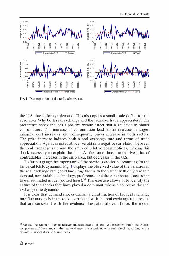
Having shown what are the three shocks that explain the behavior of the realexchange rate in the previous section, we now turn to discuss the impulseresponses to a nontradable technology shock, a tradable sector demand shock,and a preference shock in the euro area. In Fig. 1 we depict the effects of a

10Adding the seventies and mid-eighties sample, as in Rabanal and Tuesta (2010), delivers anegative correlation of −0.17, that a model with incomplete markets and tradable goods can match.11We use HP-filtered data to be able to compare our results with the international real businesscycle literature, including Corsetti et al. (2008). The empirical literature interpreted real exchangerate persistence as the slow rate of mean reversion of the real exchange rate. Early examplesof applications include Rogoff (1996) and the references therein. A typical result is the strongevidence of slow mean reversion, found by estimating first order autoregressive models for thelevel of the exchange rate instead of using HP filtered data. For a recent application, see Steinsson(2008).


1 2 3 4 5 6 7 8 9 10-1

0

1

2

3

4

5

6

7

8x 10-3

Pct

. Dev

. Ste

ady

Sta

te

Quarters After Shock

Y EMUY USARELATIVE Y

1 2 3 4 5 6 7 8 9 10-0.01

-0.005

0

0.005

0.01

0.015

0.02

Pct

. D

ev.

Ste

ady

Sta

te


C EMUC USARELATIVE C

1 2 3 4 5 6 7 8 9 100

0.002

0.004

0.006

0.008

0.01

0.012

0.014

0.016

0.018

Pct

. Dev

. Ste

ady

Sta

te


RERTOTNX

1 2 3 4 5 6 7 8 9 10-0.02

-0.015

-0.01

-0.005

0

0.005

0.01

0.015

Pct

. Dev

. Ste

ady

Sta

te


REL N EMUREL N USA

Fig. 1 Impulse response to a nontradable technology shock in the euro area

positive (one standard deviation) nontradable sector technology shock. As aresult, consumption and output increase in the euro area. The real exchangerate and the terms of trade depreciate following the shock, and the relativeprice of nontradables (RELN = PN

PT ) falls in the euro area where as it increasesin the USA. From Eq. 26, the RER dynamics can be decomposed in the terms-of-trade effect, (2γx − 1) tt, and the movements of relative prices of tradable tonontradable goods in both countries. We can further rearrange Eq. 26 to get:

qt = (2γx − 1)tt + (1 − γc)(relN∗t − relN

t )

where relNt = pN

t − pTt and relN∗

t = pN∗t − pT∗

t . In this case, both relative-priceeffects move the real exchange rate in the same direction. The terms of tradedepreciate because of the associated nominal exchange rate depreciation ofthe euro. This causes consumption to fall in the U.S., and also the relativeprice of tradable goods to increase. Finally, there is a small improvementof the trade balance but of several orders of magnitude smaller than allother variables. With an estimated θ close to one, the trade balance barelymoves in all the exercises that we show, because real quantities offset themovements in real prices. This shock implies a positive correlation betweenboth the real exchange rate and the terms of trade with both relative outputand consumption. The impulse response to a tradable sector technology shock(not shown) displays similar behavior of the main variables, except for the


1 2 3 4 5 6 7 8 9 10-4

-3.5

-3

-2.5

-2

-1.5

-1

-0.5

0x 10-3

Pct

. D

ev.

Ste

ady

Sta

te



1 2 3 4 5 6 7 8 9 10-7

-6

-5

-4

-3

-2

-1

0

1

2x 10-3

Pct

. D

ev.

Ste

ady

Sta

te



1 2 3 4 5 6 7 8 9 10-0.005

0

0.005

0.01

0.015

0.02

0.025

Pct

. D

ev.

Ste

ady

Sta

te


RERTOTNX

1 2 3 4 5 6 7 8 9 10-0.015

-0.01

-0.005

0

0.005

0.01

0.015

0.02

0.025

0.03

Pct

. D

ev.

Ste

ady

Sta

te


REL N EMUREL N USA

Fig. 2 Impulse response to a tradable demand shock in the euro area

relative prices of nontradable to tradable goods.12 Our estimated impulseresponses are in line with those reported by Dotsey and Duarte (2008) usinga calibrated model for the U.S. and OECD countries. However, our empiricalresults challenge those of Corsetti et al. (2006) which find exactly the opposite.

Figure 2 displays the impulse response to a demand shock in the tradablesector in the euro area. In this case, consumption declines in the euro areaand increases in the U.S., while the euro depreciates in real terms. The termsof trade also depreciates which boosts consumption in U.S. Why do both thereal exchange rate and the terms of trade depreciate? Since the model features,infinitely-lived Ricardian households, the positive demand shock (which worksas a fiscal shock) induces a negative wealth effect in euro area: agents workmore and consume less today. Hence, the labor supply increases, causing areduction in real wages that translates into a reduction in marginal costs inboth sectors. Thus, domestic prices (tradable and nontradable) decrease, whichtriggers both a real exchange rate and terms of trade depreciation.

The ratio of relative consumptions decreases with the depreciation, and im-plies a strong negative correlation between the real exchange rate and relativeconsumptions across countries. Negative wealth effects cause consumption to

12For robustness, we have also performed an estimation using the terms of trade as an observablevariable. Qualitatively, the impulse-responses do not change. Results are available upon request.


1 2 3 4 5 6 7 8 9 100

0.5

1

1.5

2

2.5x 10-3

Pct

. D

ev.

Ste

ady

Sta

te



1 2 3 4 5 6 7 8 9 10-1

-0.5

0

0.5

1

1.5

2

2.5

3

3.5x 10-3

Pct

. D

ev.

Ste

ady

Sta

te



1 2 3 4 5 6 7 8 9 10-0.014

-0.012

-0.01

-0.008

-0.006

-0.004

-0.002

0

Pct

. D

ev.

Ste

ady

Sta

te


RERTOTNX

1 2 3 4 5 6 7 8 9 10-0.015

-0.01

-0.005

0

0.005

0.01

Pct

. D

ev.

Ste

ady

Sta

te


REL N EMUREL N USA

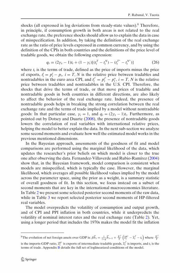
Fig. 3 Impulse response to a preference shock in the euro area

decrease in the euro area more than the reduction of consumption in the U.S.Hence, as noted above, the presence of demand shocks are necessary to explainreal exchange rate dynamics, through their wealth effects on consumption, realwages and relative prices. In our model, these effects are so strong that theyimply a reduction of output as well. Finally, the trade balance deterioratesslightly being consistent with the evidence reported in Monacelli and Perotti(2006). Therefore, it is crucial to have demand shocks in the model, in order tobe able to explain the real exchange rate-relative consumption anomaly.13

Figure 3 shows the impulse response to a preference shock, which hasvery similar effects to the demand shock regarding the implied comovementbetween the real exchange rate and relative consumption. However, unlikethe demand shocks it induces a positive wealth effect generating instead a realexchange rate appreciation. By increasing the marginal utility of consumption,consumption itself increases in the euro area, and the real exchange rate andterms of trade appreciate, which reduces consumption but increases output in

13We also estimate our model assuming non-separable preferences in line with Monacelli andPerotti (2006). Under this specification we were able to reproduce impulse responses conditionalto both fiscal and tradable technology shocks that are consistent with the VAR evidence reportedin Monacelli and Perotti (2006) and Corsetti et al. (2006), respectively. Yet, the likelihooddecreases substantially and the overall fit of this specification underperforms our benchmarkmodel. Results are available upon request from the authors.


-0.10

-0.05

0.00

0.05

0.10

0.15

1985

Q2

1987

Q2

1989

Q2

1991

Q2

1993

Q2

1995

Q2

1997

Q2

1999

Q2

2001

Q2

2003

Q2

Cha

nge

in th

e R

ER

Change in the RER NT Tech

-0.10

-0.05

0.00

0.05

0.10

0.15

1985

Q2

1987

Q2

1989

Q2

1991

Q2

1993

Q2

1995

Q2

1997

Q2

1999

Q2

2001

Q2

2003

Q2

Cha

nge

in th

e R

ER

Change in the RER T. Demand

-0.10

-0.05

0.00

0.05

0.10

0.15

1985

Q2

1987

Q2

1989

Q2

1991

Q2

1993

Q2

1995

Q2

1997

Q2

1999

Q2

2001

Q2

2003

Q2

Cha

nge

in th

e R

ER

Change in the RER Preference

-0.10

-0.05

0.00

0.05

0.10

0.15

1985

Q2

1987

Q2

1989

Q2

1991

Q2

1993

Q2

1995

Q2

1997

Q2

1999

Q2

2001

Q2

2003

Q2

Cha

nge

in th

e R

ER

Change in the RER Other

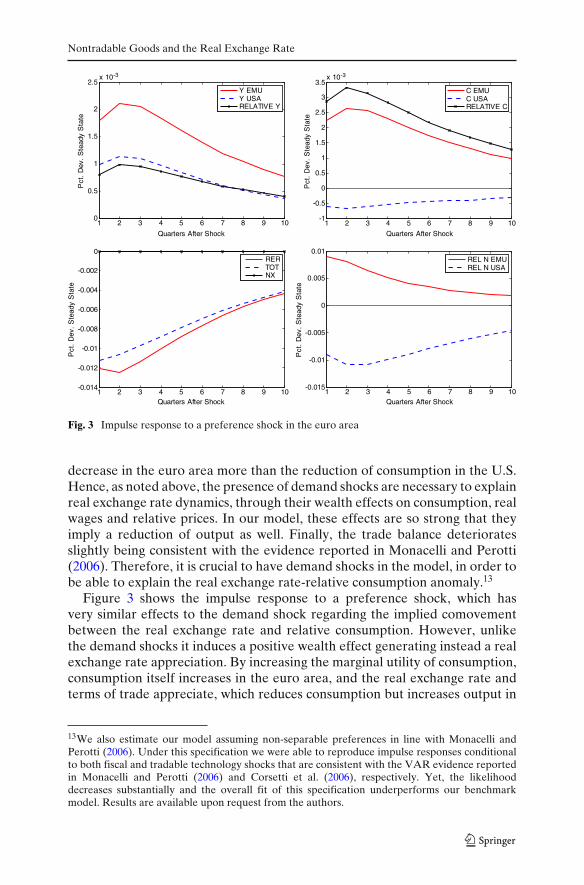
Fig. 4 Decomposition of the real exchange rate

the U.S. due to foreign demand. This also opens a small trade deficit for theeuro area. Why both real exchange and the terms of trade appreciates?. Thepreference shock induces a positive wealth effect that is reflected in higherconsumption. This increase of consumption leads to an increase in wages,marginal cost increases and consequently prices increase in both sectors.The price increase induces both a real exchange rate and terms of tradeappreciation. Again, as noted above, we obtain a negative correlation betweenthe real exchange rate and the ratio of relative consumptions, making thisshock necessary to explain the data. At the same time, the relative price ofnontradables increases in the euro area, but decreases in the U.S.

To further gauge the importance of the previous shocks in accounting for thehistorical RER dynamics, Fig. 4 displays the observed value of the variation inthe real exchange rate (bold line), together with the values with only tradabledemand, nontradable technology, preference, and the other shocks, accordingto our estimated model (dotted lines).14 This exercise allows us to identify thenature of the shocks that have played a dominant role as a source of the realexchange rate dynamics.

It is clear that demand shocks explain a great fraction of the real exchangerate fluctuations being positive correlated with the real exchange rate, resultsthat are consistent with the evidence illustrated above. Hence, the model

14We use the Kalman filter to recover the sequence of shocks. We basically obtain the cyclicalcomponents of the change in the real exchange rate associated with each shock, according to ourestimated model at its posterior mean.


with demand shocks provides a very good approximation to the data. But,as we mentioned before, a model with only demand shocks would imply atoo negative correlation between relative consumptions and the real exchangerate, so this is why other shocks in the model are needed. When the model issimulated with the nontradable component only, we can see that it is also ableto capture some comovement with the actual series. On the other hand, whenthe model is simulated with preference shocks only, or the rest of shocks, thebehavior of the change in the real exchange rate in the model and in the datais quite different.

6 The Role of the Distribution Sector

In recent papers, Corsetti et al. (2008) and Dotsey and Duarte (2008) haveemphasized the role of the distribution sector in explaining real exchangerate dynamics. Here, we follow Dotsey and Duarte (2008) and estimate twodifferent versions of that model. In the first one, we assume that the finaltradable consumption good includes a nontradable intermediate input, and isproduced under monopolistic competition (there is product differentiation). Inthe second case, we further assume that the final tradable good is also pricedwith a Calvo-type restriction.

We modify the model along the following lines. The final tradable goodis consumed by domestic households. This good is produced by a continuumof firms, each producing a differentiated variety, labelled by YT

t (i), i ∈ [0, 1].Each firm combines a composite of home and foreign intermediate tradablegoods XT , with a composite of intermediate nontradable goods X N with thefollowing production function:

YTt (i) =

{γ 1/εY

y

[XT

t (i)] εY −1

εY + (1 − γy)1/εY

[X N

t (i)] εY −1

εY

} εYεY −1

where εy is the elasticity of substitution between tradable and nontradableintermediate goods, and γy is the share of tradable intermediate goods in theproduction function. The nontradable component can be seen as distributionservices needed to bring the final consumption good to consumers. Thisproduction structure somewhat generalizes, but does not nest, Corsetti et al.(2008), and implies a wedge between the price of the CES aggregate of tradableinputs and the price paid by the final consumer, due to distribution costs. Whenγy = 1, we go back to the model of Section 2, but with product differentiationand monopolistic competition in the final tradable goods sector.

The local nontradable intermediate input is a Dixit-Stiglitz aggregate of allnontradable varieties, with the same elasticity than the consumption aggregate:

X Nt (i) ≡

[∫ 1

0X N

t (i, n)σ−1σ dn

] σσ−1


where X Nt (i, n) is the amount of intermediate nontradable input n by final good

producer i. The price level PNt is the same as the one defined in Section 2.

The composite of home and foreign intermediate tradable goods is given by:

XTt (i) =

{γ 1/θ

x

[Xh

t (i)] θ−1

θ + (1 − γx)1/θ[

X ft (i)

] θ−1θ

} θθ−1

The definition of the composite of home and foreign intermediate goodsfollows from Section 2.

Taking a linear approximation to the firm’s optimizing conditions, whenprices of the final tradable good are flexible, delivers the following inflationrate for the final tradable goods sector:

�pTt = γy

[γx�ph

t + (1 − γx) (�p ft + �st)

]+ (1 − γy)�pN

t , (27)

such that the final tradable goods sector includes a nontradable component.Further, if we assume that there are sticky prices in the final tradable goodsector, inflation dynamics in the final goods tradable sector are given by:

�pTt − ϕT�pT

t−1 = βEt(�pT

t+1 − ϕT�pTt

)+ κT(mcT

t − tTt

), (28)

where κT = (1 − αT) (1 − βαT) /αT , mcTt = γy

(tXt + tT

t

)+ (1 − γy)

tNt ,and

tXt = [γx ph

t + (1 − γx) (p ft + st)] − pT

t .Rather than presenting the full set of parameter estimates (which are

available upon request) we compare how the models with a distributionsector fit the data, and in particular some selected moments of the data. InTable 4 we present the marginal likelihoods of the three models (baseline,

Table 4 Model comparison

Data Baseline Distribution Distribution withsticky prices

Marginal likelihood − 3292.2 3222.0 3261.4Standard Deviation(Q/Q−1) 4.64 3.34 3.77 4.34Percent variance explained by

Preference shocks − 23.6 81.1 63.1Nontradable tech. shocks − 31.8 13.5 6.4Fiscal shocks − 43.5 0.8 0.6

Correlation (Q, Q−1) 0.78 0.78 0.75 0.68Correlation (C/C∗, Q) 0.01 0.05 −0.14 −0.23

Note: Standard Deviation(Q/Q−1) is based on raw data, Correlation (Q, Q−1) and Correlation(C/C∗, Q) is based on HP-filtered data


distribution sector with final flexible prices, and distribution sector with finalsticky prices).15

To compare overall performance, we focus on the posterior odds ratiobetween two models A and B:

Pr(model = A| {xt}Tt=1)

Pr( model = B| {xt}Tt=1)

= Pr(A)

Pr(B)

L({xt}Tt=1 |model = A)

L({xt}Tt=1 |model = B)

If one does not have strong views about which model is the true one beforeobserving the data, then Pr(A) = Pr(B), and the researcher updates her beliefson which model is the true one after observing the data according to theBayes factor, which is the ratio of marginal likelihoods between two modelsL({xt}T

t=1|model=A)

L({xt}Tt=1|model=B)

. Introducing a distribution sector in the model does not im-

prove the model fit: a log Bayes factor of 70.2 (=3292.2−3222) implies thatthe researcher would need to have a prior probability that the distributionmodel is the true one about exp(70) times larger than the prior probabilityover the baseline model. When we introduce sticky prices in the final goodssector, model fit improves with respect to the model with flexible goodsprices, but does not reach the value of the baseline model. We conclude thatthe introduction of a distribution sector in the two-sector economy does notimprove its capability of explaining the data, beyond that already included ina two-sector model with tradable and nontradable goods.

Finally, Table 4 includes some additional posterior second moments thatinternational business cycle models would want to replicate. As we can see, theaddition of a distribution sector, and afterwards sticky prices in the final goodstradable sector, increases the volatility of the real exchange rate to valuesthat are closer to those in the data. On the other hand, as we introduce thesefeatures into the models, it becomes more difficult to explain persistence. Anadditional unpleasant result is that, in the models with distribution costs, realexchange rate dynamics end up being explained by preference shocks, whichhave a more difficult interpretation than technology or demand shocks.

7 Concluding Remarks

In this paper we have examined the ability of models with tradable andnontradable goods to fit the data. Our main result is that we are able to match

15The additional parameters γy and the fraction of intermediate goods that is used to produce thefinal tradable good are taken from Dotsey and Duarte (2008). Hence we calibrate γy to 0.62, andthe fraction of nontradable production that is used as an input in the production of final tradedgoods to X N

Y N = 0.4. We also estimated versions of the two distribution cost models where weestimated those parameters. The qualitative results did not change, and model fit did not improvesignificantly. In addition to these two parameters, in the model with a distribution sector andsticky prices, we also estimate αT and ϕT with the same priors than the other Calvo lotteriesand backward looking parameters of Table 1. We also estimate the elasticity of subtitution εy.


real exchange rate persistence, and to less extent, its volatility, with a medium-scale macroeconomic model estimated with Bayesian methods. We have foundthat it is mostly technology shocks in the nontradable sector, and demandshocks in the tradable sector the ones that explain most of the behavior ofthe real exchange rate. When we have estimated versions of the model withdistribution services and sticky prices in the final tradable good sector, we havenot obtained a better model fit. This suggests that distribution costs should notbe treated differently than other nontradables in the production of final goods.

Estimation of DSGE models with several nominal and real rigidities tend toreveal that not all features are necessary to fit the data when priors are not tooinformative (see Galí and Rabanal 2005 or Rabanal and Tuesta 2010). On theother hand, estimated models where priors are much more informative tendto validate the rigidities in place (see Smets and Wouters 2003 and Adolfsonet al. 2007). In our case, we find that distribution services on top of severalother rigidities are not necessary, but this does not mean it is not a featureof relevance in international macroeconomics, or to explain the apparentdeviation from the law of one price in industry-level data. In any case, we havefound that a two-sector two-country model in the spirit of Stockman and Tesar(1995), complemented with nominal rigidities and habit formation, seems todo a good job in explaining the data.

Appendix A: The Baseline Model

In this appendix, we present the full version of a model with tradable andnontradable final consumption goods, in the spirit of Stockman and Tesar(1995) and Dotsey and Duarte (2008). We introduce sticky prices in bothsectors to be able to study inflation dynamics and their role in affecting thereal exchange rate.

A.1 Households

A.1.1 Preferences

Representative households in the home country are assumed to maximize thefollowing utility function:

Ut = E0

{ ∞∑t=0

β tψt

[log(Ct − bCt−1

)− L1+ϕt

1 + ϕ

]}, (29)

subject to the following budget constraint:

BHt

Pt Rt+ St BF

t

Pt R∗t �(

St BFt

PtYt

) ≤ BHt−1

Pt+ St BF

t−1

Pt+ Wt

PtLt − Ct + �t (30)

E0 denotes the conditional expectation on information available at date t = 0,

β is the intertemporal discount factor, with 0 < β < 1. Ct denotes the level of


consumption in period t, Lt denotes labor supply. The utility function displaysexternal habit formation with respect to the habit stock, which is last period’saggregate consumption of the economy Ct−1. b ∈ [0, 1] denotes the importanceof the habit stock. ϕ > 0 is inverse elasticity of labor supply with respect to thereal wage. ψt is a preference shock that follows an AR(1) process in logs

log ψt = ρψ log ψt−1 + εψt (31)

We define the consumption index as

Ct ≡[γ 1/ε

c

(CT

t

) ε−1ε + (1 − γc)

1/ε(CN

t

) ε−1ε

] εε−1

,

where ε is elasticity of substitution between the final tradable (CTt ) and final

nontradable (CNt ) goods, and γc is the share of final tradable goods in the

consumption basket at home.In this context, the consumer price index that corresponds to the previous

specification is given by

Pt ≡[γc(PT

t

)1−ε + (1 − γc)(PN

t

)1−ε] 1

1−ε

,

where all prices are for goods sold in the home country, in home currency andat consumer level, for both tradable and nontradable goods.

Demands for the final tradable and nontradable goods are given by:

CTt = γc

(PT

t

Pt

)−ε

Ct,

CNt = (1 − γc)

(PN

t

Pt

)−ε

Ct.

A.1.2 Incomplete Asset Markets

For modelling simplicity, we choose to model incomplete markets with tworisk-free one-period nominal bonds denominated in domestic and foreigncurrency, and a cost of bond holdings is introduced to achieve stationarity.Then, the budget constraint of the domestic households in real units of homecurrency is given by:

BHt

Pt Rt+ St BF

t

Pt R∗t �(

St BFt

PtYt

) ≤ BHt−1

Pt+ St BF

t−1

Pt+ Wt

PtLt − Ct + �t (32)

where Wt is the nominal wage, and �t are real profits for the home consumer.BH

t is the holding of the risk free domestic nominal bond and BFt is the holding

of the foreign risk-free nominal bond expressed in foreign country currency.St is the nominal exchange rate, expressed in units of home country currencyper unit of foreign country. The function �(.) depends on the net liabilityposition (i.e. the negative net foreign asset position) of the home country,BF

t , in percent of GDP in the entire economy, and is taken as given by the


domestic household.16 �(.) introduces a convex cost that allows to obtain awell-defined steady state, and captures the costs of undertaking positions inthe international asset market.17

A.2 Production Sector

The production of this economy is undertaken by three sectors. First, there is afinal goods sector, that uses intermediate tradable inputs from both countriesand operates under perfect competition, to produce the final tradable goods.This same sector also aggregates varieties of the nontradable goods to producea final nontradable good that is sold to households. The second sector producesintermediate tradable goods, which are used as an input for the productionof final goods both in the home and in the foreign country. The third sectorproduces nontradable goods, that are used as inputs in the production of thefinal nontradable good.

A.2.1 Final Goods Sector

The final tradable good is consumed by domestic households. This good isproduced by a continuum of firms, each producing the same variety, labelled by

YTt , using intermediate home

(Xh

t

)and foreign

(X f

t

)goods with the following

technology:

YTt =

{γ 1/θ

x

(Xh

t

) θ−1θ + (1 − γx)

1/θ(

X ft

) θ−1θ

} θθ−1

where θ is the elasticity of substitution between home-produced and foreign-produced imported intermediate goods, and γx is the share of home goodsin the production function. We further assume symmetric home-bias in thecomposite of intermediate tradable goods. The corresponding composite ofhome and foreign intermediate tradable goods abroad is given by

YT∗t =

{(1 − γx)

1/θ(Xh∗

t

) θ−1θ + γ 1/θ

x

(X f ∗

t

) θ−1θ

} θθ−1

Xht and X f

t , that denote the amount of home and foreign intermediate tradableinputs to produce the final tradable good at home, are also Dixit-Stiglitz

16As Benigno (2009) points it out, some restrictions on φ (.) are necessary: φ (0) = 1; assumes thevalue 1 only if BF,t = 0; differentiable; and decreasing in the neighborhood of zero.17Another way to describe this cost is to assume the existence of intermediaries in the foreign assetmarket (which are owned by the foreign households) who can borrow and lend to households ofcountry F at a rate (1 + r∗), but can borrow from and lend to households of country H at a rate(1 + r∗)φ (.).


aggregates of all types of home and foreign final goods, with elasticity ofsubstitution σ :

Xht ≡

[∫ 1

0Xh

t (h)σ−1σ dh

] σσ−1

and

X ft ≡

[∫ 1

0X f

t ( f )σ−1σ df

] σσ−1

where Xht (h) and X f

t ( f ) denote individual quantities from intermediate trad-able goods producers at home and foreign. The equivalent quantities forforeign final tradable goods producers are Xh∗

t (h) and X f ∗t ( f ). Optimizing

conditions by final tradable goods producers deliver the following demandfunctions:

Xht (h) = γx

(Ph

t (h)

Pht

)−σ (Ph

t

PTt

)−θ

YTt ;

Xh∗t (h) = (1 − γx)

(Ph∗

t (h)

Ph∗t

)−σ (Ph∗

t

PT∗t

)−θ

YT∗t

X ft ( f ) = (1 − γx)

(P f

t ( f )

P ft

)−σ (P f

t

PTt

)−θ

YTt ;

X f ∗t ( f ) = γx

(P f ∗

t ( f )

P f ∗t

)−σ (P f ∗

t

PT∗t

)−θ

YT∗t

where

Pht ≡

[∫ 1

0Ph

t (h)1−σ dh] 1

1−σ

, P ft ≡

[∫ 1

0P f

t ( f )1−σ df] 1

1−σ

.

and

PTt =

[γx(Ph

t

)1−θ + (1 − γx)(

P ft

)1−θ] 1

1−θ

We assume that the law of one price holds for intermediate inputs, such thatPh

t (h) = Ph∗t (h)St, and P f

t ( f ) = P f ∗t ( f )St, where St is the nominal exchange

rate.The production of the final nontradable good is given by:

Y Nt ≡

[∫ 1

0X N

t (n)σ−1σ dn

] σσ−1


where we assume the same elasticity σ > 1 than in the case of final tradablegoods produced within country H. The price level for nontradables is

PNt ≡

[∫ 1

0pN

t (n)1−σ dn] 1

1−σ

A.2.2 Intermediate Non-Tradable Goods Sector

The intermediate nontradable sector produces differentiated goods that areaggregated by final good producing firms, and ultimately used for finalconsumption by domestic households only. Each firm produces intermediatenontradable goods according to the following production function

Y Nt (n) = At Z N

t LNt (n) (33)

where At is a labor augmenting aggregate world technology shock which has aunit root with drift, as in Galí and Rabanal (2005):

log At = g + log At−1 + εat (34)

This shock also affects the intermediate tradable sector production function.Hence, real variables in both countries grow at a rate g. Z N

t is the country-specific productivity shock to the nontradable sector at time t which evolvesaccording to an AR(1) process in logs

log Z Nt = (1 − ρN) log(Z N) + ρZ ,N log Z N

t−1 + εZ ,Nt (35)

Firms in the nontradable sector face a Calvo lottery when setting their prices.Each period, with probability 1 − αN , firms receive a stochastic signal that al-lows them to reset prices optimally. We assume that there is partial indexationwith a coefficient ϕN to last period’s sectorial inflation rate for those firms thatdo not get to reset prices. As a result, firms maximize the following profitsfunction:

MaxPNt (n)Et

∞∑k=0

αkN�t,t+k

⎧⎪⎨⎪⎩⎡⎢⎣ PN

t (n)(

PNt+k−1

PNt−1

)ϕN

Pt+k− MCN

t+k

⎤⎥⎦Y N,d

t+k (n)

⎫⎪⎬⎪⎭ (36)

subject to

Y N,dt+k (n) =

[(PN

t (n)

PNt+k

)(PN

t+k−1

PNt−1

)ϕN]−σ

Y Nt (37)

where Y N,dt (n) is total individual demand for a given type of nontradable

good n, and Y Nt is aggregate demand for nontradable goods, as defined above.

�t,t+k = βk λt+kλt

is the stochastic discount factor, where λt = ψtCt−bCt−1

is themarginal utility of consumption. MCN

t corresponds to the real marginal costin the nontradable sector. From cost minimization:

MCNt = Wt

Pt Z Nt At


A.2.3 Intermediate Tradable Goods Sector

The intermediate tradable sector produces differentiated goods that are soldto the final sector goods producers in the home and foreign countries. Mostfunctional forms are similar to those presented for the nontradable sector.

Each firm produces tradable intermediate goods according to the followingproduction function

Yht (h) = At Z h

t Lht (h) (38)

where Z ht is the country-specific productivity shock to the intermediate goods

tradable sector at time t which evolves according to an AR(1) process in logs

log Z ht = (1 − ρh) log(Z h) + ρZ ,h log Z h

t−1 + εZ ,ht (39)

Firms in the intermediate tradable sector face the same Calvo lottery as firmsin the intermediate nontradable sector, with relevant parameters αh and ϕh:

MaxPht (h)Et

∞∑k=0

αkh�t,t+k

⎧⎪⎨⎪⎩⎡⎢⎣ Ph

t (h)(

Pht+k−1

Pht−1

)ϕh

Pt+k− MCh

t+k

⎤⎥⎦Yh,d

t+k (h)

⎫⎪⎬⎪⎭ (40)

subject to

Yh,dt+k (h) = Xh

t+k(h) + Xh∗t+k(h)

=[(

Pht (h)

Pht+k

)(Ph

t+k−1

Pht−1

)ϕh]−σ

Xht (41)

where Yh,dt (h) is total individual demand for a given type of tradable interme-

diate good h, and Xht is aggregate demand for intermediate good h, consisting

of home demand, and foreign demand:

Xht =

[γx

(Ph

t

PTt

)−θ

YTt + (1 − γx)

(Ph∗

t

PT∗t

)−θ

YT∗t

]

MCht corresponds to the real marginal cost in the nontradable sector. From

cost minimization:

MCht = Wt

Pt Z ht At

A.2.4 Market Clearing

We assume that the demand shock is allocated between tradable and non-tradable goods in the same way that private consumption is. Hence the


market clearing conditions for both types of final goods, consisting of privateconsumption and the demand shock in the tradadable sector, are:

YTt = CT

t + GTt

Y Nt = CN

t + GNt

where GNt , GT

t follow AR(1) processes in logs. The bond market clearingconditions are

BHt + BH∗

t = 0 (42)

BFt + BF∗

t = 0 (43)

For the nontradable intermediate goods, the market clearing condition is:

Y Nt (n) = X N

t , for all n ∈ [0, 1] (44)

while for the intermediate tradable goods sector it is:

Yht (h) = Xh

t (h) + Xh∗t (h), for all h ∈ [0, 1] (45)

For the labor market:

Lt = Lht + LN

t = (46)

=∫ 1

0Lh

t (h)dh +∫ 1

0LN

t (n)dn

A.3 Optimizing, Market Clearing Conditions, and Monetary Policy

In this subsection we present the full set of equations characterizing thesymmetric equilibrium. Since all agents in each economy are equal, then theper capita and aggregate consumption levels are equal (Ct = Ct), as well as thenet foreign assets levels (BF

t = BFt ).

A.3.1 Households

The Euler equations for home and foreign households, and the optimalcondition of holdings by home household of the foreign bond are:

λt = βEt

{Rt

Pt

Pt+1λt+1

}

λ∗t = βEt

{R∗

tP∗

t

P∗t+1

λ∗t+1

}

λt = �

(St BF

t

PtYt

)βEt

{R∗

tQt+1

Qtλt+1

}


where λt is the marginal utility of consumption:

λt = UC (Ct) = ψt

Ct − bCt−1

λ∗t = UC

(C∗

t

) = ψ∗t

C∗t − b ∗C∗

t−1

The labor supply decisions in each country are:

λtWt

Pt= Lϕ

t

λ∗t

W∗t

P∗t

= (L∗t

)ϕ∗

where:

Lt = Lht + LN

t

and

L∗t = Lh∗

t + LN∗t

Household demand for final tradable and nontradable goods are given by:

CTt = γc

(PT

t

Pt

)−ε

Ct,

CNt = (1 − γc)

(PN

t

Pt

)−ε

Ct.

CT∗t = γ ∗

c

(PT∗

t

P∗t

)−ε∗

C∗t ,

CN∗t = (1 − γ ∗

c )

(PN∗

t

P∗t

)−ε

C∗t

and the CPI’s in each country are given by:

Pt ≡[γc(PT

t

)1−ε + (1 − γc)(PN

t

)1−ε] 1

1−ε

,

P∗t ≡

[γ ∗

c

(PT∗

t

)1−ε + (1 − γ ∗c )(PN∗

t

)1−ε] 1

1−ε

The real exchange rate is

Qt = St P∗t

Pt


A.3.2 Final Goods Producers

The production of final tradable goods in both countries is given by:

YTt =

{γ 1/θ

x

(Xh

t

) θ−1θ + (1 − γx)

1/θ(

X ft

) θ−1θ

} θθ−1

and

YT∗t =

{(1 − γx)

1/θ(Xh∗

t

) θ−1θ + γ 1/θ

x

(X f ∗

t

) θ−1θ

} θθ−1

Demand for intermediate tradable goods is:

Xht = γx

(Ph

t

PTt

)−θ

YTt ; Xh∗

t = (1 − γx)

(Ph∗

t

PT∗t

)−θ

YT∗t

X ft = (1 − γx)

(P f

t

PTt

)−θ

YTt ; X f ∗

t ( f ) = γx

(P f ∗

t

PT∗t

)−θ

YT∗t

where

Pht ≡

[∫ 1

0Ph

t (h)1−σ dh] 1

1−σ

, P ft ≡

[∫ 1

0P f

t ( f )1−σ df] 1

1−σ

.

The price of final tradable goods is:

PTt =

[γx(Ph

t

)1−θ + (1 − γx)(

P ft

)1−θ] 1

1−θ

and

PT∗t =

[γ ∗

x

(Ph∗

t

)1−θ + (1 − γ ∗x )(

P f ∗t

)1−θ] 1

1−θ

Since we assumed that the law of one price holds for intermediate goods, italso holds in the aggregate, such that Ph

t = Ph∗t St, and P f

t = P f ∗t St, where St is

the nominal exchange rate.

A.3.3 Nontradable Goods Producers

The price setting equations are given by the following optimal expressions:

pNt

PNt

= σ

(σ − 1)Et

⎧⎪⎪⎪⎪⎪⎪⎨⎪⎪⎪⎪⎪⎪⎩

∞∑k=0

βkαkNλt+k

(k∏

s=1

(�N

t+s−1

)ϕN

�Nt+s

)−σ

MCNt+kY N

t+k

∞∑k=0

βkαkNλt+k

(k∏

s=1

(�N

t+s−1

)ϕN

�Nt+s

)1−σ

PNt+k

Pt+kY N

t+k

⎫⎪⎪⎪⎪⎪⎪⎬⎪⎪⎪⎪⎪⎪⎭


where

MCNt = Wt

Pt Z Nt At

,

Y Nt = CN

t + GNt


PNt ≡

[αN

(PN

t−1

(�N

t−1

)ϕN)1−σ + (1 − αN)

(pN

t

)1−σ] 1

1−σ

where �Nt−1 = PN

t−1

PNt−2

.

The production function is:

Y Nt = At Z N

t LNt .

In the foreign country these expressions are:

pN∗t

PN∗t

= σ

(σ − 1)Et

⎧⎪⎪⎪⎪⎪⎪⎨⎪⎪⎪⎪⎪⎪⎩

∞∑k=0

βkαkN∗λt+k

(k∏

s=1

(�N∗

t+s−1

)ϕN∗

�N∗t+s

)−σ

MCN∗t+kY N∗

t+k

∞∑k=0

βkαkN∗λt+k

(k∏

s=1

(�N∗

t+s−1

)ϕN∗

�N∗t+s

)1−σ

PN∗t+k

Pt+kY N∗

t+k

⎫⎪⎪⎪⎪⎪⎪⎬⎪⎪⎪⎪⎪⎪⎭

where

MCN∗t = Wt

Pt Z N∗t At

,

Y N∗t = CN∗

t + GN∗t


PN∗t ≡

[αN∗

(PN∗

t−1

(�N∗

t−1

)ϕN∗)1−σ + (1 − αN∗)(

pN∗t

)1−σ] 1

1−σ

where �N∗t−1 = PN∗

t−1

PN∗t−2

.


Y N∗t = At Z N∗

t LN∗t .

A.3.4 Intermediate Traded Goods Producers

The price setting equations are given by the following optimal expressions:

pht

Pht

= σ

(σ − 1)Et

⎧⎪⎪⎪⎪⎪⎪⎨⎪⎪⎪⎪⎪⎪⎩

∞∑k=0

βkαkhλt+k

(k∏

s=1

(�h

t+s−1

)ϕh

�ht+s

)−σ

MCht+kYh

t+k

∞∑k=0

βkαkhλt+k

(k∏

s=1

(�h

t+s−1

)ϕh

�ht+s

)1−σ

Pht+k

Pt+kYh

t+k

⎫⎪⎪⎪⎪⎪⎪⎬⎪⎪⎪⎪⎪⎪⎭


where

MCht = Wt

Pt Z ht At

,

Yht = Xh

t + Xh∗t .

The evolution of the price level of final tradables is

Pht ≡

[αh

(Ph

t−1

(�h

t−1

)ϕh)1−σ + (1 − αh)

(ph

t

)1−σ] 1

1−σ

where �ht−1 = Ph

t−1

Pht−2

.


Yht = At Z h

t Lht

In the foreign country, this expressions are:

p f ∗t

P f ∗t

= σ

(σ − 1)Et

⎧⎪⎪⎪⎪⎪⎪⎪⎪⎪⎨⎪⎪⎪⎪⎪⎪⎪⎪⎪⎩

∞∑k=0

βkαkf ∗λt+k

⎛⎜⎝ k∏

s=1

(�

f ∗t+s−1

)ϕ f∗

�f ∗t+s

⎞⎟⎠

−σ

MC f ∗t+kY f ∗

t+k

∞∑k=0

βkαkf ∗λt+k

⎛⎜⎝ k∏

s=1

(�

f ∗t+s−1

)ϕ f∗

�f ∗t+s

⎞⎟⎠

1−σ

P f ∗t+k

Pt+kY f ∗

t+k

⎫⎪⎪⎪⎪⎪⎪⎪⎪⎪⎬⎪⎪⎪⎪⎪⎪⎪⎪⎪⎭

where

MC f ∗t = Wt

Pt Zf ∗

t At

,

Y f ∗t = X f

t + X f ∗t .

The evolution of the price level of final tradables is

P f ∗t ≡

[α f ∗(

P f ∗t−1

(�

f ∗t−1

)ϕ f∗)1−σ + (1 − α f ∗)(

p f ∗t

)1−σ] 1

1−σ

where �f ∗t−1 = P f∗

t−1

P f∗t−2

.


Y f ∗t = At Z

f ∗t L f ∗

t


A.3.5 Monetary Policy

Monetary policy in both countries is conducted with a Taylor rule that targetsCPI inflation and output growth deviation from steady-state values:

Rt = R(1−ρr) Rρrt−1

(Pt/Pt−1

�

)(1−ρr)γπ(

Yt/Yt−1

1 + g

)(1−ρr)γy

exp(εrt )

R∗t = R∗(1−ρ∗

r )(R∗

t−1

)ρ∗r

(P∗

t /P∗t−1

�∗

)(1−ρ∗r )γ ∗

π(

Y∗t /Y∗

t−1

1 + g

)(1−ρ∗r )γ ∗

y

exp(εr∗t )

A.3.6 Demand Shocks

GTt = (GT)(1−ρGT )(GT

t−1)ρGT exp(εGT

t )

GNt = (GN)(1−ρGN )(GN

t−1)ρGN exp(εGN

t )

GT∗t = (GT∗

)(1−ρGT∗ )(GT∗t−1)

ρGT∗ exp(εGT∗t )

GN∗t = (GN∗

)(1−ρGN∗ )(GN∗t−1)

ρGN∗ exp(εGN∗t )

A.3.7 Trade Balance and Net Foreign Asset Dynamics

We present the evolution of the trade balance and net foreign assets of thehome country, since the definition those in the foreign country will mirrorthose in the home country. Holdings of foreign bonds depend on the tradebalance (NXt) as follows

St BFt

Pt R∗t �(

St BFt

PtYt

) = St BFt−1

Pt+ NXt

Since international trade only occurs at the intermediate goods level, netexports equal exports minus imports of intermediate goods:

NXt = Pht Xh∗

t − P ft X f

t

Pt

Finally, we define nominal GDP to be equal to aggregate nominal private andpublic consumption, hence PtYt = PT

t (CTt + GT

t ) + PNt (CN

t + GNt ).


Appendix B: Log-Linear Version of the Model

Euler equations

b�ct = − (1 + g − b) (rt − Et�pt+1) + (1 + g) Et�ct+1

+ (1 + g − b)(1 − ρψ

)ψt (47)

b ∗�c∗t = − (1 + g − b ∗) (r∗

t − Et�p∗t+1

)+ (1 + g) Et�c∗t+1

+ (1 + g − b ∗) (1 − ρ∗ψ

)ψ∗

t (48)

Risk sharing

Et (qt+1 − qt) =[(1 + g) Et�ct+1 − b�ct

(1 + g − b)

]−[(1 + g) Et�c∗

t+1 − b ∗�c∗t

(1 + g − b ∗)

]

+ (1 − ρψ

)ψt − (1 − ρ∗

ψ

)ψ∗

t + χb t (49)

where χ ≡ −�′ (0) Y, b t =(

St BFt

Pt

)Y−1.

The labor supply schedules are given by:

ωt = ϕlt +[

1 + g1 + g − b

]ct − b

(1 + g − b)ct−1 + b

(1 + g − b)εa

t (50)

ω∗t = ϕl∗t +

[1 + g

1 + g − b ∗

]c∗

t − b ∗

(1 + g − b ∗)c∗

t−1 + b ∗

(1 + g − b ∗)εa

t (51)

Technology

yht = lh

t + zht − εa

t (52)

yh∗t = lh∗

t + zh∗t − εa

t (53)

yNt = lN

t + zNt − εa

t (54)

yN∗t = lN∗

t + zN∗t − εa

t (55)

Consumer price inflation

�pt = γc�pTt + (1 − γc) �pN

t (56)

�pt = γc∗�pT∗t + (1 − γc∗)�pN∗

t (57)

Tradable inflation

�pTt = γx�ph

t + (1 − γx) (�p f ∗t + �st) (58)

�pT∗t = γx∗(�ph

t − �st) + (1 − γx∗) �p f ∗t (59)


Price setting in the nontradable sector

�pNt − ϕN�pN

t−1 = βEt(�pN

t+1 − ϕN�pNt

)+ κN(wt − zN

t − tNt

)(60)

�pN∗t − ϕN∗�pN∗

t−1 = βEt(�pN∗

t+1 − ϕ∗N�pN∗

t

)+ κN∗(w∗

t − zN∗t − tN∗

t

)(61)

where κN = (1 − αN) (1 − βαN) /αN, κN∗ = (1 − αN∗) (1 − βαN∗) /αN∗ , tN =pN

t − pt, and tN∗ = pN∗t − pt.

Price setting in the intermediate tradable good sector

�pht − ϕh�ph

t−1 = βEt(�ph

t+1 − ϕh�pht

)+ κh(wt − zh

t − tht − tT

t

)(62)

�p f ∗t − ϕ f ∗�p f ∗

t−1 = βEt

(�p f ∗

t+1 − ϕ∗f �p f ∗

t

)+ κ f ∗

(w∗

t − z f ∗t − t f ∗

t − tT∗t

)(63)

where κh = (1 − αh) (1 − βαh) /αh, κ f ∗ = (1 − α f ∗) (

1 − βα f ∗)/α f ∗ , th

t = pht −

pTt , t f ∗

t = p f ∗t − pT∗

t , tT = pTt − pt, and tT∗ = pT∗

t − pt.Final consumption demand

cTt = −εtT

t + ct (64)

cT∗t = −ε∗tT∗

t + c∗t (65)

cNt = −εtN

t + ct (66)

cN∗t = −ε∗tN∗

t + c∗t (67)

Intermediate tradable and nontradable demand

xht = −θ th

t + yTt (68)

xh∗t = −θ th∗

t + yT∗t (69)

x ft = −θ t f

t + yTt (70)

x f ∗t = −θ t f ∗

t + yT∗t (71)

Relative Price IndexLet’s define tt = p f

t

pht, since the law of one price holds tt = −t∗t = ph∗

t

p f∗t

, then we

can write the following relative prices as a function of tt.

tht = − (1 − γx) tt (72)

th∗t = −γxtt (73)

t ft = γxtt (74)

t f ∗t = (1 − γx) tt (75)


Relative prices

tt = tt−1 + �st + �p f ∗t − �ph

t (76)

tTt = tT

t−1 + �pTt − �pt (77)

tNt = − γc

1 − γctTt (78)

tT∗t = tT∗

t−1 + �pT∗t − �p∗

t (79)

tN∗t = − γ ∗

c

1 − γ ∗c

tT∗t (80)

qt = qt−1 + �st + �p∗t − �pt (81)

Taylor rules

rt = ρrrt−1 + (1 − ρr) γπ�pt + γy�yt + εrt (82)

r∗t = ρ∗

r r∗t−1 + (1 − ρr∗) γ ∗

π �p∗t + γ ∗

y �yt + εr∗t (83)

Net foreign assets and net exports

βb t − 11 + g

b t−1 = nxt (84)

nxt = X f

Y

(xh∗

t − x ft − tt

)(85)

where b t = BFt St

PtYis the debt to GDP ratio, and nxt = NXt

Y , and where we haveassumed balanced trade in the steady state. To solve for the steady-state ratios,we have that:

YT

Y= GT

G= CT

C= γc

Y N

Y= GN

G= CN

C= 1 − γc

Xh

YT= γx,

X f

YT= 1 − γx

Therefore tradable GDP over total GDP is

Xh

Y= Xh

YT

YT

Y= γxγc.


Hence

X f

Y= X f

XT

XT

YT

YT

Y= (1 − γx)γc.

Market clearing:

yTt = (1 − γ )cT

t + γ gTt (86)

where γ equals the fraction of government spending over total output. For thenontradable good, the market clearing condition is:

yNt = (1 − γ )cN

t + γ gNt (87)

Finally, for the intermediate tradable goods sector:

yht = γxxh

t + (1 − γx) xh∗t (88)

Total real GDP

yt = γc(tTt + yT

t ) + (1 − γc) (tNt + yN

t ) (89)

total labor

lt = Xh

Xh + Y Nlht + Y N

Xh + Y NlNt (90)

For the foreign country:

yT∗t = (1 − γ ∗)cT∗

t + γ ∗gT∗t (91)

yN∗t = (1 − γ ∗)cN∗

t + γ ∗gN∗t (92)

y f ∗t = γ ∗

x x f ∗t + (1 − γ ∗

x

)x f

t (93)

y∗t = γ ∗

c (tT∗t + yT∗

t ) + (1 − γ ∗c

)(tN∗

t + yN∗t ) (94)

lt = Y f ∗

Yh + Y Nl f ∗t + Y N∗

Y f ∗ + Y N∗ lN∗t (95)

Mapping variables in the model with observable variables.

ct − ct−1 = �ct − εat (96)

c∗t − c∗

t−1 = �c∗t − εa

t (97)

yt − yt−1 = �yt − εat (98)

y∗t − y∗

t−1 = �y∗t − εa

t (99)


Shocks

ψt = ρψψt−1 + εψt

ψ∗t = ρψ∗ψ∗

t−1 + εψ∗t

zht = ρZ ,hzh

t−1 + εZ ,ht

z f ∗t = ρZ , f ∗

z f ∗t−1 + ε

Z , f ∗t

zNt = ρZ ,NzN

t−1 + εZ ,Nt

zN∗t = ρZ ,N∗

zN∗t−1 + ε

Z ,N∗t

gTt = ρG,T gT

t−1 + εG,Tt

gNt = ρG,NgN

t−1 + εG,Nt

gT∗t = ρG,T∗

gT∗t−1 + ε

G,T∗t

gN∗t = ρG,N∗

gN∗t−1 + ε

G,N∗t

and εat , ε

rt , ε

r∗t are iid shocks.

References

Adolfson M, Laseen S , Lindé J, Villani M (2007) Bayesian estimation of an open economy dsgemodel with incomplete pass-through. J Int Econ 72(2):481–511

An S, Schorfheide F (2007) Bayesian analysis of DSGE models. Econom Rev 26(2–4):113–172Betts C, Kehoe T (2006) U.S. real exchange rate fluctuations and relative price fluctuations.

J Monet Econ 53:1297–1326Benigno P (2009) Price stability with imperfect financial integration. Journal of Money, Credit and

Banking, vol 41(s1). Blackwell Publishing, pp 121–149Benigno G, Thoenissen C (2008) Consumption and real exchange rates with incomplete markets

and non-traded goods. J Int Money Financ 27:926–948Clarida R, Galí J, Gertler M (2000) Monetary policy rules and macroeconomic stability: evidence

and some theory. Q J Econ 115:147–180Chari VV, Kehoe P, McGrattan E (2002) Can sticky price models generate volatile and persistent

real exchange rates? Rev Econ Stud 69:533–563Corsetti G, Dedola L, Leduc S (2008) International risk sharing and the transmission of produc-

tivity shocks. Rev Econ Stud 75(2):443–473Corsetti G, Dedola L, Leduc S (2006) Productivity, external balance and exchange rates: evidence

on the transmission mechanism among G7 countries. Prepared for the 2006 NBER interna-tional seminar on macroeconomics

Debaere P, Lee H (2004) The real-side determinants of countries´ terms of trade: a panel dataanalysis, mimeo. University of Texas, Austin

De Walque G, Smets F, Wouters R (2005) An open economy dsge model linking the euro areaand the US economy. Manuscript, National Bank of Belgium and European Central Bank

Dotsey M, Duarte M (2008) Nontradable goods, market segmentation, and exchange rates.J Monet Econ 55(6):1129–1142


Engel C (1999) Accounting for U.S. Real Exchange Rate Changes. Journal of Political Economy,vol 107(3). University of Chicago Press, pp 507–538

Fernández-Villaverde J, Rubio-Ramírez JF (2004) Comparing dynamic equilibrium models todata: a Bayesian approach. J Econ 123:153–187

Galí J, Rabanal P (2005) Technology shocks and aggregate fluctuations: how well does the realbusiness cycle model fit postwar U.S. data?, NBER Chapters. In: NBER macroeconomicsannual 2004, vol 19. National Bureau of Economic Research, Inc., pp 225–318

Ireland P (2006) Changes in the federal reserve’s inflation target: causes and consequences.Mimeo, Boston College

Justiniano A, Preston B (2010) Can structural small open economy models account for theinfluence of foreign disturbances? J Int Econ Elsevier 81(1):61–74

Lubik T, Schorfheide F (2005) A Bayesian look at new open economy macroeconomics, NBERMacroeconomics Annual 2005, pp 313–366

Mandelman F, Rabanal P, Rubio-Ramirez JF, Vilán D (2011) Investment-specific technologyshocks and international business cycles: an empirical assessment. Rev Econ Dyn 14(1):136–155

Monacelli T, Perotti R (2006) Fiscal policy, the trade balance, and the real exchange rate: implica-tions for international risk sharing. Mimeo, Universitá Bocconi

Rabanal P, Rubio-Ramírez JF (2005) Comparing new keynesian models of the business cycle: aBayesian approach. J Monet Econ 52(6):1151–1166

Rabanal P, Rubio-Ramírez JF (2008) Comparing new keynesian models in the euro area: aBayesian approach. Span Econ Rev 10:23–40

Rabanal P, Tuesta V (2010) Euro-dollar real exchange rate dynamics in an estimated two-countrymodel: an assessment. J Econ Dyn Control 34:780–797

Rogoff K (1996) The purchasing power parity puzzle. J Econ Lit 4:647–68Schmitt-Grohe S, Uribe M (2011) Business cycles with a common trend in neutral and investment-

specific productivity. Rev Econ Dyn 14(1):122–135Smets F, Wouters R (2003) An estimated dynamic stochastic general equilibrium model of the

euro area. Journal of the European Economic Association, vol 1(5). MIT Press, pp 1123–1175Steinsson J (2008) The dynamic behavior of the real exchange rate in sticky price models.

Am Econ Rev 98:519–533Stockman AC, Tesar LL (1995) Tastes and technology in a two-country model of the business

cycle: explaining international comovements. Am Econ Rev 85(1):168–185

Nontradable Goods and the Real Exchange Rate · Nontradable Goods and the Real Exchange Rate...

Documents

Transcript of Nontradable Goods and the Real Exchange Rate · Nontradable Goods and the Real Exchange Rate...