Nonstandard discretizations of the generalized Nagumo reaction-diffusion equation

Nonstandard Discretizations of the GeneralizedNagumo Reaction-Diffusion EquationZ. Chen,1 A. B. Gumel,1 R. E. Mickens2

1 Department of Mathematics, University of Manitoba, Winnipeg, Manitoba,R3T 2N2, Canada

2 Department of Physics, Clark Atlanta University, Atlanta, Georgia 30314

Received 3 April 2002; accepted 8 July 2002

DOI 10.1002/num.10048

A competitive nonstandard semi-explicit finite-difference method is constructed and used to obtainnumerical solutions of the diffusion-free generalized Nagumo equation. Qualitative stability analysis andnumerical simulations show that this scheme is more robust in comparison to some standard explicitmethods such as forward Euler and the fourth-order Runge-Kutta method (RK4). The nonstandard schemeis extended to construct a semi-explicit and an implicit scheme to solve the full Nagumo reaction-diffusionequation. © 2003 Wiley Periodicals, Inc. Numer Methods Partial Differential Eq 19: 363–379, 2003

Keywords: nonstandard finite-difference schemes; truncation errors; convergence; Nagumo model; pos-itivity

1. INTRODUCTION

Reaction-diffusion equations are known to feature in the mathematical modeling of manyreal-life phenomena such as celestial mechanics, electric impulses along nerve axons, popula-tion biology, etc. [1–5]. For example, the well-known Nagumo reaction-diffusion equation,which has applications in nerve conduction, is given by

�u

�t� u�u � a��1 � u� �

�2u

�x2 , (1)

where u � u(x, t) and a � 0 is a parameter. We consider a generalized version of (1) involvingcontrol parameters �, � and diffusion coefficient D, given by

Correspondence to: A. B. Gumel, Department of Mathematics, 342 Manchray Hall, University of Manitoba, Winnipeg,Manitoba, Canada R3T 2N2 (e-mail: [email protected])Contract grant sponsors: NSERC of Canada (ABG), DOE (REM), and the MBRS-SCORE Program at Clark AtlantaUniversity.

© 2003 Wiley Periodicals, Inc.

�u

�t� D

�2u

�x2 � �u � �u3. (2)

The aim of this study is to, first of all, construct, and analyze, a robust numerical method forthe solution of the diffusion-free Nagumo equation. This method, which will be seen to bequalitatively equivalent to the corresponding continuous model for realistic initial and parametervalues, will then be extended to solve the full Nagumo reaction-diffusion equation.

It is well known that using standard numerical integration techniques, such as the explicitEuler and Runge-Kutta (RK) methods, to solve initial-value problems often leads to contrivednumerical instabilities for certain choices of model and discretization parameters [2–4, 6–8].Although such instabilities, which include contrived oscillations and chaos, can generally beremoved by using small time steps (such as by using numerical integrators which employadaptive step size), the extra computing cost associated with examining the long-term behaviorof a dynamical system can be substantial. Thus, it is desirable to design robust numericalmethods that not only admit large time-steps, but are also free of scheme-dependent instabilitiesfor realistic values of the model parameters. To achieve this aim, the nonstandard framework ofMickens [4, 7, 8] will be used. Numerical methods constructed using the Mickens frameworkgenerally are known to preserve some important features of the continuous model theyapproximate (see [4, 7, 8]).

Because it is known that for models involving reaction terms, such as the last two terms onthe right-hand side (RHS) of (2), the numerical treatment of the reaction term is critical to thelong-term dynamics of the solution of the full reaction-diffusion model (see [2]), we considerthe diffusion-free equivalent of (2) first. The continuous diffusion-free model, together withsome discrete models for its numerical solutions are analyzed in Section 2. Numerical schemesfor the full Nagumo reaction-diffusion model are given in Section 3 and simulated in Section 4.

2. THE DIFFUSION-FREE CASE2.1. Dynamical Analysis

Setting D � 0 in (2) gives the diffusion-free model

du

dt� �u � �u3. (3)

The equilibria of (3) are obtained by setting its RHS to zero and are given by

(i) u* � 0 (trivial equilibrium),(ii) u� � ��/�, � � 0.

The Jacobian of the RHS of (3) is

J�u� � � � 3�u2. (4)

It follows that bifurcation occurs when J(u*) � 0, where u* is an equilibrium point of (3).Substituting, for instance, u* � 0 into the Jacobian gives J(u*) � �, so that the only eigenvalueassociated with the equilibrium u* � 0 is � � �. It equals zero when � � 0. Note that when

364 CHEN ET AL.

� � 0, d�/d� � 1. Consequently, using bifurcation theory (see [9–11]), it follows that � � 0is the only bifurcation point for the equilibrium point u* � 0.

Similarly, substituting the equilibrium points u� � ��/� into the Jacobian gives J(u�) ��2�. The eigenvalue � � �2� is zero when � � 0. Here, (d�/d�)��0 � �2, and bifurcationoccurs only when � � 0. Clearly, J(0) � � indicates that the equilibrium solution u* � 0 islocally asymptotically stable (unstable) when � 0 (�0), and J(u�) � �2� indicates that u�

are locally asymptotically stable (unstable) when � � 0 (0).The bifurcation diagram is depicted in Fig. 1, where solid line represents a stable solution,

whereas the dotted line indicates an unstable solution. This type of bifurcation is calledsuper-critical pitchfork bifurcation [9, 10].

Theorem 1. The equilibrium u* � 0 is globally asymptotically stable if � 0 and � � 0.Proof. Note, first of all, that the equilibria u� � ��/� do not exist (on the real line)

when � 0 and � � 0. Defining the function:

L�u� � u2, (5)

it is easy to see that L(u) � L(u*) � 0, for u � 0, and

dL�u�

dt�

dL�u�

du

du

dt� 2u2�� u2� � 0 (6)

for u � 0, � 0, and � � 0. Thus, L(u) is a Lyapunov function for the equilibrium solutionu* � 0 (see [10]). Consequently, based on the LaSalle-Lyapunov theorem (see [10]), all solutiontrajectories will be attracted to u* � 0 when � 0 and � � 0. This means that u* � 0 isglobally asymptotically stable when � 0 and � � 0.

For the case � 0 and � 0, we offer the following theorem.

Theorem 2. If � 0 and � 0, the equilibrium u* � 0 is globally-asymptotically stable onthe interval u0 � (��/�, ��/�).

Proof. Using the same Lyapunov function for the equilibrium point u* � 0, it is easy toverify that, when u2 �/�,

FIG. 1. Bifurcation diagram.

NAGUMO REACTION-DIFFUSION EQUATION 365

dL�u�

dt�

dL�u�

du

du

dt� 2u2�� u2� � 0, u 0, (7)

whenever � 0 and � 0. These results are summarized in Table I. It should be mentionedthat, for the case � � 0 and � � 0, the equilibrium solution u* � 0 is unstable, and the equilibriau� are locally asymptotically stable. Furthermore, the basins of attraction of u and u� are,respectively, u � (0, �) and u � (��, 0). That is, for � � 0 and � � 0, all solution trajectorieswith positive initial conditions will be attracted to u � ��/�, and those with negative initialconditions will be attracted to u� � ��/�.

2.2. Numerical Methods

Having determined the qualitative features of the diffusion-free model, the task ahead is toconstruct discrete models with similar stability properties. Our development of numericalmethods is based on approximating the derivative in (3) by a first-order forward-differenceapproximation given by

du

dt�

u�t � l� � u�t�

l� O�l�, (8)

where l � 0 is an increment in time (time-step). The interval t � [0, �) is discretized at thepoints tn � nl (n � 0, 1, 2, . . .). The solution obtained by a numerical method at the point tn willbe denoted by Un. Different numerical schemes are constructed depending on the discretizationsfor the reaction terms on the RHS of (3).

2.2.1. Method 1: Forward Euler The first method we consider is the traditional forwardEuler method, obtained by approximating the reaction term in (3) at time tn. It is given by

Un1 � Un

l� �Un � ��Un�

3, (9)

so that,

Un1 � Un � l��Un � ��Un�3 . (10)

The associated local truncation error of Method 1 is (where prime denotes differentiationwith respect to t) given by the expression

TABLE I. Stability of the equilibria of the diffusion-free model

� � Equilibrium points Stability

0 �0 0 Globally asymptotically stable�0 0 0 Unstable0 0 0,��/� ��/� unstable, 0 stable when u2 (�/�)�0 �0 0,��/� 0 unstable, ��/� stable

366 CHEN ET AL.

L�1��u�t�, l � �1

2u�� l2 � O�l3�. (11)

Thus, Method 1 is first-order accurate.

2.2.2. Method 2: Nonstandard Method For this case, the reaction terms in (3) are approx-imated as follows:

Un1 � Un

l� ��2Un � Un1� � ��Un�

2Un1, (12)

so that

Un1 ��1 � 2�l�Un

1 � �l � �l�Un�2 . (13)

Note that the linear reaction term in (3), �u, has been approximated using the implicit nonlocaldiscretization �u3 �(2Un � Un1). Furthermore, the cubic term, �u3, was approximated using�Un1(Un)2. Because no negative term exists on the RHS of (13) for � � 0 and � � 0, it followsthat using any positive initial condition U0 � 0 and � � 0 and � � 0, the numerical solutiongenerated using Method 2 will remain positive. For more details on the construction ofnonstandard finite-difference methods, the reader is referred to the work of Mickens [4, 7, 8].The local truncation error of this nonstandard method is

L�2��u�t�, l � �1

2u� � �u� � �u2u�� l2 � O�l3�. (14)

Consequently, Method 2, like Method 1, is also first-order accurate.

2.2.3. Method 3: Second-order Method To construct a second-order method for solving(3), we consider, first of all, the following first-order methods:

MA: Un1 � Un � l��Un1 � ��Un�3 ,

MB: Un1 � Un � l��Un � ��Un�2Un1 , and

MC: Un1 � Un � l��Un � ��Un�3 . (15)

with respective local truncation errors

L�A�: �1

2u� � �u�� l2 � O�l3�,

L�B�: �1

2u� � �u2u�� l2 � O�l3�, and


L�C�: �1

2u�� l2 � O�l3�. (16)

It can be seen that the linear combination (see [2, 3]),

L�e� �1

2�L�A� � 3L�B� � 2L�C� , (17)

gives

L�e� �1

2�u� � �u� � 3�u2u� l2 � O�l3�. (18)

Differentiating the differential equation in (3) reveals that the coefficient of l2 in (18) vanishes.Thus, L(e) � O(l3). This implies that a second-order method for computing u can be constructedby taking the linear combination 1

2(MA 3MB � 2MC) and is given by

Un1 ��1 �

12

�l �12

�l�Un�2 Un

1 �12

l�3��Un�2 � �

. (19)

It follows from the denominator of Eq. (19) that Method 3 admits a negative term. As noted byMickens [4, 7, 8], discrete models, such as (19), that admit negative terms may suffer fromscheme-dependent instabilities and/or convergence to spurious solutions. Furthermore, it is alsoworth mentioning that this second-order method, (19), reduces to the second-order method in [3]when � � �.

2.3. Analyses of Fixed Points

The numerical methods constructed in subsection 2.2 are of the form

Un1 � g�Un�; n � 0, 1, 2, . . . , (20)

where g(Un) represents the RHS of the numerical method. To analyze the fixed points of anumerical method, the associated equation U � g(U) is now considered. In line with the fixedpoint theorem [11], a fixed point U* of a numerical method is said to be stable if �g�(U*)� 1and to be unstable, otherwise.

2.3.1. Stability of Method 1 It can be seen from (10) that the fixed points of Method 1 areU* � 0 and U� � ��/�. For this method, g(U) � U l(�U � �U3). Thus, g�(U) � 1 �l � 3l�U2, so that g�(0) � 1 �l � 1 for �l � 0. Thus, U* � 0 is stable for �2 �l 0and unstable otherwise. Similarly, g�(U�) � 1 � 2�l, and the fixed points U� are stable if 0 �l 1.

2.3.2. Stability of Method 2 This method has the same fixed points as Method 1. Here,

368 CHEN ET AL.

g�U� ��1 � �l�U

1 � �l � �lU2 ,

so that

g��U� ��1 � 2�l�

1 � �l � �lU2 �2�1 � 2�l��lU2

�1 � �l � �lU2�2 . (21)

At the fixed point U* � 0,

�g��0�� 1 � 2�l

1 � �l� . (22)

Thus, U* � 0 is stable for � 23

�l 0. At the fixed points U� � ��/�,

�g��/�� 1

1 � 2�l�. (23)

This implies that the fixed points U� � ��/� are stable provided �l � 0 or �l �1. Becausethe time step, l, is always positive, it follows that the nonstandard method (Method 2) willalways converge to the equilibria U� whenever � � 0. Thus, for any � � 0, Method 2 willalways converge to one of the fixed points U� � ��/�.

2.3.3. Stability of Method 3 Here, too, the fixed points are the same, and

g�U� ��1 �

12

�l �12

�lU2�U

1 �12

l�3�U2 � � . (24)

Thus,

g��U� ��l � 2 � 3�lU2

2 � l�3�U2 � ��

6�U2l�2 � �l � �lU2�

�2 � l�3�U2 � �� 2 , (25)

and at the fixed point U* � 0,

�g��0�� 2 � �l

2 � �l� 1 for �l 0, (26)

so that U* � 0 is locally asymptotically stable for �l 0 and unstable for �l � 0. At the fixedpoints U� � ��/�

�g��/�� 1 � �l

1 � �l� � 1 for �l 0. (27)


Thus, the second-order method (Method 3) is unconditionally convergent, because it convergesto U* � 0 for �l 0 and to U� � ��/� for �l � 0.

2.4. Numerical Experiments

To verify the convergence properties of the methods constructed in subsection 2.2, numeroussimulations are carried out using a range of initial and parameter values as follows.

2.4.1. Effect of Time-step (l) The effect of step-size (l ) on the convergence of the threemethods was monitored by simulating each of the methods using � � 1, � � 1 and different(fixed) values of l with U0 � 0.5. Simulations with the explicit RK4 (our code) were also carriedout for further comparisons. For these values of � and �, the correct steady-state solutions areU� � ��/� � �1. Furthermore, because a positive initial condition (U0 � 0.5 � 0) ischosen, it is clear from the analysis in subsection 2.1 that the equilibrium solution U � ��/�� 1 is the only (correct) stable attractor.

The results obtained, tabulated in Table II, clearly confirm the superior convergence propertyof Method 2 over the other methods. Figures 2–5 depict the solution profile generated usingMethod 1, RK4, Method 2 and Method 3, respectively. These figures reveal that althoughMethod 1 gave profiles that show oscillations (Fig. 2), the RK4 method converged to a falsesteady state, U* � 0.82 (Fig. 3). Figure 5 and Table II further show that despite using � � 0,� � 0 and U0 � 0 in these simulations, the second-order unconditionally stable scheme (Method3) failed to converge to the correct steady-state solution (U � 1) for certain values of l (suchas l � 10). Method 2, on the other hand, gave profiles that converged to U � 1 (Fig. 4).

Furthermore, using � � 2, � � 1 with U0 � l � 0.5, the Euler method (Method 1) exhibitsscheme-dependent instability. This scenario is depicted in Fig. 6 where the solution profilegenerated by Method 1 oscillates around—but never converge to—the fixed point U � �2).Figure 7 shows the case where the RK4 method exhibits chaotic dynamics.

Further additional simulations were carried out using various combinations of � � 0, � � 0,l � 0, and U0 � 0. In all of these simulations, Method 2 always gave solution profiles thatconverged to the correct steady-state U � ��/�. In other words, unlike the other threemethods, Method 2 has the same stability properties as the original model, (3), for positive initialand parameter values.

2.4.2. Effect of Initial Condition (U0 ) The effect of initial conditions (U0) on the conver-gence of the four methods was monitored by carrying out numerous simulations using � � 1,� � 1, l � 0.5, and various values of U0. This simulation is important because methods thatexhibit great sensitivity to initial data are often associated with chaotic dynamics [11]. For this

TABLE II. Effect of time step, l, using � � 1, � � 1, and U0 � 0.5

l Method 1 Method 2 Method 3 RK4

0.05 c3 1 c3 1 c3 1 c3 10.5 c3 1 c3 1 c3 1 c3 11.0 Chaos c3 1 c3 1 c3 11.5 Chaos c3 1 osc c3 1 c3 0.82

10 Overflow c3 1 c3 �1 Overflow1000 Overflow c3 1 c3 �1 OverflowNotation: (i) “c3 �1” means monotonic convergence to U� � �1. (ii) “osc c3 �1” means oscillatory convergenceto U� � �1.

370 CHEN ET AL.

choice of � and �, the analysis in subsection 2.1 shows that solution trajectories with negativeinitial conditions will be attracted to U� � �1, and those with positive initial conditions willbe attracted to U � 1. The simulation results obtained are tabulated in Table III. Using astep-size of l � 0.5, Method 2 and Method 3 gave solution profiles that converged to U � 1

FIG. 2. Profile of U using Method 1 with � � 1, � � 1, U0 � 0.5, l � 1.5.

FIG. 3. Profile of U using RK4 with � � 1, � � 1, U0 � 0.5, l � 1.5.


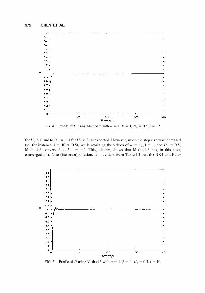
for U0 � 0 and to U� � �1 for U0 0, as expected. However, when the step size was increased(to, for instance, l � 10 � 0.5), while retaining the values of � � 1, � � 1, and U0 � 0.5,Method 3 converged to U� � �1. This, clearly, shows that Method 3 has, in this case,converged to a false (incorrect) solution. It is evident from Table III that the RK4 and Euler


FIG. 5. Profile of U using Method 3 with � � 1, � � 1, U0 � 0.5, l � 10.

372 CHEN ET AL.

methods failed for large initial conditions (in magnitude). Method 2, on the other hand, wasunaffected by the sizes of the step size or initial conditions (see Tables I and III). These resultsfurther confirm the superior convergence properties of the nonstandard method (Method 2) ascompared with the other methods.


FIG. 7. Profile of U using RK4 with � � 4, � � 1, U0 � 0.5, l � 0.5.


2.4.3. Effect of � To monitor the effect of the parameter � on the various numerical methods,we simulated the four methods (Methods 1, 2, 3, and RK4) using l � 0.5, U0 � 0.5, � � 1.0,and various values of �. The results generated by the four methods are compared in Table IV,from which it is clear that Method 2 is more robust. The RK4, for instance, exhibits chaoticdynamics (Fig. 7). The profile generated using Method 2, for � � 4, is depicted in Fig. 8.

It is worth mentioning that although the ODE45 method, a routine based on explicit RKmethods with variable step size, also works very well (like Method 2) when used to integrate themodel given by Eq. (3), its usage to solve real-life problems generally incurs substantialcomputing cost (due to the small nature of the step sizes needed). Consequently, numericalmethods that admit large step sizes, while retaining stability (such as Method 2) are more suitedfor solving real-life problems. This is especially the case for dynamical systems that requiremonitoring on a long-term basis.

3. THE NAGUMO REACTION-DIFFUSION MODEL

Consider now the full Nagumo reaction-diffusion equation

�u

�t� D

�2u

�x2 � �u � �u3, 0 � x � L, t 0, (28)

with D � 0, � � 0, � � 0, and u � u(x, t) � 0. Note that it is (realistically) assumed that thestate variable (u) and model parameters (�, �, and D) are nonnegative. That is, (28) imposes apositivity requirement. We now construct finite-difference schemes for the full Nagumo reac-tion-diffusion equation. The interval 0 x L is divided into N 1 subintervals, each of widthh, so that (N 1)h � L. The notation Um

n is used to express the solutions of the numericalmethod at the point (xm, tn).

TABLE III. Effect of U0 using � � 1, � � 1, and l � 0.5

U0 Method 1 Method 2 Method 3 RK4

�10 Overflow c3 �1 c3 �1 Overflow�2.0 c3 1 c3 �1 c3 �1 c3 �1�0.5 c3 �1 c3 �1 c3 �1 c3 �1

0.5 c3 1 c3 1 c3 1 c3 12.0 c3 �1 c3 1 c3 1 c3 1

10 Overflow c3 1 c3 1 Overflow

TABLE IV. Effect of � using U0 � 0.5, � � 1, and l � 0.5

� Method 1 Method 2 Method 3 RK4

1 c 3 ��/� c 3 ��/� c 3 ��/� c 3 ��/�1.5 c 3 ��/� c 3 ��/� c 3 ��/� c 3 ��/�2 osc c 3 ��/� c 3 ��/� c 3 ��/� c 3 ��/�4 Overflow c 3 ��/� osc c 3 ��/� Oscillation5 Overflow c 3 ��/� c 3 ��/� Chaos

10 Overflow c 3 ��/� osc c 3 ��/� Overflow

374 CHEN ET AL.

3.1. Standard Explicit Method (Method A)

A standard explicit scheme for solving (28) can be constructed by approximating the diffusionterm in (28) with its explicit central-difference approximation (CDA) given by

�2u

�x2 �Um�1

n � 2Umn � Um1

n

h2 , (29)

and the diffusion-free part by the forward-Euler method (Method 1). This gives

Umn1 � Um

n

l� D

Um�1n � 2Um

n � Um1n

h2 � �Umn � ��Um

n �3, (30)

so that

Umn1 � DPUm�1

n � �1 � �l � �l�Umn �2 � 2DP Um

n � DPUm1n , (31)

with P � l/h2. It can be shown that the principal part of the local truncation error of Method Ais O(h2 l ).

3.2. Semi-explicit Nonstandard Scheme (Method B)

The diffusion term is approximated by the same explicit CDA given by (29). The nonstandardmethod (Method 2), given by (13), is used for the diffusion-free case. This gives the followingO(h2 l ) numerical scheme for solving (28):



Umn1 � Um

n

l� D

Um�1n � 2Um

n � Um1n

h2 � ��2Umn � Um

n1� � ��Umn �2Um

n1, (32)

which can be rewritten as

�1 � �l � �l�Umn �2 Um

n1 � �1 � 2�l � 2DP�Umn � DPUm1

n � DPUm�1n (33)

Thus, solving for Umn1 gives the semi-explicit method

Umn1 �

�1 � 2�l � 2DP�Umn � DPUm1

n � DPUm�1n

1 � �l � �l�Umn �2 . (34)

Clearly, Method B, which is also O(h2 l ), satisfies the positivity property of (28) if 1 2�l �2DP � 0. Furthermore, we have the following:

Theorem 3. For any initial conditions Um0 � (0, M], the solution generated by Method B is

bounded in the interval (0, M] if 1 �l � 2DP � [(1 2�l � 2DP)2/4�lM2].Proof. To establish boundedness, we need to show that Um

n � (0, M] implies Umn1 � (0,

M]. Suppose Umn � (0, M] for some m and n. Starting with (34), we have

Umn1 �

�1 � 2�l � 2DP�Umn � DPUm1

n � DPUm�1n

1 � �l � �l�Umn �2 (35)

�1 � 2�l � 2DP�Um

n � 2DPM

1 � �l � �l�Umn �2 . (36)

Following (35), it should be noted, under the given hypothesis, that Method B satisfies thepositivity property of (28), and we only need to show that Um

n1 M. That is,

M�1 � �l � �l�Umn �2 � 2DPM � �1 � 2�l � 2DP�Um

n , (37)

so that

�l�Umn �2 �

�1 � 2�l � 2DP�Umn

M 2DP � 1 � �l. (38)

The left side of Eq. (38) reaches its minimum value, �[(1 2�l � 2DP)2/4�lM2], when Umn

� [(1 2�l � 2DP)/2�lM]. Thus, the solution generated by Method B is bounded provided

1 � �l � 2DP �1 � 2�l � 2DP�2

4�lM2 . (39)

3.3. Implicit Nonstandard Method (Method C)

Here, �2u/�x2 is approximated using the implicit CDA given by

�2u

�x2 �Um�1

n1 � 2Umn1 � Um1

n1

h2 , (40)

376 CHEN ET AL.

and the diffusion-free part is approximated by Method 2. This gives

Umn1 � Um

n

l� D

Um�1n1 � 2Um

n1 � Um1n1

h2 � ��2Umn � Um

n1� � ��Umn �2Um

n1. (41)

Equation (41) may be rearranged to get

�DPUm1n1 � DPUm�1

n1 � �1 � �l � �l�Umn �2 � 2DP Um

n1 � �1 � 2�l�Umn . (42)

Clearly, the O(h2 l ) Method C requires the application of a tri-diagonal solver at everytime-step. Note also that the matrix associated with the left-hand side (LHS) of (42) is indiagonally dominant form (for positive parameter values). The stability of the three methodsconstructed in Section 3 may be established using the matrix method (this entails finding therespective spectral norms of the associated coefficient matrices at every time step; see, forinstance, [6]).

4. NUMERICAL SIMULATIONS

In order to test the convergence properties of the three methods constructed in Section 3(Methods A, B, and C), the methods were used to solve the full Nagumo equation, given by (28),subject to the following initial conditions:

u�x, 0� � �1 for 0 � x 10 for 1 � x 2, (43)

with boundary conditions u(0, t) � 1 and u(2, t) � 0. The parameters �, �, and D were set toone. The interval 0 x 2 is subdivided into 39 subintervals, so that h � 2/40 � 0.05.

Using the aforementioned initial, boundary, and parameter values, and a time step ofl � 0.001, the three methods gave the same solution profiles at t � 1 (depicted in Fig. 9). Itshould be mentioned that using these parameter values (� � � � D � 1, h � 0.05, and l� 0.001), the positivity requirement of Method B (1 2�l � 2DP � 0.202 � 0) is satisfied.However, when the time step was increased further to l � 1, while retaining the parametervalues together with the boundary and initial data above, Method A and Method B gavedivergent solution profiles (overflow). In this case, the “positivity” requirement of Method B(1 2�l � 2DP � �798 0) is violated. Method C, on the other hand, was unaffected by theincreased size of l (Fig. 10). Further simulations with larger values of l were carried out. Theresults, summarized in Table V, confirm the robustness of the implicit nonstandard method(Method C) over the other methods.

In summary, our findings are consistent with the fact that implicit schemes, especially thosederived using the nonstandard philosophy of Mickens [4, 7, 8] (e.g., Method C), are moresuitable, in comparison to explicit schemes, for solving nonlinear initial/boundary value prob-lems.

5. CONCLUSION

We have constructed, analyzed, and simulated a number of finite-difference discretizations forthe diffusion-free Nagumo equation. In all the numerical simulations carried out, the nonstand-


ard Method 2 was seen to be more robust, i.e., had exactly the same stability features as theoriginal differential equation it approximates, in comparison wit all the other finite-differencemethods considered in Section 2, even though some of these other methods are of higher-orderin accuracy. It is important to observe that the nonstandard scheme satisfied the positivity

FIG. 9. Profile of U at t � 1 using Methods A, B, and C with � � 1, � � 1, D � 1, l � 0.001, h � 0.05.

FIG. 10. Profile of U at t � 100 using Method C with � � � � D � l � 1, h � 0.05.

378 CHEN ET AL.

requirement as demanded for the physical solutions to the original Nagumo partial differentialequation. The method was then extended and used to construct a semi-explicit and an implicitnonstandard methods for solving the full Nagumo reaction-diffusion model. Conditions forpositivity and boundedness of the semi-explicit numerical method was established. In summary,we have used nonstandard finite difference methods to construct schemes for both the diffu-sionless and full Nagumo equations such that they are dynamically consistent with the originalequations.

The authors are grateful to the reviewers for their constructive comments, which haveenhanced the article.

References

1. N. F. Britton, Reaction-diffusion equations and their applications to biology, Academic Press, NewYork, 1986.

2. E. H. Twizell, A. B. Gumel, and Q. Cao, A second-order scheme for the “Brusselator” reaction-diffusion system, Math Chem 26 (1999), 297–316.

3. A. B. Gumel and E. H. Twizell, A second-order, chaos-free, numerical method for the solution of areaction-diffusion equation in two space dimensions. Int J Non-linear Sci Numer Simul, to appear.

4. R. E. Mickens, Nonstandard finite difference schemes for reaction-diffusion equations. Numer Meth-ods Partial Differential Eq 15 (1999), 201–224.

5. A. R. Mitchell and J. C. Brunch, A numerical study of chaos in a reaction-diffusion equation, NumerMethods Partial Differential Eq 1 (1985), 13–23.

6. J. D. Lambert, Numerical methods for ordinary differential systems, the initial value problem, JohnWiley, New York, 1991.

7. R. E. Mickens, Nonstandard finite-difference models of differential equations, World Scientific,Singapore, 1994.

8. R. E. Mickens, Applications of nonstandard finite-difference schemes, World Scientific, River Edge,NJ, 2000.

9. K. T. Alligood, T. D. Sauer, and J. A. Yorke, Chaos, an introduction to dynamical systems, Springer,New York, 1997.

10. F. Verhulst, Nonlinear differential equations and dynamical systems, Springer-Verlag, Berlin, 1990.

11. R. L. Devaney, An introduction to chaotic dynamical systems, 2nd edition, Addison-Wesley Publish-ing Company, Reading, MA, 1989.

TABLE V. Effect of time step l with D � 1.

l Method A Method B Method C

0.001 Convergence Convergence Convergence0.01 Overflow Overflow Convergence0.1 Overflow Overflow Convergence1 Overflow Overflow Convergence

10 Overflow Overflow Convergence


Nonstandard discretizations of the generalized Nagumo reaction-diffusion equation

Documents

Transcript of Nonstandard discretizations of the generalized Nagumo reaction-diffusion equation