Nonparametric Predictive Inference for System...
103
Nonparametric Predictive Inference for System Reliability Ahmad M. Aboalkhair A thesis presented for the degree of Doctor of Philosophy Department of Mathematical Sciences University of Durham England May 2012
Transcript of Nonparametric Predictive Inference for System...

Nonparametric Predictive Inference for
System Reliability
Ahmad M. Aboalkhair
A thesis presented for the degree of
Doctor of Philosophy
Department of Mathematical Sciences
University of Durham
England
May 2012

Dedicated
To my father
Who has been a great source of motivation and endless support in my life
Thank you for all your sacrifices for me to help me become what I am now
To the soul of my mother
For all unlimited love, sacrifices, inspiration, prayers and faith in me
I wish I could kiss her hand and tell her how much I appreciate that
To my wife
For her endless love, support, encouragement and belief in me
Thank you for being there during the hardest of times
To my lovely children
for lighting up my life with their smile
To my brothers and sisters
for all the love, prayers and best wishes throughout my life
Nonparametric Predictive Inference for
System Reliability
Ahmad M. Aboalkhair
Submitted for the degree of Doctor of Philosophy
May 2012
Abstract
This thesis provides a new method for statistical inference on system reliability on
the basis of limited information resulting from component testing. This method
is called Nonparametric Predictive Inference (NPI). We present NPI for system
reliability, in particular NPI for k-out-of-m systems, and for systems that consist of
multiple ki-out-of-mi subsystems in series configuration. The algorithm for optimal
redundancy allocation, with additional components added to subsystems one at a
time is presented. We also illustrate redundancy allocation for the same system in
case the costs of additional components differ per subsystem.
Then NPI is presented for system reliability in a similar setting, but with all
subsystems consisting of the same single type of component. As a further step in
the development of NPI for system reliability, where more general system structures
can be considered, nonparametric predictive inference for reliability of voting sys-
tems with multiple component types is presented. We start with a single voting
system with multiple component types, then we extend to a series configuration
of voting subsystems with multiple component types. Throughout this thesis we
assume information from tests of nt components of type t.

Declaration
The work in this thesis is based on research carried out at the Department of Mathe-
matical Sciences, Durham University, UK. No part of this thesis has been submitted
elsewhere for any other degree or qualification and it is all the author’s original work
unless referenced to the contrary in the text.
Copyright© 2012 by Ahmad M. Aboalkhair.
“The copyright of this thesis rests with the author. No quotations from it should be
published without the author’s prior written consent and information derived from
it should be acknowledged”.
iv

Acknowledgements
First and foremost, all thanks and praise to Allah Almighty for his countless blessings
he has bestowed on me generally and in accomplishing this thesis especially.
I would like to express my deepest gratitude to my supervisor Prof. Frank
Coolen. To work with him is a real pleasure to me. He is always patient and en-
couraging in times of new ideas and difficulties. He listens to my ideas and discus-
sions with him frequently lead to key insights. His ability to select and to approach
compelling research problems, his high scientific standards, and his hard work set
an example. I admire his ability to balance research interests and personal pursuits.
Above all, he made me feel a friend, which I appreciate from my heart. It is very
hard to find the words to express my appreciation for him. Actually, without his
help and guidance this work would not have been possible.
I would like also to express my immense gratitude to my second supervisor, Dr.
Iain MacPhee. To my great sadness, Iain MacPhee passed away in January 2012
following a long standing battle with cancer. He was an excellent supervisor. He
patiently taught me so much that has enriched my knowledge, and I wish I could
tell him how much I appreciate that.
My final thanks go to everyone who has assisted me, stood by me or contributed
to my educational progress in any way.
v

Contents
Abstract iii
Declaration iv
Acknowledgements v
1 Introduction 1
1.1 Imprecise probability . . . . . . . . . . . . . . . . . . . . . . . . . . . 2
1.2 Nonparametric predictive inference . . . . . . . . . . . . . . . . . . . 3
1.3 k-out-of-m systems . . . . . . . . . . . . . . . . . . . . . . . . . . . . 4
1.4 Outline of thesis . . . . . . . . . . . . . . . . . . . . . . . . . . . . . . 8
2 Series of independent voting subsystems 10
2.1 Introduction . . . . . . . . . . . . . . . . . . . . . . . . . . . . . . . . 10
2.2 NPI for Bernoulli quantities . . . . . . . . . . . . . . . . . . . . . . . 11
2.3 NPI for a k-out-of-m system . . . . . . . . . . . . . . . . . . . . . . . 14
2.3.1 Examples of k-out-of-m systems . . . . . . . . . . . . . . . . . 16
2.4 Series of independent ki-out-of-mi subsystems . . . . . . . . . . . . . 18
2.5 Redundancy allocation . . . . . . . . . . . . . . . . . . . . . . . . . . 22
2.5.1 Redundancy allocation algorithm . . . . . . . . . . . . . . . . 22
2.5.2 Optimality of redundancy allocation algorithm . . . . . . . . . 24
2.6 Redundancy allocation with component costs . . . . . . . . . . . . . 29
2.7 Concluding remarks . . . . . . . . . . . . . . . . . . . . . . . . . . . . 32
3 Subsystems consisting of one type of component 34
3.1 Introduction . . . . . . . . . . . . . . . . . . . . . . . . . . . . . . . . 34
vi

Contents vii
3.2 Series of subsystems consisting of single-type components . . . . . . . 35
3.2.1 Two subsystems . . . . . . . . . . . . . . . . . . . . . . . . . 35
3.2.2 L ≥ 2 subsystems . . . . . . . . . . . . . . . . . . . . . . . . 37
3.3 Examples . . . . . . . . . . . . . . . . . . . . . . . . . . . . . . . . . 39
3.4 Concluding remarks . . . . . . . . . . . . . . . . . . . . . . . . . . . 47
4 Voting systems with multiple component types 48
4.1 Introduction . . . . . . . . . . . . . . . . . . . . . . . . . . . . . . . . 48
4.2 Multiple component types . . . . . . . . . . . . . . . . . . . . . . . . 50
4.2.1 System description . . . . . . . . . . . . . . . . . . . . . . . . 50
4.2.2 NPI lower and upper probabilities for functioning of the system 51
4.2.3 Derivation of the NPI lower and upper probabilities for func-
tioning of the system . . . . . . . . . . . . . . . . . . . . . . . 53
4.2.4 Redundancy allocation . . . . . . . . . . . . . . . . . . . . . . 55
4.3 Examples . . . . . . . . . . . . . . . . . . . . . . . . . . . . . . . . . 57
4.4 Concluding remarks . . . . . . . . . . . . . . . . . . . . . . . . . . . 64
5 Subsystems with multiple component types 66
5.1 Introduction . . . . . . . . . . . . . . . . . . . . . . . . . . . . . . . . 66
5.2 Subsystems with multiple component types . . . . . . . . . . . . . . 67
5.3 2 subsystems with 2 component types . . . . . . . . . . . . . . . . . 69
5.4 L subsystems with T component types . . . . . . . . . . . . . . . . . 70
5.5 Examples . . . . . . . . . . . . . . . . . . . . . . . . . . . . . . . . . 77
5.6 Concluding remarks . . . . . . . . . . . . . . . . . . . . . . . . . . . 81
6 Conclusions 83
Appendix 89
A Brief guide to notation 89
Bibliography 90

Chapter 1
Introduction
In classical reliability theory most of the methods and models use precise probabili-
ties to quantify uncertainty, assuming completeness of the probabilistic information
about the system and component reliability behaviour. Walley [57] discussed many
reasons why precise probability is too restrictive for practical uncertainty quantifi-
cation. In reliability, the most important ones include limited knowledge and infor-
mation about random quantities of interest, and possibly information from several
sources which might appear to be conflicting if restricted to precise probabilities.
During the past few decades, several alternative methods for uncertainty quan-
tification have been proposed, some also for reliability. For example, fuzzy reliability
theory [11] and possibility theory [32] provided solutions to problems that could not
be solved satisfactorily with precise probabilities. The theory of imprecise probabil-
ities [57] and the theory of interval probability [59] have been used as a general and
promising tool for reliability analysis. Coolen [13] provided an insight into impre-
cise reliability, discussing a variety of issues and reviewing suggested applications
of imprecise probabilities in reliability, see [54] for a detailed overview of imprecise
reliability and many references.
In this thesis a statistical approach which uses imprecise probability is presented
for system reliability. This approach is called Nonparametric Predictive Inference
(NPI). It provides a new method for statistical inference on system reliability on the
basis of limited information resulting from component testing.
1

1.1. Imprecise probability 2
Section 1.1 provides a brief introduction to imprecise probability, which is an
umbrella term encompassing all qualitative and quantitative ways of measuring un-
certainty without single-valued probabilities. In Section 1.2 we review briefly the
main idea of NPI. The class of k-out-of-m systems and a brief overview of some
recent contributions that focus on reliability of this class of systems is presented in
Section 1.3. The outline of this thesis is given in Section 1.4.
1.1 Imprecise probability
The idea to use interval-valued probabilities dates back at least to the middle of the
nineteenth century [10]. In recent years this has particularly been a growing area of
research. Researchers with widely varying backgrounds are currently contributing
to theory, and indeed applications, of imprecise probability, including mathemati-
cians, statisticians, computer scientists, and researchers working on artificial intel-
ligence, medicine, and a variety of engineering areas. Such researchers are brought
together via the Society for Imprecise Probability Theory and Applications (SIPTA,
http://www.sipta.org), which also organizes biennial conferences.
In classical probability theory, a single probability P (A) ∈ [0, 1] is used to
quantify uncertainty about an event A. Lower and upper probabilities general-
ize the standard theory of (‘single-valued’ or ‘precise’) probability and provide a
powerful method for uncertainty quantification [54]. The main idea is that, for an
event A, lower probability P (A) ∈ [0, 1] and upper probability P (A) ∈ [0, 1] with
0 ≤ P (A) ≤ P (A) ≤ 1 are specified, such that these lower and upper probabilities
define a so-called ‘structure’ M, which is a set of precise probability distributions
corresponding to the lower and upper probabilities in the sense that for each prob-
ability distribution P (·) ∈ M, P (A) ≤ P (A) ≤ P (A) and P (A) = infP (·)∈M P (A)
and P (A) = supP (·)∈M P (A) [8]. The classical situation of precise probability occurs
if P (A) = P (A), whereas P (A) = 0 and P (A) = 1 represents complete lack of
knowledge about A. These lower and upper probabilities are naturally linked by the
conjugacy property P (A) = 1−P (Ac) [8]. This generalization allows indeterminacy
about A to be taken into account, and lower and upper probabilities can also be
1.2. Nonparametric predictive inference 3
interpreted in several ways. One can consider them as bounds for a precise proba-
bility, related to relative frequency of the event A, reflecting the limited information
one has about A. Generally, P (A) reflects the information and beliefs in favour of
event A, while P (A) reflects such information and beliefs against A, so in favour of
Ac.
Coolen [12] presented lower and upper predictive probabilities for Bernoulli ran-
dom quantities. These lower and upper probabilities are part of a wider statistical
methodology called ‘Nonparametric Predictive Inference’ (NPI), which is a frequen-
tist statistical approach with strong consistency properties in the theory of imprecise
probability [8].
1.2 Nonparametric predictive inference
Nonparametric predictive inference (NPI) is a statistical method to learn from data
in the absence of prior knowledge and using only few modelling assumptions. It
provides a solution to some explicit goals for objective (Bayesian) inference, for
example the empirical and logical norms as formulated by Williamson [60]. These
goals cannot be obtained when using precise probabilities, but are achieved by NPI
after slight reformulation to allow the use of lower and upper probabilities [14]. It
is also exactly calibrated [39], which is a strong consistency property in frequentist
statistics, and it never leads to results that are in conflict with inferences based on
empirical probabilities.
NPI is based on Hill’s assumption A(n) [35], which gives direct probabilities [31]
for a future observable random quantity, based on observed values of n related
random quantities. Suppose that X1, · · · , Xn, Xn+1 are continuous and exchangeable
random quantities. So, for one such a random quantity, its rank among all these
random quantities is uniformly distributed over the values 1 to n + 1 (assuming no
ties for simplicity). Let the ordered observed values of X1, · · · , Xn be denoted by
x(1) < x(2) < · · · < x(n) < 1, and let x(0) = −∞ and x(n+1) = ∞ for ease of notation.
For a future observation Xn+1, based on n observations, A(n) is
P (Xn+1 ∈ (xj−1, xj)) =1
n + 1j = 1, 2, · · · , n + 1
1.3. k-out-of-m systems 4
A(n) does not assume anything else, and can be considered to be a post-data as-
sumption related to exchangeability [30]. For a detailed discussion of A(n) we refer
to Hill [36]. Inferences based on A(n) are predictive and nonparametric, and are suit-
able if there is hardly any knowledge about the random quantity of interest, other
than the first n observations, or if one does not want to use such information, for
example to study effects of additional assumptions underlying other statistical meth-
ods. Nevertheless, A(n) has not received much attention in the statistical literature.
A logical reason is that it only assigns equal probabilities for the next observation to
belong to each of the n + 1 intervals created by the previous n observations, so very
few inferences can be based on this without requiring additional assumptions. How-
ever, it provides bounds for probabilities for all events of interest involving Xn+1.
These bounds follow from De Finetti’s fundmental theorem of probability [30] and
are the sharpest bounds for all events, corresponding to the probabilities defined by
the assumption A(n). Consequently, these are lower and upper probabilities in the
theory of imprecise probability.
NPI is a framework of statistical theory and methods that use these A(n)-based
lower and upper probabilities. It has been presented for Bernoulli data [12], real-
valued data [8], data including right-censored observations [25] and multinomial
data [21,22]. NPI has a wide range of applications in statistics, operational research
and reliability [17]. For example, applications of NPI to basic problems in reliability
include reliability demonstration for failure-free periods [23], (opportunity-based)
age replacement [26,27], comparison of success-failure data [28], probabilistic safety
assessment in case of zero failures [15], and prediction of not yet observed failure
modes [16]. In this thesis, we are interested in NPI for system reliability, in particular
NPI for k-out-of-m systems, and for systems that consist of multiple ki-out-of-mi
subsystems in series configuration [18,19,42].
1.3 k-out-of-m systems
The class of k-out-of-m systems, also called ‘voting systems’, was introduced by
Birnbaum [9]. These are systems that consist of m exchangeable components (often

1.3. k-out-of-m systems 5
the confusing term identical components is used), such that the system functions if
and only if at least k of its components function. Since the value of m is usually
larger than the value of k, redundancy is generally built into a k-out-of-m system.
Both parallel and series systems are special cases of the k-out-of-m system. A series
system is equivalent to an m-out-of-m system while a parallel system is equivalent
to an 1-out-of-m system.
Throughout this thesis, we use the term ‘exchangeable components’ to indicate
the scenario required for application of A(n) as described in Sections 1.2 and 2.2.
Effectively, exchangeable components are ‘similar’ with regard to our knowledge
about their functioning. In practice, this may typically apply to components which
are manufactured in the same process and which have similar roles in the system
which is being considered. Information about the quality of components is assumed
to come from testing of further components which are exchangeable with those in the
system. Therefore, this would typically require that tests take place under similar
circumstances as will apply to the functioning of the components in the system.
Applications of k-out-of-m systems can e.g. be found in the areas of target detec-
tion, communication, safety monitoring systems, and, particularly, voting systems.
The k-out-of-m systems are a very common type in fault-tolerant systems with re-
dundancy. They have many applications in both industrial and military systems.
Fault-tolerant systems include the multi-display system in a cockpit, the multi-
engine system in an airplane, and the multi-pump system in a hydraulic control
system [52]. For example, a car with a V 8 engine may be driven if only four cylin-
ders are firing. But, if less than four cylinders fire, then the car cannot be driven.
Thus, the functioning of the engine can be considered as a 4-out-of-8 system. The
system is tolerant of failures of up to four cylinders for minimal functioning of the en-
gine [38]. In a data processing system with five video displays, a minimum of three
displays operable may be sufficient for full data display. In this case the display
system functions as a 3-out-of-5 system. In a communications system with three
transmitters, the average message load may be such that at least two transmitters
must be operational at all times, or else critical messages may be lost. Thus, the
transmission system behaves as a 2-out-of-3 system. Systems with spares may also

1.3. k-out-of-m systems 6
be represented by a k-out-of-m system model. A car with four tires, for example,
usually has one additional spare tire. Thus, the vehicle can be driven as long as at
least 4-out-of-5 tires are in good condition [38].
A traditional problem considered in reliability theory is assessment of system
reliability [7], where voting systems have received particular attention. Many recent
contributions to the literature focus on reliability of the class of k-out-of-m systems,
albeit from a classical perspective using precise probabilities to quantify uncertainty.
For example, Torres-Echeverria et al. [53] address modelling of probability of dan-
gerous failure on demand and spurious trip rate of safety instrumented systems that
include k-out-of-m voting redundancies in their architecture. Senz-de-Cabezn et al.
[49] presented computational algebraic algorithms for the reliability of generalized
k-out-of-m and related systems. They analysed and computed identities and bounds
for the reliability of coherent systems using the techniques of commutative algebra.
They applied the techniques to the analysis of some of the most relevant k-out-of-m
systems. They concluded that the efficiency of their approach in obtaining exact
identities, bounds and asymptotic formulas shows good performance when compared
with others results from the literature.
Moghaddass et al. [45] consider a general repairable k-out-of-m system with
non-identical components that can have different repair priorities. They address
the problem of efficient evaluation of the system’s availability in a way that steady
state solutions can be obtained systematically with reasonable computation time.
Vaurio [56] considers the unavailability of redundant standby systems with k-out-
of-m logic. Such systems are subject to latent failures that are detected by periodic
tests and repaired immediately after discovery. He considers many potential failure
and error modes in the formalism, evaluates both consecutive and staggered testing
schemes and suggests methods for including common cause failures in the analyses.
Levitin [40] proposes a model that generalizes linear consecutive k-out-of-r-from-m
systems to linear n-gap-consecutive k-out-of-r-from-m : F systems. In this model
the system consists of m linearly ordered statistically independent identical elements
and fails if the gap between any pair of groups of r consecutive elements containing
at least k failed elements is less than n elements.

1.3. k-out-of-m systems 7
Erylmaz [33] studied circular consecutive k-out-of-m systems consisting of ex-
changeable components. He derived explicit expressions for both unconditional and
conditional survival functions for 2k + 1 ≥ m, while signature-based mixture repre-
sentations for general k are obtained. Salehi et al. [50] considered linear and circular
consecutive k-out-of-m systems. It is assumed that lifetimes of components of the
systems are independent but their probability distributions are non-identical. The
reliability properties of the residual lifetimes of such systems under the condition
that at least m−r+1, with r ≤ m, components of the system are operating was stud-
ied. The probability that a specific number of components of the above-mentioned
system operate at time t, t > 0, under the condition that the system is alive at
time t was also investigated. Gurler and Capar [34] established an algorithm for
the computation of the mean residual lifetime of an (m− k + 1)-out-of-m system in
the case of independent but not necessarily identically distributed lifetimes of the
components. They gave an application for the exponentiated Weibull distribution
to study the effect of various parameters on the mean residual lifetime of the sys-
tem. The relationship between the mean residual lifetime for the system and that
of its components was also investigated. Ruiz-Castro and Li [48] presented an algo-
rithm for a general discrete voting system subject to several types of failure with an
indefinite number of repairpersons. The model is built and the stationary distribu-
tion, for the general case, is derived using matrix-analytic methods. They computed
performance measures of interest for the transient and the stationary regime, includ-
ing availability, reliability and the conditional probability of failure for the different
types of failures and for the system.
These recent papers are evidence of the continuing importance of development
of methodology to quantify system reliability. The NPI approach presented in this
thesis provides the important opportunity to reflect, by the use of lower and upper
probabilities, the fact that information from tests is often quite limited.

1.4. Outline of thesis 8
1.4 Outline of thesis
In this thesis, we present important extensions for the NPI approach to system re-
liability. Coolen-Schrijner et al. [29] considered NPI for system reliability, and in
particular for series systems with subsystem i a ki-out-of-mi system. They presented
an attractive algorithm for optimal redundancy allocation, with additional compo-
nents added to subsystems one at a time. However, they only proved this result
for test data with no failed components. We start with generalising the algorithm
for redundancy allocation presented by Coolen-Schrijner et al. [29] to general test
results, a situation in which redundancy plays an even more important role than
when testing revealed no failures at all. We also illustrate redundancy allocation for
the same system in case the costs of additional components differ per subsystem.
Then NPI is presented for system reliability in a similar setting, but with all sub-
systems consisting of the same single type of component. As a further step in the
development of NPI for system reliability, where more general system structures can
be considered, nonparametric predictive inference for reliability of voting systems
with multiple component types is presented. We start with a single voting system
with multiple component types, then we extend to a series configuration of voting
subsystems with multiple component types. Throughout this thesis we assume in-
formation from tests of nt components of type t. All computations were performed
using R. Some parts of this thesis have been presented at conferences and related
papers have been published in academic journals or are in submission [1–6,18,19,42].
Chapter 2 begins with a brief overview of NPI for Bernoulli data, using a path
counting technique to compute upper and lower probabilities. We present the main
results on NPI for k-out-of-m systems, and these results are illustrated and discussed
via examples. We provide a detailed presentation of optimal redundancy allocation
following general component test results and the proofs of the main results. We
present another extension for the NPI approach to system reliability, namely inclu-
sion of different costs per component of the different types. Part of this chapter
was presented at the 18th Advances in Risk and Reliability Technology Symposium
(Loughborough, UK, 2009) [1].
1.4. Outline of thesis 9
In Chapter 3, we consider NPI for system reliability in a similar setting, but with
all subsystems consisting of the same single type of component. Such components
are exchangeable with regard to the information about them contained in test results
but they play different roles in the system if they are in different subsystems. NPI
lower and upper probabilities for a series of two ki-out-of-mi subsystems consisting
of single-type components are derived. These results are generalized to systems
with L ≥ 2 ki-out-of-mi subsystems in a series configuration. This chapter was
presented (by Frank Coolen) at a symposium in remembrance of Professor Jan M.
van Noortwijk (Delft, the Netherlands, 2009) [18].
In Chapter 4, we consider more general system structures. Whilst restricting
attention to a single voting system, this can now consist of multiple types of com-
ponents. They are assumed to all play the same role within the system, but with
regard to their reliability components of different types are assumed to be indepen-
dent. This chapter was presented at the International Conference on Accelerated
Life Testing, Reliability-based Analysis and Design: ALT2010 (Clermont-Ferrand,
France, 2010) [2].
In Chapter 5, we generalize the results introduced in Chapters 2, 3 and 4 by
considering systems in series structure where each subsystem is a voting system with
multiple types of components and with components of the same type appearing in
different subsystems. A part of Chapter 5 was presented at the 19th Advances in
Risk and Reliability Technology Symposium (Stratford-upon-Avon, UK, 2011) [3],
and a comprehensive overview of Chapter 5 and the main parts of this thesis was
presented at the European Safety & Reliability Conference - ESREL 2011 (Troyes,
France, 2011) [4].
In Chapter 6, we discuss opportunities to extend the research presented in this
thesis, which is also discussed in the final sections of each of Chapters 2 to 5.
Although the most general results in Chapter 5 contain the results of Chapters
2, 3 and 4 as special cases, the presentation in this thesis reflects the progress
of the research project over time and in every step a substantial problem is solved,
hence this order of detailed presentation provides much insight into the complexities
involved.
Chapter 2
Series of independent voting
subsystems
2.1 Introduction
Coolen-Schrijner et al. [29] considered NPI for system reliability, and in particular
for series systems with subsystem i a ki-out-of-mi system. Such systems are com-
mon in practice, and can offer the important advantage of building in redundancy
by increasing some mi to increase the system reliability. Coolen-Schrijner et al. [29]
applied NPI for Bernoulli data [12] to such systems, with inferences on each sub-
system i based on information from tests on ni components, with the components
tested assumed to be exchangeable with the corresponding components to be used
in that subsystem. Coolen-Schrijner et al. [29] presented an attractive algorithm for
optimal redundancy allocation, with additional components added to subsystems
one at a time, which in their setting was proven to be optimal. Hence, NPI for
system reliability provides a very tractable model, which greatly simplifies optimi-
sation problems involved with redundancy allocation. However, they only proved
this result for tests in which no components failed. In this chapter, this result is
generalized for redundancy allocation following tests in which any number of com-
ponents can have failed, a situation in which redundancy possibly plays an even
more important role than when testing revealed no failures at all.
10

2.2. NPI for Bernoulli quantities 11
Section 2.2 presents a brief overview of NPI, and particularly of NPI for Bernoulli
data using a path counting technique to compute upper and lower probabilities.
Section 2.3 presents the main results on NPI for k-out-of-m systems [29], and these
results are illustrated and discussed via examples. Section 2.4 extends this approach
to systems which are series of independent subsystems, with each subsystem a ki-
out-of-mi system with exchangeable components. Section 2.5 provides a detailed
presentation of optimal redundancy allocation following general component test re-
sults and the proof of optimality. Section 2.6 presents another extension for the NPI
approach to system reliability, namely the optimization of system reliability under
cost considerations. Section 2.7 contains some concluding remarks.
2.2 NPI for Bernoulli quantities
In this section, NPI for Bernoulli random quantities [12] is summarized, together
with the key results for NPI for system reliability by Coolen-Schrijner et al. [29].
Suppose that there is a sequence of n + m exchangeable Bernoulli trials, each with
‘success’ and ‘failure’ as possible outcomes, and data consisting of s successes in
n trials. Let Y n1 denote the random number of successes in trials 1 to n, then a
sufficient representation of the data for the inferences considered is Y n1 = s, due
to the assumed exchangeability of all trials. Let Y n+mn+1 denote the random number
of successes in trials n + 1 to n + m. Let Rt = {r1, . . . , rt}, with 1 ≤ t ≤ m + 1
and 0 ≤ r1 < r2 < . . . < rt ≤ m, and, for ease of notation, define(
s+r0
s
)= 0.
Then the NPI upper probability for the event Y n+mn+1 ∈ Rt, given data Y n
1 = s, for
s ∈ {0, . . . , n}, is
P (Y n+mn+1 ∈ Rt|Y n
1 = s) =(n + m
n
)−1
×t∑
j=1
[(s + rj
s
)−(
s + rj−1
s
)](n − s + m − rj
n − s
)The corresponding NPI lower probability can be derived via the conjugacy property
P (Y n+mn+1 ∈ Rt|Y n
1 = s) = 1 − P (Y n+mn+1 ∈ Rc
t |Y n1 = s)
where Rct = {0, 1, . . . , m}\Rt.

2.2. NPI for Bernoulli quantities 12
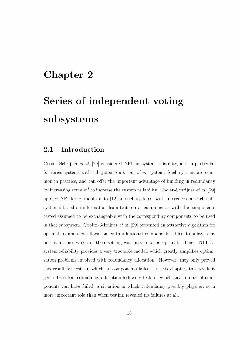
(0,0)n
m (n,m)
Figure 2.1: All possible paths from (0,0) to (n,m)
Coolen [12] derived these NPI lower and upper probabilities through direct count-
ing arguments. The method uses the appropriate A(n) assumptions [35] for inference
on m future random quantities given n observations, and a latent variable represen-
tation with Bernoulli quantities represented by observations on the real line, with
a threshold such that successes are to one side and failures to the other side of the
threshold. Under these assumptions, the(
n+mn
)different orderings of these obser-
vations, when not distinguishing between the n observed values nor between the m
future observations, are all equally likely. For each such an ordering, the success-
failure threshold can be in any of the n + m + 1 intervals of the partition of the real
line created by the n+m values of the latent variables, leading to n+m+1 possible
combinations (s, r), with s successes in the n tests and r successes in the m future
observations.
For such an ordering, these possible (s, r) can be represented as a path on the
rectangular lattice from (0, 0) to (n,m) with steps going either one to the right
or one upwards (see Figure 2.1). The(
n+mn
)different orderings, which are all
equally likely, correspond to the(
n+mn
)different right-upwards paths from (0, 0) to
(n,m), and hence the above NPI lower and upper probabilities can also be derived
by counting paths. To derive the NPI lower probability P (Y n+mn+1 ∈ Rt|Y n
1 = s),
one counts all such paths which for given s must go only through points (s, r) with
2.2. NPI for Bernoulli quantities 13
k
(0,0) s−1 s n
m (n,m)
Figure 2.2: all paths from (0,0) to (n,m) that pass through (s− 1, k) and (s + 1, k)
s n
(n,m)
(0,0)
k
m
Figure 2.3: All paths from (0,0) to (n,m) via (s, k)
r ∈ Rt, so they do not go through (s, l) for any l ∈ Rct . The corresponding NPI
upper probability P (Y n+mn+1 ∈ Rt|Y n
1 = s) is derived by counting all such paths that
go through at least one (s, r) with r ∈ Rt. For example, the NPI lower probability
for the event (Y n+mn+1 = k | Y n
1 = s) can be derived by counting the paths from (0,0)
to (n,m) that pass through the two points (s− 1, k) and (s + 1, k) respectively (see
Figure 2.2). The number of these paths is(
s−1+ks−1
)(n−s−1+m−k
m−k
), hence
P (Y n+mn+1 = k | Y n
1 = s) =
(n + m
n
)−1 [(s − 1 + k
s − 1
)(n − s − 1 + m − k
m − k
)]The corresponding NPI upper probability can be derived by counting all paths
from (0,0) to (n,m) via (s, k) (see Figure 2.3). The number of these paths is(s+k
s
)(n−s+m−k
n−s
), hence
P (Y n+mn+1 = k | Y n
1 = s) =
(n + m
n
)−1 [(s + k
s
)(n − s + m − k
n − s
)]
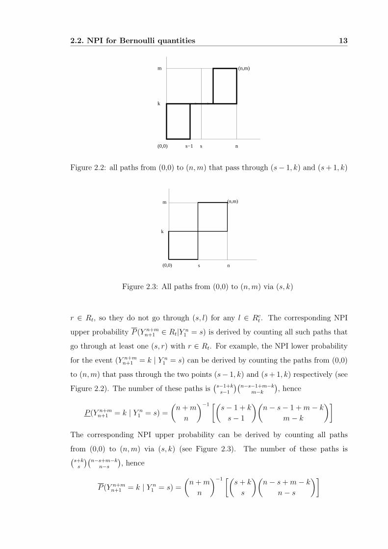
2.3. NPI for a k-out-of-m system 14
+ + ... +
0 0 0
(n,m) (n,m) (n,m)
k kk
k+1k+1 k+1
s s ss−1 s−1s−1
m
n
m
n n
m
Figure 2.4: All paths which are counted in the upper probability (2.1)
In the next section, these results of NPI for Bernoulli data, are used to compute
upper and lower probabilities for successful functioning of k-out-of-m systems.
2.3 NPI for a k-out-of-m system
When considering a k-out-of-m system, the event Y n+mn+1 ≥ k is of interest as this
corresponds to successful functioning of a k-out-of-m system, following n tests of
components that are exchangeable with the m components in the system considered.
Given data consisting of s successes from n components tested, the NPI lower and
upper probabilities for the event that the k-out-of-m system functions successfully
are also denoted by P (S(m : k)| (n, s)) and P (S(m : k)| (n, s)), respectively. From
the NPI upper probability for Y n+mn+1 ∈ Rt given above, P (S(m : k)| (n, s)) follows
easily. For k ∈ {1, 2, . . . , m} and 0 < s < n,
P (S(m : k)| (n, s)) = P (Y n+mn+1 ≥ k|Y n
1 = s) =
(n + m
n
)−1
×[(s + k
s
)(n − s + m − k
n − s
)+
m∑l=k+1
(s + l − 1
s − 1
)(n − s + m − l
n − s
)](2.1)
This NPI upper probability can also be derived by counting all such paths that go
through at least one point (s, r) with r ≥ k. To avoid that no path is counted more
than once, the number of these paths can be computed by counting all paths from
(0,0) to (n,m) via (s, k), in addition to paths from (0,0) to (n,m) via at least one
of (s − 1, k + 1), (s − 1, k + 2), (s − 1, k + 3), . . . , (s − 1,m) (see Figure 2.4). The
2.3. NPI for a k-out-of-m system 15
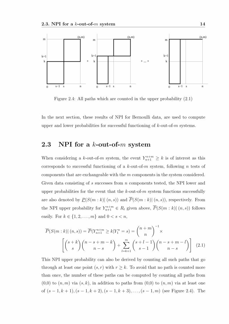
+ + ... +
0 0 0s s ss−1 s−1 s−1
k k k
k+1k+1 k+1
(n,m) (n,m) (n,m)
n
m m
n
m
n
Figure 2.5: All paths which are counted in the lower probability (2.2)
corresponding NPI lower probability can be derived via the conjugacy property or by
counting all paths which go through (s, r) for r ≥ k but not through any point (s, r)
with r less than k. The number of these paths is equal to the number of paths from
(0,0) to (n,m) via at least one of (s−1, k), (s−1, k +1), (s−1, k +2), . . . , (s−1,m)
(see Figure 2.5).
P (S(m : k)| (n, s)) = P (Y n+mn+1 ≥ k|Y n
1 = s) = 1 − P (Y n+mn+1 ≤ k − 1|Y n
1 = s)
= 1 −(
n + m
n
)−1[
k−1∑l=0
(s + l − 1
s − 1
)(n − s + m − l
n − s
)](2.2)
For m = 1, so considering a system consisting of just a single component, the NPI
upper and lower probabilities for the event that the system functions successfully
are
P (S(1 : 1)| (n, s)) = P (Y n+1n+1 = 1|Y n
1 = s) =s + 1n + 1
P (S(1 : 1)| (n, s)) = P (Y n+1n+1 = 1|Y n
1 = s) =s
n + 1
If the observed data are all successes, so s = n, or all failures, so s = 0, then the
NPI upper probabilities are, for all k ∈ {1, . . . , m},
P (S(m : k)| (n, n)) = P (Y n+mn+1 ≥ k|Y n
1 = n) = 1
P (S(m : k)| (n, 0)) = P (Y n+mn+1 ≥ k|Y n
1 = 0) =(
n + m − k
n
)(n + m
n
)−1
and the NPI lower probabilities are, for all k ∈ {1, . . . , m},
P (S(m : k)| (n, n)) = P (Y n+mn+1 ≥ k|Y n
1 = n) = 1 −(
n + k − 1n
)(n + m
n
)−1
P (S(m : k)| (n, 0)) = P (Y n+mn+1 ≥ k|Y n
1 = 0) = 0

2.3. NPI for a k-out-of-m system 16
n(0,0)
k
s s+1
m (n,m)
Figure 2.6: All paths which are counted in (2.3)
One of the results that actually holds generally for the NPI lower and upper
probabilities for all k-out-of-m systems as considered in this thesis is
P (S(m : k)| (n, s)) = P (S(m : k)| (n, s + 1)) (2.3)
A direct proof of (2.3) can be easily achieved by using a path counting technique.
Figure 2.6 shows that the paths that go through at least one point (s, r) with r ≥ k
(which are counted in the NPI upper probability for successful system functioning
given s successes in n tests) ara exactly the same paths that go through (s+1, r) for
r ≥ k but not through any point (s + 1, r) with r less than k (which are counted in
the NPI lower probability for successful system functioning given s + 1 successes).
2.3.1 Examples of k-out-of-m systems
In this subsection two examples are presented to illustrate NPI for reliability of
k-out-of-m systems, and some related issues are discussed.
Example 2.1
Consider a k-out-of-6 system. Table 2.1 provides the NPI lower and upper proba-
bilities for all possible cases with n = 5 components tested, of which s functioned
successfully, and with k varying from 1 to 6. The values in Table 2.1 illustrate some
of the general properties for all k-out-of-m systems. The NPI upper probability for
successful system functioning given s successes in n tests is equal to the NPI lower

2.3. NPI for a k-out-of-m system 17
k = 1 k = 2 k = 3 k = 4 k = 5 k = 6
P P P P P P P P P P P P
s = 0 0 0.545 0 0.273 0 0.121 0 0.045 0 0.013 0 0.002
s = 1 0.545 0.818 0.273 0.576 0.121 0.348 0.045 0.175 0.013 0.067 0.002 0.015
s = 2 0.818 0.939 0.576 0.803 0.348 0.608 0.175 0.392 0.067 0.197 0.015 0.061
s = 3 0.939 0.985 0.803 0.933 0.608 0.825 0.392 0.652 0.179 0.424 0.061 0.182
s = 4 0.985 0.998 0.933 0.987 0.825 0.955 0.652 0.878 0.424 0.727 0.182 0.455
s = 5 0.998 1 0.987 1 0.955 1 0.878 1 0.727 1 0.455 1
Table 2.1: NPI lower and upper probabilities for all possible cases with n = 5
probability for successful system functioning given s + 1 successes. The value 0 (1)
of the NPI lower (upper) probability for the case s = 0 (s = 5) reflects that in this
case there is no strong evidence that the components can actually function (fail).
In order to get a reasonably large NPI lower probability for successful system func-
tioning, it is not necessarily required that most tested components functioned well
if k is small, which means that the system has much built-in redundancy, but for
large values of k (nearly) all tested components must have been successful. Table
2.1 shows that the lower and upper probabilities are decreasing in k when keeping
m, n and s constant, and increasing in s when keeping m, n and k constant. This
is most obvious from the large differences between the values at the top left and
bottom right of Table 2.1.
Example 2.2
Consider a 10-out-of-m system. Suppose that, to increase the system’s reliability
by increasing redundancy, extra components can be added to the system, keeping
k = 10 but increasing the value of m. Assuming zero-failure testing, the NPI lower
probabilities for the event that this system functions successfully are presented in
Table 2.2 , for n = 5, 10, 15, 20, 25, and m varying from 10 to 15. Of course, the
corresponding NPI upper probabilities are all equal to one as there are no failed
components. Table 2.2 shows that the system’s reliability as measured by NPI
lower probability is increasing in m, keeping n and k constant, and increasing in n,
keeping m and k constant.

2.4. Series of independent ki-out-of-mi subsystems 18
m = 10 11 12 13 14 15
s = n = 5 0.333 0.542 0.676 0.766 0.828 0.871
10 0.500 0.738 0.857 0.919 0.953 0.972
15 0.600 0.831 0.925 0.965 0.983 0.992
20 0.667 0.882 0.956 0.983 0.993 0.997
25 0.714 0.913 0.972 0.990 0.997 0.999
Table 2.2: NPI lower probabilities for the systems in Example 2.2
The NPI lower probabilities presented in Table 2.2 can be used in several ways.
For example, consider the case m = 10 with 5 zero-failure tests, leading to NPI
lower probability 0.333 for successful system functioning. The table shows that
increasing the redundancy to m = 11, keeping k = 10, would increase the NPI lower
probability to 0.542, while increasing the number of zero-failure tests to 10 would
increase the NPI lower probability to 0.5, so if these two actions were available at
similar costs, increase of redundancy might be preferred to more tests. However, if
15 tests were possible at a cost similar to the cost of adding one component to the
system, then this might be preferred, as the corresponding NPI lower probability
would increase to 0.6 if all 15 tests were successes. Of course, we do not know if
extra tested components would all function successfully.
Table 2.3 extends this example by presenting the minimum number of zero-failure
tests required to achieve a chosen value for the NPI lower probability for successful
system functioning, again for k = 10 and m varying from 10 to 15. The requirement
considered is P (S(m : 10)| (n, n)) ≥ p for different values of p.
The main conclusion from Table 2.3 is that the system’s reliability, as measured
by NPI lower probability, can be increased either by having more successful tests or
by building in redundancy.
2.4 Series of independent ki-out-of-mi subsystems
Coolen-Schrijner et al. [29] used the results for a k-out-of-m system straightfor-
wardly to consider the reliability of systems that consist of a series configuration

2.4. Series of independent ki-out-of-mi subsystems 19
m = 10 11 12 13 14 15
p = 0.75 30 11 7 5 4 4
0.80 40 13 8 6 5 4
0.85 57 17 10 7 6 5
0.90 90 23 13 9 7 6
0.95 190 37 19 13 10 8
0.99 990 95 40 25 18 15
Table 2.3: Values of n required to achieve chosen values of p.
of L ≥ 2 independent subsystems, with subsystem i (i = 1, . . . , L) a ki-out-of-mi
system consisting of exchangeable components. As before, it is assumed that, in
relation to subsystem i, ni components that are exchangeable with those to be used
in the subsystem have been tested, of which si functioned successfully. For the se-
ries system to function, all its subsystems must function, and due to the assumed
independence of the subsystems (which implies independence of components in dif-
ferent subsystems), the NPI lower and upper probabilities for such a series system
to function are
P (S[L](m1 : k1, . . . ,mL : kL) | (n, s)) =L∏
i=1
P (S(mi : ki)| (ni, si)) (2.4)
and
P (S[L](m1 : k1, . . . ,mL : kL) | (n, s)) =L∏
i=1
P (S(mi : ki)| (ni, si)) (2.5)
Coolen-Schrijner et al. [29] considered optimal redundancy allocation for such
systems, that is how best to assign additional components to subsystems (hence to
increase the number of components mi), for situations where the required number of
components that must function for the subsystems remains the same (ki). However,
they only considered such redundancy allocation after zero-failure testing (so si = ni
for all i = 1, . . . , L), for which case they derived a powerful algorithm for optimal
redundancy allocation, with the lower probability for system functioning used as the
reliability measure. The NPI lower and upper probabilities for such a series system
to function are illustrated and discussed in the following example.

2.4. Series of independent ki-out-of-mi subsystems 20
(m1,m2) = (4, 4) (4, 5) (5, 5) (4, 6) (4, 7) (5, 6) (6, 6)
(s1, s2) = (1,1) 0.0000 0.0001 0.0002 0.0001 0.0002 0.0005 0.0009
(1,2) 0.0001 0.0003 0.0010 0.0006 0.0009 0.0018 0.0037
(2,1) 0.0001 0.0004 0.0010 0.0007 0.0012 0.0020 0.0037
(2,2) 0.0006 0.0016 0.0045 0.0029 0.0043 0.0081 0.0147
(3,3) 0.0051 0.0125 0.0307 0.0203 0.0274 0.0497 0.0804
(4,3) 0.0119 0.0292 0.0611 0.0473 0.0639 0.0988 0.1418
(5,3) 0.0238 0.0584 0.1009 0.0945 0.1278 0.1633 0.2062
(3,4) 0.0119 0.0249 0.0611 0.0357 0.0440 0.0877 0.1418
(3,5) 0.0238 0.0411 0.1009 0.0519 0.0586 0.1275 0.2062
(4,4) 0.0278 0.0581 0.1214 0.0833 0.1028 0.1742 0.2500
(5,4) 0.0556 0.1162 0.2006 0.1667 0.2055 0.2879 0.3636
(6,4) 0.1000 0.2091 0.2851 0.3000 0.3699 0.4091 0.4545
(4,5) 0.0556 0.0960 0.2006 0.1212 0.1368 0.2534 0.3636
(4,6) 0.1000 0.1364 0.2851 0.1515 0.1585 0.3168 0.4545
(5,5) 0.1111 0.1919 0.3315 0.2424 0.2735 0.4187 0.5289
(6,5) 0.2000 0.3455 0.4711 0.4364 0.4923 0.5950 0.6612
(5,6) 0.2000 0.2727 0.4711 0.3030 0.3170 0.5234 0.6612
(6,6) 0.3600 0.4909 0.6694 0.5454 0.5706 0.7438 0.8264
Table 2.4: NPI lower probability for system functioning
Example 2.3
Consider a system which consists of two independent subsystems (so L = 2) in
a series configuration, where for each subsystem 4 exchangeable components must
function to ensure that the subsystem functions, hence k1 = k2 = 4, and where 6
components exchangeable with those in subsystem 1 have been tested, and also 6
components exchangeable with those in subsystem 2 have been tested, so n1 = n2 =
6. Tables 2.4 and 2.5 present the NPI lower and upper probabilities, respectively,
for functioning of this system, for varying numbers of test successes (s1 and s2) and
different numbers of components (m1 and m2) in these ki-out-of-mi subsystems.
Test results for which the NPI lower probability for system functioning is zero
(s1 = 0 or s2 = 0) are deleted from Table 2.4, the case s1 = s2 = 6 is deleted from
2.4. Series of independent ki-out-of-mi subsystems 21
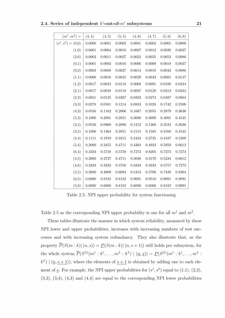
(m1, m2) = (4, 4) (4, 5) (5, 5) (4, 6) (4, 7) (5, 6) (6, 6)
(s1, s2) = (0,0) 0.0000 0.0001 0.0002 0.0001 0.0002 0.0005 0.0009
(1,0) 0.0001 0.0004 0.0010 0.0007 0.0012 0.0020 0.0037
(2,0) 0.0003 0.0011 0.0027 0.0022 0.0035 0.0053 0.0086
(0,1) 0.0001 0.0003 0.0010 0.0006 0.0009 0.0018 0.0037
(0,2) 0.0003 0.0008 0.0027 0.0014 0.0018 0.0043 0.0086
(1,1) 0.0006 0.0016 0.0045 0.0029 0.0043 0.0081 0.0147
(1,2) 0.0017 0.0042 0.0118 0.0068 0.0091 0.0190 0.0344
(2,1) 0.0017 0.0048 0.0118 0.0087 0.0128 0.0213 0.0344
(2,2) 0.0051 0.0125 0.0307 0.0203 0.0274 0.0497 0.0804
(3,3) 0.0278 0.0581 0.1214 0.0833 0.1028 0.1742 0.2500
(4,3) 0.0556 0.1162 0.2006 0.1667 0.2055 0.2879 0.3636
(5,3) 0.1000 0.2091 0.2851 0.3000 0.3699 0.4091 0.4545
(3,4) 0.0556 0.0960 0.2006 0.1212 0.1368 0.2534 0.3636
(3,5) 0.1000 0.1364 0.2851 0.1515 0.1585 0.3168 0.4545
(4,4) 0.1111 0.1919 0.3315 0.2424 0.2735 0.4187 0.5289
(5,4) 0.2000 0.3455 0.4711 0.4364 0.4923 0.5950 0.6612
(6,4) 0.3333 0.5758 0.5758 0.7273 0.8205 0.7273 0.7273
(4,5) 0.2000 0.2727 0.4711 0.3030 0.3170 0.5234 0.6612
(4,6) 0.3333 0.3333 0.5758 0.3333 0.3333 0.5757 0.7273
(5,5) 0.3600 0.4909 0.6694 0.5454 0.5706 0.7438 0.8264
(6,5) 0.6000 0.8182 0.8182 0.9091 0.9510 0.9091 0.9091
(5,6) 0.6000 0.6000 0.8182 0.6000 0.6000 0.8182 0.9091
Table 2.5: NPI upper probability for system functioning
Table 2.5 as the corresponding NPI upper probability is one for all m1 and m2.
These tables illustrate the manner in which system reliability, measured by these
NPI lower and upper probabilities, increases with increasing numbers of test suc-
cesses and with increasing system redundancy. They also illustrate that, as the
property P (S(m : k)| (n, s)) = P (S(m : k)| (n, s + 1)) still holds per subsystem, for
the whole system P (S[L](m1 : k1, . . . , mL : kL) | (n, s)) = P (S[L](m1 : k1, . . . , mL :
kL) | (n, s + 1)), where the elements of s + 1 is obtained by adding one to each ele-
ment of s. For example, the NPI upper probabilities for (s1, s2) equal to (1,1), (2,2),
(3,3), (3,4), (4,3) and (4,4) are equal to the corresponding NPI lower probabilities
2.5. Redundancy allocation 22
for (s1, s2) equal to (2,2), (3,3), (4,4), (4,5), (5,4) and (5,5) respectively. Note that in
situations where for a particular subsystem all performed tests are successes, the NPI
upper probability for system functioning is in fact the NPI upper probability that
the other subsystem functions. For example, in Table 2.5 for (s1, s2) = (6, 5), the
NPI upper probabilities for system functioning with (m1,m2) equal to (4, 6), (5, 6)
and (6, 6) are identical and equal to the NPI upper probability that subsystem 2, a
4-out-of-6 subsystem, functions.
The next section introduces a generalization of the optimal redundancy allocation
algorithm by Coolen-Schrijner et al. [29] to general test results. It is particularly
logical to focus attention on the NPI lower probability in this generalization, as the
lower probability can be considered to be a conservative inference.
2.5 Redundancy allocation
The systems considered in this section consist of series configurations of L inde-
pendent ki-out-of-mi subsystems, and information about reliability of components
results from tests in which, for subsystem i, ni components that are exchangeable
with those in subsystem i have been tested, of which si functioned successfully. From
now on, it is assumed that si ≥ 1 for all i = 1, . . . , L, in order to avoid problems
occurring due to the fact that the NPI lower probability for successful functioning
of a ki-out-of-mi system is equal to zero if si = 0, for all ni, ki,mi. In practice, it
is unlikely that one would wish to proceed with components of which none func-
tioned successfully in testing, so this assumption seems not to limit the practical
applicability of the method proposed here in a significant manner.
2.5.1 Redundancy allocation algorithm
With reliability measured by the NPI lower probability for system functioning, op-
timal redundancy allocation of extra components can be achieved (as we prove in
the next section), for any number of extra components, by sequential one-step op-
timal allocation. According to this technique, at each step an extra component is
allocated to the subsystem for which the relative increase in reliability is maximal.
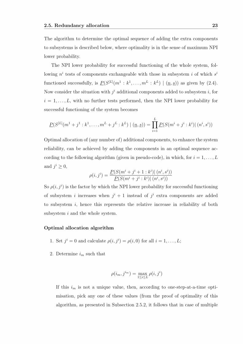
2.5. Redundancy allocation 23
The algorithm to determine the optimal sequence of adding the extra components
to subsystems is described below, where optimality is in the sense of maximum NPI
lower probability.
The NPI lower probability for successful functioning of the whole system, fol-
lowing ni tests of components exchangeable with those in subsystem i of which si
functioned successfully, is P (S[L](m1 : k1, . . . , mL : kL) | (n, s)) as given by (2.4).
Now consider the situation with ji additional components added to subsystem i, for
i = 1, . . . , L, with no further tests performed, then the NPI lower probability for
successful functioning of the system becomes
P (S[L](m1 + j1 : k1, . . . ,mL + jL : kL) | (n, s)) =L∏
i=1
P (S(mi + ji : ki)| (ni, si))
Optimal allocation of (any number of) additional components, to enhance the system
reliability, can be achieved by adding the components in an optimal sequence ac-
cording to the following algorithm (given in pseudo-code), in which, for i = 1, . . . , L
and ji ≥ 0,
ρ(i, ji) =P (S(mi + ji + 1 : ki)| (ni, si))
P (S(mi + ji : ki)| (ni, si))
So ρ(i, ji) is the factor by which the NPI lower probability for successful functioning
of subsystem i increases when ji + 1 instead of ji extra components are added
to subsystem i, hence this represents the relative increase in reliability of both
subsystem i and the whole system.
Optimal allocation algorithm
1. Set ji = 0 and calculate ρ(i, ji) = ρ(i, 0) for all i = 1, . . . , L;
2. Determine im such that
ρ(im, jim) = max1≤i≤L
ρ(i, ji)
If this im is not a unique value, then, according to one-step-at-a-time opti-
misation, pick any one of these values (from the proof of optimality of this
algorithm, as presented in Subsection 2.5.2, it follows that in case of multiple

2.5. Redundancy allocation 24
maxima these can be taken in any order without affecting the optimal lower
probability of system functioning at any stage);
3. Add an extra component to subsystem im: set jim := jim + 1 and calculate
ρ(im, jim);
4. Return to Step 2, using the same values ρ(i, ji) as in the previous step for i 6=
im, together with the new value ρ(im, jim) for subsystem im, as just calculated
in Steps 2 and 3.
This algorithm can be stopped at any time, whatever stop-criterion is defined,
and will always give optimal allocation of extra components. After stopping the
algorithm, the vector j = (j1, . . . , jL) gives the number of extra components added
to each subsystem, and the NPI lower probability for successful functioning of the
system after adding these extra components is equal to
P (S[L](m1 + j1 : k1, . . . ,mL + jL : kL) | (n, s)) =
P (S[L](m1 : k1, . . . , mL : kL) | (n, s)) ×L∏
i=1
ji−1∏li=0
ρ(i, li).
This enables easy calculation of the NPI lower probability following Step 3 of the
above algorithm, as it just requires the previous value of this NPI lower probability
to be multiplied by the ρ(im, jim) calculated at that step.
2.5.2 Optimality of redundancy allocation algorithm
It is claimed that the sequential one-step redundancy allocation algorithm presented
in Section 2.5.1 provides overall optimality in the sense of maximum NPI lower prob-
ability for successful functioning of the system, no matter how many components
can be added in total, or indeed how the number of extra components is deter-
mined. The proof of this optimality is given below with some change of notation for
convenience.
Let ν(n,m) denote the number of equally likely orderings of those variables for
which the data Y n1 = s must be followed by Y n+m
n+1 ≥ k as explained in Section 2.3.1.

2.5. Redundancy allocation 25
Let λ(n,m) = P (m : k | n, s), so
λ(n,m) =
(n + m
n
)−1
ν(n,m) (2.6)
For (n,m) such that n + m ≥ s + k these λ(n,m) are
λ(n,m) =
P (Y n+m
n+1 ≥ k | Y n1 = s), n ≥ s, m ≥ k
1, 0 < n ≤ s − 1,
0, 0 < m ≤ k − 1
.
As ν counts paths the following key equation holds
ν(n,m + 1) = ν(n,m) + ν(n − 1,m + 1), n + m ≥ s + k
and by employing standard binomial identities
(n + m + 1)λ(n,m + 1) = (m + 1)λ(n,m) + nλ(n − 1, m + 1) . (2.7)
When s = 1 and k = 1 the simple form λ(n,m) = m/(n + m) holds for n + m ≥ 1.
It was shown by Coolen-Schrijner et al. [29] that {λ(s,m)}m is increasing and
log-concave, specifically {λ(s,m) : m ≥ k} is increasing in m, {λ(s,m+1)/λ(s,m)) :
m ≥ k} is decreasing in m. To prove that the redundancy allocation algorithm in
the previous section is optimal, these results need to be generalized to the case
of general n. The first step is establishing monotonicity for each n, working with
diagonal sets of nodes, i.e. with n + m fixed.
Lemma 2.1. For any n ≥ s, t ≥ s + k,
1. {λ(t − m,m) : k − 1 ≤ m ≤ t} is increasing in m;
2. {λ(n,m) : m ≥ k − 1} is increasing in m.
Proof.
1. This is true for t = s + k as 0 < s/(s + k) < 1. Suppose it is true for t ≥ s + k
and consider the sequence for t + 1. By (2.7)
λ(t − m, m + 1) =m + 1
t + 1λ(t − m,m) +
t − m
t + 1λ(t − m − 1,m + 1)
> λ(t − m,m) (induc. hyp.) (2.8)
>m
t + 1λ(t + 1 − m,m − 1) +
t + 1 − m
t + 1λ(t − m,m)
= λ(t + 1 − m,m) (by (2.7) )

2.5. Redundancy allocation 26
and the result holds for all t ≥ s + k by induction.
2. By (2.8), for any n ≥ s, λ(n,m + 1) > λ(n,m) for m ≥ k.
Now the ratios λ(n,m+1)/λ(n,m) are considered. It is slightly more convenient
to work with the reciprocals λ(n,m)/λ(n,m+1). Once again working with diagonal
sets of nodes proves to be easiest.
Lemma 2.2. For each t = s + k + 1, s + k + 2, . . . the sequence of ratios
{λ(t − m, m − 1)/λ(t + 1 − m,m) : k ≤ m ≤ t + 1 − s} is increasing in m.
Proof. The case t = s + k + 1 is readily established by direct calculation. Suppose
that the result has been established for some t − 1 where t ≥ s + k + 2. Introduce
the notation `m = λ(t − 1 − m,m), Lm = λ(t − m,m) to simplify the expressions.
Next it is shown that {Lm−1/Lm : m ≥ k} is increasing. Using (2.7)
Lm
Lm+1
=m`m−1 + (t − m)`m
(m + 1)`m + (t − 1 − m)`m+1
,Lm−1
Lm
=(m − 1)`m−2 + (t + 1 − m)`m−1
m`m−1 + (t − m)`m
so (after cross-multiplying) the aim is to show that
L2m − Lm+1Lm−1 > 0 for m = k, k + 1, . . . , t + 1 − s . (2.9)
From the induction hypothesis it follows that ∆2m ≡ `2
m − `m+1`m−1 > 0 for m =
k,. . . , t − s and similarly that for k + 1 ≤ m ≤ t + 1 − s,
Γ1 ≡ `m`m−1 − `m+1`m−2 = `m+1`m−1
(`m
`m+1
− `m−2
`m−1
)> 0
(Γ1 = 0 when m = k since `k−1 = `k−2 = 0). Further from Lemma 2.1
Γ2 ≡ `m`m−2 + `m+1`m−1 − `m+1`m−2 − `m`m+1 = (`m−2 − `m−1)(`m − `m+1) > 0
for k+1 ≤ m ≤ t−s with Γ2 = 0 when m = k or m = t+1−s. For k ≤ m ≤ t+1−s
t2(L2m − Lm+1Lm−1) = m2∆2
m−1 + (t − m)2∆2m +
(m(t − m) − t
)Γ1 + Γ2 > 0
as m(t − m) > t. Thus (2.9) holds and the result for all t ≥ s + k + 1 follows by
induction.
2.5. Redundancy allocation 27
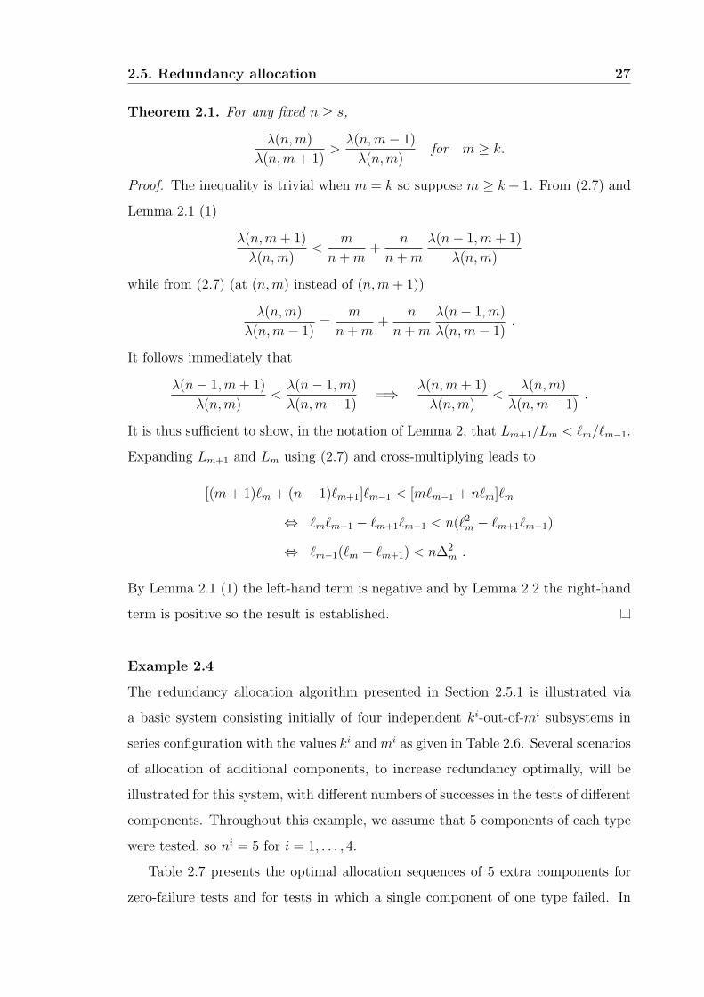
Theorem 2.1. For any fixed n ≥ s,
λ(n,m)
λ(n,m + 1)>
λ(n, m − 1)
λ(n,m)for m ≥ k.
Proof. The inequality is trivial when m = k so suppose m ≥ k + 1. From (2.7) and
Lemma 2.1 (1)
λ(n,m + 1)
λ(n,m)<
m
n + m+
n
n + m
λ(n − 1,m + 1)
λ(n,m)
while from (2.7) (at (n,m) instead of (n,m + 1))
λ(n,m)
λ(n,m − 1)=
m
n + m+
n
n + m
λ(n − 1,m)
λ(n,m − 1).
It follows immediately that
λ(n − 1,m + 1)
λ(n,m)<
λ(n − 1,m)
λ(n,m − 1)=⇒ λ(n,m + 1)
λ(n,m)<
λ(n,m)
λ(n,m − 1).
It is thus sufficient to show, in the notation of Lemma 2, that Lm+1/Lm < `m/`m−1.
Expanding Lm+1 and Lm using (2.7) and cross-multiplying leads to
[(m + 1)`m + (n − 1)`m+1]`m−1 < [m`m−1 + n`m]`m
⇔ `m`m−1 − `m+1`m−1 < n(`2m − `m+1`m−1)
⇔ `m−1(`m − `m+1) < n∆2m .
By Lemma 2.1 (1) the left-hand term is negative and by Lemma 2.2 the right-hand
term is positive so the result is established.
Example 2.4
The redundancy allocation algorithm presented in Section 2.5.1 is illustrated via
a basic system consisting initially of four independent ki-out-of-mi subsystems in
series configuration with the values ki and mi as given in Table 2.6. Several scenarios
of allocation of additional components, to increase redundancy optimally, will be
illustrated for this system, with different numbers of successes in the tests of different
components. Throughout this example, we assume that 5 components of each type
were tested, so ni = 5 for i = 1, . . . , 4.
Table 2.7 presents the optimal allocation sequences of 5 extra components for
zero-failure tests and for tests in which a single component of one type failed. In
2.5. Redundancy allocation 28
i ki mi
1 1 2
2 2 3
3 3 5
4 1 4
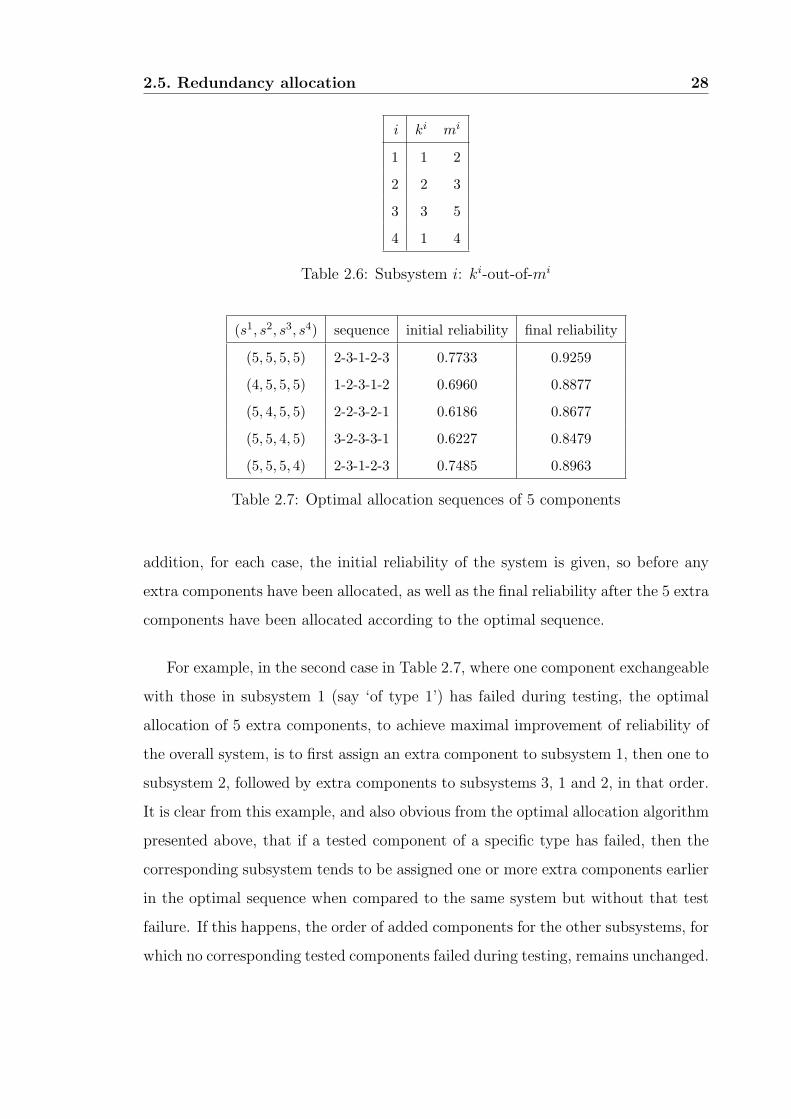
Table 2.6: Subsystem i: ki-out-of-mi
(s1, s2, s3, s4) sequence initial reliability final reliability
(5, 5, 5, 5) 2-3-1-2-3 0.7733 0.9259
(4, 5, 5, 5) 1-2-3-1-2 0.6960 0.8877
(5, 4, 5, 5) 2-2-3-2-1 0.6186 0.8677
(5, 5, 4, 5) 3-2-3-3-1 0.6227 0.8479
(5, 5, 5, 4) 2-3-1-2-3 0.7485 0.8963
Table 2.7: Optimal allocation sequences of 5 components
addition, for each case, the initial reliability of the system is given, so before any
extra components have been allocated, as well as the final reliability after the 5 extra
components have been allocated according to the optimal sequence.
For example, in the second case in Table 2.7, where one component exchangeable
with those in subsystem 1 (say ‘of type 1’) has failed during testing, the optimal
allocation of 5 extra components, to achieve maximal improvement of reliability of
the overall system, is to first assign an extra component to subsystem 1, then one to
subsystem 2, followed by extra components to subsystems 3, 1 and 2, in that order.
It is clear from this example, and also obvious from the optimal allocation algorithm
presented above, that if a tested component of a specific type has failed, then the
corresponding subsystem tends to be assigned one or more extra components earlier
in the optimal sequence when compared to the same system but without that test
failure. If this happens, the order of added components for the other subsystems, for
which no corresponding tested components failed during testing, remains unchanged.
2.6. Redundancy allocation with component costs 29
(s1, s2, s3, s4) sequence initial reliability final reliability
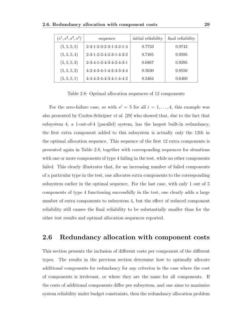
(5, 5, 5, 5) 2-3-1-2-3-2-3-1-3-2-1-4 0.7733 0.9742
(5, 5, 5, 4) 2-3-1-2-3-4-2-3-1-4-3-2 0.7485 0.9595
(5, 5, 5, 3) 2-3-4-1-2-4-3-4-2-4-3-1 0.6867 0.9295
(5, 5, 5, 2) 4-2-4-3-4-1-4-2-4-3-4-4 0.5630 0.8556
(5, 5, 5, 1) 4-4-4-2-4-4-3-4-1-4-4-2 0.3464 0.6460
Table 2.8: Optimal allocation sequences of 12 components
For the zero-failure case, so with si = 5 for all i = 1, . . . , 4, this example was
also presented by Coolen-Schrijner et al. [29] who showed that, due to the fact that
subsystem 4, a 1-out-of-4 (parallel) system, has the largest built-in redundancy,
the first extra component added to this subsystem is actually only the 12th in
the optimal allocation sequence. This sequence of the first 12 extra components is
presented again in Table 2.8, together with corresponding sequences for situations
with one or more components of type 4 failing in the test, while no other components
failed. This clearly illustrates that, for an increasing number of failed components
of a particular type in the test, one allocates extra components to the corresponding
subsystem earlier in the optimal sequence. For the last case, with only 1 out of 5
components of type 4 functioning successfully in the test, one clearly adds a large
number of extra components to subsystem 4, but the effect of reduced component
reliability still causes the final reliability to be substantially smaller than for the
other test results and optimal allocation sequences reported.
2.6 Redundancy allocation with component costs
This section presents the inclusion of different costs per component of the different
types. The results in the previous section determine how to optimally allocate
additional components for redundancy for any criterion in the case where the cost
of components is irrelevant, or where they are the same for all components. If
the costs of additional components differ per subsystem, and one aims to maximize
system reliability under budget constraints, then the redundancy allocation problem

2.6. Redundancy allocation with component costs 30
becomes more complex. This problem can be formulated as follows:
Let ci be the cost to add one extra component to subsystem i. Then the total
cost of these additional components being added to the whole system is:
C(j) = C(j1, . . . , jL) =L∑
i=1
ciji
Obtaining optimal system reliability with a fixed budget B means that we need to
add J additional components to the whole system (J =∑L
i=1 ji) in order to
maximizeL∏
i=1
ji−1∏li=0
ρ(i, li)
subject to the restriction
L∑i=1
ciji 6 B ji ≥ 0 ∀i = 1, . . . , L
This goal function can be replaced by: maximize∑L
i=1
∑ji−1li=0 ln(ρ(i, li)). This prob-
lem is close in nature to the well-known knapsack problems in discrete optimisa-
tion [43]. The knapsack problem is a problem of how to choose items to maximize
their total value under a constraint of maximal weight. Let us assume that we can
choose from items 1, . . . , n with weights a1, a2, . . . , an and profits p1, p2, . . . , pn. The
capacity of the knapsack K ∈ N is also given. The task is now to select a subset
of the items so that its total weight does not exceed K and its profit is maximized
among those subsets. The integer program formulation of the knapsack problem is
the following. For all i = 1, . . . , n we have a variable xi ∈ {0, 1},
maximize∑
pixi
subject to ∑aixi 6 K
There are different versions of the knapsack problem [43], for example the single
knapsack problem is the case where one container (or knapsack) must be filled with
an optimal subset of items. If more than one container is available, the multiple
knapsack problem will be considered. Also, according to the number of copies allo-
cated of each item one can distinguish between the unbounded knapsack problem,

2.6. Redundancy allocation with component costs 31
i ki mi ci
1 3 4 5
2 2 3 4
3 4 6 3
4 2 4 6
Table 2.9: Subsystem i: ki-out-of-mi
which places no bound on the number of each item, and the bounded knapsack
problem, which restricts the number of each item to a maximum value. The typical
formulation in practice is the 0-1 knapsack problem, where only one copy of each
item is available.
The system considered in this chapter consists of series configurations of L inde-
pendent ki-out-of-mi subsystems. For each i = 1, . . . , L, ρ(i, ji) is strictly decreasing
in ji, but ci is assumed to be fixed. It means that the extra components to be al-
located with cost (weight) ci and utility (value) ln ρ(i, li) are not the same. This
allocation problem is considered as a 0-1 knapsack problem, which can be solved by
basic dynamic programming.
Example 2.5
The redundancy allocation under fixed budget B using a knapsack problem for-
mulation is illustrated via a basic system consisting initially of four independent
ki-out-of-mi subsystems in series configuration, with the values ki, mi and ci as
given in Table 2.9. Several scenarios of allocation of additional components, under
different budgets, will be illustrated for this system. Throughout this example, we
assume that 5 components of each type were tested, so ni = 5 for i = 1, . . . , 4. To
concentrate on the effect of the budget B, we assume zero-failure testing, so si = 5
for i = 1, . . . , 4.

2.7. Concluding remarks 32
Budget extra components to final reliability
B each subsystem i
1 2 3 4 total
17 2 1 1 0 4 0.8046
18 1 1 3 0 5 0.8082
19 1 2 2 0 5 0.8151
20 2 1 2 0 5 0.8281
21 2 1 2 0 5 0.8281
22 1 2 3 0 6 0.8284
23 2 1 3 0 6 0.8416
24 2 2 2 0 6 0.8488
Table 2.10: Optimal allocation of the components for different budgets
Table 2.10 presents the optimal allocation of the extra components for budget B
varying from 17 to 24. In addition, for each case, the optimal final reliability after
extra components have been allocated is given, the initial reliability of this system
is 0.6227.
Table 2.10 shows that increasing the budget has different effects on the allocation
of the extra components added to the system. For example, increasing the budget
from 17 to 18 results in increasing the extra components added to subsystem 3 to
3, and reducing the extra components added to subsystem 1 to 1 with one extra
component added to the whole system. However, increasing the budget from 18
to 19 does not increase the total number of extra components added to the whole
system, but it assigns a different number to some subsystems. Increasing the budget
from 20 to 21 has no effect.
2.7 Concluding remarks
Coolen-Schrijner et al. [29] presented the basic application of NPI for Bernoulli
random quantities to inference on reliability of a system which consists of several
ki-out-of-mi subsystems in series configuration. They proved that the NPI model
2.7. Concluding remarks 33
is very tractable, enabling a powerful optimal redundancy allocation algorithm, but
they only derived this result for redundancy allocation following zero-failure testing.
In this chapter, this algorithm is proven to be optimal for redundancy allocation for
such systems following any test results (as long as at least one component of each
type functioned successfully in the tests), which is a powerful result for practical
application of this algorithm.
Redundancy allocation with a fixed budget using the knapsack problem is pre-
sented in this chapter as a first step to inclusion of different costs per component
of the different types. Further steps could involve the opportunity to reduce the
ki of a subsystem, which in practice could e.g. be achieved either by a change to
the demands on the subsystem or by guaranteeing that an installed component will
actually function, this may be possible if components can be analyzed in great de-
tail. Perhaps more important from practical perspective is the generalization with
different losses taken into account, corresponding to failures of different subsystems,
which can be considered as different failure modes. This is important in situations
where such systems have multiple failure modes, and in particular where the losses
incurred by failures due to different failure modes vary substantially. Further aspects
of testing can also be considered, for example time required to test different com-
ponents, with restrictions on overall time available for testing. Also, one needs to
determine how many zero-failure tests are required in order to demonstrate reliabil-
ity. Coolen and Coolen-Schrijner [23] and Rahrouh et al. [47] present related theory
of reliability demonstration from the perspectives of NPI and Bayesian statistics.

Chapter 3
Subsystems consisting of one type
of component
3.1 Introduction
In the previous chapter we have presented nonparametric predictive inference (NPI)
for system reliability, with specific attention to redundancy allocation. Series sys-
tems were considered in which each subsystem i is a ki-out-of-mi system. The
different subsystems were assumed to consist of different types of components, each
type having undergone prior success-failure testing. In this chapter, these results are
generalized by allowing different ki-out-of-mi subsystems to consist of components
of the same type. Such components are exchangeable with regard to the information
about them contained in test results but they play different roles in the system if
they are in different subsystems.
In Section 3.2 NPI lower and upper probabilities for series of ki-out-of-mi subsys-
tems consisting of single-type components are derived by counting paths on the grid,
in a similar way as described in Chapter 2. We start with series of two ki-out-of-mi
subsystems. Then the results are generalized to systems with L > 2 ki-out-of-mi
subsystems. The NPI lower and upper cumulative joint distribution functions for
the event of interest are presented. Examples in Section 3.3 illustrate these NPI
lower and upper probabilities for system functioning. Section 3.4 contains some
concluding remarks.
34

3.2. Series of subsystems consisting of single-type components 35
/ m k / m k / mk1 1 2 2 L L
Figure 3.1: Series of L ki-out-of-mi subsystems consisting of single-type components
3.2 Series of subsystems consisting of single-type
components
Consider a system consisting of a series configuration of L ki-out-of-mi subsystems,
with the subsystems consisting of components of the same type (see Figure 3.1).
Such components are exchangeable with regard to the information about them con-
tained in test results, but they play different roles in the system if they are in
different subsystems. To apply the NPI approach for such a system, n components
that are exchangeable with the m (m = m1 + · · · + mL) components in the system
considered, have to be tested. The event that such a system functions successfully
is denoted by S[L](m1 : k1, · · · ,mL : kL). The aim is to derive the NPI lower and
upper probabilities for the event that the system functions given the test data,
P (S[L](m1 : k1, · · · , mL : kL) | (n, s))
and
P (S[L](m1 : k1, · · · , mL : kL) | (n, s))
respectively.
Before presenting the general results for any number L of subsystems, the case
of a system consisting of L = 2 subsystems is considered in detail.
3.2.1 Two subsystems
Consider a system which consists of a series configuration of two ki-out-of-mi sub-
systems. These subsystems consist of components of the same type (see Figure
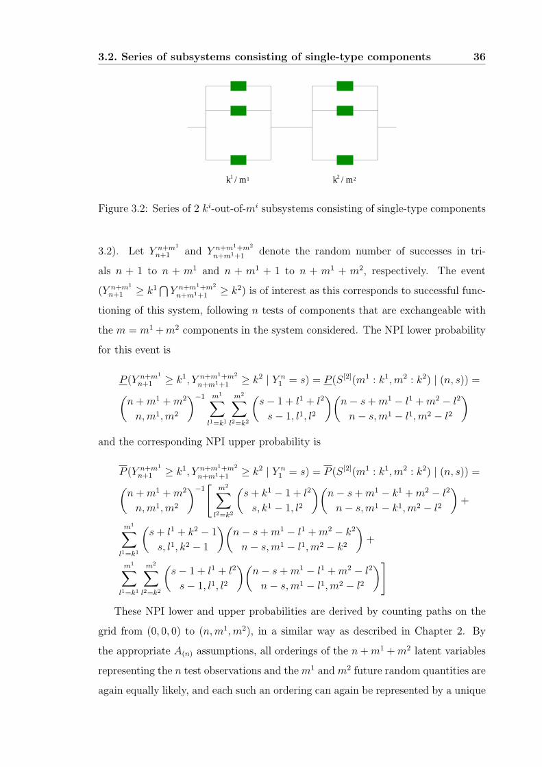
3.2. Series of subsystems consisting of single-type components 36
k / m k / m1 2 2 1
Figure 3.2: Series of 2 ki-out-of-mi subsystems consisting of single-type components
3.2). Let Y n+m1
n+1 and Y n+m1+m2
n+m1+1 denote the random number of successes in tri-
als n + 1 to n + m1 and n + m1 + 1 to n + m1 + m2, respectively. The event
(Y n+m1
n+1 ≥ k1∩
Y n+m1+m2
n+m1+1 ≥ k2) is of interest as this corresponds to successful func-
tioning of this system, following n tests of components that are exchangeable with
the m = m1 + m2 components in the system considered. The NPI lower probability
for this event is
P (Y n+m1
n+1 ≥ k1, Y n+m1+m2
n+m1+1 ≥ k2 | Y n1 = s) = P (S[2](m1 : k1,m2 : k2) | (n, s)) =(
n + m1 + m2
n, m1,m2
)−1 m1∑l1=k1
m2∑l2=k2
(s − 1 + l1 + l2
s − 1, l1, l2
)(n − s + m1 − l1 + m2 − l2
n − s,m1 − l1,m2 − l2
)and the corresponding NPI upper probability is
P (Y n+m1
n+1 ≥ k1, Y n+m1+m2
n+m1+1 ≥ k2 | Y n1 = s) = P (S[2](m1 : k1,m2 : k2) | (n, s)) =(
n + m1 + m2
n, m1,m2
)−1[
m2∑l2=k2
(s + k1 − 1 + l2
s, k1 − 1, l2
)(n − s + m1 − k1 + m2 − l2
n − s,m1 − k1, m2 − l2
)+
m1∑l1=k1
(s + l1 + k2 − 1
s, l1, k2 − 1
)(n − s + m1 − l1 + m2 − k2
n − s,m1 − l1,m2 − k2
)+
m1∑l1=k1
m2∑l2=k2
(s − 1 + l1 + l2
s − 1, l1, l2
)(n − s + m1 − l1 + m2 − l2
n − s,m1 − l1,m2 − l2
)]
These NPI lower and upper probabilities are derived by counting paths on the
grid from (0, 0, 0) to (n,m1,m2), in a similar way as described in Chapter 2. By
the appropriate A(n) assumptions, all orderings of the n + m1 + m2 latent variables
representing the n test observations and the m1 and m2 future random quantities are
again equally likely, and each such an ordering can again be represented by a unique

3.2. Series of subsystems consisting of single-type components 37
1(n,m ,m )2
n
m
m
(0,0,0)s
k
k
1
2
1
2
Figure 3.3: All possible paths from the point (0,0,0) to the point (n,m1,m2)
path from (0, 0, 0) to (n,m1,m2) (see Figure 3.3). The above NPI lower probability
follows by counting all paths which go through (s, r1, r2) for r1 ≥ k1 and r2 ≥ k2
but not through any point (s, r1, r2) with r1 less than k1 or with r2 less than k2.
The corresponding NPI upper probability follows by counting all such paths that go
through at least one point (s, r1, r2) with r1 ≥ k1 and r2 ≥ k2.
3.2.2 L ≥ 2 subsystems
Using similar counting arguments on an L + 1-dimensional grid, the NPI lower and
upper probabilities for successful functioning of the system consisting of a series
configuration of L ≥ 2 ki-out-of-mi subsystems with single-type components, are
P (S[L](m1 : k1, · · · ,mL : kL) | (n, s)) =
(n + m1 + · · · + mL
n,m1, · · · ,mL
)−1
m1∑lL=k1
· · ·mL∑
lL=kL
(s − 1 + l1 + · · · + lL
s − 1, l1, · · · , lL
)(n − s + m1 − l1 + · · · + mL − lL
n − s,m1 − l1, · · · ,mL − lL
)and
P (S[L](m1 : k1, · · · ,mL : kL) | (n, s)) =
(n + m1 · · · + mL
n,m1, · · · ,mL
)−1[
L∑i=1
Ai+
m1∑l1=k1
· · ·mL∑
lL=kL
(s − 1 + l1 + · · · + lL
s − 1, l1, · · · , lL
)(n − s + m1 − l1 + · · · + mL − lL
n − s,m1 − l1, · · · ,mL − lL
)]
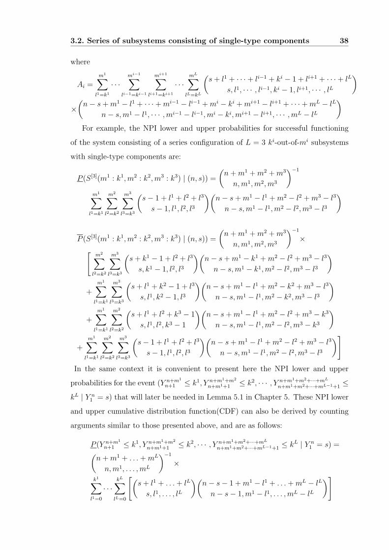
3.2. Series of subsystems consisting of single-type components 38
where
Ai =m1∑
l1=k1
· · ·mi−1∑
li−1=ki−1
mi+1∑li+1=ki+1
· · ·mL∑
lL=kL
(s + l1 + · · · + li−1 + ki − 1 + li+1 + · · · + lL
s, l1, · · · , li−1, ki − 1, li+1, · · · , lL
)×(
n − s + m1 − l1 + · · · + mi−1 − li−1 + mi − ki + mi+1 − li+1 + · · · + mL − lL
n − s,m1 − l1, · · · ,mi−1 − li−1, mi − ki,mi+1 − li+1, · · · ,mL − lL
)For example, the NPI lower and upper probabilities for successful functioning
of the system consisting of a series configuration of L = 3 ki-out-of-mi subsystems
with single-type components are:
P (S[3](m1 : k1,m2 : k2, m3 : k3) | (n, s)) =
(n + m1 + m2 + m3
n,m1, m2,m3
)−1
m1∑l1=k1
m2∑l2=k2
m3∑l3=k3
(s − 1 + l1 + l2 + l3
s − 1, l1, l2, l3
)(n − s + m1 − l1 + m2 − l2 + m3 − l3
n − s,m1 − l1,m2 − l2,m3 − l3
)
P (S[3](m1 : k1,m2 : k2, m3 : k3) | (n, s)) =
(n + m1 + m2 + m3
n,m1, m2,m3
)−1
×[m2∑
l2=k2
m3∑l3=k3
(s + k1 − 1 + l2 + l3
s, k1 − 1, l2, l3
)(n − s + m1 − k1 + m2 − l2 + m3 − l3
n − s,m1 − k1, m2 − l2, m3 − l3
)
+m1∑
l1=k1
m3∑l3=k3
(s + l1 + k2 − 1 + l3
s, l1, k2 − 1, l3
)(n − s + m1 − l1 + m2 − k2 + m3 − l3
n − s,m1 − l1,m2 − k2,m3 − l3
)
+m1∑
l1=k1
m2∑l2=k2
(s + l1 + l2 + k3 − 1
s, l1, l2, k3 − 1
)(n − s + m1 − l1 + m2 − l2 + m3 − k3
n − s,m1 − l1,m2 − l2,m3 − k3
)
+m1∑
l1=k1
m2∑l2=k2
m3∑l3=k3
(s − 1 + l1 + l2 + l3
s − 1, l1, l2, l3
)(n − s + m1 − l1 + m2 − l2 + m3 − l3
n − s,m1 − l1,m2 − l2,m3 − l3
)]In the same context it is convenient to present here the NPI lower and upper
probabilities for the event (Y n+m1
n+1 ≤ k1, Y n+m1+m2
n+m1+1 ≤ k2, · · · , Y n+m1+m2+···+mL
n+m1+m2+···+mL−1+1≤
kL | Y n1 = s) that will later be needed in Lemma 5.1 in Chapter 5. These NPI lower
and upper cumulative distribution function(CDF) can also be derived by counting
arguments similar to those presented above, and are as follows:
P (Y n+m1
n+1 ≤ k1, Y n+m1+m2
n+m1+1 ≤ k2, · · · , Y n+m1+m2+···+mL
n+m1+m2+···+mL−1+1≤ kL | Y n
1 = s) =(n + m1 + . . . + mL
n,m1, . . . , mL
)−1
×
k1∑l1=0
· · ·kL∑
lL=0
[(s + l1 + . . . + lL
s, l1, . . . , lL
)(n − s − 1 + m1 − l1 + . . . + mL − lL
n − s − 1,m1 − l1, . . . , mL − lL
)]

3.3. Examples 39
Figure 3.4: The Dutch Oosterscheldekering (source: earth.google.com)
and
P (Y n+m1
n+1 ≤ k1, Y n+m1+m2
n+m1+1 ≤ k2, · · · , Y n+m1+m2+···+mL
n+m1+m2+···+mL−1+1≤ kL | Y n
1 = s) =(n + m1 + . . . + mL
n,m1, . . . , mL
)−1
×
k1∑l1=0
· · ·kL∑
lL=0
[(s − 1 + l1 + . . . + lL
s − 1, l1, . . . , lL
)(n − s + m1 − l1 + . . . + mL − lL
n − s, m1 − l1, . . . , mL − lL
)]
The above NPI lower CDF follows by counting all paths which go through any pair
(s, r1, r2) and (s+1, r1, r2) respectively for r1 ≤ k1 and r2 ≤ k2. The corresponding
NPI upper CDF probability follows by counting all such paths that go through any
point (s, r1, r2) with r1 ≤ k1 and r2 ≤ k2.
3.3 Examples
In this section the NPI lower and upper probabilities for successful functioning of
the system considered in this chapter are illustrated via three related examples. Al-
though these examples are purely illustrative for the presented theory, the numbers
chosen are inspired by the Dutch Oosterscheldekering (Eastern Scheldt storm surge
barrier), which is part of the Delta works series of dams to protect the Netherlands

3.3. Examples 40
k = 58 k = 59 k = 60 k = 61 k = 62
n s P P P P P P P P P P
1 1 0.079 1 0.063 1 0.048 1 0.032 1 0.016 1
2 2 0.151 1 0.122 1 0.092 1 0.062 1 0.031 1
3 3 0.217 1 0.176 1 0.134 1 0.091 1 0.046 1
2 0.021 0.217 0.014 0.176 0.008 0.134 0.004 0.091 0.001 0.046
5 5 0.330 1 0.272 1 0.211 1 0.145 1 0.075 1
4 0.060 0.330 0.041 0.272 0.025 0.211 0.013 0.145 0.005 0.075
10 10 0.538 1 0.458 1 0.367 1 0.260 1 0.139 1
9 0.192 0.538 0.139 0.458 0.090 0.367 0.049 0.260 0.018 0.139
8 0.051 0.192 0.032 0.139 0.017 0.090 0.007 0.049 0.002 0.018
7 0.011 0.051 0.006 0.032 0.003 0.017 0.001 0.007 0.000 0.002
20 20 0.763 1 0.681 1 0.573 1 0.431 1 0.244 1
30 30 0.868 1 0.800 1 0.699 1 0.548 1 0.326 1
40 40 0.922 1 0.867 1 0.780 1 0.633 1 0.392 1
50 50 0.952 1 0.910 1 0.834 1 0.696 1 0.446 1
60 60 0.969 1 0.936 1 0.872 1 0.744 1 0.492 1
62 62 0.971 1 0.941 1 0.878 1 0.752 1 0.500 1
100 100 0.993 1 0.980 1 0.946 1 0.855 1 0.617 1
Table 3.1: NPI lower and upper probabilities for a k-out-of-62 system
from flooding [18]. The Oosterscheldekering consists of three sections, with 15 steel
doors in the northern section, 16 in the middle section, and 31 in the southern
section (see Figure 3.4). The NPI lower and upper probabilities for successful func-
tioning of the system in these examples could be interpreted as those for successful
functioning of this barrier on a single application, following test results of n doors.
Of course, this assumes exchangeability of the functioning of the individual doors,
which may not be deemed to be an appropriate assumption. In Example 3.1 we start
with a single k-out-of-62 system. In Examples 3.2 and 3.3 we regard this system as
consisting of two or three ki-out-of-mi systems.

3.3. Examples 41
Example 3.1
In this example we suppose that the barrier consists of 62 steel doors next to each
other in one line. Table 3.1 presents the NPI lower and upper probabilities for a k-
out-of-62 system, with k varying from 58 to 62, on the basis of tests of n components
that are exchangeable with the 62 components in the system, and s components in
the tests functioning successfully.
If tests have revealed no failures, so s = n, then the NPI upper probability
of system functioning is equal to 1, which reflects that such tests do not contain
evidence against the possibility that such components would always function. The
corresponding lower probabilities in these cases are increasing in the number of tests,
if the tests did not reveal any failures, which reflects the increasing evidence in favour
of at least k components out of 62 functioning in the system. With relatively few
tests performed, and many of the 62 components in the system required to function,
the effect of a failure in the tests on the predicted system reliability is substantial.
This example illustrates that P (S(m : k)| (n, s)) = P (S(m : k)| (n, s + 1)), which
generally holds for these NPI lower and upper probabilities [29]. It is worth noticing
the lower probability P (S(62 : 62)| (62, 62)) = 0.5, which is actually precisely 1/2
and is the same as would be derived if the whole 62-out-of-62 system were instead
considered to be a single unit, and if one exchangeable unit (hence also such a
system) had been tested and had been successful, as P (S(1 : 1)| (1, 1)) = 0.5. Table
3.1 shows that the lower and upper probabilities are decreasing in k when keeping m
and n constant, and increasing in n when keeping m and k constant. This is most
obvious from the large differences between the values at the top left and bottom
right of Table 3.1.
Example 3.2
As we mentioned before, the Oosterscheldekering consists of three sections, with 15
steel doors in the northern section, 16 in the middle section, and 31 in the southern
section. Suppose now that the functioning of the barrier requires specific numbers
of doors in each section to function. The assumption of exchangeability of the doors
remains with regard to the uncertainty of their functioning and the way in which

3.3. Examples 42
k1 = k2 = 29 k1 = 29, k2 = 30 k1 = k2 = 30 k1 = k2 = 31
n s P P P P P P P P
1 1 0.066 1 0.050 1 0.040 1 0.016 1
2 2 0.126 1 0.096 1 0.077 1 0.031 1
3 3 0.182 1 0.139 1 0.113 1 0.046 1
2 0.015 0.182 0.010 0.139 0.006 0.113 0.001 0.046
5 5 0.280 1 0.218 1 0.178 1 0.075 1
4 0.045 0.280 0.028 0.218 0.019 0.178 0.005 0.075
10 10 0.467 1 0.375 1 0.314 1 0.139 1
9 0.148 0.467 0.099 0.375 0.070 0.314 0.018 0.139
8 0.036 0.148 0.020 0.099 0.012 0.070 0.002 0.018
7 0.007 0.036 0.003 0.020 0.002 0.012 0.000 0.002
20 20 0.687 1 0.579 1 0.503 1 0.244 1
30 30 0.803 1 0.701 1 0.625 1 0.326 1
40 40 0.868 1 0.778 1 0.708 1 0.392 1
50 50 0.908 1 0.829 1 0.766 1 0.446 1
60 60 0.934 1 0.865 1 0.809 1 0.492 1
62 62 0.938 1 0.871 1 0.816 1 0.500 1
100 100 0.977 1 0.936 1 0.901 1 0.617 1
Table 3.2: NPI lower and upper probabilities with m1 = m2 = 31
we learn from test data on similar doors. For the functioning of the system it is
important to distinguish the doors according to which section they are in. In this
example, suppose that the northern and middle sections can be combined to one k1-
out-of-31 subsystem, with the southern section a separate k2-out-of-31 subsystem,
and these two subsystems form together the overall system in series configuration.
Some NPI lower and upper probabilities for functioning of the whole system are
presented in Table 3.2.
Comparing Tables 3.1 and 3.2, it is clear that the lower and upper probabilities
in the final columns, where the system only functions if all components function, are
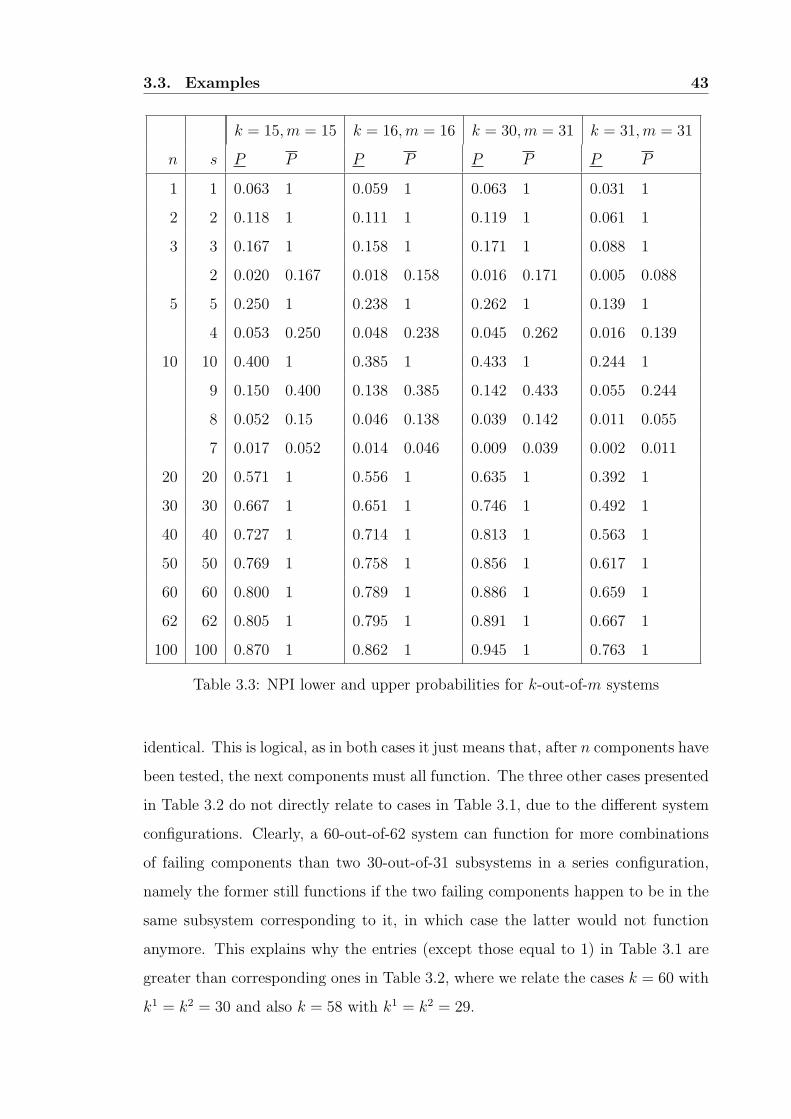
3.3. Examples 43
k = 15,m = 15 k = 16,m = 16 k = 30, m = 31 k = 31,m = 31
n s P P P P P P P P
1 1 0.063 1 0.059 1 0.063 1 0.031 1
2 2 0.118 1 0.111 1 0.119 1 0.061 1
3 3 0.167 1 0.158 1 0.171 1 0.088 1
2 0.020 0.167 0.018 0.158 0.016 0.171 0.005 0.088
5 5 0.250 1 0.238 1 0.262 1 0.139 1
4 0.053 0.250 0.048 0.238 0.045 0.262 0.016 0.139
10 10 0.400 1 0.385 1 0.433 1 0.244 1
9 0.150 0.400 0.138 0.385 0.142 0.433 0.055 0.244
8 0.052 0.15 0.046 0.138 0.039 0.142 0.011 0.055
7 0.017 0.052 0.014 0.046 0.009 0.039 0.002 0.011
20 20 0.571 1 0.556 1 0.635 1 0.392 1
30 30 0.667 1 0.651 1 0.746 1 0.492 1
40 40 0.727 1 0.714 1 0.813 1 0.563 1
50 50 0.769 1 0.758 1 0.856 1 0.617 1
60 60 0.800 1 0.789 1 0.886 1 0.659 1
62 62 0.805 1 0.795 1 0.891 1 0.667 1
100 100 0.870 1 0.862 1 0.945 1 0.763 1
Table 3.3: NPI lower and upper probabilities for k-out-of-m systems
identical. This is logical, as in both cases it just means that, after n components have
been tested, the next components must all function. The three other cases presented
in Table 3.2 do not directly relate to cases in Table 3.1, due to the different system
configurations. Clearly, a 60-out-of-62 system can function for more combinations
of failing components than two 30-out-of-31 subsystems in a series configuration,
namely the former still functions if the two failing components happen to be in the
same subsystem corresponding to it, in which case the latter would not function
anymore. This explains why the entries (except those equal to 1) in Table 3.1 are
greater than corresponding ones in Table 3.2, where we relate the cases k = 60 with
k1 = k2 = 30 and also k = 58 with k1 = k2 = 29.

3.3. Examples 44
(k1, k2, k3) : (14, 15, 30) (15, 16, 30) (15, 16, 31)
n s P P P P P P
1 1 0.045 1 0.024 1 0.016 1
2 2 0.087 1 0.047 1 0.031 1
3 3 0.127 1 0.069 1 0.046 1
2 0.008 0.127 0.003 0.069 0.001 0.046
5 5 0.197 1 0.110 1 0.075 1
4 0.024 0.197 0.009 0.110 0.005 0.075
10 10 0.345 1 0.200 1 0.139 1
9 0.085 0.345 0.033 0.200 0.018 0.139
8 0.016 0.085 0.005 0.033 0.002 0.018
7 0.003 0.016 0.001 0.005 0.000 0.002
20 20 0.542 1 0.337 1 0.244 1
30 30 0.664 1 0.437 1 0.326 1
40 40 0.744 1 0.513 1 0.392 1
50 50 0.799 1 0.571 1 0.446 1
60 60 0.838 1 0.618 1 0.492 1
62 62 0.844 1 0.626 1 0.500 1
100 100 0.919 1 0.736 1 0.617 1
Table 3.4: NPI lower and upper probabilities with m1 = 15,m2 = 16,m3 = 31
Example 3.3
Let us now consider the system of 62 components split up into three subsystems,
with m1 = 15, m2 = 16 and m3 = 31 components, inspired by the three sections of
the Oosterscheldekering. First, let us consider the reliability of each of these three
subsystems independently of each other, so we consider each as a single k-out-of-m
system. The NPI lower and upper probabilities for successful functioning of each
of these systems individually, based on s successfully functioning components in n
tests, are given in Table 3.3, for the values k and m as indicated in the columns.
3.3. Examples 45
These NPI lower and upper probabilities give an indication of the reliability
of the individual subsystems considered, when considering them independently of
the other systems. It is crucial, however, that in the application in this example,
these subsystems consist of the same type of component, for which only limited
test information is available. Hence, if it were known that one of these subsystems
functions satisfactorily, let us assume this would be the subsystem with m = 15
and assuming that this would function only if k = 15, then for the next subsystem
considered we are more confident in the reliability of the components, as now in
addition to the test results for the n tested components it is known that a further
15 components all function satisfactorily. This has a substantial impact on overall
reliability when we combine the subsystems into a single system.
If one were to neglect the interdependence of the components in the different
subsystems, one would make the mistake of quantifying the system’s reliability by
multiplying the NPI lower and upper probabilities of successful functioning of the
subsystems, as mentioned in Chapter 2 for independent subsystems. For example,
consider the third column of Table 3.2, involving a series system with two 30-out-of-
31 subsystems on the basis of s components functioning well out of n components
tested. If we would, instead, multiply the lower and upper probabilities for two
individual 30-out-of-31 systems, based on the same test information, so effectively
we would take the squared values of the entries in the third column in Table 3.3, then
the latter would lead to substantially smaller values for the lower probability, and
also for the upper probability for all cases where this is not equal to one. To illustrate
this important issue, assume that n = 10 components had been tested, of which s = 9
functioned successfully. The corresponding NPI lower and upper probabilities for
successful functioning of the series system with two 30-out-of-31 subsystems (Table
3.2, third column) are 0.070 and 0.314, respectively. If one would, mistakenly,
neglect the interdependence of these two subsystems, which use components of the
same type, and multiply the NPI lower and upper probabilities for the individual
30-out-of-31 subsystems (Table 3.3, third column), this would lead to the values
0.1422 = 0.020 for the lower and 0.4332 = 0.187 for the upper probability, which are
substantially smaller than the correct values.
3.3. Examples 46
Let us now consider the 62-component system as consisting of three subsystems
in series structure, with m1 = 15, m2 = 16 and m3 = 31 components. Table 3.4
presents NPI lower and upper probabilities for some situations reflecting satisfactory
functioning of the whole system depending on the specific numbers ki (i = 1, 2, 3)
of components required to function per subsystem.
Again, if all 62 components need to function (ki = mi for all i), then the NPI
lower and upper probabilities are as in Tables 3.1 and 3.2 for the same situation.
Suppose that the whole system functions satisfactorily if in each subsystem not more
than one component fails, leading to the NPI lower and upper probabilities in the
first column of Table 3.4. If we had not separated the two smallest subsystems,
so instead had assumed that the whole system consisted of two subsystems with
m1 = m2 = 31, as considered in Example 3.2 with corresponding NPI lower and
upper probabilities given in Table 3.2, and if we had allowed two failing components
for the first subsystem with m1 = 31 components, then (see column 2 in Table 3.2)
the NPI lower and upper probabilities (the latter if different from 1) would have been
larger than those with the three subsystems taken into account separately. This is
due to the fact that there would be more combinations of the failing components
included in the counts for the lower and upper probabilities in Table 3.2, namely
those with two failing components in one, and zero in the other, of the individual
subsystems with 15 and 16 components. This illustrates clearly that one must
carefully define the requirements on the subsystems in order for the overall system
to function, which is of course directly linked to the appropriate system structure.
Examples 3.1, 3.2 and 3.3 clearly show the effect of increasing numbers of tests on
the system reliability. If all n components tested succeeded in their task, so s = n,
then the NPI lower probabilities increase as function of n, but the rate of increase
decreases. This is in line with intuition as it reflects that, with all tests being
successful, the positive effect of a further successful test on the lower probability
of system functioning decreases with increasing n. This can also be used to set a
minimum number of tests, assuming no failures will be discovered, in order to meet a
reliability requirement formulated as a minimum value for the NPI lower probability
of system functioning. This is relevant in high-reliability testing, where failures in
3.4. Concluding remarks 47
tests typically lead to redesign of the units followed by a new stage of testing, and
hence one needs to determine how many zero-failure tests are required in order to
demonstrate reliability. Coolen and Coolen-Schrijner [23] and Rahrouh et al. [47]
present related theory of reliability demonstration from the perspectives of NPI and
Bayesian statistics.
3.4 Concluding remarks
This chapter presented an important step in the development of NPI for more com-
plex system structures, as components of one type frequently occur in different
subsystems. As a first step for this research, we have generalized NPI for Bernoulli
quantities [12] to distinguish between subgroups of the m future observations, and
we have derived lower and upper probabilities which quantify the reliability of such
systems. A further important step will be presented in the next chapter namely NPI
for reliability of voting systems with multiple component types.
In Chapter 2 an optimal algorithm was presented for redundancy allocation
related to the NPI approach to reliability of systems consisting of independent ki-
out-of-mi subsystems, each consisting of a single type of component, which are
different for different subsystems. The algorithm was proven to be optimal, and this
algorithm is straightforward to implement and requires negligible computing time.
This algorithm will be a basis for constructing an algorithm for a more general system
in Chapter 4. Numerical examples indicate that a similarly attractive algorithm will
again be optimal for the system in this chapter, but we have not managed to prove
this as a general property.
Chapter 4
Voting systems with multiple
component types
4.1 Introduction
It has been generally acknowledged that redundancy in systems leads to increased
reliability. However, during the last decade there has been increasing debate about
the value of redundancy, in particular highlighting the effect of common-cause fail-
ures or other kinds of dependent failures, where multiple components fail at the
same time or in a small period of time, see for example Pate-Cornell et al. [46]
and Hoepfer et al. [37]. It is typically argued that, whilst additional components in
parallel system structures provide redundancy and increase system reliability, their
positive effect may be restricted due to common-cause failures which possibly af-
fect all components of a particular type. Whilst such common-cause failures can
be taken into account [55], a natural solution lies in the combination of redundancy
and diversity, so the use of components of different types, leaving the system less
severely affected by possible common-cause failures. This basic idea also has ap-
plications to reliability of software-based systems, where redundancy with diversity
can for example be achieved for a safety protection system by using multiple diverse
channels performing the same function [41].
In this chapter, we restrict terminology to the basic situation of simple voting
systems, so k-out-of-m systems in which at least k components must function in
48

4.1. Introduction 49
order for the system to function, and with the system consisting of components
which all perform the same function. One can think for example about batteries
or smoke detectors as components in a system. We now consider the possibility
that the components are of different types, for example batteries or smoke detectors
from different manufacturers, and that our information about the reliability of the
components results from tests performed on such components.
We do not consider common-cause failures, but we focus on a perhaps even
more important reason for aiming at diversity of components, which appears to
have received little attention in the literature, namely the lack of perfect knowledge
about the reliability of the components. This limited information about component
reliability causes the random functioning of multiple components of one type in
a system to be mutually dependent in the sense that functioning or not of one
component in the system would change our total information on components of this
type sufficiently to affect our beliefs on reliability of another component of this type
in the system. As shown by Coolen-Schrijner et al. [29], this may well result in
higher risk than may be expected without careful consideration of the uncertainties
involved.
However, a possibly more important reason for diversity is illustrated here,
namely the lack of perfect knowledge about the reliability of the components.
The system considered in this chapter is presented in Section 4.2. Subsection
4.2.1 provides a brief description of the system. In Subsection 4.2.2 the NPI lower
and upper probabilities for functioning of a voting system with any number of com-
ponent types are presented. The derivation of these NPI lower and upper probabil-
ities is presented in Subsection 4.2.3. The optimal allocation of extra components
is discussed in subsection 4.2.4. Section 4.3 presents examples to illustrate these
lower and upper probabilities and to discuss some specific related features including
diversity. Section 4.4 contains some concluding remarks.

4.2. Multiple component types 50
k / m
Figure 4.1: Voting systems with multiple component types
4.2 Multiple component types
4.2.1 System description
Consider a single voting system consisting of different types of components. They
are assumed to perform the same function within the system, but the test infor-
mation differs per type of component. Throughout this chapter we assume that
functioning of components of different types is fully independent, in the sense that
any information on functioning of components of one type does not hold any infor-
mation about functioning of components of another type. Suppose that there are T
types of components and the voting system consists of mt components of type t for
each t = 1, . . . , T , so m = m1 + . . . + mT components in total (see Figure 4.1).
This system functions if and only if at least k of its m components function,
whatever their types. To apply the NPI approach for the reliability of this system,
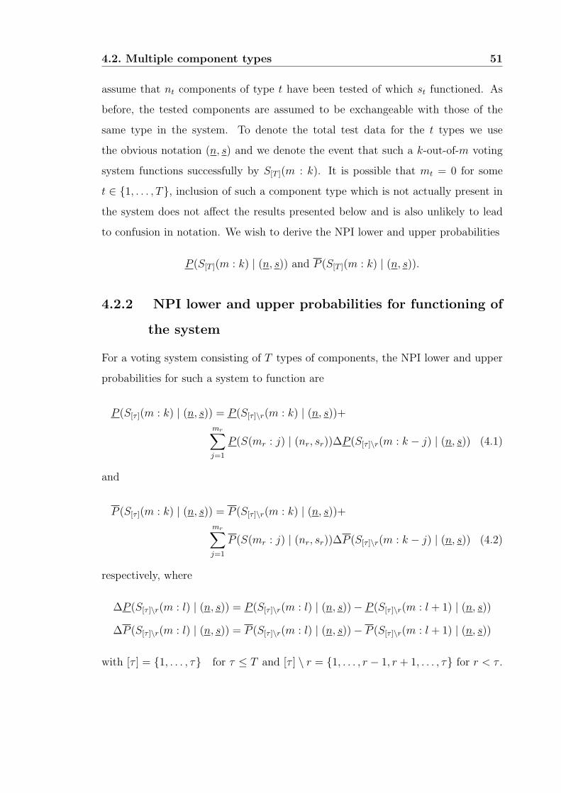
4.2. Multiple component types 51
assume that nt components of type t have been tested of which st functioned. As
before, the tested components are assumed to be exchangeable with those of the
same type in the system. To denote the total test data for the t types we use
the obvious notation (n, s) and we denote the event that such a k-out-of-m voting
system functions successfully by S[T ](m : k). It is possible that mt = 0 for some
t ∈ {1, . . . , T}, inclusion of such a component type which is not actually present in
the system does not affect the results presented below and is also unlikely to lead
to confusion in notation. We wish to derive the NPI lower and upper probabilities
P (S[T ](m : k) | (n, s)) and P (S[T ](m : k) | (n, s)).
4.2.2 NPI lower and upper probabilities for functioning of
the system
For a voting system consisting of T types of components, the NPI lower and upper
probabilities for such a system to function are
P (S[τ ](m : k) | (n, s)) = P (S[τ ]\r(m : k) | (n, s))+
mr∑j=1
P (S(mr : j) | (nr, sr))∆P (S[τ ]\r(m : k − j) | (n, s)) (4.1)
and
P (S[τ ](m : k) | (n, s)) = P (S[τ ]\r(m : k) | (n, s))+
mr∑j=1
P (S(mr : j) | (nr, sr))∆P (S[τ ]\r(m : k − j) | (n, s)) (4.2)
respectively, where
∆P (S[τ ]\r(m : l) | (n, s)) = P (S[τ ]\r(m : l) | (n, s)) − P (S[τ ]\r(m : l + 1) | (n, s))
∆P (S[τ ]\r(m : l) | (n, s)) = P (S[τ ]\r(m : l) | (n, s)) − P (S[τ ]\r(m : l + 1) | (n, s))
with [τ ] = {1, . . . , τ} for τ ≤ T and [τ ] \ r = {1, . . . , r − 1, r + 1, . . . , τ} for r < τ .
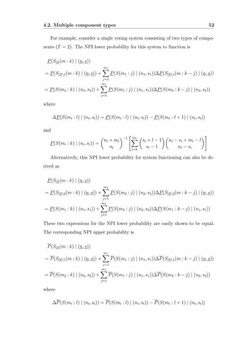
4.2. Multiple component types 52
For example, consider a single voting system consisting of two types of compo-
nents (T = 2). The NPI lower probability for this system to function is
P (S[2](m : k) | (n, s))
= P (S[2]\1(m : k) | (n, s)) +
m1∑j=1
P (S(m1 : j) | (n1, s1))∆P (S[2]\1(m : k − j) | (n, s))
= P (S(m2 : k) | (n2, s2)) +
m1∑j=1
P (S(m1 : j) | (n1, s1))∆P (S(m2 : k − j) | (n2, s2))
where
∆P (S(mt : l) | (nt, st)) = P (S(mt : l) | (nt, st)) − P (S(mt : l + 1) | (nt, st))
and
P (S(mt : k) | (nt, st)) =
(nt + mt
nt
)−1[
mt∑l=k
(st + l − 1
st − 1
)(nt − st + mt − l
nt − st
)]Alternatively, this NPI lower probability for system functioning can also be de-
rived as
P (S[2](m : k) | (n, s))
= P (S[2]\2(m : k) | (n, s)) +
m2∑j=1
P (S(m2 : j) | (n2, s2))∆P (S[2]\2(m : k − j) | (n, s))
= P (S(m1 : k) | (n1, s1)) +
m2∑j=1
P (S(m2 : j) | (n2, s2))∆P (S(m1 : k − j) | (n1, s1))
These two expressions for the NPI lower probability are easily shown to be equal.
The corresponding NPI upper probability is
P (S[2](m : k) | (n, s))
= P (S[2]\1(m : k) | (n, s)) +
m1∑j=1
P (S(m1 : j) | (n1, s1))∆P (S[2]\1(m : k − j) | (n, s))
= P (S(m2 : k) | (n2, s2)) +
m1∑j=1
P (S(m1 : j) | (n1, s1))∆P (S(m2 : k − j) | (n2, s2))
where
∆P (S(mt : l) | (nt, st)) = P (S(mt : l) | (nt, st)) − P (S(mt : l + 1) | (nt, st))

4.2. Multiple component types 53
and
P (S(mt : k) | (nt, st)) =
(nt + mt
nt
)−1 [(st + k
st
)(nt − st + mt − k
nt − st
)+
mt∑l=k+1
(st + l − 1
st − 1
)(nt − st + mt − l
nt − st
)]and it can also be derived as
P (S[2](m : k) | (n, s))
= P (S[2]\2(m : k) | (n, s)) +
m2∑j=1
P (S(m2 : j) | (n2, s2))∆P (S[2]\2(m : k − j) | (n, s))
= P (S(m1 : k) | (n1, s1)) +
m2∑j=1
P (S(m2 : j) | (n2, s2))∆P (S(m1 : k − j) | (n1, s1))
In the next subsection the derivation of these NPI lower and upper probabilities will
be presented in detail.
4.2.3 Derivation of the NPI lower and upper probabilities
for functioning of the system
The NPI lower and upper probabilities (4.1) and (4.2) are derived by considering all
combinations representing successful functioning of the system, using the theorem of
total probability for classical probabilities as shown in Lemma 4.1 (below) for general
T . The key aspect is that the theorem of total probability is used for all precise
probability distributions in the NPI-based structure M (as discussed in Section 1.1),
and that sharp lower and upper bounds are derived.
Before we proceed, we introduce further notation. Let Xt denote the number of
the mt components of type t which function and write
ct (j) = P (Xt ≥ j), ut (j) = P (Xt ≥ j), `t (j) = P (Xt ≥ j).
Furthermore, for any set S ⊂ {1, . . . , T}, let
cS(j) = P(∑
t∈S Xt ≥ j), ∆ct(j) = ct(j) − ct(j + 1)
and ∆cS(j) = cS(j) − cS(j + 1)
with boundary conditions:
ct(j) = cS(j) = 1 for j ≤ 0,

4.2. Multiple component types 54
ct(j) = 0 for j > mt,
cS(j) = 0 for j >∑
t∈S mt,
∆ct(j) = ∆cS(j) = 0 for j < 0.
The notation stated above for classical probabilities c is also used below for upper
and lower probabilities, replacing c by u or l, respectively.
Lemma 4.1. Suppose X1, . . . , XT , with Xt ∈ {0, 1, . . . , mt} for t ∈ {1, . . . , T}, are
independent random quantities. For each τ ∈ {2, . . . , T} and 1 ≤ r < τ ,
u[τ ](k) = u[τ ]\r(k) +mr∑j=1
ur(j)∆u[τ ]\r(k − j) (4.3)
`[τ ](k) = `[τ ]\r(k) +mr∑j=1
`r(j)∆`[τ ]\r(k − j) (4.4)
Proof. We provide the proof for upper probabilities, the proof for lower probabilities
is identical with u replaced by ` everywhere. We present the argument for T = 2
types of components first and then generalize to T > 2. For T = 2, X1 and X2 are
independent so
P (X1 + X2 ≥ k) =
m1∑j=0
P (X1 = j)P (X2 ≥ k − j) (4.5)
and, using the introduced notation, this gives
c[2](k) =
m1∑j=0
∆c1 (j) c2 (k − j) 6m1∑j=0
∆c1 (j) u2 (k − j)
as each ∆c1 (j) ≥ 0. Also
m1∑j=0
∆c1 (j) u2 (k − j) = c1 (0) u2 (k) +
m1∑j=1
c1 (j) ∆u2 (k − j)
6 u1 (0) u2 (k) +
m1∑j=1
u1 (j) ∆u2 (k − j)
as each ∆u2 (k − j) ≥ 0, so
c[2](k) 6 u1 (0) u2 (k) +
m1∑j=1
u1 (j) ∆u2 (k − j) . (4.6)
As equality in (4.6) is actually possible with c2 (j) = u2 (j) and c1 (j) = u1 (j) for
each j, the upper probability u[2](k), which is the minimum upper bound for c[2](k),
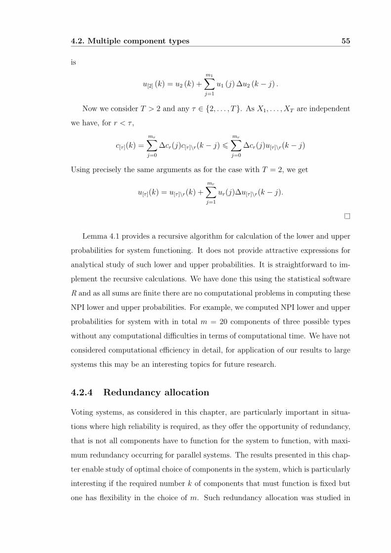
4.2. Multiple component types 55
is
u[2] (k) = u2 (k) +
m1∑j=1
u1 (j) ∆u2 (k − j) .
Now we consider T > 2 and any τ ∈ {2, . . . , T}. As X1, . . . , XT are independent
we have, for r < τ ,
c[τ ](k) =mr∑j=0
∆cr(j)c[τ ]\r(k − j) 6mr∑j=0
∆cr(j)u[τ ]\r(k − j)
Using precisely the same arguments as for the case with T = 2, we get
u[τ ](k) = u[τ ]\r(k) +mr∑j=1
ur(j)∆u[τ ]\r(k − j).
Lemma 4.1 provides a recursive algorithm for calculation of the lower and upper
probabilities for system functioning. It does not provide attractive expressions for
analytical study of such lower and upper probabilities. It is straightforward to im-
plement the recursive calculations. We have done this using the statistical software
R and as all sums are finite there are no computational problems in computing these
NPI lower and upper probabilities. For example, we computed NPI lower and upper
probabilities for system with in total m = 20 components of three possible types
without any computational difficulties in terms of computational time. We have not
considered computational efficiency in detail, for application of our results to large
systems this may be an interesting topics for future research.
4.2.4 Redundancy allocation
Voting systems, as considered in this chapter, are particularly important in situa-
tions where high reliability is required, as they offer the opportunity of redundancy,
that is not all components have to function for the system to function, with maxi-
mum redundancy occurring for parallel systems. The results presented in this chap-
ter enable study of optimal choice of components in the system, which is particularly
interesting if the required number k of components that must function is fixed but
one has flexibility in the choice of m. Such redundancy allocation was studied in

4.2. Multiple component types 56
Chapter 2 for systems consisting of voting subsystems, where each subsystem has
a single type of components which are different from those in other subsystems. It
is also of interest to study optimal redundancy allocation for voting systems with
different types of components as presented here. While no general optimality re-
sults have been proven yet, there is a strong feeling that making sequentially the
optimal choices for adding single components leads to the overall optimal allocation
of multiple extra components. This is in line with the results in Chapter 2, and
all numerical examples studied suggest that it also holds for the systems considered
here.
For the special case of parallel systems, so with k = 1 and mt components of
type t (t = 1, . . . , T ), optimal allocation of extra components is straightforward if
one aims at maximum NPI lower probability for the event that the system functions.
This lower probability is
P (ST (m : 1) | (n, s)) = 1 −T∏
t=1
mt∏jt=1
nt − st + jt
nt + jt
where the product term on the right-hand side is the NPI upper probability for
the event that the parallel system does not function, which occurs if and only if all
its components fail. Adding one more component of type t0 leads to decrease of
this upper probability by a factornt0−st0+mt0+1
nt0+mt0+1, so it is optimal to assign one more
component of the type for which this factor is minimal, and the simple product
form of this upper probability implies that optimal allocation of multiple extra
components can be achieved by optimal sequential allocation of single components.
Actually, if one would allow a large enough number of extra components in such
a parallel system, then eventually one would add one or more components of each
type, even if test results for one type were very poor compared to the other types
(assuming, as we do throughout this chapter, that there is at least one successfully
functioning component of each type in the test). Suppose that type t0 ∈ {1, . . . , T}
has led to the poorest test results (lowest ratio st/nt) and that there are already
mt0 components of this type in the system. Then t0 is still the best component
type to add to the system once there are already mt components of type t, for each
t ∈ {1, . . . , T}, t 6= t0, with mt > (nt0 +mt0 + 1)(st/st0)−nt − 1. This result follows
4.3. Examples 57
straightforwardly from the above argument on sequential minimisation of the upper
probability for the event that the parallel system does not function, and is illustrated
in Example 4.3 in Section 4.3. We have not achieved a proof of a similar result for
other voting systems, but numerical results suggest that it holds for all such systems
with fixed value of k if m can be increased.
4.3 Examples
In this section we illustrate the NPI lower and upper probabilities presented in
Subsection 4.2.2. In Example 4.1 we focus on the optimal choice of the number of
components of each type in a k-out-of-20 system with 2 types of components, with
optimality in the sense of maximum NPI lower probability of system functioning. It
is natural to consider the lower probability for reliability inferences, as it reflects the
strength of the evidence in favour of the system’s reliability, and as such could be
interpreted as a conservative inference. In Example 4.2 we consider a system with
3 types of components. Example 4.3 includes a brief discussion of the important
topics of redundancy and diversity.
Example 4.1
Consider a voting system with in total m = 20 components of two possible types,
of which at least k must function in order for the system to function. Table 4.1
presents the optimal choices of m1 and m2, the numbers of components of each
type, for several test histories of components of types 1 and 2. All possible values
for k ranging from 1 (parallel system) to 20 (series system) are considered. The
notation (x, y)p is used to indicate that all permutations of x, y are optimal.
If only one component of each type has been tested, and both functioned well,
then it is optimal to use 10 components of each type if k ≤ 10, but for k > 10 it is
optimal to use only one type of component. This is a direct consequence of the way
in which the interdependence of the reliability of individual components of one type
is taken into account. Let us consider the two extreme cases with k = 1 and k = 20.
For k = 1 with test history (nt, st) = (1, 1) for t = 1, 2, the lower probability for the
first component of type 1 in the system to function is 1/2. If this first component
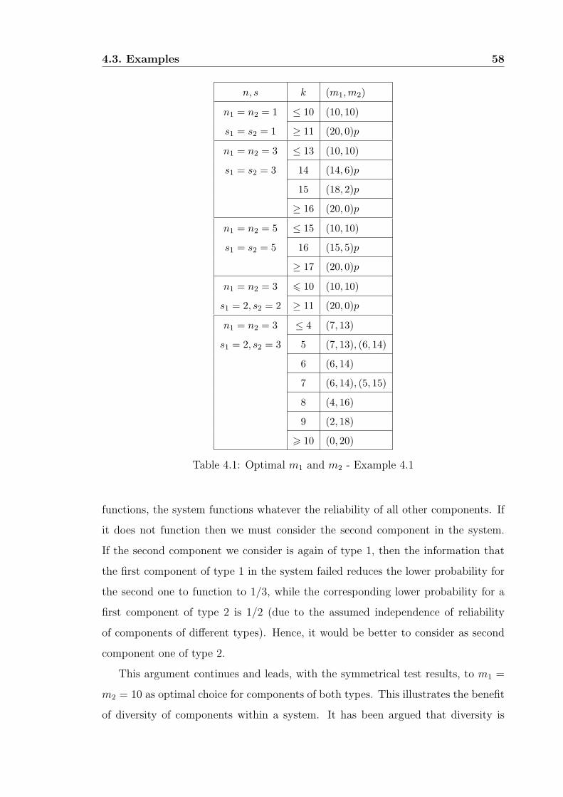
4.3. Examples 58
n, s k (m1,m2)
n1 = n2 = 1 ≤ 10 (10, 10)
s1 = s2 = 1 ≥ 11 (20, 0)p
n1 = n2 = 3 ≤ 13 (10, 10)
s1 = s2 = 3 14 (14, 6)p
15 (18, 2)p
≥ 16 (20, 0)p
n1 = n2 = 5 ≤ 15 (10, 10)
s1 = s2 = 5 16 (15, 5)p
≥ 17 (20, 0)p
n1 = n2 = 3 6 10 (10, 10)
s1 = 2, s2 = 2 ≥ 11 (20, 0)p
n1 = n2 = 3 ≤ 4 (7, 13)
s1 = 2, s2 = 3 5 (7, 13), (6, 14)
6 (6, 14)
7 (6, 14), (5, 15)
8 (4, 16)
9 (2, 18)
> 10 (0, 20)
Table 4.1: Optimal m1 and m2 - Example 4.1
functions, the system functions whatever the reliability of all other components. If
it does not function then we must consider the second component in the system.
If the second component we consider is again of type 1, then the information that
the first component of type 1 in the system failed reduces the lower probability for
the second one to function to 1/3, while the corresponding lower probability for a
first component of type 2 is 1/2 (due to the assumed independence of reliability
of components of different types). Hence, it would be better to consider as second
component one of type 2.
This argument continues and leads, with the symmetrical test results, to m1 =
m2 = 10 as optimal choice for components of both types. This illustrates the benefit
of diversity of components within a system. It has been argued that diversity is
4.3. Examples 59
important to prevent the possible effect of common-cause failures for components of
one type, which is of course true but is not addressed in this chapter. However, a
possibly more important reason for diversity is illustrated here, namely the lack of
perfect knowledge about the reliability of the components.
For a series system all k = 20 components must function. Hence, if the first one
considered is of type 1 and does not function, we do not need to look further as the
system would not function whatever the reliability of all other 19 components. If the
first component (of type 1) functions then it is better for the second component also
to be of type 1 as now it will have lower probability 2/3 to function, based on the test
result and the information we now have on the first component of type 1, compared
to lower probability 1/2 for a component of type 2. This argument now extends to
all 20 components, leading to the optimal series system consisting of components
of a single type. In fact, this argument holds for all series systems, not only those
with symmetric test information. As illustrated by the last case in Table 4.1, if
components of one type performed better in the test than components of the other
type then the optimal choice is to use all components of the type which performed
best in the test. The last case in Table 4.1, in which testing 3 components of type
1 led to one failure with no failures in testing of 3 components of type 2, shows
that one would still include components of type 1 in the ‘more parallel’ systems
considered (k ≤ 9). Again, this is logical from the perspective of diversity.
Table 4.1 further shows that the transition, when considered as function of k, of
the optimal (m1, m2) from them being equal to the other extreme with one being
equal to 20 and the other equal to 0, does not occur immediately in all situations.
For example, if 3 components of each type were tested and no failures had been
observed, then m1 = m2 = 10 is optimal for all k ≤ 13, and for k ≥ 16 it is optimal
to only use components of one type in the system. However, for k = 14 or 15 it is
optimal to use different positive values for m1 and m2.
Example 4.2
This example considers a voting system with in total m = 6 components of three
different types. The optimal choices of m1, m2 and m3, and the corresponding

4.3. Examples 60
k (m1,m2,m3) P
1 (2, 2, 2) 0.995
2 (2, 2, 2) 0.968
A 3 (2, 2, 2) 0.870
4 (2, 2, 2) 0.667
5 (6, 0, 0)p 0.464
6 (6, 0, 0)p 0.250
1 (3, 3, 0) 0.990
2 (3, 3, 0) 0.950
B 3 (3, 3, 0) 0.850
4 (4, 2, 0),(2, 4, 0) 0.656
5 (6, 0, 0),(0, 6, 0) 0.464
6 (6, 0, 0),(0, 6, 0) 0.250
1 (3, 0, 3) 0.982
2 (3, 0, 3),(4, 0, 2) 0.914
C 3 (5, 0, 1),(6, 0, 0) 0.786
4 (6, 0, 0) 0.643
5 (6, 0, 0) 0.464
6 (6, 0, 0) 0.250
Table 4.2: Optimal (m1,m2,m3) and NPI lower probability - Example 4.2
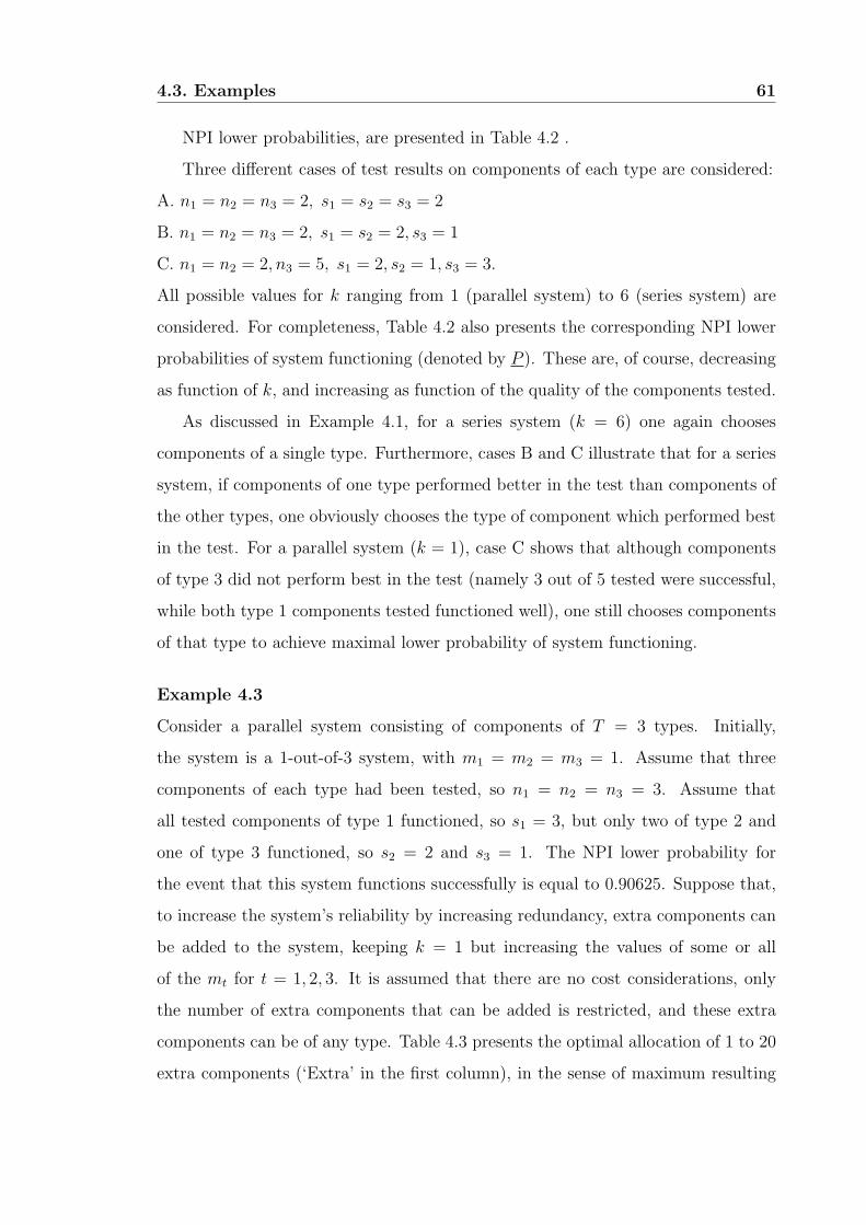
4.3. Examples 61
NPI lower probabilities, are presented in Table 4.2 .
Three different cases of test results on components of each type are considered:
A. n1 = n2 = n3 = 2, s1 = s2 = s3 = 2
B. n1 = n2 = n3 = 2, s1 = s2 = 2, s3 = 1
C. n1 = n2 = 2, n3 = 5, s1 = 2, s2 = 1, s3 = 3.
All possible values for k ranging from 1 (parallel system) to 6 (series system) are
considered. For completeness, Table 4.2 also presents the corresponding NPI lower
probabilities of system functioning (denoted by P ). These are, of course, decreasing
as function of k, and increasing as function of the quality of the components tested.
As discussed in Example 4.1, for a series system (k = 6) one again chooses
components of a single type. Furthermore, cases B and C illustrate that for a series
system, if components of one type performed better in the test than components of
the other types, one obviously chooses the type of component which performed best
in the test. For a parallel system (k = 1), case C shows that although components
of type 3 did not perform best in the test (namely 3 out of 5 tested were successful,
while both type 1 components tested functioned well), one still chooses components
of that type to achieve maximal lower probability of system functioning.
Example 4.3
Consider a parallel system consisting of components of T = 3 types. Initially,
the system is a 1-out-of-3 system, with m1 = m2 = m3 = 1. Assume that three
components of each type had been tested, so n1 = n2 = n3 = 3. Assume that
all tested components of type 1 functioned, so s1 = 3, but only two of type 2 and
one of type 3 functioned, so s2 = 2 and s3 = 1. The NPI lower probability for
the event that this system functions successfully is equal to 0.90625. Suppose that,
to increase the system’s reliability by increasing redundancy, extra components can
be added to the system, keeping k = 1 but increasing the values of some or all
of the mt for t = 1, 2, 3. It is assumed that there are no cost considerations, only
the number of extra components that can be added is restricted, and these extra
components can be of any type. Table 4.3 presents the optimal allocation of 1 to 20
extra components (‘Extra’ in the first column), in the sense of maximum resulting
4.3. Examples 62
Extra (m1,m2,m3) P
0 (1,1,1) 0.90625
1 (2,1,1) 0.96250
2 (3,1,1) 0.98125
3 (4,1,1) 0.98925
4 (4,2,1) 0.99357
5 (5,2,1) 0.99598
6 (6,2,1) 0.99732
7 (6,3,1) 0.99821
8 (7,3,1) 0.99875
9 (7,4,1) 0.99912
10 (8,4,1) 0.99935
11 (9,4,1) 0.99951
12 (9,5,1) 0.99963
13 (10,5,1) 0.99972
14 (10,6,1) 0.99978
15 (10,7,1) 0.99983
16 (11,7,1) 0.99986
17 (12,7,1) 0.99989
18 (12,7,2) 0.99991
19 (13,7,2) 0.99993
20 (13,8,2) 0.99994
Table 4.3: Optimal allocation of extra components from Example 4.3. The red
entries are used to indicate the type of extra component chosen at the specific stage.

4.3. Examples 63
NPI lower probability for the event that the system functions (denoted by P in the
last column).
If one extra component is allowed, it is optimal to add a component of type
1. This is fully as expected, since type A components seem to be more reliable
than type 2 and type 3 components based on the test results. If two further extra
components are allowed, all three would be chosen of type 1. However, if four extra
components are allowed, it is optimal to take the fourth one to be of type 2. For up
to 17 extra components they are all either of type 1 or 2 as presented in Table 4.3.
If an eighteenth extra component is allowed, then it would be optimal to choose a
component of type 3. This illustrates the result presented at the end of Subsection
4.2.3, in particular that it is better to add a component of type 3 than of type 1
if m1 > 11, and better to add a component of type 3 than of type 2 if m2 > 6, so
indeed once m1 ≥ 12 and m2 ≥ 7 the first extra component of type 3 is chosen.
This illustrates an important aspect of NPI for system reliability. NPI takes
explicitly into account that the reliabilities of components of one type in the system
are statistically dependent, as a result of the limited information from the test data.
Effectively, if one has the system with already 3 extra components added in the
optimal manner, it has become quite a reliable system. If, however, this system
does not function, it implies that the components of type 1 seem to be less reliable
than had been expected based on the test results. Hence, at this point a component
of type 2 would seem more reliable, based on the test results and the three assumedly
failing extra components of type 1 in the system. This effect continues similarly,
with each additional component the overall system reliability of course increases but
the consideration of which further extra component to add is based on the situation
where all current system components fail, as that is the only scenario for a parallel
system not to function.
This example illustrates that diversity in redundancy allocation can result di-
rectly from maximisation of reliability, and is due to the limited knowledge about
the reliability of the components of different types. This is an important reason
for diversity that is different to the usually mentioned possibility of common-cause
failures which would lead to all components of one type to fail. This example also

4.4. Concluding remarks 64
illustrates that sequential one-step-at-a-time optimisation leads to the same opti-
mal allocation of extra components as overall optimisation. For parallel systems
as considered here, this result was easily shown to hold as discussed at the end of
Subsection 4.2.4.
4.4 Concluding remarks
This chapter presents another important step in the development of NPI for system
reliability as, due to the use of lower and upper probabilities, it is non-trivial to
deal with multiple component types in a single voting system. The natural next
step is consideration of systems in series structure where each subsystem is a voting
system with multiple types of components and with components of the same type
appearing in different subsystems. This is the main topic of Chapter 5.
In Subsection 4.2.4 we briefly formulated a conjecture on redundancy allocation,
in line with the results in Chapter 2. The basic idea of optimally allocating one more
component, if one can increase m by one without changing k, is pretty straightfor-
ward, as one would just calculate the NPI lower probabilities corresponding to the
possibility to add a component for each of the T component types, and then choose
the type leading to maximum improvement. However, if one can allocate more than
one component, it is not clear that one can proceed with such one-step-at-a-time
optimisation, which would lead to a simple algorithm. We strongly feel that such
an algorithm would be optimal, as was the case for the more basic scenarios we
considered before, but we have not yet achieved a mathematical proof of optimality
for systems with k ≥ 2, for parallel systems (k = 1) the result follows easily as
discussed in Subsection 4.2.4, along the same lines as briefly explained in Section
2.5. A further research challenge is optimal redundancy allocation under cost con-
straints. We believe that for quite a large variety of cost structures the resulting
problems can be formulated as standard optimisation problems, but this is left as a
topic for future research.
The main lesson of this chapter is that considering diversity of components in a
system is important to achieve maximum system reliability in situations with limited
4.4. Concluding remarks 65
information about component reliability, but the optimal configuration depends on
the actual system structure, with diversity generally most useful for parallel systems,
while for series systems one would not opt for diversity and only use components
of the type that gave the best test results. We have only shown this for the simple
systems considered in this chapter, but we strongly feel that similar conclusions will
hold for more general system structures when NPI lower probabilities are used to
express system reliability. Of course, if one feels that there may be common-cause
failures that could simultaneously affect all components of one type in a system,
as suggested as the main reason in favour of diversity in the literature (see Section
4.1), then diversity can have a positive effect on the system reliability which has
not been considered in this chapter. In the NPI framework, common-cause failures
can be considered, although one would require explicit test data on such failures in
order to include it. One may also wish to consider different failure modes, Maturi et
al. [44] recently presented NPI for competing risks data but did not explicitly link
this to system reliability.
Finally, we wish to emphasize that the general idea to use diversity to optimize
performance of a system in situations with uncertainty of performance of the sys-
tem’s components, as presented in this chapter with regard to reliability of voting
systems, is common in many different areas of decision making under uncertainty.
For example, decision makers in finance typically create diverse portfolios of invest-
ments due to uncertainty about performance of individual options, which is close in
nature to the reason for diversity advocated in this chapter.

Chapter 5
Subsystems with multiple
component types
5.1 Introduction
This chapter presents a generalization of results introduced in the previous three
chapters by considering systems with a series structure, where each subsystem is
a voting system with multiple types of components and with components of the
same type appearing in different subsystems. As an example of systems where
such a structure can occur one can think about anti-virus software for computer
networks under possible global attack, with each computer system protected by
a number of anti-virus programmes, some used at multiple computers with some
further programmes possibly just used locally. The functioning of such programmes
may be exchangeable but not ‘identical’ due to local aspects of the computers, for
example how the software has been integrated into the system. Also, one may have
tested the software for a variety of viruses, enabling a judgement of exchangeability
on its performance against a further virus as long as one can assume that this virus
was not created explicitly to circumvent specific anti-virus software.
Section 5.2 provides a brief description of the systems considered in this chapter.
In Section 5.3 the NPI lower and upper probabilities for functioning of a system
consisting of 2 subsystems with 2 component types are presented. In Section 5.4 the
main results of this chapter are presented, namely the NPI lower and upper proba-
66
5.2. Subsystems with multiple component types 67
bilities for functioning of systems with a series structure where each subsystem is a
voting system with multiple types of components. These results generalize the re-
sults in the previous chapters, and hence are the main results presented in this thesis.
Section 5.5 presents examples to illustrate these lower and upper probabilities, and
to discuss some specific related features including aspects of redundancy and diver-
sity. Section 5.6 concludes the chapter with some remarks on further development
of NPI for system reliability and related research challenges.
5.2 Subsystems with multiple component types
Consider a system consisting of L subsystems in a series configuration (see Figure
5.1). Each subsystem is a single voting system consisting of different types of com-
ponents, which are assumed to perform the same function within the subsystem,
but the test information differs per type of component. The important contribu-
tion of this chapter is that different subsystems can contain components of the same
types. This is non-trivial, as the random quantities representing whether these com-
ponents in the system function or not, are not independent in the NPI approach,
given the test results. It is important that this dependence is explicitly taken into
account, in particular when there is relatively little information from tests. Assume
that functioning of components of different types is fully independent, in the sense
that any information on functioning of components of one type does not hold any
information about functioning of components of another type. Suppose that there
are T types of components and the voting subsystem l (l = 1, . . . , L) consists of mlt
components of type t for each t = 1, . . . , T , so ml = ml1 + . . . + ml
T and the whole
system contains in total m1 + . . . + mL components. So, subsystem l functions if
and only if at least kl of its ml components function, whatever their types, and the
entire system functions if and only if all its L subsystems function.
To apply the NPI approach for the reliability of this system, assume that nt
components of type t have been tested, and st of these functioned. As before, the
tested components are assumed to be exchangeable with those of the same type in
the system. To denote the total test data for the t types the vector notation (n, s)

5.2. Subsystems with multiple component types 68
k / mk / m / m1 1 k2 2 L L
Figure 5.1: Subsystems with multiple component types
is used, and we use the obvious notation S[L][T ](m
1 : k1, · · · ,mL : kL) to denote the
event that such a system functions successfully. It is possible that mlt = 0 for some
t ∈ {1, . . . , T} and l ∈ {1, . . . , L}, inclusion of such a component type which is
not actually present in the system does not affect the results presented below and is
unlikely to lead to confusion in notation. Let X lt ∈ {0, 1, . . . ,ml
t} denote the number
out of the mlt components of type t which function in subsystem l, for l ∈ {1, . . . , L}
and t ∈ {1, . . . , T}. The aim is to derive the NPI lower and upper probabilities for
the event that the system functions given the test data,
P (S[L][T ](m
1 : k1, · · · ,mL : kL) | (n, s)) (5.1)
and
P (S[L][T ](m
1 : k1, · · · ,mL : kL) | (n, s)) (5.2)
respectively.
Before presenting the general results for any number L of subsystems and T of
component types, the case of a system consisting of L = 2 subsystems with each
subsystem consisting of the same T = 2 types of components is considered in detail.
5.3. 2 subsystems with 2 component types 69
5.3 2 subsystems with 2 component types
Consider a system consisting of 2 subsystems with 2 component types. The NPI
lower probability for the event that such a system functions is
P (S[2][2](m
1 : k1,m2 : k2) | (n, s)) =
m12∑
i1=0
m22∑
i2=0
[D(X1
2 = i1, X22 = i2 | n2, s2) × P (S
[2][1](m
11 : k1 − i1,m2
1 : k2 − i2 | n1, s1))]
where
D(X12 = i1, X2
2 = i2 | n2, s2) =
P (X12 ≤ i1, X2
2 ≤ i2 | n2, s2) − P (X12 ≤ i1 − 1, X2
2 ≤ i2 | n2, s2)
−P (X12 ≤ i1, X2
2 ≤ i2 − 1 | n2, s2) + P (X12 ≤ i1 − 1, X2
2 ≤ i2 − 1 | n2, s2)
This NPI lower probability is derived by considering all combinations of numbers
and types of components for the two subsystems according to which the system
functions successfully, using the theorem of total probability for precise probabil-
ities as shown in Theorem 5.1 below for general values of L and T . The func-
tion D ensures that maximum possible weight (where ‘maximum’ is over all precise
probability distributions in the NPI-based structure M (see Chapter 1) is given
to lower probabilities P (S[2][1](m
11 : k1 − i1,m2
1 : k2 − i2 | n1, s1)) with small values
of i1 and i2, and as this lower probability is increasing in i1 and i2 this construc-
tion ensures that this P (S[2][2](m
1 : k1,m2 : k2) is the NPI lower probability for
the event that this system functions. This function D is such that it assigns the
maximum possible probability mass, according to the NPI structure, to the event
(X12 = 0, X2
2 = 0), so D(X12 = 0, X2
2 = 0 | n2, s2) = P (X12 = 0, X2
2 = 0 | n2, s2).
Then, D(X12 = 1, X2
2 = 0 | n2, s2) is defined by putting the maximum possible
remaining probability mass from the total probability mass available for the event
(X12 ≤ 1, X2
2 = 0), according to the NPI structure, to the event (X12 = 1, X2
2 = 0).
This is achieved by D(X12 = 1, X2
2 = 0 | n2, s2) = P (X12 ≤ 1, X2
2 = 0 | n2, s2) −
P (X12 = 0, X2
2 = 0 | n2, s2). Following similar reasoning, the maximum possible
remaining probability mass D(X12 = 0, X2
2 = 1 | n2, s2) = P (X12 = 0, X2
2 ≤ 1 |
n2, s2)−P (X12 = 0, X2
2 = 0 | n2, s2) is assigned to the event (X12 = 0, X2
2 = 1). This

5.4. L subsystems with T component types 70
argument is continued, by assigning for increasing i1 and i2 the maximum possible
remaining probability mass D(X12 = i1, X2
2 = i2 | n2, s2). By this construction,
the resulting D is actually a precise probability distribution within the NPI-based
structure for the random quantities (X12 , X
22 ). The use of the NPI lower probabili-
ties P (S[2][1](m
11 : k1 − i1,m2
1 : k2 − i2 | n1, s1)) to achieve the NPI lower probability
P (S[2][2](m
1 : k1,m2 : k2) | (n, s)) is straightforwardly seen to result from minimisation
over the corresponding NPI-based structure for the random quantities (X11 , X
21 ).
In the following section, this assignment of maximum remaining probability
masses will be extended to the general case with L ≥ 2 subsystems and T ≥ 2
types of components in Theorem 5.1, the main ideas are the same as for this case
with L = 2 and T = 2. The NPI lower and upper probabilities needed to calculate
P (S[2][2](m
1 : k1,m2 : k2) | (n, s)) each involve only a single type of component, and
hence are as presented in Chapter 3.
The corresponding NPI upper probability for such a system to function is
P (S[2][2](m
1 : k1,m2 : k2) | (n, s)) =
m12∑
i1=0
m22∑
i2=0
[D(X1
2 = i1, X22 = i2 | n2, s2) × P (S
[2][1](m
11 : k1 − i1,m2
1 : k2 − i2 | n1, s1))]
where
D(X12 = i1, X2
2 = i2 | n2, s2) =
P (X12 ≤ i1, X2
2 ≤ i2 | n2, s2) − P (X12 ≤ i1 − 1, X2
2 ≤ i2 | n2, s2)
−P (X12 ≤ i1, X2
2 ≤ i2 − 1 | n2, s2) + P (X12 ≤ i1 − 1, X2
2 ≤ i2 − 1 | n2, s2)
Justification of this result is similar to that for the NPI lower probability given
above, with the obvious exchange of lower and upper probabilities.
5.4 L subsystems with T component types
For a system consisting of L subsystems with T component types, the NPI lower
and upper probabilities for the system to function are

5.4. L subsystems with T component types 71
P (S[L][τ ] (m
1 :k1, · · · ,mL : kL) | (n, s)) =
m1τ∑
i1=0
· · ·mL
τ∑iL=0
[Dτ (X
1τ = i1, . . . , XL
τ = iL | nτ , sτ )×
P (S[L][τ−1](m
1 : k1 − i1, · · · ,mL : kL − iL) | (n, s))]
(5.3)
and
P (S[L][τ ] (m
1 :k1, · · · ,mL : kL) | (n, s)) =
m1τ∑
i1=0
· · ·mL
τ∑iL=0
[Dτ (X
1τ = i1, . . . , XL
τ = iL | nτ , sτ )×
P (S[L][τ−1](m
1 : k1 − i1, · · · ,mL : kL − iL) | (n, s))]
(5.4)
respectively, with [τ ] = {1, . . . , τ} for τ ≤ T .
To derive the NPI lower and upper probabilities (5.3) and (5.4) for general L
and T we introduce the following notation:
uLt
(i1, i2, . . . , iL
)= P (X1
t ≥ i1, X2t ≥ i2, . . . , XL
t ≥ iL | nt, st)
`Lt
(i1, i2, . . . , iL
)= P (X1
t ≥ i1, X2t ≥ i2, . . . , XL
t ≥ iL | nt, st)
cLt
(i1, i2, . . . , iL
)= P (X1
t ≥ i1, X2t ≥ i2, . . . , XL
t ≥ iL)
eLt
(i1, i2, . . . , iL
)= P (X1
t = i1, X2t = i2, . . . , XL
t = iL)
Furthermore, for any set S ⊂ {1, . . . , T}, let
uLS
(i1, i2, . . . , iL
)= P
(∑t∈S
X1t ≥ i1,
∑t∈S
X2t ≥ i2, . . . ,
∑t∈S
XLt ≥ iL | (n, s)
)
`LS
(i1, i2, . . . , iL
)= P
(∑t∈S
X1t ≥ i1,
∑t∈S
X2t ≥ i2, . . . ,
∑t∈S
XLt ≥ iL | (n, s)
)
cLS
(i1, i2, . . . , iL
)= P
(∑t∈S
X1t ≥ i1,
∑t∈S
X2t ≥ i2, . . . ,
∑t∈S
XLt ≥ iL
)
eLS
(i1, i2, . . . , iL
)= P
(∑t∈S
X1t = i1,
∑t∈S
X2t = i2, . . . ,
∑t∈S
XLt = iL
)
and let [τ ] = {1, . . . , τ} for τ ≤ T .
5.4. L subsystems with T component types 72
The lower and upper probabilities introduced above and used in Theorem 5.1 are
explicitly assumed to be resulting from NPI, as emphasized by inclusion of the test
data in the notation. Of course, of the data (n, s) for all T types of components, only
the (nt, st) with t ∈ S are relevant for uLS and `L
S . The main result of this chapter
is presented in Theorem 5.1, and is a recursive relation that enables calculation
of the NPI lower and upper probabilities for the event that a system of the kind
considered in this chapter functions, given component test data. The main idea is
that, with T different types of components in the system, at each stage (which is one
application of the results of Theorem 5.1) one type of component is separated from
the others and the theorem of total probability is used for the precise probabilities
in the NPI-based structures to take all their possible values into account, leaving
one fewer type of component to be dealt with at the next stage. The complexity of
computations at each stage is based on the number of subsystems L, and the number
of stages is based on the number of component types T . This explains why for large
values of T and L, computational difficulties (in terms of computational time) are
expected to appear. Theorem 5.1 presents the mathematical argument for one such
a stage, with the notational simplification of assuming that the component types to
be considered are the set [τ ], of which the components of type τ are separated from
the others at the stage considered, hence leaving the components of types [τ − 1] to
be considered at the next stage. This can be done without loss of generality, as the
specific types of the components are just labels that can be ordered in any way. An
interesting topic for future research is the effect of specific orders on computational
efficiency. For example it could be best to label the component types 1, . . . , τ , for
any τ ∈ {1, . . . , T}, in such an order that components of one of these types which
appear in the largest number of subsystems are separated from the other component
types first, hence are defined as being of type τ .
Before Theorem 5.1 can be presented, one more concept is required, namely the
generalization of the functions D and D, presented in Section 5.3 for the case L = 2,
for application to systems with more than two subsystems. For components of type
t ∈ {1, . . . , T} and L subsystems, let the function Dt(X1t = i1, . . . , XL
t = iL | nt, st)
be the maximum possible remaining probability mass, corresponding to the NPI

5.4. L subsystems with T component types 73
structure, that can be assigned to the point (i1, . . . , iL) but not to any other point
(a1, . . . , aL) with integers al ∈ {0, . . . , il}. Hence, for L = 2 the function D2(X12 =
i1, X22 = i2 | n2, s2) is equal to the function D discussed above. Generally, this means
that Dt(X1t = 0, . . . , XL
t = 0 | nt, st) = P (X1t = 0, . . . , XL
t = 0 | nt, st), with further
values derived as combinations of these upper cumulative joint distribution function
values at (i1, . . . , iL) and at such points (a1, . . . , aL) with integers al ∈ {0, . . . , il},
ensuring that no probability mass is included more than once. For ease of notation,
let
g(i1, i2, · · · , iL) = P (X1t ≤ i1, X2
t ≤ i2, · · · , XLt ≤ iL | nt, st)
g(i1−1, i2−1, · · · , iL−1) = P (X1t ≤ i1−1, X2
t ≤ i2−1, · · · , XLt ≤ iL−1 | nt, st)
gj1(i1, · · · , ij1−1, ij1 − 1, ij1+1, · · · , iL) =
P (X1t ≤ i1, · · · , Xj1
t ≤ ij1 − 1, Xj1+1t ≤ ij1+1, · · · , XL
t ≤ iL | nt, st)
gj1,··· ,jh(i1, · · · , ij1−1, ij1 − 1, · · · , ijh − 1, ijh+1, · · · , iL) =
P (X1t ≤ i1, · · · , Xj1
t ≤ ij1−1, · · · , Xjht ≤ ijh−1, Xjh+1
t ≤ ijh+1, · · · , XLt ≤ iL | nt, st)
where
1 ≤ j1 < j2 < · · · < jh ≤ L
and
P (X1t ≤ i1, X2
t ≤ i2, · · · , XLt ≤ iL | nt, st) =
i1∑y1=0
· · ·iL∑
yL=0
Dt(X1t = y1, X2
t = y2, · · · , XLt = yL | nt, st)
5.4. L subsystems with T component types 74
Using the notation introduced above and the inclusion-exclusion principle, we get
i1∑y1=0
· · ·iL∑
yL=0
Dt(X1t = y1, X2
t = y2, · · · , XLt = yL | nt, st) =
Dt(X1t = i1, X2
t = i2, · · · , XLt = iL | nt, st) +
[L∑
j1=1
gj1(i1, · · · , ij1 − 1, ij1+1, · · · , iL)
−∑
j1,j2 : 1≤j1<j2≤L
gj1,j2(i1, · · · , ij1 − 1, ij2 − 1, ij2+1, · · · , iL)
+∑
j1,j2,j3 : 1≤j1<j2<j3≤L
gj1,j2,j3(i1, · · · , ij1 − 1, ij2 − 1, ij3 − 1, ij3+1, · · · , iL)
− · · · + (−1)L−1 g(i1 − 1, i2 − 1, · · · , iL − 1)]
so
Dt(X1t = i1, X2
t = i2, · · · , XLt = iL | nt, st) =
g(i1, i2, · · · , iL) −
[L∑
j1=1
gj1(i1, · · · , ij1 − 1, ij1+1, · · · , iL)
−∑
j1,j2 : 1≤j1<j2≤L
gj1,j2(i1, · · · , ij1 − 1, ij2 − 1, ij2+1, · · · , iL)
+∑
j1,j2,j3 : 1≤j1<j2<j3≤L
gj1,j2,j3(i1, · · · , ij1 − 1, ij2 − 1, ij3 − 1, ij3+1, · · · , iL)
− · · · + (−1)L−1 g(i1 − 1, i2 − 1, · · · , iL − 1)]
The NPI upper cumulative joint distribution functions involved follow directly from
the results in Chapter 3. Similarly, the function Dt(X1t = i1, . . . , XL
t = iL | nt, st)
gives the minimum possible remaining probability mass corresponding to the NPI
structure, and takes the same functional form as Dt but with all upper cumulative
joint distribution functions replaced by the corresponding lower cumulative joint
distribution functions.
Theorem 5.1. Consider the random quantities X lt ∈ {0, 1, .., ml
t} for t ∈ {1, .., T}
and l ∈ {1, .., L} with X lt the number of functioning components of type t in subsys-
tem l. These random quantities for different types t are assumed to be independent,
while for the same type but for different subsystems they are assumed to be exchange-
5.4. L subsystems with T component types 75
able. Let τ ∈ {2, .., T} and κl ∈ {0, 1, .., mlτ}, then
`L[τ ](κ
1, . . . , κL) =
m1τ∑
i1=0
· · ·mL
τ∑iL=0
Dτ (X1τ = i1, . . . , XL
τ = iL | nτ , sτ )`L[τ−1]
(κ1 − i1, . . . , κL − iL
)and
uL[τ ](κ
1, . . . , κL) =
m1τ∑
i1=0
· · ·mL
τ∑iL=0
Dτ (X1τ = i1, . . . , XL
τ = iL | nτ , sτ )uL[τ−1]
(κ1 − i1, . . . , κL − iL
)Proof. We prove the NPI lower probability, the justification for the corresponding
upper probability follows the same steps (again with upper and lower probabilities
exchanged everywhere). The proof is first given for L = 2 subsystems and T = 2
types of components. For this case, the key steps of the proof were already explained
in Section 5.3, but it is useful to have the argument presented in the notation that
allows generalization. For the case with L = 2 and T = 2, the theorem of total
probability gives, for any precise probability distribution P (·) in the NPI-based
structure,
P(X1
1 + X12 ≥ κ1, X2
1 + X22 ≥ κ2
)=
m11∑
i1=0
m21∑
i2=0
P(X1
2 = i1, X22 = i2
)P(X1
1 ≥ κ1 − i1, X21 ≥ κ2 − i2
)Using the notation introduced earlier in this section the following lower bound for
such precise probabilities is derived
c2[2](κ
1, κ2) =
m12∑
i1=0
m22∑
i2=0
e22(i
1, i2)c21(κ
1 − i1, κ2 − i2)
≥m1
2∑i1=0
m22∑
i2=0
e22(i
1, i2)`21(κ
1 − i1, κ2 − i2)
≥m1
2∑i1=0
m22∑
i2=0
D2(X12 = i1, X2
2 = i2 | n2, s2)`21(κ
1 − i1, κ2 − i2)
Justification of these inequalities has been discussed above, where it was also ex-
plained that these two inequalities are sharp, in the sense that for both equality can

5.4. L subsystems with T component types 76
be achieved for a specific probability distribution in the relevant NPI structure. So
the right-hand side of the second inequality is the infimum over all precise probabil-
ity distributions in this NPI structure, hence it is the NPI lower probability for the
event of interest, so
`22(κ
1, κ2) =
m12∑
i1=0
m22∑
i2=0
D2(X12 = i1, X2
2 = i2 | n2, s2)`21(κ
1 − i1, κ2 − i2)
For the general case with L ≥ 2 and T ≥ 2 and any τ ∈ {2, . . . , T} the proof of
Theorem 5.1 follows the same steps as for the case with L = 2 and T = 2, the key
aspect is again that the theorem of total probability is used for all precise probability
distributions in the NPI-based structure, and that a sharp lower bound is derived.
With the notation introduced above, and for general values of L and T ,
cL[τ ](κ
1, . . . , κL)
=
m1τ∑
i1=0
· · ·mL
τ∑iL=0
eLτ (i1, . . . , iL)cL
[τ−1](κ1 − i1, . . . , κL − iL)
≥m1
τ∑i1=0
· · ·mL
τ∑iL=0
eLτ (i1, . . . , iL)`L
[τ−1](κ1 − i1, . . . , κL − iL)
≥m1
τ∑i1=0
· · ·mL
τ∑iL=0
Dτ (X1τ = i1, . . . , XL
τ = iL | nτ , sτ )`L[τ−1](κ
1 − i1, . . . , κL − iL)
The same arguments as for the case with L = 2 and T = 2, given above in this proof
and earlier in Section 5.3, ensure that this right-hand side is actually attainable
for precise probability distributions within the NPI-based structures for the random
quantities involved, and hence that it is the NPI lower probability for the event of
interest,
`L[τ ](κ
1, . . . , κL) =
m1τ∑
i1=0
· · ·mL
τ∑iL=0
Dτ (X1τ = i1, . . . , XL
τ = iL | nτ , sτ )`L[τ−1](κ
1 − i1, . . . , κL − iL)
which completes the proof of Theorem 5.1.
Theorem 5.1 provides a recursive algorithm for calculation of the NPI lower and
upper probabilities for system functioning as considered in this chapter, where the

5.5. Examples 77
Sys1 Sys2 Sys1 Sys2 Sys1 Sys2
n s k = 21 k1 = 10 k = 22 k1 = 11 k = 24 k1 = 12
k2 = 11 k2 = 11 k2 = 12
P P P P P P P P P P P P
1 1 0.059 1 0.041 1 0.036 1 0.027 1 0.006 1 0.006 1
2 2 0.173 1 0.123 1 0.110 1 0.086 1 0.020 1 0.020 1
3 3 0.294 1 0.214 1 0.196 1 0.155 1 0.040 1 0.040 1
2 0.023 0.294 0.014 0.214 0.012 0.196 0.007 0.155 0.001 0.040 0.001 0.040
5 5 0.499 1 0.382 1 0.360 1 0.292 1 0.087 1 0.087 1
4 0.110 0.499 0.070 0.382 0.057 0.360 0.040 0.292 0.005 0.087 0.005 0.087
10 10 0.783 1 0.650 1 0.640 1 0.547 1 0.207 1 0.207 1
9 0.416 0.783 0.292 0.650 0.263 0.640 0.199 0.547 0.038 0.207 0.038 0.207
8 0.160 0.416 0.099 0.292 0.079 0.263 0.055 0.199 0.006 0.038 0.006 0.038
20 20 0.944 1 0.855 1 0.862 1 0.783 1 0.391 1 0.391 1
24 24 0.964 1 0.890 1 0.900 1 0.829 1 0.444 1 0.444 1
30 30 0.980 1 0.923 1 0.935 1 0.876 1 0.510 1 0.510 1
Table 5.1: NPI lower and upper probabilities for the systems in Example 5.1
first step is achieved by setting τ = T and (κ1, . . . , κL) = (k1, . . . , kL), and recursive
application of Theorem 5.1 leads to these NPI lower and upper probabilities. As all
summations involved are finite, there are no significant computational difficulties.
However, for large values of T and L, computational difficulties are expected to
appear due to the very large number of calculations involved. Unfortunately, these
expressions do not enable detailed analytical study of these NPI lower and upper
probabilities, so several examples are presented in Section 5.5 to illustrate these
results and to discuss some important properties of these inferences.
5.5 Examples
This section presents two examples to illustrate the results presented in the pre-
vious section. The NPI lower and upper probabilities for successful functioning of
a system consisting of 2 subsystems with 2 component types are discussed in the
first example, including comparisons with a single voting system with 2 component
types. The second example considers a system with 3 subsystems and 3 components,
and includes a brief discussion of the important topics of redundancy and diversity.
Example 5.1
Two different systems, each having components of T = 2 types A and B, are consid-
ered. The first is a k-out-of-24 system with ma = mb = 12. The second consists of
5.5. Examples 78
L = 2 ki-out-of-12 subsystems in series configuration with m1a = m1
b = m2a = m2
b = 6.
The NPI lower and upper probabilities for the event that a system functions suc-
cessfully are presented in Table 5.1, for different test data and some different values
of k, k1 and k2. The values in Table 5.1, for both systems, illustrate some of the
general properties of NPI lower and upper probabilities for all k-out-of-m systems.
The NPI upper probability for successful system functioning given s successes in n
tests is equal to the NPI lower probability for successful system functioning given
s+1 successes. The value 1 of the NPI upper probability if s = n reflects that in this
case there is no strong evidence that the components can actually fail. If all com-
ponents in the system must function, the reliability tends to be very small for cases
where some components failed in the tests, which is logical as the test information
only provides weak support for this event. The imprecision, that is the difference
between corresponding NPI upper and lower probabilities, tends to decrease as a
function of n and increase as a function of m, although the imprecision tends to
become smaller for non-trivial events if both the upper and lower probabilities get
close to either zero or to one. It is clear that the system reliability, as measured
by these NPI lower and upper probabilities, increases substantially for decreasing
k or k1 and k2 (except those equal to 1), so if fewer of the 24 components have
to function, and also for increasing numbers of tested components if these were all
successful.
For both these systems, the lower and upper probabilities in the two final columns
are identical as in these cases the systems only function if all 24 components function.
The other cases give different results due to the different system configurations. For
example, a 22-out-of-24 system functions for more combinations of failing compo-
nents than two 11-out-of-12 subsystems in a series configuration, the former system
still functions for example if any two components fail while the latter system fails if
the two failing components are in the same subsystem. This explains why the entries
related to the first system (Sys1) are greater than those for the corresponding cases,
with k1 + k2 = k, related to the second system (Sys2).
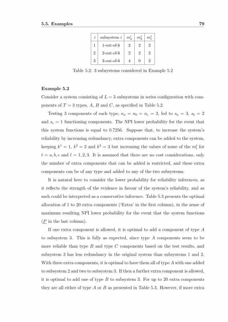
5.5. Examples 79
i subsystem i mia mi
b mic
1 1-out-of-6 2 2 2
2 2-out-of-6 2 2 2
3 3-out-of-6 4 0 2
Table 5.2: 3 subsystems considered in Example 5.2
Example 5.2
Consider a system consisting of L = 3 subsystems in series configuration with com-
ponents of T = 3 types, A, B and C, as specified in Table 5.2.
Testing 3 components of each type, na = nb = nc = 3, led to sa = 3, sb = 2
and sc = 1 functioning components. The NPI lower probability for the event that
this system functions is equal to 0.7256. Suppose that, to increase the system’s
reliability by increasing redundancy, extra components can be added to the system,
keeping k1 = 1, k2 = 2 and k3 = 3 but increasing the values of some of the mtl for
t = a, b, c and l = 1, 2, 3. It is assumed that there are no cost considerations, only
the number of extra components that can be added is restricted, and these extra
components can be of any type and added to any of the two subsystems.
It is natural here to consider the lower probability for reliability inferences, as
it reflects the strength of the evidence in favour of the system’s reliability, and as
such could be interpreted as a conservative inference. Table 5.3 presents the optimal
allocation of 1 to 20 extra components (‘Extra’ in the first column), in the sense of
maximum resulting NPI lower probability for the event that the system functions
(P in the last column).
If one extra component is allowed, it is optimal to add a component of type A
to subsystem 3. This is fully as expected, since type A components seem to be
more reliable than type B and type C components based on the test results, and
subsystem 3 has less redundancy in the original system than subsystems 1 and 2.
With three extra components, it is optimal to have them all of type A with one added
to subsystem 2 and two to subsystem 3. If then a further extra component is allowed,
it is optimal to add one of type B to subsystem 3. For up to 20 extra components
they are all either of type A or B as presented in Table 5.3. However, if more extra

5.5. Examples 80
Extra (m1a,m
1b ,m
1c , m
2a,m
2b ,m
2c ,m
3a,m
3b ,m
3c) P
0 (2,2,2,2,2,2,4,0,2) 0.7256
1 (2,2,2,2,2,2,5,0,2) 0.7896
2 (2,2,2,3,2,2,5,0,2) 0.8302
3 (2,2,2,3,2,2,6,0,2) 0.8675
4 (2,2,2,3,2,2,6,1,2) 0.8907
5 (2,2,2,4,2,2,6,1,2) 0.9087
6 (2,2,2,4,2,2,6,2,2) 0.9244
7 (2,2,2,4,2,2,7,2,2) 0.9345
8 (2,2,2,5,2,2,7,2,2) 0.9437
9 (3,2,2,5,2,2,7,2,2) 0.9513
10 (3,2,2,5,2,2,7,3,2) 0.9584
11 (3,2,2,6,2,2,7,3,2) 0.9635
12 (3,2,2,6,2,2,8,3,2) 0.9684
13 (4,2,2,6,2,2,8,3,2) 0.9716
14 (4,2,2,6,2,2,8,4,2) 0.9748
15 (4,2,2,6,3,2,8,4,2) 0.9782
16 (4,2,2,6,3,2,9,4,2) 0.9806
17 (4,2,2,7,3,2,9,4,2) 0.9828
18 (5,2,2,7,3,2,9,4,2) 0.9845
19 (5,2,2,7,3,2,10,4,2) 0.9862
20 (5,2,2,8,3,2,10,4,2) 0.9876
Table 5.3: Illustration of redundancy and diversity. The red entries indicate the
subsystem and the type of extra component chosen at the specific stage.
5.6. Concluding remarks 81
components are allowed, we expect that type C would also be added, as diversity
in redundancy allocation can result directly from maximisation of reliability, and
is due to the limited knowledge about the reliability of the components of different
types. As Coolen et al. [19] emphasize, this is an important reason for diversity
that is different to the usually mentioned possibility of common-cause failures which
would lead to all components of one type to fail.
In this example, the optimal allocations of up to 20 extra components are all
such that one extra component would just be added to the optimal system structure
derived when one fewer extra component is allowed. For systems with only one
type of component per subsystem and different component types for different sub-
systems, it has been proven that adding extra components sequentially does lead to
optimal redundancy allocation (see Chapter 2). As mentioned before, the basic idea
of optimally allocating one more component, if one can increase m by one without
changing k, is pretty straightforward, as one just calculates the NPI lower proba-
bilities corresponding to all possibilities to add one component to the system and
then chooses the type and subsystem leading to maximum improvement. However,
if one can allocate more than one component, it is not clear that one can proceed
with such one-step-at-a-time optimisation, which would lead to a simple algorithm.
Based on the numerical computations in this example and some further cases we
looked at, we strongly feel that such an algorithm would be optimal, as was the case
for the more basic scenarios we considered before, but we have not yet achieved a
mathematical proof of optimality for the systems in this chapter. In the example
above, all possible scenarios were calculated and the given results are indeed optimal,
so here one-step-at-a-time optimisation does lead to the overall optimal redundancy
allocation in line with our conjecture that this will always lead to optimality for
such systems.
5.6 Concluding remarks
This chapter has presented an important result in the development of NPI for sys-
tem reliability, namely the lower and upper probabilities for the event that a system
5.6. Concluding remarks 82
with multiple subsystems, each a voting system, in series configuration functions
successfully, where the different subsystems can have components of the same types.
However, the mathematical complexity of these results is already quite substantial,
while these systems still have relatively basic structures. In Example 5.2 an open
problem for research was mentioned, namely to investigate whether or not sequen-
tial optimal allocation of extra components leads to optimal redundancy allocation.
To solve a multi-dimensional optimisation problem, it is not generally sufficient to
restrict to sequential one-dimensional optimisations. Of course, the main aim is to
develop NPI for reliability of more complex system structures. Possibly the theory
of signatures [51] may be of use, but the theory of signatures only applies to sys-
tems with a single type of component and it is not clear if it can be generalized to
multiple component types. Further challenges are related to implementation of the
results presented in this chapter for larger systems. In particular for large values
of T and L, computational difficulties may appear due to the very large number
of calculations involved, and it may be possible to derive suitable approximations.
For risk assessment of safety-critical systems, which would only be used if tests had
revealed zero failures [15], a reasonable lower bound for the NPI lower probability
of system functioning may be sufficient to support decisions, with possible use of a
corresponding upper bound for the NPI lower probability to indicate the accuracy
of the approximation.
While these results may be perceived as having a rather abstract nature, they
are readily available for implementation and the implications for practical reliabil-
ity assessment can be considerable. By taking the uncertainty about reliability of
components, resulting from limited test information, explicitly into account, which
results in dependence of the random quantities representing the reliabilities of the
components in the system, the overall system reliability can be very different from
values that are perhaps more in line with intuition, as explained in examples and
discussions in Coolen-Schrijner et al. [29]. This also affects the important aspects
of redundancy and diversity related to system reliability, as briefly discussed in
Example 5.2 and in more detail, but only for a single voting system, in Chapter 4.

Chapter 6
Conclusions
In this thesis, several extensions to Nonparametric Predictive Inference (NPI) for
system reliability were presented. The NPI approach to system reliability is in early
stages of development. It provides a new method for statistical inference on system
reliability on the basis of limited information resulting from component testing.
In Chapter 2, the basic application of NPI for Bernoulli random quantities to
inference on reliability of systems which are series of independent subsystems, with
each subsystem a ki-out-of-mi system with exchangeable components, was presented.
With reliability measured by the NPI lower probability for system functioning, op-
timal redundancy allocation of extra components can be achieved, for any number
of extra components, by sequential one-step optimal allocation. According to this
technique, at each step an extra component is allocated to the subsystem for which
the relative increase in reliability is maximal. The algorithm to determine the op-
timal sequence of adding the extra components to subsystems was described, and
the proof of optimality was given. This result determined how to optimally allocate
additional components for redundancy for any criterion in the case where the cost of
components is irrelevant, or where they are the same for all components. If the costs
of additional components differ per subsystem, and one aims to maximize system
reliability under budget constraints, then the redundancy allocation problem be-
comes more complex. Fortunately this problem is close in nature to the well-known
knapsack problems in discrete optimisation, and can be considered, after a simple
modification, as a 0-1 knapsack problem.
83
Chapter 6. Conclusions 84
In Chapter 3, an important step in the development of NPI for more complex
system structures was introduced. The NPI lower and upper probabilities for func-
tioning of a system consisting of multiple ki-out-of-mi subsystems in a series configu-
ration, with all subsystems consisting of the same type of component, was presented.
This is non-trivial, as the random quantities representing whether the components
in the system function or not, are not independent in the NPI approach, given the
test results. It is important that this dependence is explicitly taken into account,
in particular when there is relatively little information from tests. As a first step
for this research, we generalized NPI for Bernoulli quantities to distinguish between
subgroups of the m future observations, and using a path counting technique we
derived lower and upper probabilities which quantify the reliability of such systems.
In Chapter 4, NPI for reliability of voting systems with multiple component
types was presented. This is a further step in the development of NPI for system
reliability, where more general system structures can be considered. Whilst restrict-
ing attention to a single voting system, this was now allowed to consist of multiple
types of components. They are assumed to perform the same function within the
system, but the test information differs per type of component, and in terms of
their reliability components of the same type are exchangeable and assumed to be
independent of components of other types. In addition to presenting the NPI lower
and upper probabilities for system functioning, we addressed aspects of redundancy
and diversity for such systems, where the benefit of having multiple types of com-
ponents, with only limited test information per component type, was considered in
detail.
In Chapter 5, we introduced a generalization of structure of the systems intro-
duced in the previous three chapters by considering systems with a series structure
where each subsystem is a single voting system consisting of different types of com-
ponents. The important contribution of this chapter is that different subsystems can
contain components of the same types. The results presented in this chapter gener-
alize the results in Chapters 2, 3 and 4, and hence are the main results presented in
this thesis.

Chapter 6. Conclusions 85
Throughout this thesis, numerical examples illustrated some of the general prop-
erties for all systems considered. For example, the NPI upper probability for suc-
cessful system functioning given s successes in n tests is equal to the NPI lower
probability for successful system functioning given s + 1 successes in n tests. The
NPI lower (upper) probability for the case s = 0 (s = n) is equal to 0 (1), which re-
flects that in this case there is no strong evidence that the components can actually
function (fail). The imprecision, that is the difference between corresponding NPI
upper and lower probabilities, tends to decrease as a function of n and increase as
a function of m, although the imprecision tends to become smaller for non-trivial
events if both the upper and lower probabilities get close to either zero or to one. It
will be of interest to study this in more detail, in particular as imprecision seems to
relate logically to the amount of information available and to the number of future
random quantities involved in the event of interest.
The basic idea of optimally allocating one more component, if one can increase
m by one without changing k, is pretty straightforward, as one just calculates the
NPI lower probabilities corresponding to all possibilities to add one component to
the system and then chooses the type and subsystem leading to maximum improve-
ment. However, if one can allocate more than one component, it is not clear that
one can proceed with such one-step-at-a-time optimisation, which would lead to a
simple algorithm. For systems with only one type of component per subsystem and
different component types for different subsystems, it has been proven in Chapter
2 that adding extra components sequentially does lead to optimal redundancy allo-
cation. Numerical examples presented throughout this thesis, and further cases we
looked at, indicate that a similarly attractive algorithm will again be optimal for
the systems considered in Chapters 3, 4 and 5, but proving this turned out to be
rather complicated, and we have not achieved this.
The systems considered in Chapters 4 and 5 consist of multiple types of compo-
nents. One of the main conclusions of these chapters is that considering diversity
of components in a system is important to achieve maximum system reliability in
situations with limited information about component reliability, but the optimal
configuration depends on the actual system structure, with diversity generally most

Chapter 6. Conclusions 86
useful for parallel systems, while for series systems one would not opt for diversity
and only use components of the type that gave the best test results. We only showed
this for the simple systems considered in these chapters, but we strongly feel that
similar conclusions will hold for more general system structures when NPI lower
probabilities are used to express system reliability.
In the reliability literature, system reliability is usually expressed as function
of failure probabilities for components, which are typically assumed to be known.
Under limited information, this will clearly not be the case, and the proper inclu-
sion of uncertainty about components’ failure probabilities is rarely addressed. One
cannot replace parameters representing such failure probabilities by estimates, as
the system reliability is typically a non-linear function of the failure probabilities.
More importantly, any such a classical approach with parameters representing com-
ponents’ failure probabilities does not take into account the interdependence of the
components to be used in the system of interest.
One can use a Bayesian approach, expressing the system reliability via a posterior
predictive distribution, which will take care of this interdependence, but this requires
the use of prior distributions for the parameters, which adds further assumptions
that may be hard to justify. This is particularly clear when considering system
reliability after zero-failure tests, where Bayesian methods will typically lead to a
probability of system functioning that is less than one, while clearly the test data do
not strongly suggest that components might actually fail. The use of lower and upper
probabilities in reliability is attractive in such situations as the upper probability of
system functioning, given no test failures, can be equal to one (as the NPI upper
probabilities are), reflecting no evidence that things can go wrong. In such cases,
the corresponding lower probability may be of most use, as it reflects the amount
of evidence available in favour of system functioning, and as it enables cautious
inference which is often deemed appropriate in risk analysis. The fact that the NPI
lower and upper probabilities result from combinatorial arguments, based only on
an exchangeability assumption and an underlying latent variable representation, is
also attractive.

Chapter 6. Conclusions 87
NPI lower and upper probabilities for system reliability are based on combina-
torics, so the computation time will increase for more substantial systems. However,
there are no complex integrals involved (as e.g. is typically the case in Bayesian
statistics), and as all sums are finite there are no major computational difficul-
ties. For large systems it may be required to consider approximations for the sums
involved in deriving the NPI lower and upper probabilities, but NPI is not yet de-
veloped to the stage where this has become relevant. If more test data become
available, updating the NPI lower and upper probabilities occurs by calculating
them again using all combined information, there is no straightforward sequential
updating algorithm available as is the case in Bayesian statistics.
The theory of system signatures [51] provides a powerful framework for reliability
assessment for systems consisting of exchangeable components. Coolen and Al-
nefaiee [20] showed how signatures can be used within NPI to derive lower and upper
survival functions for the failure time of such systems, given failure times of tested
components, and to compare the reliability of two such systems. Signatures can
also be used for reliability quantification for systems for which only failure or non-
failure upon request for functioning is of interest, so without explicit focus on failure
time. Applying this to systems with exchangeable components will be relatively
straightforward and will generalize the results in Chapter 3, and analysis based
on signatures might facilitate the proof of optimality of the presented redundancy
allocation algorithm. This is left as a topic for future research.
Although a nonparametric approach as presented in this thesis is attractive, it
has obvious limitations. For example, if NPI were developed further in order to
take ageing of technical components into account, the huge amount of data needed
to describe the effects of ageing without the use of a parametric model will make
the approach of little practical value. One of the main research challenges for NPI
will be to combine it with partial parametric modelling to model aspects of ageing
using specific processes. This may lead to a novel semi-parametric approach that
could be of benefit to a wide range of applications. The use of lower and upper
probabilities in combination with stochastic processes is an exciting topic area for
future research, which has not attracted much attention so far.

Chapter 6. Conclusions 88
Throughout this thesis, several research challenges related to this NPI approach
to system reliability and redundancy allocation have been mentioned. Several of
these require some further development of NPI theory and methods, whereas others
provide further analytical challenges or require development of suitable computa-
tional algorithms.
Appendix A
Brief guide to notation
A(n) Hill’s inferential assumption.
ci cost to add one extra component to subsystem i.
C(j) total cost of these additional components being added to the whole system.
ji number of additional components added to subsystem i.
k minimum number of functioning components for a k-out-of-m system to function.
ki minimum number of functioning components for the subsystem i to function.
L total number of subsystems in the considered system.
m total number of components in the considered system.
mi total number of components in subsystem i.
mt total number of components of type t in the considered system.
mit total number of components of type t in subsystem i.
n total number of components that have been tested.
nt number of components of type t that have been tested.
P (A) NPI lower probability for event A.
P (A) NPI upper probability for event A.
ρ(i, ji) factor with which the NPI lower probability for successful functioning of subsys-
tem i increases when ji + 1 instead of ji extra components are added.
s number of successfully tested components.
st number of successfully tested components of type t.
T total number of component types in the considered system.
Y ba random number of successes in trials a to b.
89

Bibliography
[1] Aboalkhair, A. M., MacPhee, I.M. & Coolen, F.P.A. (2009). Nonparametric
predictive system reliability with redundancy allocation following component
testing. Proceedings Advances in Risk and Reliability Technology Symposium,
2009, L. Bartlett (Eds), 396-407.
[2] Aboalkhair, A.M., Coolen, F.P.A. & MacPhee, I.M. (2010). Nonparamet-
ric predictive inference for reliability of voting systems with multiple com-
ponent types. Proceedings 3rd International Conference on Accelerated Life
Testing, Reliability-based Analysis and Design. Clermont-Ferrand (France)
Chateauneuf, Nikulin & Guerin (Eds), 175-182.
[3] Aboalkhair, A.M., Coolen, F.P.A. & MacPhee, I.M. (2011). Nonparametric
predictive inference for system reliability with subsystems consisting of multi-
ple component types. Proceedings Advances in Risk and Reliability Technology
Symposium, 2011, D. Prescott and R. Remenyte-Prescott (Eds), 322-339.
[4] Aboalkhair, A.M., Coolen, F.P.A. & MacPhee, I.M. (2012). Nonparamet-
ric predictive inference for reliability of a series of subsystems with multi-
ple component types. Advances in Safety, Reliability and Risk Management,
Berenguer, Grall & Guedes Soares (Eds) Taylor & Francis Group, London,
ISBN 978-0-415-68379-1, 1069-1077.
[5] Aboalkhair, A.M., Coolen, F.P.A. & MacPhee, I.M. (2012). Nonparametric
predictive inference for reliability of a k-out-of-m : G system with multiple
component types. In submission
90
Bibliography 91
[6] Aboalkhair, A.M., Coolen, F.P.A. & MacPhee, I.M. (2012). Nonparametric
predictive reliability of series of voting systems. In submission
[7] Andrews, J.D. and Moss, T.R. (2002). Reliability and Risk Assessment (2nd
Ed.). London: Professional Engineering Publishing Ltd.
[8] Augustin, T. and Coolen, F.P.A. (2004). Nonparametric predictive inference
and interval probability. Journal of Statistical Planning and Inference 124,
251-272.
[9] Birnbaum, Z. W., Esary, J. D. and Saunders, S. (1961). Multi-component
systems and structures and their reliability. Technometrics 3, 5577.
[10] Boole, G. (1854). An Investigation of the Laws of Thought on which are
founded the Mathematical Theories of Logic and Probabilities. Walton and
Maberley, London.
[11] Cai, K-Y. (1996). Introduction to Fuzzy Reliability. Boston: Kluwer Academic
Publishers.
[12] Coolen, F.P.A. (1998). Low structure imprecise predictive inference for Bayes’
problem. Statistics & Probability Letters 36, 349-357.
[13] Coolen, F.P.A. (2004). On the use of imprecise probabilities in reliability.
Quality and Reliability Engineering International 20, 193-202.
[14] Coolen, F.P.A. (2006). On nonparametric predictive inference and objective
Bayesianism. Journal of Logic, Language and Information 15, 21-47.
[15] Coolen, F.P.A. (2006). On probabilistic safety assessment in case of zero fail-
ures. Journal of Risk and Reliability 220, 105-114.
[16] Coolen, F.P.A. (2007). Nonparametric prediction of unobserved failure modes.
Journal of Risk and Reliability 221, 207-216.
[17] Coolen, F.P.A. (2010) International Encyclopaedia of Statistical Sciences
(Nonparametric Predictive Inference chapter). Springer, Berlin.
Bibliography 92
[18] Coolen, F.P.A., Aboalkhair, A.M. & MacPhee, I.M. (2009). Nonparametric
predictive system reliability with all subsystems consisting of one type of com-
ponent. In M.J. Kallen & S.P. Kuniewski (Eds), Risk and Decision Analysis in
Maintenance Optimization and Flood Management, Amsterdam: IOS Press,
85-98.
[19] Coolen, F.P.A., Aboalkhair, A.M. & MacPhee, I.M. (2011). Diversity in sys-
tem reliability following component testing, Journal of the Safety and Relia-
bility Society 30, 75-93.
[20] Coolen, F.P.A. and Al-nefaiee, A.H. (2012). Nonparametric predictive infer-
ence for failure times of systems with exchangeable components, Journal of
Risk and Reliability to appear.
[21] Coolen, F.P.A. and Augustin, T. (2005). Learning from multinomial data:
a nonparametric predictive alternative to the Imprecise Dirichlet Model. In:
T. Seidenfeld, R. Nau and F.G. Cozman (Eds.), ISIPTA’05 - Proceedings
of the Fourth International Symposium on Imprecise Probabilities and Their
Applications, Carnegie Mellon University, pp. 125-134.
[22] Coolen, F.P.A. and Augustin, T. (2009). A nonparametric predictive alter-
native to the Imprecise Dirichlet Model: the case of a known number of cate-
gories. International Journal of Approximate Reasoning 50, 217-230.
[23] Coolen, F.P.A. and Coolen-Schrijner, P. (2005). Nonparametric predictive re-
liability demonstration for failure-free periods. IMA Journal of Management
Mathematics 16, 1-11.
[24] Coolen, F.P.A. and Coolen-Schrijner, P. (2007). Nonparametric predictive
comparison of proportions. Journal of Statistical Planning and Inference 137,
23-33.
[25] Coolen, F.P.A. and Yan, K.J. (2004) Nonparametric predictive inference with
right-censored data. Journal of Statistical Planning and Inference 126, 25-54.
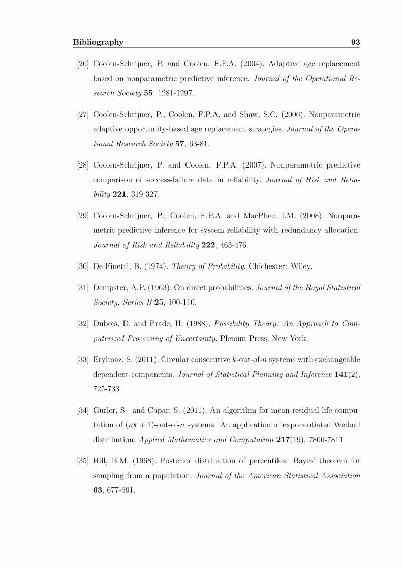
Bibliography 93
[26] Coolen-Schrijner, P. and Coolen, F.P.A. (2004). Adaptive age replacement
based on nonparametric predictive inference. Journal of the Operational Re-
search Society 55, 1281-1297.
[27] Coolen-Schrijner, P., Coolen, F.P.A. and Shaw, S.C. (2006). Nonparametric
adaptive opportunity-based age replacement strategies. Journal of the Opera-
tional Research Society 57, 63-81.
[28] Coolen-Schrijner, P. and Coolen, F.P.A. (2007). Nonparametric predictive
comparison of success-failure data in reliability. Journal of Risk and Relia-
bility 221, 319-327.
[29] Coolen-Schrijner, P., Coolen, F.P.A. and MacPhee, I.M. (2008). Nonpara-
metric predictive inference for system reliability with redundancy allocation.
Journal of Risk and Reliability 222, 463-476.
[30] De Finetti, B. (1974). Theory of Probability. Chichester: Wiley.
[31] Dempster, A.P. (1963). On direct probabilities. Journal of the Royal Statistical
Society, Series B 25, 100-110.
[32] Dubois, D. and Prade, H. (1988), Possibility Theory: An Approach to Com-
puterized Processing of Uncertainty. Plenum Press, New York.
[33] Erylmaz, S. (2011). Circular consecutive k-out-of-n systems with exchangeable
dependent components. Journal of Statistical Planning and Inference 141(2),
725-733
[34] Gurler, S. and Capar, S. (2011). An algorithm for mean residual life compu-
tation of (nk + 1)-out-of-n systems: An application of exponentiated Weibull
distribution. Applied Mathematics and Computation 217(19), 7806-7811
[35] Hill, B.M. (1968). Posterior distribution of percentiles: Bayes’ theorem for
sampling from a population. Journal of the American Statistical Association
63, 677-691.
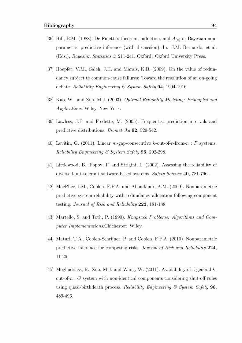
Bibliography 94
[36] Hill, B.M. (1988). De Finetti’s theorem, induction, and A(n) or Bayesian non-
parametric predictive inference (with discussion). In: J.M. Bernardo, et al.
(Eds.), Bayesian Statistics 3, 211-241. Oxford: Oxford University Press.
[37] Hoepfer, V.M., Saleh, J.H. and Marais, K.B. (2009). On the value of redun-
dancy subject to common-cause failures: Toward the resolution of an on-going
debate. Reliability Engineering & System Safety 94, 1904-1916.
[38] Kuo, W. and Zuo, M.J. (2003). Optimal Reliability Modeling: Principles and
Applications. Wiley, New York.
[39] Lawless, J.F. and Fredette, M. (2005). Frequentist prediction intervals and
predictive distributions. Biometrika 92, 529-542.
[40] Levitin, G. (2011). Linear m-gap-consecutive k-out-of-r-from-n : F systems.
Reliability Engineering & System Safety 96, 292-298.
[41] Littlewood, B., Popov, P. and Strigini, L. (2002). Assessing the reliability of
diverse fault-tolerant software-based systems. Safety Science 40, 781-796.
[42] MacPhee, I.M., Coolen, F.P.A. and Aboalkhair, A.M. (2009). Nonparametric
predictive system reliability with redundancy allocation following component
testing. Journal of Risk and Reliability 223, 181-188.
[43] Martello, S. and Toth, P. (1990). Knapsack Problems: Algorithms and Com-
puter Implementations.Chichester: Wiley.
[44] Maturi, T.A., Coolen-Schrijner, P. and Coolen, F.P.A. (2010). Nonparametric
predictive inference for competing risks. Journal of Risk and Reliability 224,
11-26.
[45] Moghaddass, R., Zuo, M.J. and Wang, W. (2011). Availability of a general k-
out-of-n : G system with non-identical components considering shut-off rules
using quasi-birthdeath process. Reliability Engineering & System Safety 96,
489-496.
Bibliography 95
[46] Pate-Cornell, M.E., Dillon, R.L. and Guikema, S.D. (2004). On the limitations
of redundancies in the improvement of system reliability. Risk Analysis 24,
1423-1436.
[47] Rahrouh, M., Coolen, F.P.A. and Coolen-Schrijner, P. (2006). Bayesian relia-
bility demonstration for systems with redundancy. Journal of Risk and Relia-
bility 220, 137-145.
[48] Ruiz-Castro, J. E. and Quan-Lin Li (2011). Algorithm for a general discrete
k−out-of−n : G system subject to several types of failure with an indefinite
number of repairpersons. European Journal of Operational Research, 211(1),
97-111
[49] Senz-de-Cabezn, E. and Wynn, H. P. (2011). Computational algebraic algo-
rithms for the reliability of generalized k-out-of-n and related systems. Math-
ematics and Computers in Simulation 82(1), 68-78
[50] Salehi, E.T., Asadi,M. and Erylmaz, S. (2011). Reliability analysis of consec-
utive k-out-of-n systems with non-identical components lifetimes. Journal of
Statistical Planning and Inference 141(8) 2920-2932
[51] Samaniego, F (2007). System Signatures and their Applications in Engineering
Reliability. New York: Springer.
[52] Tian, Z., Zuo, M. J. and Yam, R. C. (2009). Multi-state k-out-of-n systems
and their performance evaluation. IIE Transactions 41, 32-44.
[53] Torres-Echeverria, A.C., Martorell, S. and Thompson, H.A. (2011). Modeling
safety instrumented systems with MooN voting architectures addressing sys-
tem reconfiguration for testing. Reliability Engineering & System Safety 96,
545-563.
[54] Utkin, L.V. and Coolen, F.P.A. (2007). Imprecise reliability: an introductory
overview. In: G. Levitin (Ed.), Computational Intelligence in Reliability En-
gineering, Volume 2: New Metaheuristics, Neural and Fuzzy Techniques in
Reliability, 261-306. New York: Springer.

Bibliography 96
[55] Vaurio, J.K. (1995). The probabilistic modeling of external common cause
failure shocks in redundant systems. Reliability Engineering & System Safety
50, 97-107.
[56] Vaurio, J.K. (2011). Unavailability equations for k-out-of-n systems. Reliability
Engineering & System Safety 96, 350-352.
[57] Walley, P. (1991). Statistical Reasoning with Imprecise Probabilities. London:
Chapman and Hall.
[58] Weichselberger, K. (2000). The theory of interval-probability as a unifying
concept for uncertainty. International Journal of Approximate Reasoning 24,
149-170.
[59] Weichselberger, K. (2001). Elementare Grundbegriffe einer allgemeineren
Wahrscheinlichkeitsrechnung I. Intervallwahrscheinlichkeit als umfassendes
Konzept. Heidelberg: Physika.
[60] Williamson, J. (2004). Philosophies of probability: objective Bayesianism
and its challenges. Handbook of the Philosophy of Mathematics, Volume 9 of
theHandbook of the Philosophy of Science, Irvine, ed., Elsevier.