Nonparametric Identi�cation of a Binary RandomFactor in Cross Section Data

Yingying Dong and Arthur Lewbel�

California State University Fullerton and Boston College

Original January 2009, revised March 2011

Abstract

Suppose V and U are two independent mean zero random variables, where Vhas an asymmetric distribution with two mass points and U has some zero oddmoments (having a symmetric distribution su¢ ces). We show that the distrib-utions of V and U are nonparametrically identi�ed just from observing the sumV +U , and provide a pointwise rate root n estimator. This can permit point iden-ti�cation of average treatment e¤ects when the econometrician does not observewho was treated. We extend our results to include covariates X, showing that wecan nonparametrically identify and estimate cross section regression models of theform Y = g(X;D�) + U , where D� is an unobserved binary regressor.

JEL Codes: C25, C21Keywords: Mixture model, Random e¤ects, Binary, Unobserved factor, Unob-served regressor, Nonparametric identi�cation, Deconvolution, Treatment

1 Introduction

We propose a method of nonparametrically identifying and estimating cross section

regression models that contain an unobserved binary regressor or treatment, or equiva-

lently an unobserved random e¤ect that can take on two values. For example, suppose

an experiment (natural or otherwise) with random or exogenous assignment to treat-

ment was performed on some population, but we only have survey data collected in the�Corresponding Author: Arthur Lewbel, Department of Economics, Boston Col-

lege, 140 Commonwealth Avenue, Chestnut Hill, MA, 02467, USA. (617)-552-3678, lew-bel@bc.edu,http://www2.bc.edu/~lewbel/

1

region where the experiment occured, and this survey does not report which (or even

how many) individuals were treated. Then, given our assumptions, we can point identify

the average treatment e¤ect in this population and the probability of treatment, despite

not observing who was treated.

No instruments or proxies for the unobserved binary regressor or treatment need to

be observed. Identi�cation is obtained by assuming that the unobserved exogenously

assigned treatment or binary regressor e¤ect is a location shift of the observed outcome,

and that the regression or conditional outcome errors have zero low order odd moments

(a su¢ cient condition for which is symmetrically distributed errors). These identifying

assumptions provide moment conditions that can be used to construct either an ordinary

generalized method of moments (GMM) estimator, or in the presence of covariates, a

nonparametric local GMM estimator for the model.

The zero low order odd moments used for identi�cation here can arise in a number

of contexts. Normal errors are of course symmetric and so have all odd moments equal

to zero, and normality arises in many models such as those involving central limit theo-

rems, e.g., Gibrat�s law for wage or income distributions. Di¤erences of independently,

identically distributed errors, or more generally of exchangable errors such as those fol-

lowing ARMA processes, are also symmetrically distributed (see, e.g., proposition 1 of

Honore 1992). So, e.g., two period panel models with �xed e¤ects and ARMA errors

will generally have errors that are symmetric after time di¤erencing. Our results could

therefore be applied in a two period panel where individuals can have an unobserved

mean shift at any time (corresponding to the unobserved binary regressor), �xed e¤ects

(which are di¤erenced away) and exchangable remaining errors (which yield symmetric

errors after di¤erencing). Below we give other more speci�c examples of models with

the required odd moments being zero.

Ignoring covariates for the moment, suppose Y = h + V + U , where V and U are

2

independent mean zero random variables and h is a constant. The random V equals

either b0 or b1 with unknown probabilities p and 1 � p respectively, where p does not

equal a half, i.e., V is asymmetrically distributed. U is assumed to have its �rst few odd

moments equal to zero. We observe a sample of observations of the random variable Y ,

and so can identify the marginal distribution of Y , but we do not observe h, V , or U .

We �rst show that the constant h and the distributions of V and U are nonparamet-

rically identi�ed just from observing Y . The only regularity assumption required is that

some higher moments of Y exist. More precisely, the �rst three odd moments of U must

be zero (and so also exist for Y ) for local identi�cation, while having the �rst �ve odd

moments of U equal zero su¢ ces for global identi�cation.

We also provide estimators for the distributions of V and U . We show that the

constant h, the probability mass function of V , moments of the distribution of U , and

points of the distribution function of U can all be estimated using GMM. Unlike common

deconvolution estimators that can converge at slow rates, we estimate the distributions

of V and U , and the density of U (if it is continuous) at the same rates of convergence

as if V and U were separately observed, instead of just observing their sum.

We do not assume that the supports of V or U are known, so estimation of the

distribution of V means identifying and estimating both of its support points b0 and b1,

as well as the probabilities p and 1� p, respectively, of V equaling b0 or b1.

One can write V as V = b1D�+b0 (1�D�) where D� is an unobserved binary indica-

tor. For example, if D� is the unobserved indicator of exogenously assigned treatment,

then b1 � b0 is the average treatment e¤ect, p is the probability of treatment, and U

describes the remaining heterogeneity of outcomes Y (here treatment is assumed to only

cause a shift in outcome means)

We also show how these results can be extended to allow for covariates. If h depends

on a vector of covariates X while V and U are independent of X, then we obtain the

3

random e¤ects regression model Y = h (X) + V + U , which is popular for panel data,

but which we identify and estimate just from cross section data.

More generally, we allow both h and the distributions of V and U to depend in

unknown ways on X. This is equivalent to nonparametric identi�cation and estima-

tion of a regression model containing an unobserved binary regressor. The regression

model is Y = g(X;D�) + U , where g is an unknown function, D� is an unobserved

binary regressor (or unobserved indicator of treatment) that equals zero with unknown

probability p (X) and one with probability 1 � p(X), while U is a random error with

an unknown conditional distribution FU (U j X) having its �rst few odd moments equal

to zero (conditional symmetry conditioning on X su¢ ces). The unobserved random

variables U and D� are assumed to be conditionally independent, conditioning upon X.

By de�ning h (x) = E (Y j X = x) = E [g(X;D�) j X = x], V = g(X;D�) � h(X) and

U = Y � h (X)� V , this regression model can then be rewritten as Y = h (X) +V +U ,

where h (x) is a nonparametric regression function of Y onX, and the two support points

of V conditional on X = x are then bd (x) = g(x; d)�h(x) for d = 0; 1. Kitamura (2004)

provides some nonparametric identi�cation results for this model by placing constraints

on how the distributions can depend upon X, while we place no such restrictions on the

distribution of X and instead restrict the shape of the distribution of V .

The assumptions we impose on U in Y = g(X;D�) + U are common assumptions in

regression models, e.g., they allow the error U to be heteroskedastic with respect to X,

and they hold, e.g., if U given X is normal (though normality is not required). Also,

regression model errors U are sometimes interpreted as measurement error in Y , and

measurement errors are often assumed to be symmetric.

If D� is an unobserved treatment indicator, then g(X; 1)� g(X; 0) is the conditional

average treatment e¤ect, which may be averaged over X to obtain an unconditional

average treatment e¤ect. Symmetry of errors is not usually assumed for treatment

4

models, but suppose we have panel data (two periods of observations) and all treatments

occur in one of the two periods. Then as noted above the required symmetry of U

errors would result automatically from time di¤erencing the data, given the standard

panel model assumption of individual speci�c �xed e¤ects plus independently, identically

distributed (or more generally ARMA or other exchangable) errors.

Another possible application of these extensions is a stochastic frontier model, where

Y is the log of a �rm�s output, X are factors of production, and D� indicates whether

the �rm operates e¢ ciently at the frontier, or ine¢ ciently. Existing stochastic frontier

models obtain identi�cation either by assuming parametric functional forms for both the

distributions of V and U , or by using panel data and assuming that each �rm�s individual

e¢ ciency level is a �xed e¤ect that is constant over time. See, e.g., Kumbhakar et. al.

(2007) and Simar and Wilson (2007). In contrast, our assumptions and associated

estimators could be used to estimate a nonparametric stochastic frontier model using

cross section data, given the restriction that unobserved e¢ ciency is indexed by a binary

D�. Note that virtually all stochastic frontier models based on cross section data assume

U given X is symmetrically distributed.

Dong (2008) empirically estimates a model where Y = h (X) + V + U , based on

symmetry of U and using moments similar to the exponentials we suggest in an extension

section. Our results formally prove identi�cation of Dong�s model, and our estimator is

more general in that it allows V and the distribution of U to depend in arbitrary ways

on X. Hu and Lewbel (2007) also nonparametrically identify some features of a model

containing an unobserved binary regressor, using either a type of instrumental variable

or an assumption of conditional independence of low order moments.

Models that allocate individuals into various types, as D� does, are common in

the statistics and marketing literatures. Examples include cluster analysis, latent class

analysis, and mixture models (see, e.g., Clogg 1995 and Hagenaars and McCutcheon

5

2002). Our model resembles a �nite (two distribution) mixture model, but di¤ers cru-

cially in that, for identi�cation, �nite mixture models usually require the distributions

being mixed to be parametrically speci�ed, while in our model U is nonparametric.

While general mixture models are more �exible than ours in allowing for more than two

groups and permitting the U distribution to vary across groups, ours is more �exible

in letting U be nonparametric, essentially allowing for an in�nite number of parameters

versus �nitely parameterized mixtures.

Some mixture models can be nonparametrically identi�ed by observing draws of vec-

tors of data, where the number of elements of the observed vectors is larger than the

number of distributions being mixed. Examples include Hall and Zhou (2003) and Kasa-

hara and Shimotsu (2009). In contrast, we obtain identi�cation with a scalar Y . As

noted above, Kitamura (2004) also obtains nonparametric identi�cation with a scalar

Y , but does so by requiring observation of a covariate that a¤ects the component distri-

butions with some restrictions. Another closely related mixture model result is Bordes,

Mottelet, and Vandekerkhove (2006), who impose strictly stronger conditions than we

do, including that U is symmetric and continuously distributed.

Also related is the literature on mismeasured binary regressors, where identi�cation

generally requires instruments. An exception is Chen, Hu and Lewbel (2008). Like

our Theorem 1 below, they exploit error symmetry for identi�cation, but unlike this

paper they assume that the binary regressor is observed, though with some measurement

(classi�cation) error, instead of being completely unobserved. A more closely related

result is Heckman and Robb (1985), who like us use zero low order odd moments to

identify a binary e¤ect, though theirs is a restricted e¤ect that is strictly nested in our

results. Error symmetry has also been used to obtain identi�cation in a variety of other

econometric contexts, e.g., Powell (1986).

There are a few common ways of identifying the distributions of random variables

6

given just their sum. One method of identi�cation assumes that the exact distribution

of one of the two errors is known a priori, (e.g., from a validation sample as is common in

the statistics literature on measurement error; see, e.g., Carroll, et. al. 2006) and using

deconvolution to obtain the distribution of the other one. For example, if U were normal,

one would need to know a priori its mean and variance to estimate the distribution of V .

A second standard way to obtain identi�cation is to parameterize both the distributions

of V and U , as in most of the latent class literature or in the stochastic frontier literature

(see, e.g., Kumbhakar and Lovell 2000) where a typical parameterization is to have V

be log normal and U be normal. Panel data models often have errors of the form V +U

that are identi�ed either by imposing speci�c error structures or assuming one of the

errors is �xed over time (see, e.g., Baltagi 2008 for a survey of random e¤ects and

�xed e¤ects panel data models). Past nonparametric stochastic frontier models have

similarly required panel data for identi�cation, as described above. In contrast to all

these identi�cation methods, in our model both U and V have unknown distributions,

and no panel data are required.

The next section contains our main identi�cation result. We then provide moment

conditions for estimating the model, including the distribution of V (its support points

and the associated probability mass function), using ordinary GMM. Next we give es-

timators for the distribution and density function of U . We provide a Monte Carlo

analysis showing that our estimator performs reasonably well even compared to infeasi-

ble maximum likelihood estimation. This is followed by some extensions showing how

our identi�cation and estimation methods can be augmented to provide additional mo-

ments for estimation, and to allow for covariates. Proofs are in the Appendix.

7

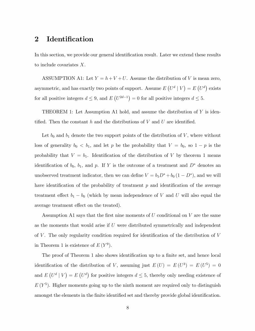
2 Identi�cation

In this section, we provide our general identi�cation result. Later we extend these results

to include covariates X.

ASSUMPTION A1: Let Y = h+V +U . Assume the distribution of V is mean zero,

asymmetric, and has exactly two points of support. Assume E�Ud j V

�= E

�Ud�exists

for all positive integers d � 9, and E�U2d�1

�= 0 for all positive integers d � 5.

THEOREM 1: Let Assumption A1 hold, and assume the distribution of Y is iden-

ti�ed. Then the constant h and the distributions of V and U are identi�ed.

Let b0 and b1 denote the two support points of the distribution of V , where without

loss of generality b0 < b1, and let p be the probability that V = b0, so 1 � p is the

probability that V = b1. Identi�cation of the distribution of V by theorem 1 means

identi�cation of b0, b1, and p. If Y is the outcome of a treatment and D� denotes an

unobserved treatment indicator, then we can de�ne V = b1D�+ b0 (1�D�), and we will

have identi�cation of the probability of treatment p and identi�cation of the average

treatment e¤ect b1 � b0 (which by mean independence of V and U will also equal the

average treatment e¤ect on the treated).

Assumption A1 says that the �rst nine moments of U conditional on V are the same

as the moments that would arise if U were distributed symmetrically and independent

of V . The only regularity condition required for identi�cation of the distribution of V

in Theorem 1 is existence of E (Y 9).

The proof of Theorem 1 also shows identi�cation up to a �nite set, and hence local

identi�cation of the distribution of V , assuming just E (U) = E (U3) = E (U5) = 0

and E�Ud j V

�= E

�Ud�for positive integers d � 5, thereby only needing existence of

E (Y 5). Higher moments going up to the ninth moment are required only to distinguish

amongst the elements in the �nite identi�ed set and thereby provide global identi�cation.

8

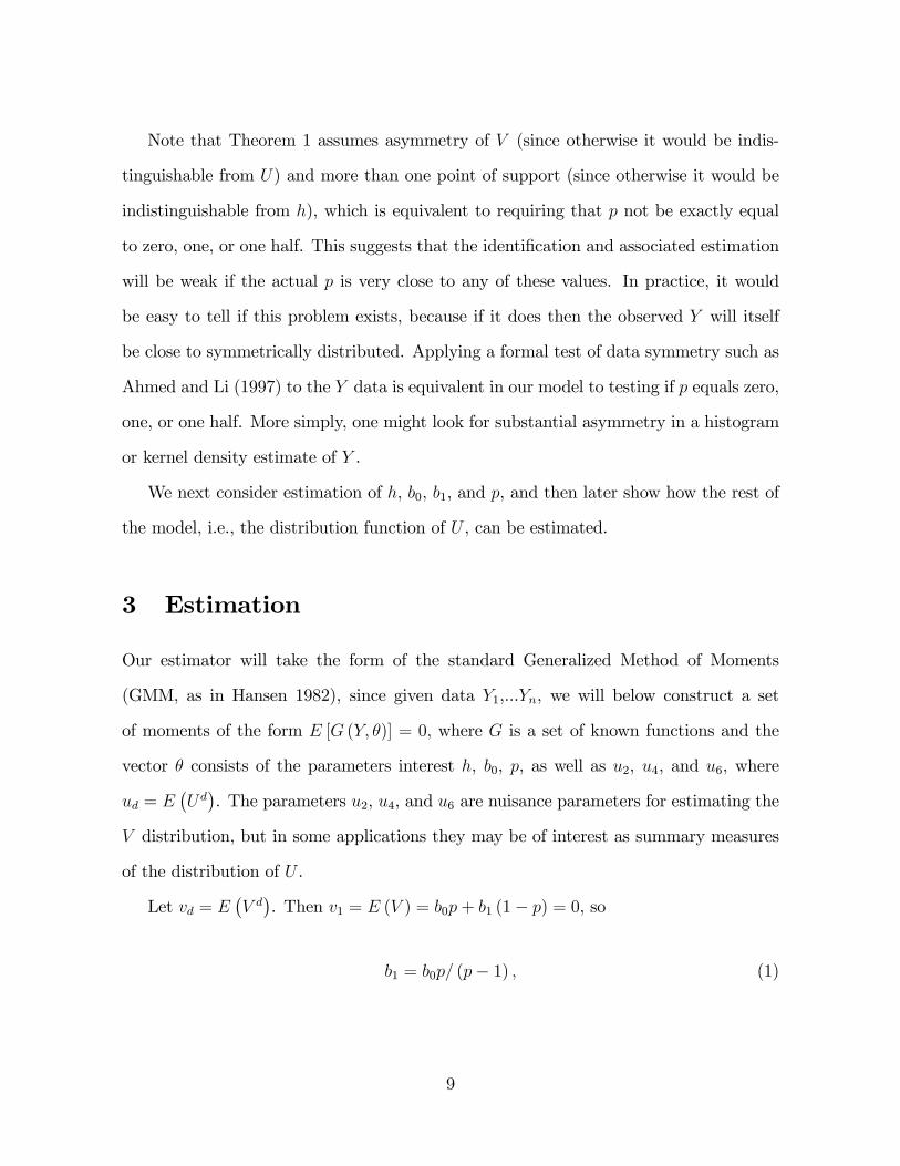
Note that Theorem 1 assumes asymmetry of V (since otherwise it would be indis-

tinguishable from U) and more than one point of support (since otherwise it would be

indistinguishable from h), which is equivalent to requiring that p not be exactly equal

to zero, one, or one half. This suggests that the identi�cation and associated estimation

will be weak if the actual p is very close to any of these values. In practice, it would

be easy to tell if this problem exists, because if it does then the observed Y will itself

be close to symmetrically distributed. Applying a formal test of data symmetry such as

Ahmed and Li (1997) to the Y data is equivalent in our model to testing if p equals zero,

one, or one half. More simply, one might look for substantial asymmetry in a histogram

or kernel density estimate of Y .

We next consider estimation of h, b0, b1, and p, and then later show how the rest of

the model, i.e., the distribution function of U , can be estimated.

3 Estimation

Our estimator will take the form of the standard Generalized Method of Moments

(GMM, as in Hansen 1982), since given data Y1,...Yn, we will below construct a set

of moments of the form E [G (Y; �)] = 0; where G is a set of known functions and the

vector � consists of the parameters interest h, b0, p, as well as u2, u4, and u6, where

ud = E�Ud�. The parameters u2, u4, and u6 are nuisance parameters for estimating the

V distribution, but in some applications they may be of interest as summary measures

of the distribution of U .

Let vd = E�V d�. Then v1 = E (V ) = b0p+ b1 (1� p) = 0, so

b1 = b0p= (p� 1) ; (1)

9

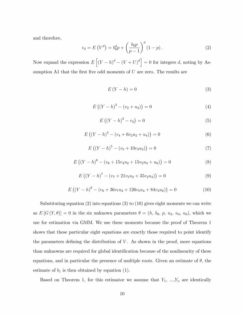
and therefore,

vd = E�V d�= bd0p+

�b0p

p� 1

�d(1� p) : (2)

Now expand the expression Eh(Y � h)d � (V + U)d

i= 0 for integers d, noting by As-

sumption A1 that the �rst �ve odd moments of U are zero. The results are

E (Y � h) = 0 (3)

E�(Y � h)2 � (v2 + u2)

�= 0 (4)

E�(Y � h)3 � v3

�= 0 (5)

E�(Y � h)4 � (v4 + 6v2u2 + u4)

�= 0 (6)

E�(Y � h)5 � (v5 + 10v3u2)

�= 0 (7)

E�(Y � h)6 � (v6 + 15v4u2 + 15v2u4 + u6)

�= 0 (8)

E�(Y � h)7 � (v7 + 21v5u2 + 35v3u4)

�= 0 (9)

E�(Y � h)9 � (v9 + 36v7u2 + 126v5u4 + 84v3u6)

�= 0 (10)

Substituting equation (2) into equations (3) to (10) gives eight moments we can write

as E [G (Y; �)] = 0 in the six unknown parameters � = (h, b0, p, u2, u4, u6), which we

use for estimation via GMM. We use these moments because the proof of Theorem 1

shows that these particular eight equations are exactly those required to point identify

the parameters de�ning the distribution of V . As shown in the proof, more equations

than unknowns are required for global identi�cation because of the nonlinearity of these

equations, and in particular the presence of multiple roots. Given an estimate of �, the

estimate of b1 is then obtained by equation (1).

Based on Theorem 1, for this estimator we assume that Y1, ...,Yn are identically

10

distributed (or more precisely, have identical �rst nine moments), however, the Y ob-

servations do not need to be independent, since GMM estimation theory permits some

serial dependence in the data. Standard GMM limiting distribution theory applied to

our moments provides root n consistent, asymptotically normal estimates of � and hence

of h and of the distribution of V , (i.e., the support points b0 and b1 and the probability

p, where bb1 is obtained by bb1 = bb0bp= (bp� 1) from equation 1). Without loss of generalitywe have imposed b0 < b1 (if this is violated then the de�nitions of these two parameters

can be switched to make the inequality hold), and this along with E (V ) = 0 implies

that bb0 is negative and bb1 is positive, which may be imposed on estimation. One couldalso impose that bp lie between zero and one, and that bu2, bu4, and bu6 be positive.One might anticipate poor empirical results, and great sensitivity to outliers or ex-

treme observations of Y , given the use of such high order moments for estimation. For

example, Altonji and Segal (1996) document bias in GMM estimates associated with

just second order moments. However, we found that these problems rarely arose in our

monte carlo simulations (in applications one would want to carefully scale Y to avoid the

e¤ects of computer rounding errors based on inverting matrix entries of varying orders

of magnitude). We believe the reason the estimator performs reasonably well is that

only lower order moments are required for local identi�cation, up to a small �nite set of

values. The higher order moments (speci�cally those above the �fth) are only needed

for global identi�cation to distinguish between these few possible multiple solutions of

the low order polynomials. For example, if by the low order moments b1 was identi�ed

up to a value in the neighborhood of either 1 or of 3, then even poorly estimated higher

moments could succeed in distinguishing between these two neighborhoods, by having a

sample GMM moment mean be substantially closer to zero in the neighborhood of one

value rather than the other.

In an extension section we describe how additional moments could be constructed for

11

estimation based on symmetry of U . These alternative moments might be employed in

applications where the polynomial based moments are found to be problematic. Another

possibility would be to Winsorize extreme observations of the Y data prior to estimation

to robustify the higher moment estimates.

4 The Distribution of U

For any random variable Z, let FZ denote the marginal cumulative distribution function

of Z. De�ne " = V + U . De�ne FKU (u) by

FKU (u) =K�1Xk=0

�1� p

p

�k1

pF" (u+ b0 + (b0 � b1) k) if p > 1=2 otherwise

FKU (u) =K�1Xk=0

�p

1� p

�k1

1� pF" (u+ b1 + (b1 � b0) k) if p < 1=2

The proof of Theorem 1 shows that FU (u) = FKU (u)+RK , where 0 � RK � min��

p1�p

�K;�1�pp

�K�,

so the remainder term RK ! 0 as K ! 1 (since p = 1=2 is ruled out). This suggests

that FU could be estimated by FKU (u) after replacing F" with the empirical distribution

of Y � bh, replacing b0, b1, and p with their estimates, and letting K !1 as N !1.

However, under the assumption that U is symmetrically distributed, the following

theorem provides a more convenient way to estimate the distribution function of U .

De�ne

(u) =[F" (�u+ b0)� 1] p+ F" (u+ b1) (1� p)

1� 2p : (11)

THEOREM 2: Let Assumption A1 hold. Assume U is symmetrically distributed.

Then

FU (u) = (u)�(�u) + 1

2: (12)

Theorem 2 provides a direct expression for the distribution of U in terms of b0, b1,

12

p and the distribution of ", all of which are previously identi�ed. This can be used to

construct an estimator for FU (u) as follows.

Let I (�) denote the indicator function that equals one if � is true and zero otherwise,

and let � be a vector containing h, b0, b1, and p. De�ne the function ! (Y; u; �) by

! (Y; u; �) =[I (Y � h� u+ b0)� 1] p+ I (Y � h+ u+ b1) (1� p)

1� 2p . (13)

Then using Y = h+ " it follows immediately from equation (11) that

(u) = E (! (Y; u; �)) . (14)

An estimator for FU (u) can now be constructed by replacing the parameters in equation

(14) with estimates, replacing the expectation with a sample average, and plugging the

result into equation (12). The resulting estimator is

bFU (u) = 1

n

nXi=1

!�Yi; u;b��� !

�Yi;�u;b��+ 1

2. (15)

Alternatively, FU (u) for a �nite number of values of u, say u1; :::; uJ ; can be estimated

as follows. Recall that E [G (Y; �)] = 0 was used to estimate the parameters h, b0, b1, p

by GMM. For notational convenience, let �j = FU (uj) for each uj. Then by equations

(12) and (14),

E

��j �

! (Y; uj; �)� ! (Y; uj; �) + 1

2

�= 0: (16)

Adding equation (16) for j = 1; :::; J to the set of functions de�ningG, including �1; :::; �J

in the vector �, and then applying GMM to this augmented set of moment conditions

E [G (Y; �)] = 0 simultaneously yields root n consistent, asymptotically normal estimates

of h, b0, b1, p and �j = FU (uj) for j = 1; :::; J . An advantage of this approach versus

13

equation (15) is that GMM limiting distribution theory then provides standard error

estimates for each bFU (uj).While p is the unconditional probability that V = b0, given bFU it is straightforward

to estimate conditional probabilities as well. In particular,

Pr (V = b0 j Y � y) = Pr (V = b0; Y � y) =Pr (Y � y)

= FU (y � h� b0) =Fy (y)

which could be estimated as bFU �y � bh�bb0� = bFy (y) where bFy is the empirical distribu-tion of Y .

Let fZ denote the probability density function of any continuously distributed ran-

dom variable Z. So far no assumption has been made about whether U is continuous or

discrete. However, if U is continuous, then " and Y are also continuous, and then taking

the derivative of equations (11) and (12) with respect to u gives

(u) =�f" (�u+ b0) p+ f" (u+ b1) (1� p)

1� 2p , fU (u) = (u) + (�u)

2; (17)

which suggests the estimators

b (u) = � bf" ��u+bb0� bp+ bf" �u+bb1� (1� bp)1� 2bp ; (18)

bfU (u) = b (u) + b (�u)2

; (19)

where bf" (") is a kernel density or other estimator of f" ("), constructed using datab"i = Yi � bh for i = 1; :::n. Since densities converge at slower than rate root n, the

limiting distribution of this estimator will generally be the same as if bh, bb0, bb1, and bp14

were evaluated at their true values (e.g., this holds if f is di¤erentiable by a mean value

expansion of b around the true values of h, b0, b1, and p). The above bfU (u) is justthe weighted sum of two density estimators, each one dimensional, and so will converge

at the same rate as a one dimensional density estimator. For example, this will be the

pointwise rate n�2=5 using a kernel density estimator of bf" under standard assumptionsas in Silverman (1986) (independent observations, f" twice di¤erentiable, evaluated at

points not on the boundary of the support of ", bandwith proportional to n�1=5, and a

second order kernel function) with p bounded away from 1=2. It is possible for bfU (u)to be negative in �nite samples, so if desired one could replace negative values of bfU (u)with zero.

A potential numerical problem is that equation (18) may require evaluting bf" at avalue that is outside the range of observed values of b"i. Since both b (u) and b (�u)are consistent estimators of bfU (u) (though generally less precise than equation (19)because they individually ignore the symmetry constraint), one could use either b (u) orb (�u) instead of their average to estimate bfU (u) whenever b (�u) or b (u), respectively,requires evaluating bf" at a point outside the range of observed values of b"i.This construction also suggests a speci�cation test for the model. Since symmetry of

U implies that b (u) = b (�u) one could base a test on whether R L0

hb (u)� b (�u)i2w (u) du =0, where w (u) is a weighting function that integrates to one, and L is in the range of

values for which neither b (�u) nor b (u) requires evaluating bf" at a point outside therange of observed values of b"i. The limiting distribution theory for this type of teststatistic (a degenerate U statistic under the null) based on functions of kernel densities

is standard, and in this case would closely resemble Ahmed and Li (1997).

15

5 Monte Carlo Analysis

Our Monte Carlo design takes h = 0, U standard normal, and �b0p = b1 (1� p) = 1.

We consider three di¤erent values of p between one half and one, speci�cally, :6, :8, and

:95. By symmetry of this design, we should obtain the same results in terms of accuracy

if we took p equal to :4, :2, and :05, respectively. The nuisance parameters, derived from

the distribution of U are then u2 = 1, u4 = 3, and u6 = 15. Our sample size is n = 1000,

and for each design we perform 1000 Monte Carlo replications. Each draw of Y in each

replication is constructed by drawing an observation of V and one of U from their above

described distributions and then summing the two.

In each simulated data set we �rst estimated h as the sample mean of Y , then

performed standard two step GMM (using the identity matrix as the weighting matrix

in the �rst step) with the moment equations (4) to (10). We imposed the inequality

constraints on estimation that p lie between zero and one and that b1, u2, u4, and u6 are

positive. Rarely, this GMM either failed to converge after many iterations, or iterated

towards one of these boundary points. When this happened, we applied two step GMM

to just the low order (su¢ cient for local identi�cation) moments (4), (5), (7), and then

used the results as starting values for two step GMM using all the moments (4) to

(10). We could have alternatively performed a more time consuming grid search, but

this procedure led to estimates that conveged to interior points in all but a handful

of simulations. Speci�cally, in fewer than one half of one percent of replications this

procedure either failed to converge or produced estimates of p that approached the

boundaries of zero or one. We drop these few failed replications from our reported

results.

The results are reported in Tables 1, 2, and 3. The parameters of the distribution

of V (b0, b1, and p) are estimated with reasonable accuracy, having relatively small root

mean squared errors and interquartile ranges. These parameters are very close to median

16

unbiased, but have mean bias of a few percent, with p always mean biased downwards.

This is likely because estimates of bp are more or less equally likely to be above or belowthe true (yielding very small median bias), but when they are below the true they can be

much further from the truth than when they are too high, e.g., when p = :8 an estimate

that is too high can be biased by at most :2, while the downward bias can be as large

as �:8. Some fraction of these replications may be centering around incorrect roots of

the polynomial moments, which can be quite distant from the correct roots.

The high order nuisance parameters U4 and U6 are sometimes estimated very poorly.

In particular, for p = :6 the median bias of U6 is almost -20% while the mean bias is

over �ve times larger and has the opposite sign of the median bias. The fact that the

high order moment nuisance parameters are generally much more poorly estimated than

the parameters of interest supports our claim that low order moments are providing

most of the parameter estimation precision, while higher order moments mainly serve

to distinguish among discretely separated local alternatives.

We performed limited experiments with alternative sample sizes, which are not re-

ported to save space. Precision increases with sample size pretty much as one would

expect. More substantial is the frequency with which numerical problems were encoun-

tered, e.g., at n = 500 we encountered convergence or boundary problems in 1:4% of

replications while these problems were almost nonexistent at n = 5000.

6 Extension 1: Additional Moments

Here we provide additional moments that might be used for estimating the parameters

h, b0, b1 and p.

PROPOSITION 1: Let Y = h + V + U . Assume the distribution of V is mean

zero, asymmetric, and has exactly two points of support. Assume U is symmetrically

17

distributed around zero and is independent of V . Assume E [exp (TU)] exists for some

positive constant T . Then for any positive � � T there exists a constant �� such that

the following two equations hold with r = p= (1� p):

E [exp (� (Y � h))� (r exp (�b0) + exp (��r))�� ] = 0 (20)

E [exp (�� (Y � h))� (r exp (��b0) + exp (�b0))�� ] = 0 (21)

Given a set of L positive values for � , i.e., constants � 1,...,�L, each of which are

less than T , equations (20) and (21) provide 2L moment conditions satis�ed by the

set of L + 3 parameters ��1,..., ��L , h, p, and b0. Although the order condition for

identi�cation is therefore satis�ed with L � 3, we do not have a proof analogous to

Theorem 1 showing that the parameters are actually globally identi�ed based on any

number of these moments. Also, Proposition 1 is based on means of exponents, and so

requires Y to have a thinner tailed distribution than estimation based on the polynomial

equations (3) to (10). Still, if global identi�cation holds with these parameters, then

they could be used by themselves for estimation, otherwise they could be combined with

the polynomial moments to possibly increase estimation e¢ ciency.

One could also construct moments of complex exponentials based on the character-

istic function of Y � h instead of those based on the moment generating function as in

Proposition 1, which avoids the requirement for thin tailed distributions. However such

moments could sometimes vanish and thereby be uninformative, as when U is uniform.

Proposition 1 actually provides a continuum of moments, so rather than just choose

a �nite number of values for � , it would also be possible to e¢ ciently combine all the

moments given by an interval of values of � using, e.g., Carrasco and Florens (2000).

18

7 Extension 2: h depends on covariates

We now extend our results by permitting h to depend on covariates X. Estimators

associated with this extension will take the form of standard two step estimators with a

uniformly consistent �rst step.

COROLLARY 1: Assume the conditional distribution of Y given X is identi�ed and

its mean exists. Let Y = h (X)+V +U . Let Assumption A1 hold. Assume V and U are

independent of X. Then the function h (X) and distributions of U and V are identi�ed.

Corollary 1 extends Theorem 1 by allowing the conditional mean of Y to nonparamet-

rically depend on X. Given the assumptions of Corollary 1, it follows immediately that

equations (3) to (10) hold replacing h with h (X), and if U is symmetrically distributed

and independent of V and X then equations (20) and (21) also hold replacing h with

h (X). This suggests a couple of ways of extending the GMM estimators of the previous

section. One method is to �rst estimate h (X) by a uniformly consistent nonparametric

mean regression of Y on X (e.g., a kernel regression over a compact set of X values on

the interior of its support), then replace Y �h in equations (3) to (10) and/or equations

(20) and (21) with " = Y � h (X), and apply ordinary GMM to the resulting moment

conditions (using as data b"i = Yi � bh (Xi) for i = 1; :::; n) to estimate the parameters

b0, b1, p, u2, u4, and u6. Consistency of this estimator follows immediately from the

uniform consistency of bh and ordinary consistency of GMM. This estimator is easy toimplement because it only depends on ordinary nonparametric regression and ordinary

GMM. Root n limiting distribution theory may be immediately obtained by applying

generic two step estimation theorems as in Newey and McFadden (1994).

After replacing bh with bh (Xi), equation (15) can be used to estimate the distribution

of U , or alternatively equation (16) for j = 1; :::; J , replacing h with h (X), can be

19

included in the set of functions de�ning G in the estimator described above. Since " has

the same properties here as before, given uniform consistency of bh (X), the estimator(19) will still consistently estimate the density of U if it is continuous, using as data

b"i = Yi � bh (Xi) for i = 1; :::; n to estimate the density function f".

8 Extension 3: Nonparametric regression with an

Unobserved Binary Regressor

This section extends previous results to a more general nonparametric regression model

of the form Y = g(X;D�) + U . Speci�cally, we have the following corollary.

COROLLARY 2: Assume the joint distribution of Y;X is identi�ed and that g(X;D�) =

E(Y j X;D�) exists, where D� is an unobserved variable with support f0; 1g. Assume

that the distribution of g(X;D�) conditional upon X is asymmetric for all X on its

support. De�ne p (X) = E(1 � D� j X) and de�ne U = Y � g(X;D�). Assume

E�Ud j X;D�� = E

�Ud j X

�exists for all integers d � 9 and E

�U2d�1 j X

�= 0 for all

positive integers d � 5. Then the functions g(X;D�), p (X), and the distribution of U

are identi�ed.

Corollary 2 permits all of the parameters of the model to vary nonparametrically with

X. It provides identi�cation of the regression model Y = g(X;D�) + U , allowing the

unobserved model error U to be heteroskedastic (and have nonconstant higher moments

as well), though the variance and other low order even moments of U can only depend

on X and not on the unobserved regressor D�. As noted in the introduction and in the

proof of this Corollary, Y = g(X;D�)+U is equivalent to Y = h (X)+V +U . However,

unlike Corollary 1, now V and U have distributions that can depend on X. As with

Theorem 1, symmetry of U (now conditional on X) su¢ ces to make the required low

20

order odd moments of U be zero.

Given the assumptions of Corollary 2, equations (3) to (10), and given symmetry of

U , equations (20) and (21), will all hold after replacing the parameters h, b0, b1, p, uj,

and � `, and with functions h (X), b0 (X), b1 (X), p (X), uj (X), and � ` (X) and replacing

the unconditional expectations in these equations with conditional expectations, condi-

tioning onX = x. If desired, we can further replace b0 (X) and b1 (X) with g(x; 0)�h (x)

and g(x; 1) � h (x), respectively, to directly obtain estimates of the function g (X;D�)

instead of b0 (X) and b1 (X).

Let q (x) be the vector of all of the above listed unknown functions. Then these

conditional expectations can be written as

E[G (q(x); Y ) j X = x)] = 0 (22)

for a vector of known functions G. Equation (22) is in the form of conditional GMM

which could be estimated using Ai and Chen (2003), replacing all of the unknown func-

tions q(x) with sieves (related estimators are Carrasco and Florens 2000 and Newey and

Powell 2003). However, given independent, identically distributed draws of X; Y , the

local GMM estimator of Lewbel (2007) may be easier to use because it exploits the spe-

cial structure we have here where all the functions q(x) to be estimated depend on the

same variables that the moments are conditioned upon, that is, X = x. We summarize

here how this local GMM estimator would be implemented. See the online supplement

to this paper or Lewbel (2007) for details regarding the associated limiting distribution

theory.

1. For any value of x, construct data Zi = K ((x�Xi) =b) for i = 1; :::; n, where K

is an ordinary kernel function (e.g., the standard normal density function) and b is a

bandwidth parameter. As is common practice when using kernel functions, it is a good

21

idea to �rst standardize the data by scaling each continuous element of X by its sample

standard deviation.

2. Obtain b� by applying standard two step GMM based on the moment conditions

E (G (�; Y )Z) = 0 for G from equation (22).

3. For the given value of x, let bq(x) = b�.4. Repeat these steps using every value of x for which one wishes to estimate the

vector of functions q(x). For example, one may repeat these steps for a �ne grid of x

points on the support of X, or repeat these steps for x equal to each data point Xi to

just estimate the functions q(x) at the observed data points.

Note that this local GMM estimator can be used when X contains both continuous

and discretely distributed elements. If all elements of X are discrete, then the estimator

simpli�es back to Hansen�s (1982) original GMM.

9 Discrete V With More Than Two Support Points

A simple counting argument suggests that it may be possible to extend this paper�s

identi�cation and associated estimators to applications where V is discrete with more

than two points of support, as follows. Suppose V takes on the values b0, b1, ..., bH

with probabilities p0, p1,..., pH . Let uj = E (U j) for integers j as before. Then for any

positive odd integer S, the moments E (Y s) for s = 1, ..., S equal known functions of the

2H+(S + 1) =2 parameters b1, b2,..., bH , p1, p2, ...,pH , u2, u4, ..., uS�1, h. Note p0 and b0

can be expressed as functions of the other parameters by probabilities summing to one

and V having mean zero, and we assume us for odd values of s � S are zero. Therefore,

with any odd S � 4H + 1, E (Y s) for s = 1, ..., S provides at least as many moment

equations as unknowns, which could be used to estimate these parameters by GMM and

will generally su¢ ce for local identi�cation. These moments include polynomials with

22

up to S � 1 roots, so having S much larger than 4H + 1 may be necessary for global

identi�cation, just as the proof of Theorem 1 requires S = 9 even though in that theorem

H = 1. Still, as long as U has su¢ ciently thin tails, E (Y s) can exist for arbitrarily high

integers s, thereby providing far more identifying equations than unknowns.

The above analysis is only suggestive. We do not have a proof of global identi�cation

with more than two points of support, though local identi�cation up to a �nite set should

hold, given that the moments are polynomials, which must have a �nite number of roots.

Assuming that a given model where V takes on more than two values is identi�ed,

moment conditions for estimation analogous to those we provided earlier are available.

For example, as in the proof of Proposition 1 it follows from symmetry of U that

E [exp (� (Y � h))] = E [exp (�V )]��

with �� = ��� for any � for which these expectations exist, and therefore by choosing

constants � 1,...,�L, GMM estimation could be based on the 2L moments

E

"HXk=0

[[exp (� ` (Y � h))]� exp (� `bk)��` ] pk

#= 0

E

"HXk=0

[[exp (�� ` (Y � h))]� exp (�� `bk)��` ] pk

#= 0

for ` = 1; :::; L. The number of parameters bk, pk and ��` to be estimated would be

2H + L, so taking L > 2H provides more moments than unknowns.

10 Conclusions

We have proved global point identi�cation and provided estimators for the models Y =

h + V + U or Y = h(X) + V + U , and more generally for Y = g(X;D�) + U . In

23

these models, D� or V are unobserved regressors with two points of support, and the

unobserved U is drawn from an unknown distribution having some odd central moments

equal to zero, as would be the case if U is symmetrically distributed. No instruments,

measures, or proxies for D� or V are observed. A small Monte Carlo analysis shows that

our estimator works reasonably well with a moderate sample size, despite involving high

order data moments.

To further illustrate the estimator, in an online supplemental appendix to this pa-

per we provide a small empirical application involving distribution of income across

countries.

Interesting work for the future could include derivation of semiparametric e¢ ciency

bounds for the model, and obtaining conditions for global identi�cation when V can

take on more than two values.

References

[1] Ai, C. and X. Chen (2003), "E¢ cient Estimation of Models With Conditional Mo-

ment Restrictions Containing Unknown Functions," Econometrica, 71, 1795-1844.

[2] Ahmed, I. A. and Q. Li (1997), "Testing Symmetry of an Unknown Density by

Kernel Method," Nonparametric Statistics, 7, 279-293.

[3] Altonji, J. and L. Segal (1994), "Small-Sample Bias in GMM Estimation of Covari-

ance Structures," Journal of Business & Economic Statistics, 14, 353-66.

[4] Baltagi, B. H. (2008), Econometric Analysis of Panel Data, 4th ed., Wiley.

[5] Bordes, L., S. Mottelet and P. Vandekerkhove, (2006) "Semiparametric Estimation

of a Two-Component Mixture Model," Annals of Statistics, 34, 1204-1232.

24

[6] Carrasco, M. and J. P. Florens (2000), "Generalization of GMM to a Continuum of

Moment Conditions," Econometric Theory, 16, 797-834.

[7] Carroll, R. J., D. Ruppert, L. A. Stefanski, and C. M. Crainiceanu, (2006), Mea-

surement Error in Nonlinear Models: A Modern Perspective, 2nd edition, Chapman

& Hall/CRC.

[8] Chen, X., Y. Hu, and A. Lewbel, (2008) �Nonparametric Identi�cation of Regression

Models Containing a Misclassi�ed Dichotomous Regressor Without Instruments,�

Economics Letters, 2008, 100, 381-384.

[9] Chen, X., O. Linton, and I. Van Keilegom, (2003) "Estimation of Semiparametric

Models when the Criterion Function Is Not Smooth," Econometrica, 71, 1591-1608,

[10] Clogg, C. C. (1995), Latent class models, in G. Arminger, C. C. Clogg, & M. E.

Sobel (Eds.), Handbook of statistical modeling for the social and behavioral sciences

(Ch. 6; pp. 311-359). New York: Plenum.

[11] Dong, Y., (2008), "Nonparametric Binary Random E¤ects Models: Estimating Two

Types of Drinking Behavior," Unpublished manuscript.

[12] Gozalo, P, and Linton, O. (2000). Local Nonlinear Least Squares: Using Parametric

Information in Non-parametric Regression. Journal of econometrics, 99, 63-106.

[13] Hagenaars, J. A. and McCutcheon A. L. (2002), Applied Latent Class Analysis

Models, Cambridge: Cambridge University Press.

[14] Hall, P., and X.-H. Zhou (2003): �Nonparametric Estimation of Component Dis-

tributions in a Multivariate Mixture,�Annals of Statistics, 31, 201�224.

[15] Hansen, L., (1982), "Large Sample Properties of Generalized Method of Moments

Estimators," Econometrica, 50, 1029-1054.

25

[16] Heckman, J. J. and R. Robb, (1985), "Alternative Methods for Evaluating the

Impact of Interventions, " in Longitudinal Analysis of Labor Market Data. James

J. Heckman and B. Singer, eds. New York: Cambridge University Press, 156-245.

[17] Honore, B. (1992),"Trimmed Lad and Least Squares Estimation of Truncated and

Censored Regression Models with Fixed E¤ects," Econometrica, 60, 533-565.

[18] Hu, Y. and A. Lewbel, (2008) �Identifying the Returns to Lying When the Truth

is Unobserved," Boston College Working paper.

[19] Kasahara, H. and Shimotsu, K. (2009), "Nonparametric Identi�cation of Finite

Mixture Models of Dynamic Discrete Choices," Econometrica, 77, 135-175.

[20] Kitamura, Y. (2004), �Nonparametric Identi�ability of Finite Mixtures,�Unpub-

lished Manuscript, Yale University.

[21] Kumbhakar, S. C. and C. A. K. Lovell , (2000), Stochastic Frontier Analysis, Cam-

bridge University Press.

[22] Kumbhakar, S.C., B.U. Park, L Simar, and E.G. Tsionas, (2007) "Nonparametric

stochastic frontiers: A local maximum likelihood approach," Journal of Economet-

rics, 137, 1-27.

[23] Lewbel, A. (2007) �A Local Generalized Method of Moments Estimator,� Eco-

nomics Letters, 94, 124-128.

[24] Lewbel, A. and O. Linton, (2007) �Nonparametric Matching and E¢ cient Estima-

tors of Homothetically Separable Functions,�Econometrica, 75, 1209-1227.

[25] Li, Q. and J. Racine (2003), "Nonparametric estimation of distributions with cate-

gorical and continuous data," Journal of Multivariate Analysis, 86, 266-292

26

[26] Newey, W. K. and D. McFadden (1994), �Large Sample Estimation and Hypothesis

Testing,� in Handbook of Econometrics, vol. iv, ed. by R. F. Engle and D. L.

McFadden, pp. 2111-2245, Amsterdam: Elsevier.

[27] Newey, W. K. and J. L. Powell, (2003), "Instrumental Variable Estimation of Non-

parametric Models," Econometrica, 71 1565-1578.

[28] Powell, J. L. (1986), "Symmetrically Trimmed Least Squares Estimation of Tobit

Models," Econometrica, 54, 1435-1460.

[29] Silverman, B. W. (1986), Density Estimation for Statistics and Data Analysis,

London: Chapman and Hall.

[30] Simar, L. and P. W. Wilson (2007) "Statistical Inference in Nonparametric Frontier

Models: Recent Developments and Perspectives," in The Measurement of Produc-

tive E¢ ciency, 2nd edition, chapter 4, ed. by H. Fried, C.A.K. Lovell, and S.S.

Schmidt, Oxford: Oxford University Press.

11 Appendix A: Proofs

PROOF of Theorem 1: To save space, a great deal of tedious but straightforward algebra

is omitted. These details are available in an online supplemental appendix.

First identify h by h = E (Y ), since V and U are mean zero. Then the distribution

of " de�ned by " = Y �h is identi�ed, and " = U +V . De�ne ed = E�"d�, ud = E

�Ud�,

and vd = E�V d�. Now evaluate ed for integers d � 9. These ed exist by assumption,

and are identi�ed because the distribution of " is identi�ed. Using independence of V

and U , v1 = 0, and ud = 0 for odd values of d up to nine, evaluate ed = E�(U + V )d

�to obtain e2 = v2 + u2, e3 = v3, e4 = v4 + 6v2u2 + u4 so u4 = e4 � v4 � 6v2e2 + 6v22, ande5 = v5 + 10v3u2 = v5 + 10v3 (e2 � v2). De�ne s = e5 � 10e3e2, and note that s dependsonly on identi�ed objects and so is identi�ed. Then s = v5 � 10e3v2.Similarly, e6 = v6 + 15v4u2 + 15v2u4 + u6 which can be solved for u6, e7 = v7 +

21v5u2 + 35v3u4, and e9 = v9 + 36v7u2 + 126v5u4 + 84v3u6. Substituting out the earlier

27

expressions for u2, u4, and u6 in the e7 and e9 equations gives results that can be

written as q = v7 � 35e3v4 � 21sv2 and w = v9 � 36qv2 � 126sv4 � 84e3v6 where qand w are identi�ed by q = e7 � 21se2 � 35e3e4 = e7 � 21e5e2 + e3 (210e

22 � 35e4) and

w = e9 � 36qe2 � 126se4 � 84e3e6= e9 � 36e7e2 + e5 (756e

22 � 126e4) + e3 (2520e2e4 � 84e6 � 7560e32).

Summarizing, we have w; s; q; e3 are all identi�ed and e3 = v3, s = v5 � 10e3v2,q = v7 � 35e3v4 � 21sv2, and w = v9 � 84e3v6 � 126sv4 � 36qv2.Now V only takes on two values, so let V equal b0 with probability p0 and b1 with

probability p1. Let r = p0=p1. Using p1 = 1� p0 and E (V ) = b0p0 + b1p1 = 0 we have

p0 = r= (1 + r) , p1 = 1= (1 + r) , b1 = �b0r,

and for any integer d

vd = bd0p0 + bd1p1 = bd0

�p0 + (�r)d p1

�= bd0

hr + (�r)d

i= (1 + r) .

Substituting this vd into the expression for e3, s, q, and w reduces to

e3 = b30r (1� r) , s = b50r (1� r)�r2 � 10r + 1

�q = b70r (1� r)

�r4 � 56r3 + 246r2 � 56r + 1

�w = b90r (1� r)

�r6 � 246r5 + 3487r4 � 10452r3 + 3487r2 � 246r + 1

�These are four equations in the two unknowns b0 and r. We require all four equations

for point identi�cation, because these are polynomials in r and so have multiple roots.

However, from just the e3 and s equations and b0 6= 0 we have the identi�ed polynomialin r

e53�r2 � 10r + 1

�3 � s3r2 (1� r)2 = 0

which has at most six roots. Associated with each possible root r is a corresponding

identi�ed distribution for V and U as described at the end of this proof. This shows set

identi�cation of the model up to a �nite set, and hence local identi�cation, using just

the �rst �ve moments of Y .

To show global identi�cation, we will �rst show that the four equations for e3, s, q,

and w imply that r2 � r + 1 = 0, where is �nite and identi�ed.

First we have e3 = v3 6= 0 and r 6= 1 by asymmetry of V . Also r 6= 0 and b0 6= 0

because then V would only have one point of support instead of two. Applying these

28

results to the s equation shows that if s (which is identi�ed) is zero then r2�10r+1 = 0,and so in that case is identi�ed. So now consider the case where s 6= 0.De�ne R = qe3=s

2, which is identi�ed because its components are identi�ed. Then

R =�r4 � 56r3 + 246r2 � 56r + 1

� �r2 � 10r + 1

��2so

0 = (1�R) r4 + (�56 + 20R) r3 + (246� 102R) r2 + (�56 + 20R) r + (1�R)

If R = 1, then (using r 6= 0) this polynomial reduces to the quadratic 0 = r2 � 4r + 1,so in this case = �4 is identi�ed. Now consider the case where R 6= 1.De�ne Q = s3=e53 and S = w=e33. Both Q and S exist because e3 6= 0, and they are

identi�ed because their components are identi�ed. Then

Q =�r2 � 10r + 1

�3(r (1� r))�2 so

0 = r6 � 30r5 + (303�Q) r4 + (2Q� 1060) r3 + (303�Q) r2 � 30r + 1

Also

w

e33= S =

b90r (1� r) (r6 � 246r5 + 3487r4 � 10452r3 + 3487r2 � 246r + 1)(b30r (1� r))

3

0 = r6 � 246r5 + (3487� S) r4 + (2S � 10452) r3 + (3487� S) r2 � 246r + 1

Subtracting the polynomial with Q from the polynomial with S gives

0 = 216r4 + (S �Q� 3184) r3 + (9392 + 2Q� 2S) r2 + (S �Q� 3184) r + 216.

Multiply this by (1�R), multiply the polynomial based on R by 216, subtract one from

the other and divide by r (which is nonzero) to obtain an expression that simpli�es to

0 = Nr2 � (2 (1�R) (6320 + S �Q) + 31104) r +N

where N = (1�R) (1136 + S �Q) + 7776, which after substituting in for R, S, and Q

becomes

N =15552r (r + 1)4

(r2 � 10r + 1)2 (1� r)2

The denominator of this expression for N is not equal to zero, because that would

imply s = 0, and we are currently speci�cally considering the case where s 6= 0 (having

29

already analyzed the case where s = 0). Also N 6= 0 because r 6= 0, and r 6= �1. Wetherefore have 0 = r2� r+1 where = (2 (1�R) (6320 + S �Q) + 31104) =N , which

is identi�ed because all of its components are identi�ed.

We have now shown that 0 = r2 � r + 1 where is identi�ed. This equation says

that = r + r�1 = [p0= (1� p0)] + [(1� p0) =p0]. Whatever value p0 takes on between

zero and one makes this expression for greater than or equal to two. The equation

0 = r2 � r + 1 has solutions

r =1

2 +

1

2

p 2 � 4 and r =

112 + 1

2

p 2 � 4

with 2 � 4, so one of these solutions must be the true value of r. Given r, we can thensolve for b0 by b0 = e

1=33 (r (1� r))1=3. Recall that r = p0=p1. If we exchanged b0 with

b1 and exchanged p0 with p1 everywhere, all of the above equations would still hold. It

follows that one of the above two values of r must equal p0=p1, and the other equals

p1=p0. The former when substituted into e3 (r (1� r)) will yield b30 and the latter must

yield b31. Without loss of generality imposing the constraint b0 < 0 < b1 shows that the

correct solution for r will be the one that satis�es e3 (r (1� r)) < 0, and so r and b0is identi�ed. The remainder of the distribution of V is then given by p0 = r= (1 + r),

p1 = 1= (1 + r), and b1 = �b0r.Finally, we show identi�cation of the distribution of U . For any random variable Z,

let FZ denote the marginal cumulative distribution function of Z. By the probability

mass function of the V distribution, F" (") = (1� p)FU ("� b1) + pFU ("� b0). Letting

" = u+ (b0 � b1) k � b0 and rearranging gives

FU (u+ (b0 � b1) k) =1

pF" (u+ b0 + (b0 � b1) k)�

1� p

pFU (u+ (b0 � b1) (k + 1))

so for positive integers K, FU (u) = RK +PK�1

k=0

�1�pp

�k1pF" (u+ b0 + (b0 � b1) k) where

the remainder term RK = r�KFU (u+ (b0 � b1)K) � r�K . If r > 1 then Rk ! 0 as

K !1, so FU (u) is identi�ed by

FU (u) =

1Xk=0

�1� p

p

�k1

pF" (u+ b0 + (b0 � b1) k) (23)

since all the terms on the right of this expression are identi�ed, given that the distrib-

utions of " and of V are identi�ed. If r < 1, then exchange the roles of b0 and b1 (e.g.,

30

start by letting " = u+(b1 � b0) k� b1) which will correspondingly exchange p and 1�pto obtain FU (u) =

P1k=0

�p1�p

�k11�pF" (u+ b1 + (b1 � b0) k), where now the remainder

term was RK = rKFU (u+ (b1 � b0)K) � rK ! 0 as K ! 1 since now r < 1. The

case of r = 0 is ruled out, since that is equivalent to p = 1=2.

PROOF of Proposition 1: Y = h+V +U and independence of U and V implies that

E [exp (� (Y � h))] = E [exp (�V )]E [exp (�U)]

Now E [exp (�V )] = p exp (�b0) + (1� p) exp (�b1). De�ne �� = (1� p)E�e�U�. By

symmetry of U , �� = ��� . These equations with r = p= (1� p) and b1 = b0p= (p� 1)give equations (20) and (21).

PROOF of Theorem 2: By the probability mass function of the V distribution,

F" (") = (1� p)FU ("� b1)+pFU ("� b0). Evaluating this expression at " = u+b1 gives

F" (u+ b1) = (1� p)FU (u) + pFU (u+ b1 � b0) (24)

and evaluating at " = �u+b0 gives F" (�u+ b0) = (1� p)FU (�u� b1 + b0)+pFU (�u).Apply symmetry of U which implies FU (u) = 1�FU (�u) to this last equation to obtain

F" (�u+ b0) = (1� p) [1� FU (U + b1 � b0)] + p [1� FU (u)] (25)

Equations (24) and (25) are two equations in the two unknowns FU (U + b1 � b0) and

FU (U). Solving for FU (U) gives FU (U) = (U) with (U) given by equation (11).

It follows from symmetry of U that FU (U) must also equal 1 � (�U), which givesequation (12).

PROOF of Corollary 1: First identify h (x) by h (x) = E (Y j X = x), sinceE (Y � h (X) j X = x) =

E (V + U j X = x)

= E (V + U) = 0. Next de�ne " = Y � h (X) and then the rest of the proof is identical

to the proof of Theorem 1.

PROOF of Corollary 2: De�ne h (x) = E (Y j X) and " = Y � h(X). Then h (x)

and the distribution of " conditional upon X is identi�ed and E (" j X) = 0. De�ne

V = g(X;D�) � h(X) and let bd(X) = g(X; d) � h (X) for d = 0; 1. Then " = V + U ,

where V (given X) has the distribution with support equal to the two values b0(X) and

31

b1(X) with probabilities p(X) and 1� p(X), respectively. Also U and " have mean zerogiven X so E (V j X) = 0. Applying Theorem 1 separately for each value x on the

support of X shows that b0(x), b1(x), p (x), and the conditional distribution of U given

X = x are identi�ed for each such x, and it follows that the function g(x; d) is identi�ed

by g(x; d) = bd(x) + h (x).

32

Table 1: p = .6PARAMETER b1 b0 p u2 u4 u6

TRUE 2.500 -1.667 0.600 1.000 3.000 15.000

MEDIAN 2.491 -1.657 0.601 0.983 2.786 12.309

MEAN 2.374 -1.578 0.586 1.234 4.846 34.142

STDDEV 0.506 0.347 0.099 0.925 7.946 90.287

ROOT MSE 0.522 0.358 0.100 0.954 8.154 92.250

MEDIAN ABS ERR 0.068 0.057 0.013 0.049 0.380 3.927

MEAN ABS ERR 0.201 0.146 0.034 0.302 2.399 25.013

25% QUANTILE 2.422 -1.712 0.588 0.942 2.518 9.973

75% QUANTILE 2.561 -1.599 0.614 1.034 3.106 15.210

Table 2: p = .8PARAMETER b1 b0 p u2 u4 u6

TRUE 5.000 -1.250 0.800 1.000 3.000 15.000

MEDIAN 4.955 -1.242 0.799 1.007 2.858 13.222

MEAN 4.601 -1.267 0.756 1.018 3.228 17.151

STDDEV 1.235 0.402 0.153 0.368 2.657 26.392

ROOT MSE 1.298 0.403 0.159 0.368 2.665 26.466

MEDIAN ABS ERR 0.094 0.065 0.009 0.065 0.337 3.106

MEAN ABS ERR 0.459 0.175 0.054 0.164 0.884 7.905

25% QUANTILE 4.871 -1.305 0.789 0.946 2.548 10.549

75% QUANTILE 5.036 -1.178 0.808 1.078 3.169 15.951

Table 3: p = .95PARAMETER b1 b0 p u2 u4 u6

TRUE 20.000 -1.053 0.950 1.000 3.000 15.000

MEDIAN 19.948 -1.051 0.950 0.988 2.890 14.997

MEAN 19.852 -1.051 0.947 0.987 2.852 14.501

STDDEV 1.404 0.161 0.043 0.122 0.529 16.208

ROOT MSE 1.411 0.161 0.043 0.123 0.549 16.208

MEDIAN ABS ERR 0.142 0.103 0.005 0.083 0.315 0.010

MEAN ABS ERR 0.265 0.123 0.008 0.096 0.397 4.348

25% QUANTILE 19.816 -1.151 0.945 0.903 2.527 14.946

75% QUANTILE 20.083 -0.943 0.955 1.064 3.121 15.002

33