Nonparametric Bayesian Learning Michael I. Jordan University of California, Berkeley...
61
Nonparametric Bayesian Learning Michael I. Jordan University of California, Berkeley Acknowledgments: Emily Fox, Erik Sudderth, Yee Whye Teh, and Romain Thibaux September 17, 2009
-
date post
21-Dec-2015 -
Category
Documents
-
view
215 -
download
1
Transcript of Nonparametric Bayesian Learning Michael I. Jordan University of California, Berkeley...

Nonparametric Bayesian Learning
Michael I. JordanUniversity of California, Berkeley
Acknowledgments: Emily Fox, Erik Sudderth, Yee Whye Teh, and Romain Thibaux
September 17, 2009

Computer Science and Statistics
• Separated in the 40's and 50's, but merging in the 90's and 00’s
• What computer science has done well: data structures and algorithms for manipulating data structures
• What statistics has done well: managing uncertainty and justification of algorithms for making decisions under uncertainty
• What machine learning attempts to do: hasten the merger along

Bayesian Nonparametrics
• At the core of Bayesian inference is Bayes theorem:
• For parametric models, we let denote a Euclidean parameter and write:
• For Bayesian nonparametric models, we let be a general stochastic process (an “infinite-dimensional random variable”) and write:
• This frees us to work with flexible data structures

Bayesian Nonparametrics (cont)
• Examples of stochastic processes we'll mention today include distributions on:– directed trees of unbounded depth and unbounded fan-
out– partitions– sparse binary infinite-dimensional matrices– copulae– distributions
• General mathematical tool: completely random processes

Hierarchical Bayesian Modeling
• Hierarchical modeling is a key idea in Bayesian inference
• It's essentially a form of recursion– in the parametric setting, it just means that priors on
parameters can themselves be parameterized– in the nonparametric setting, it means that a stochastic
process can have as a parameter another stochastic process

TIME50 100 150 200 250 300
John JaneBob JohnBob
Jill
0 1 2 3 4 5 6 7 8 9 10
x 104
-30
-20
-10
0
10
20
30
40
TIME
Speaker Diarization

Motion Capture Analysis
QuickTime™ and aYUV420 codec decompressor
are needed to see this picture.
Goal: Find coherent “behaviors” in the time series that transfer to other time series (e.g., jumping, reaching)
Page 8
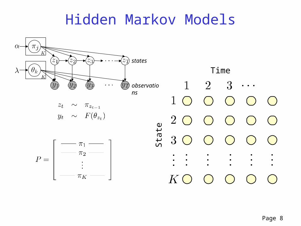
Hidden Markov Models
Time
Sta
te
states
observations
Page 9
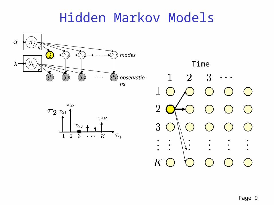
Hidden Markov Models
Timemodes
observations
Page 10
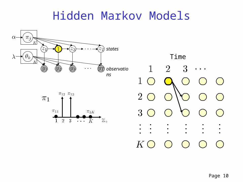
Hidden Markov Models
Timestates
observations
Page 11
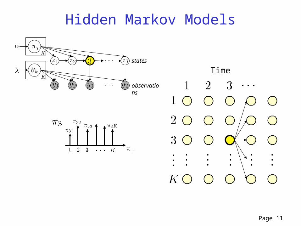
Hidden Markov Models
Timestates
observations

Issues with HMMs
• How many states should we use?– we don’t know the number of speakers a priori– we don’t know the number of behaviors a priori
• How can we structure the state space?– how to encode the notion that a particular time series makes
use of a particular subset of the states?– how to share states among time series?
• We’ll develop a Bayesian nonparametric approach to HMMs that solves these problems in a simple and general way

Bayesian Nonparametrics
• Replace distributions on finite-dimensional objects with distributions on infinite-dimensional objects such as function spaces, partitions and measure spaces– mathematically this simply means that we work with
stochastic processes
• A key construction: random measures
• These are often used to provide flexibility at the higher levels of Bayesian hierarchies:

Stick-Breaking
• A general way to obtain distributions on countably infinite spaces
• The classical example: Define an infinite sequence of beta random variables:
• And then define an infinite random sequence as follows:
• This can be viewed as breaking off portions of a stick:

Constructing Random Measures
• It's not hard to see that (wp1)• Now define the following object:
• where are independent draws from a distribution on some space
• Because , is a probability measure---it is a random measure
• The distribution of is known as a Dirichlet process:
• What exchangeable marginal distribution does this yield when integrated against in the De Finetti setup?

Chinese Restaurant Process (CRP)
• A random process in which customers sit down in a Chinese restaurant with an infinite number of tables– first customer sits at the first table
– th subsequent customer sits at a table drawn from the following distribution:
– where is the number of customers currently at table and where denotes the state of the restaurant after customers have been seated
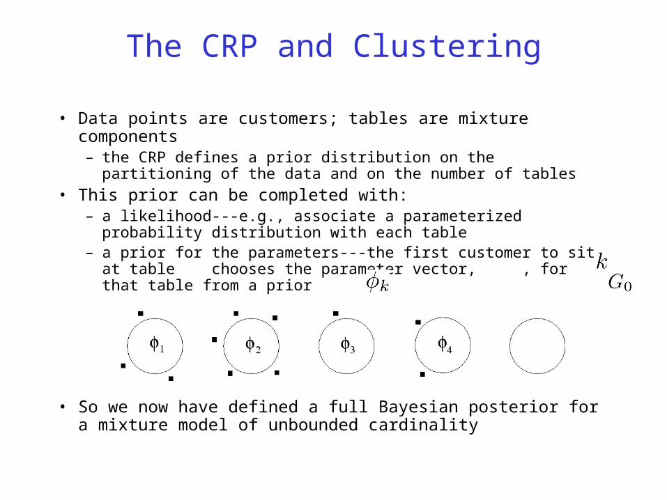
The CRP and Clustering
• Data points are customers; tables are mixture components– the CRP defines a prior distribution on the partitioning of the
data and on the number of tables
• This prior can be completed with:– a likelihood---e.g., associate a parameterized probability
distribution with each table– a prior for the parameters---the first customer to sit at table
chooses the parameter vector, , for that table from a prior
• So we now have defined a full Bayesian posterior for a mixture model of unbounded cardinality

CRP Prior, Gaussian Likelihood, Conjugate Prior

Dirichlet Process Mixture Models

Multiple estimation problems
• We often face multiple, related estimation problems
• E.g., multiple Gaussian means:
• Maximum likelihood:
• Maximum likelihood often doesn't work very well– want to “share statistical strength”

Hierarchical Bayesian Approach
• The Bayesian or empirical Bayesian solution is to view the parameters as random variables, related via an underlying variable
• Given this overall model, posterior inference yields shrinkage---the posterior mean for each combines data from all of the groups
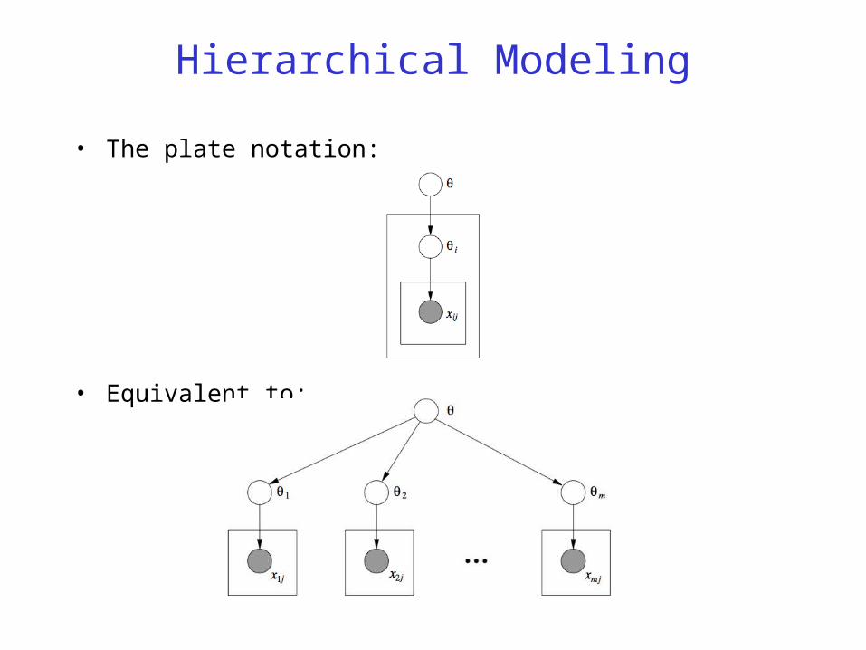
Hierarchical Modeling
• The plate notation:
• Equivalent to:

Hierarchical Dirichlet Process Mixtures(Teh, Jordan, Beal, & Blei, JASA 2006)

Marginal Probabilities
• First integrate out the , then integrate out

Chinese Restaurant Franchise (CRF)

Application: Protein Modeling
• A protein is a folded chain of amino acids
• The backbone of the chain has two degrees of freedom per amino acid (phi and psi angles)
• Empirical plots of phi and psi angles are called Ramachandran diagrams

Application: Protein Modeling
• We want to model the density in the Ramachandran diagram to provide an energy term for protein folding algorithms
• We actually have a linked set of Ramachandran diagrams, one for each amino acid neighborhood
• We thus have a linked set of density estimation problems
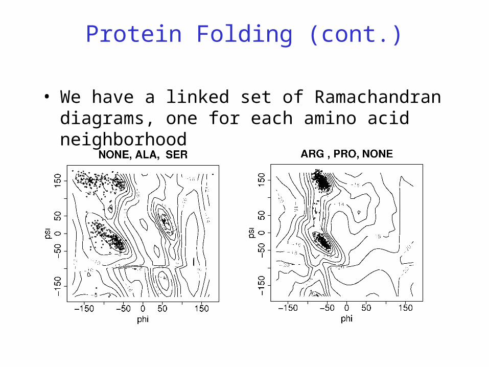
Protein Folding (cont.)
• We have a linked set of Ramachandran diagrams, one for each amino acid neighborhood

Protein Folding (cont.)

Nonparametric Hidden Markov models
• Essentially a dynamic mixture model in which the mixing proportion is a transition probability
• Use Bayesian nonparametric tools to allow the cardinality of the state space to be random– obtained from the Dirichlet process point of view (Teh,
et al, “HDP-HMM”)
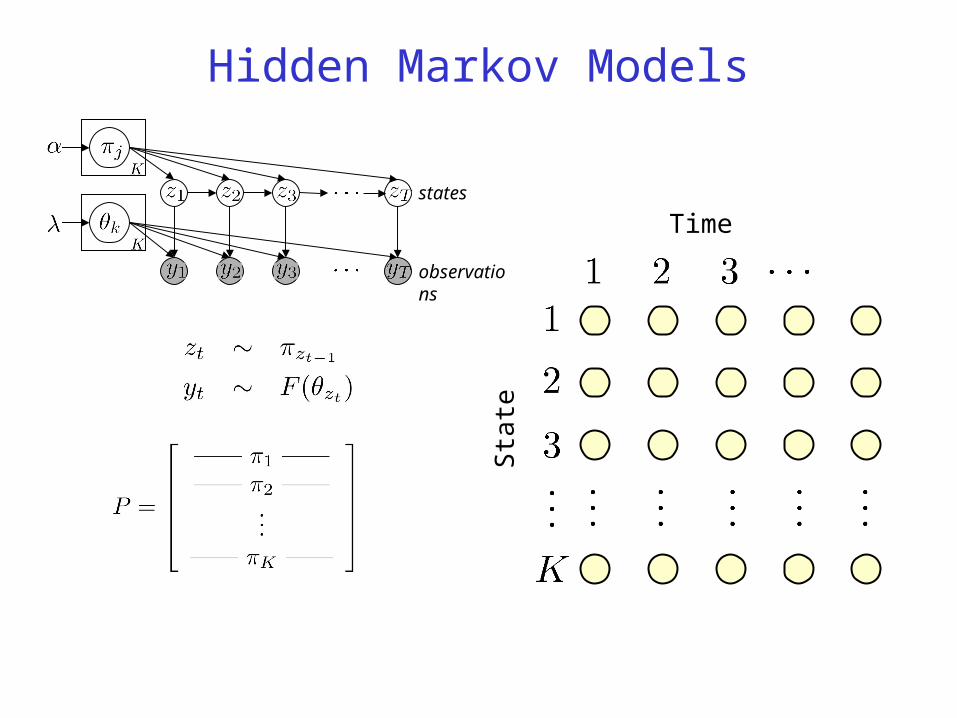
Hidden Markov Models
Time
Sta
te
states
observations
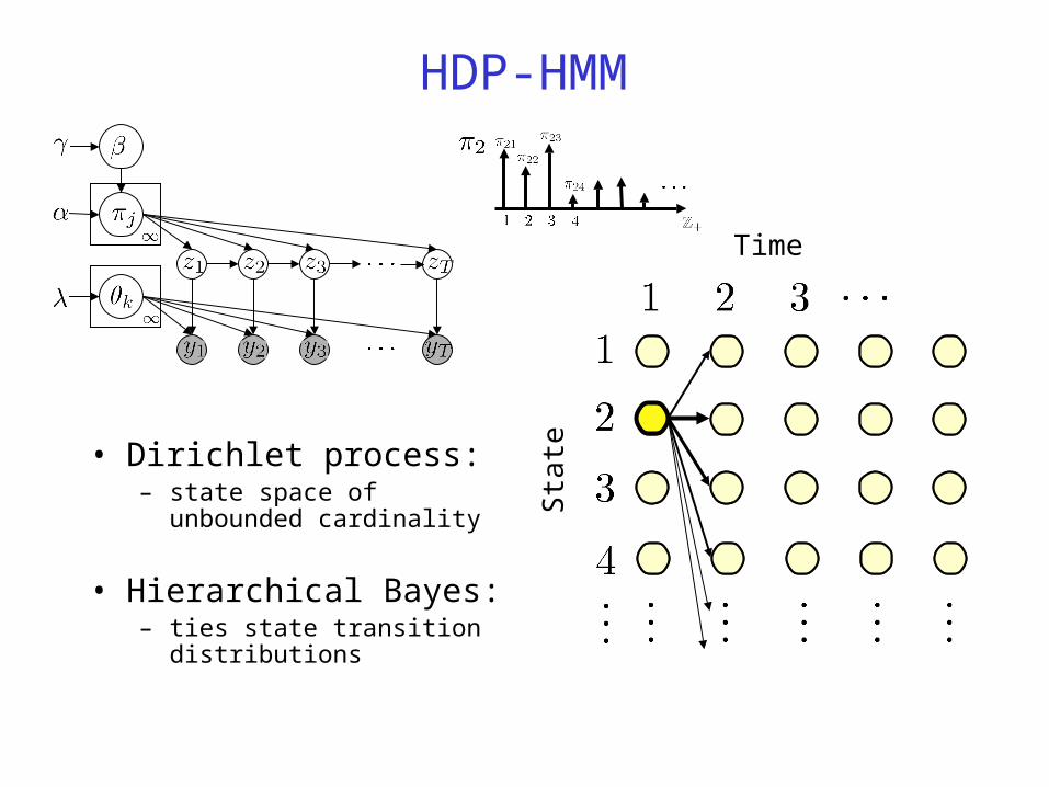
HDP-HMM
• Dirichlet process:– state space of unbounded
cardinality
• Hierarchical Bayes:– ties state transition
distributions
Time
Sta
te
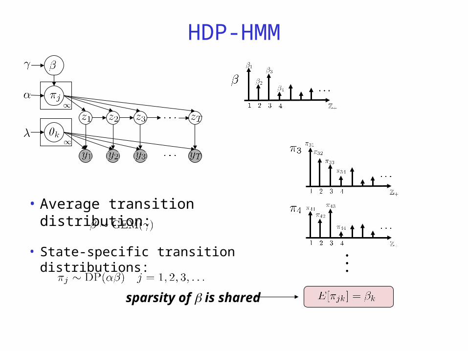
• Average transition distribution:
HDP-HMM
sparsity of is shared
• State-specific transition distributions:

State Splitting
• HDP-HMM inadequately models temporal persistence of states• DP bias insufficient to prevent unrealistically rapid dynamics• Reduces predictive performance
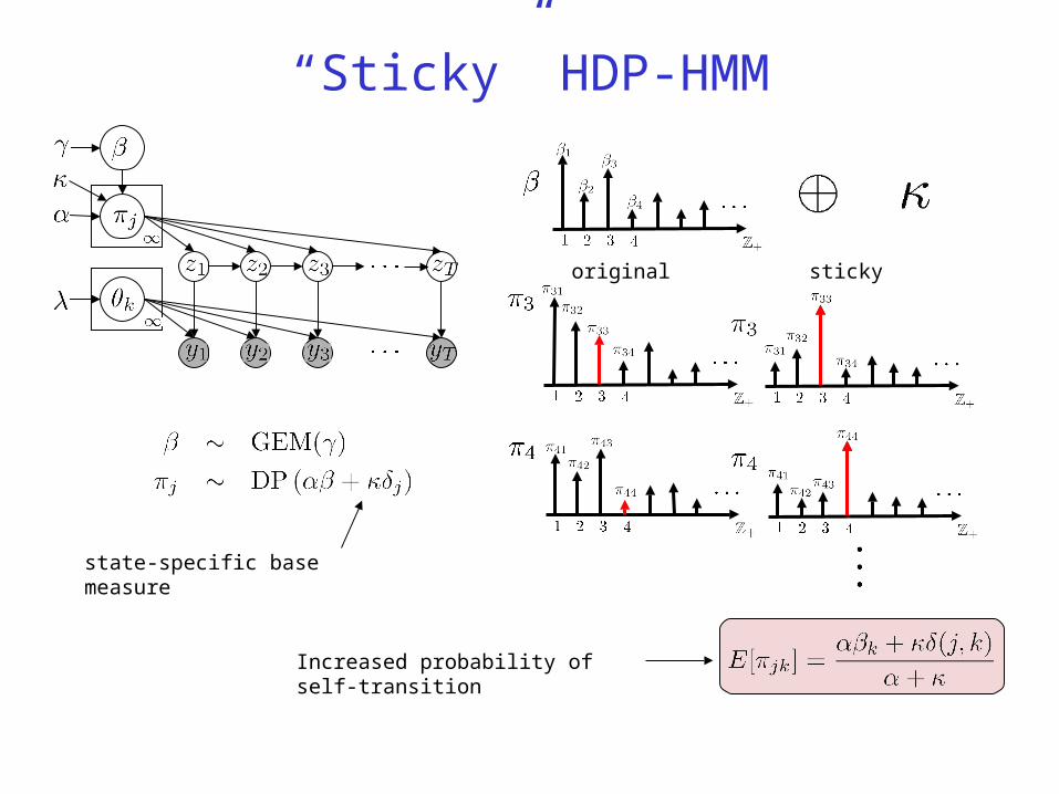
“Sticky” HDP-HMM
state-specific base measure
Increased probability of self-transition
original sticky

TIME50 100 150 200 250 300
John JaneBob JohnBob
Jill
0 1 2 3 4 5 6 7 8 9 10
x 104
-30
-20
-10
0
10
20
30
40
TIME
Speaker Diarization

NIST Evaluations
• NIST Rich Transcription 2004-2007 meeting recognition evaluations
• 21 meetings
• ICSI results have been the current state-of-the-art
Meeting by Meeting Comparison

Results: 21 meetings
Overall DER Best DER Worst DER
Sticky HDP-HMM 17.84% 1.26% 34.29%
Non-Sticky HDP-HMM 23.91% 6.26% 46.95%
ICSI 18.37% 4.39% 32.23%

Results: Meeting 1 (AMI_20041210-1052)
Sticky DER = 1.26%
ICSI DER = 7.56%

Results: Meeting 18 (VT_20050304-1300)
Sticky DER = 4.81%
ICSI DER = 22.00%
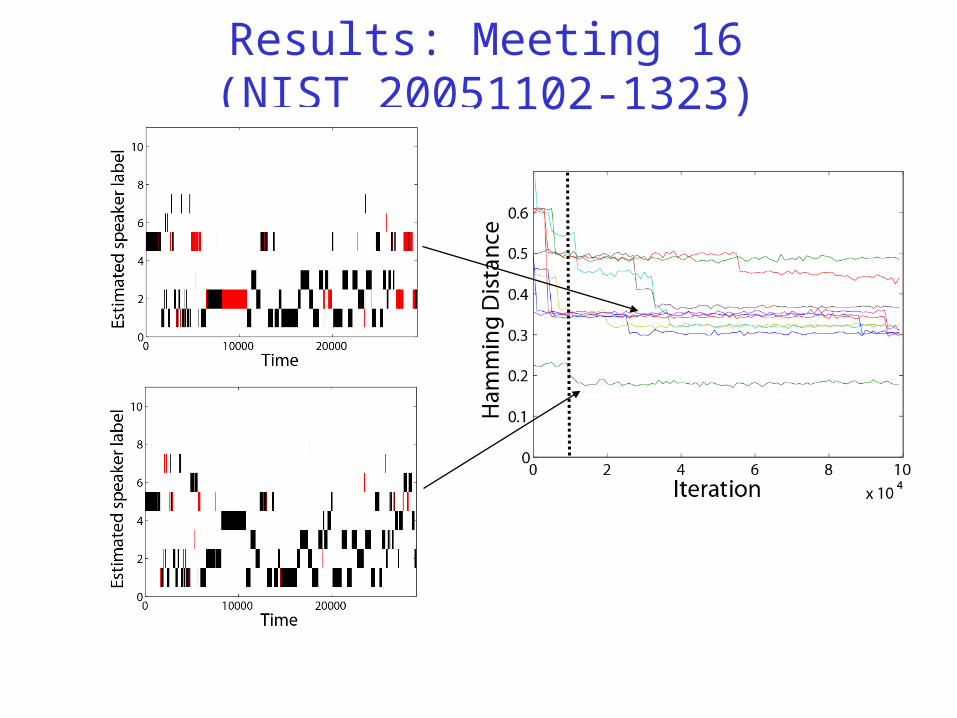
Results: Meeting 16 (NIST_20051102-1323)

The Beta Process
• The Dirichlet process naturally yields a multinomial random variable (which table is the customer sitting at?)
• Problem: in many problem domains we have a very large (combinatorial) number of possible tables– using the Dirichlet process means having a large
number of parameters, which may overfit
– perhaps instead want to characterize objects as collections of attributes (“sparse features”)?
– i.e., binary matrices with more than one 1 in each row

Completely Random Processes
• Completely random measures are measures on a set that assign independent mass to nonintersecting subsets of– e.g., Brownian motion, gamma processes, beta processes,
compound Poisson processes and limits thereof
• (The Dirichlet process is not a completely random process– but it's a normalized gamma process)
• Completely random processes are discrete wp1 (up to a possible deterministic continuous component)
• Completely random processes are random measures, not necessarily random probability measures
(Kingman, 1968)

Completely Random Processes
• Assigns independent mass to nonintersecting subsets of
(Kingman, 1968)
_
x
x
x
x
x
x
x
x
x
x
x
x
xx
x
! i
(! i ;pi )
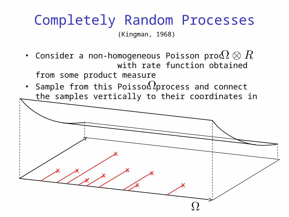
Completely Random Processes
• Consider a non-homogeneous Poisson process on with rate function obtained from some product measure
• Sample from this Poisson process and connect the samples vertically to their coordinates in
(Kingman, 1968)
R
xxx
xx
xx
x
x
(! i ;pi )
º

Beta Processes
• The product measure is called a Levy measure
• For the beta process, this measure lives on and is given as follows:
• And the resulting random measure can be written simply as:
(Hjort, Kim, et al.)
degenerate Beta(0,c) distribution Base measure

Beta Processes
p
!

Beta Process and Bernoulli Process

BP and BeP Sample Paths

Beta Process Marginals
• Theorem: The beta process is the De Finetti mixing measure underlying the a stochastic process on binary matrices known as the Indian buffet process (IBP)
(Thibaux & Jordan, 2007)

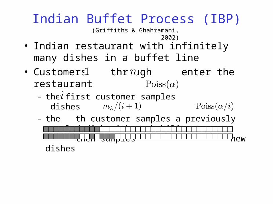
Indian Buffet Process (IBP)
• Indian restaurant with infinitely many dishes in a buffet line
• Customers through enter the restaurant– the first customer samples dishes
– the th customer samples a previously sampled dish with probability then samples new dishes
(Griffiths & Ghahramani, 2002)

Indian Buffet Process (IBP)
• Indian restaurant with infinitely many dishes in a buffet line
• Customers through enter the restaurant– the first customer samples dishes
– the th customer samples a previously sampled dish with probability then samples new dishes
(Griffiths & Ghahramani, 2002)
Indian Buffet Process (IBP)
• Indian restaurant with infinitely many dishes in a buffet line
• Customers through enter the restaurant– the first customer samples dishes
– the th customer samples a previously sampled dish with probability then samples new dishes
(Griffiths & Ghahramani, 2002)

Indian Buffet Process (IBP)
• Indian restaurant with infinitely many dishes in a buffet line
• Customers through enter the restaurant– the first customer samples dishes
– the th customer samples a previously sampled dish with probability then samples new dishes
(Griffiths & Ghahramani, 2002)

Indian Buffet Process (IBP)
• Indian restaurant with infinitely many dishes in a buffet line
• Customers through enter the restaurant– the first customer samples dishes
– the th customer samples a previously sampled dish with probability then samples new dishes
(Griffiths & Ghahramani, 2002)

Beta Process Point of View
• The IBP is usually derived by taking a finite limit of a process on a finite matrix
• But this leaves some issues somewhat obscured:– is the IBP exchangeable?– why the Poisson number of dishes in each row?– is the IBP conjugate to some stochastic process?
• These issues are clarified from the beta process point of view
• A draw from a beta process yields a countably infinite set of coin-tossing probabilities, and each draw from the Bernoulli process tosses these coins independently

Hierarchical Beta Processes
• A hierarchical beta process is a beta process whose base measure is itself random and drawn from a beta process

Multiple Time Series
• Goals:– transfer knowledge among related time series in the form of
a library of “behaviors”– allow each time series model to make use of an arbitrary
subset of the behaviors
• Method:– represent behaviors as states in a nonparametric HMM– use the beta/Bernoulli process to pick out subsets of states

IBP-AR-HMM• Bernoulli process
determines which states are used
• Beta process prior: – encourages sharing– allows variability

Motion Capture Results

Conclusions
• Hierarchical modeling has at least an important a role to play in Bayesian nonparametrics as is plays in classical Bayesian parametric modeling
• In particular, infinite-dimensional parameters can be controlled recursively via Bayesian nonparametric strategies
• For papers and more details:
www.cs.berkeley.edu/~jordan/publications.html