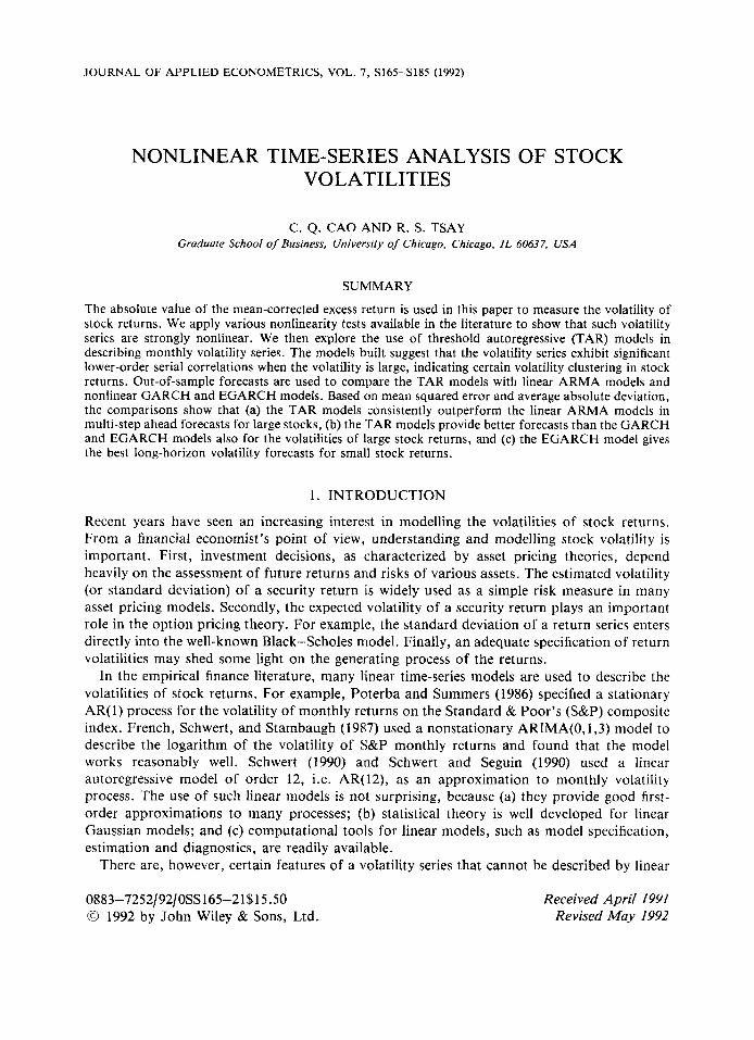
JOURNAL OF APPLIED ECONOMETRICS, VOL. 7 , S165-Sl85 (1992)

NONLINEAR TIME-SERIES ANALYSIS OF STOCK VOLATILITIES

C. Q . CAO AND R. S. TSAY Graduate School of Business, Univenity of Chicago, Chicago, IL 60637, USA

SUMMARY

The absolute value of the mean-corrected excess return is used in this paper to measure the volatility of stock returns. We apply various nonlinearity tests available in the literature to show that such volatility series are strongly nonlinear. We then explore the use of threshold autoregressive (TAR) models in describing monthly volatility series. The models built suggest that the volatility series exhibit significant lower-order serial correlations when the volatility is large, indicating certain volatility clustering in stock returns. Out-of-sample forecasts are used to compare the TAR models with linear ARMA models and nonlinear GARCH and EGARCH models. Based on mean squared error and average absolute deviation, the comparisons show that (a) the TAR models consistently outperform the linear ARMA models in multi-step ahead forecasts for large stocks, (b) the TAR models provide better forecasts than the GARCH and EGARCH models also for the volatilities of large stock returns, and (c) the EGARCH model gives the best long-horizon volatility forecasts for small stock returns.

1. INTRODUCTION

Recent years have seen an increasing interest in modelling the volatilities of stock returns. From a financial economist’s point of view, understanding and modelling stock volatility is important. First, investment decisions, as characterized by asset pricing theories, depend heavily on the assessment of future returns and risks of various assets. The estimated volatility (or standard deviation) of a security return IS widely used as a simple risk measure in many asset pricing models. Secondly, the expected volatility of a security return plays an important role in the option pricing theory. For example, the standard deviation of a return series enters directly into the well-known Black-Scholes model. Finally, an adequate specification of return volatilities may shed some light on the generating process of the returns.

In the empirical finance literature, many linear time-series models are used to describe the volatilities of stock returns. For example, Poterba and Summers (1986) specified a stationary AR( 1) process for the volatility of monthly returns on the Standard & Poor’s (S&P) composite index. French, Schwert, and Stambaugh (1987) used a nonstationary ARIMA(O,1,3) model to describe the logarithm of the volatility of S&P monthly returns and found that the model works reasonably well. Schwert (1990) and Schwert and Seguin (1990) used a linear autoregressive model of order 12, i.e. AR(12), as an approximation to monthly volatility process. The use of such linear models is not surprising, because (a) they provide good first- order approximations to many processes; (b) statistical theory is well developed for linear Gaussian models; and (c) computational tools for linear models, such as model specification, estimation and diagnostics, are readily available.

There are, however, certain features of a volatility series that cannot be described by linear

0883-7252/92/0SS165-21$15.50 0 1992 by John Wiley & Sons, Ltd.

Received April 1991 Revised May 1992

S166 C. 0. CAO AND R. S. TSAY

time series models. For instance, empirical evidence shows that stock returns tend to exhibit clusters of outliers, implying that the volatility series evolves over time in a nonlinear fashion. Such limitations of linear models have motivated many authors to consider nonlinear alternatives. See, for example, Gallant, Hsieh, and Tauchen (1991), Hsieh (1989), LeBaron (1992), Scheinkman and LeBaron (1989), Pagan and Schwert (1990), and Taylor (1986).

The most commonly used nonlinear time-series models in the finance literature are the autoregressive conditional heteroscedastic (ARCH) model of Engle (1982), the generalized ARCH (GARCH) model of Bollerslev (1986) and the exponential GARCH (EGARCH) model of Nelson (1991). These ARCH-family models have been found to be useful in capturing certain nonlinear features of financial time-series. In particular they are capable of producing heavy-tailed distributions and clusters of outliers. See Bollerslev, Chou, and Kroner (1992) for a nice review of these models and their applications. The success of the ARCH-type of models is understandable if we consider their relation to the random-coefficient autoregressive (RCA) models that, to a certain degree, are adaptive to the changing economical environment. As pointed out by Tsay (1987), a RCA model can produce, under some mild conditions, the first two conditional moments of an ARCH model. This is particularly so under the normality assumption.

The ARCH-family is only one of many time-series models that can capture the nonlinear characteristics of stock volatilities commonly observed in practice. The purpose of this paper is, therefore, to explore some other nonlinear models and to compare their forecasting accuracy with those of ARCH-family models. More specifically we have two goals. First, we consider directly a volatility process for a monthly stock return and test the nonlinearity of such a volatility process. Secondly, in the presence of nonlinearity, we address the issue of modelling the volatility process via a piecewise linear model and then compare the forecasts of such a model with those of GARCH and EGARCH models. The piecewise linear model employed is the threshold autoregressive model, (see Tong, 1990). The use of such models is motivated by their ability to capture the asymmetric pattern of a time-series and by their local linear property. We adopt the common belief that all statistical models are wrong, but a well- chosen one can provide accurate local approximations.

This paper is organized as follows. In section 2 we briefly introduce the three nonlinear models and the nonlinearity tests used in the paper. A modelling procedure for the TAR models is also given. Section 3 describes the data employed. For a monthly stock process the absolute value of its excess return minus the mean, pre-multiplied by &/2), is used to obtain a volatility series. This definition is based on the fact that 4 ~ / 2 ) I R , - pf 1 is an unbiased estimator for the conditional standard deviation (volatility) of the monthly excess returns if the excess return R , is normally distributed. We then apply in section 4 the nonlinearity tests of section 2 to the constructed volatility series. In section 5 we apply the TAR models to three volatility series of monthly stock returns. Finally, in section 6 we compare the TAR models with linear ARMA models and nonlinear GARCH and EGARCH models via out-of-sample forecasts.

2. NONLINEAR MODELS AND NONLINEARITY TESTS

2.1. Some Nonlinear Dynamic Models

Many nonlinear time-series models are available in the literature. Tong (1990) gives a nice summary of those models. Here we briefly discuss the three models employed in this paper.

STOCK VOLATILITIES S167

A time series Yr follows a GARCH(p,g) model if it satisfies:

Yt = Xrb + (1)

where X I is a vector of explanatory variables including possibly lagged values of Yt, b is a constant vector and the error term Et is given by

P

~t = atzt, Z r - i.i.d. N(0, I ) , a: = a0 + 2 + p j ~ : - j (2) r = l J = 1

where p and q are nonnegative integers, LYO > 0, at 2 0 for i > 0 and P, 2 0 for all j . If (EY= 1 a, + C:=, pJ) < 1, the innovational process ( E ~ ] of (1) is weakly stationary. For the most commonly used GARCH(1,l) model, the condition 3a f + 2a1P1 + p: < 1 implies the existence of the fourth moment of E j , which is greater than that of a normal random variable. Con- sequently, the GARCH model is capable of producing outliers. The non-negative constraints on the coefficients a, and P, of a,? for i > 0 and J 2 0 in (2) can be relaxed (see Tsay, 1987 and Nelson and Cao, 1992 for details). For furl her properties of the GARCH models see Engle ( 1982) and Bollerslev (1 986).

The key feature of the GARCH model is that, by equation (2) , the conditional variance of is predictable. Replacing &, of the variance equation in (2) by z ~ - , a ~ - , , we see that a large

conditional variance tends to be followed by another large conditional variance. This feature implies that the GARCH model is capable of producing clusters of outliers. In financial time- series, clusters of outliers result in clusters of high volatilities.

A limitation of the GARCH model is thal the conditional variance a,? responds to positive and negative residuals e l - , in the same manner. On the contrary, empirical evidence in financial time-series shows that there is a negative correlation between the current returns and future returns volatility. To overcome such a limitation, Nelson (1991) proposed an exponential- CARCH model, which enables the conditional variance of the innovation to respond asymmetrically to positive and negative residuals. A time-series Yl follows an EGARCH(p, q ) model if it satisfies

Y t = X t b + ~ r , Er=orZ r , Zr-i.i.d. N(O,l),

1 + a i B + +2B2 + ... + aqBq In a,? = a + g(zr- 1 ) 1 - A I B - A2B2 - ... - ApBP

(3)

where g(Zr) = 0Zr + y[ zt 1 - E 1 zr 1 1 , B is the lag operator, @;, Aj, 0, and y are parameters such that the two polynomials (1 + Cy=1 aJ3') and (1 - Cy==, AjBj ) have no common factors. Consider the g ( z t ) function above. If Zr is positive then g(zt) is a linear function of Zr with slope (0 + y). I f zt is negative then the slope changes to (0 - y). Consequently, the conditional variance a: responds asymmetrically to the sign of the innovation Zr-c.

A time-series Yr is a TAR process if it satisfies the model

Yt=+6"++1("Yr-1 +.-. + + J ' ) Y ~ - ~ + E / ' ) if Yr-dEL;, i = 1,2, ..., k (4)

where the L; form a non-overlapping partition of the real line i.e. U f= IL; = R and L, n LJ = 0 if i # j , k is the number of threshold regimes, d is the delay parameter (or threshold lag), p is the AR order and ( E / ' ) ) is a sequence of i.i.d. normal random variables with mean zero and variance of such that ( c / " ) and (ct(j)) are independent if i # j . The TAR model in (4) is a piecewise linear model in the space of Yl-d and is capable of providing accurate 'local approximations' in this space. It is, however, not a piecewise linear model in time. The key features of TAR models include time-irreversibility, asymmetric limit cycle and jump phenomenon. See Tong (1990) for other properties of TAR Models.

S168 C . Q. CAO AND R. S. TSAY

Alternatively, one can interpret a TAR model as a switching linear regression model for which many references are available in the literature. See, for example, Quandt and Ramsey (1978). The only difference is that for the TAR model in (4), the switching mechanism is controlled by the threshold variable Y,-d, not by the time index 1.

The idea of using a threshold variable Yt-d to govern the dynamic pattern of a stock volatility series Y, appears to be natural. As mentioned before, empirical evidence suggests that large returns tend to be followed by large returns and small returns by small returns. This evidence shows, among other possibilities, that the dynamic pattern of stock volatilities evolves with the past values of the returns. Such a state-dependent evolution is in good agreement with the concept of TAR models.

2.2. A Modelling Procedure for TAR Models

The modelling of GARCH and EGARCH processes has been discussed in the econometrics literature. For TAR models we shall use the modelling procedure of Tsay (1989, 1991). The main idea of the procedure is to transform a TAR model into a regular change-point problem in linear regression analysis. This is achieved by using the concepts of 'arranged autoregression' and 'local estimation'. Here local estimation means that we perform a sequential estimation with a fixed-length window that controls the number of observations used. However, instead of using the time index, arranged autoregression uses the magnitude of the threshold variable Yr-d to control the data flow of the window. By so doing we effectively transform the threshold problem into a switching regression problem for which statistics can be derived to test for model changes and to explore the dynamic structure of the process. For illustration, Part (a) of the Table I shows the usual set-up of fitting an AR(2) model to 10 consecutive observations of the TAR(2) model

l.3Yt-1 - 0 . 4 Y r - 2 + ~ , ( 1 ) if Y , - 2 < 0 - 0 0.3Yr- 1 + O.4Yr-2 + E,(') otherwise, Y,= [

where c,(') are independent sequences of i.i.d. N(0, 1) random variates, L.1 = ( - a, 0) and LZ = [0, m). Obviously, such a set-up cannot yield consistent parameter estimates. On the other hand an arranged autoregression rearranges the set-up into that of Part (b) based on the magnitude of the threshold variable Yt -2 . It is then clear that in this particular instance the first four rows belong in the first regime of the TAR(2) model, whereas the last four rows belong in the second regime. A local estimation can thus provide consistent estimates of the

Table I

(a) Ordinary autoregression (b) Arranged autoregression ~ ~~

Time Y/ Y/- I Yr-2 regime Time

3 -0.41 1.21 1.31 L 2

4 0.21 -0.41 1.21 L2

5 - 1-12 0.21 -0 -41 Ll

6 -3.08 -1.12 0.21 L 2

7 - 1 . 8 5 -3.08 -1.12 LI 8 0.12 - 1 . 8 5 -3.08 LI 9 0-58 0.12 - 1 . 8 5 LI

10 1.28 0.58 0.12 L 2

8 9 7 5

10 6 4 3

Y/ y / - I Yt-2 regime

0.12 - 1 . 8 5 -3.08 L\ 0.58 0.12 -1'8.5 Li

-1.85 - 3 . 0 8 - 1.12 LI - 1.12 0.21 -0 .41 LI

1.28 0.58 0.12 L2 -3.08 -1.12 0.21 L2

0.21 -0.41 1.21 L2 -0 .41 1.21 1.31 L2

STOCK VOLATII.ITIES S169

coefficients. In particular, the local estimates should be stable before the first change point enters the estimation window. In practice the local estimation can be done efficiently by a recursive least-squares algorithm or Kalman filter; the latter is particularly useful when there are missing values in the data.

We then consider the scatterplots of the local estimates of AR coefficients versus the threshold variable YI-d. Ideally, the scatterplots should look like a step function with jumps indicating the values of the threshold variable at which the regime changes. In practice, since the windows used overlap sequentially, the plots tend to show certain smooth transition from one regime to another. This is not a serious problem in model specification, because the main objective of arranged autoregression is to provide information on the possible partitions of the space of the threshold variable. Once the threshold values are located we can partition the space into several regimes and estimate an AR model with an appropriate order in each regime. Furthermore, we can adjust the threshold values to refine the estimated TAR model according to some information criterion, e.g. the AIC: criterion.

In summary, the TAR modelling procedure used consists of the following steps:

1 .

2.

3. 4. 5. 6.

Select a tentative AR order p and a set of possible threshold variables. In this paper the possible threshold lags entertained are (1,2, ..., 12). For each threshold variable considered, perform nonlinearity tests, especially a threshold nonlinear test. Select the threshold variable Yl-d based on the test results of step 2. Perform an arranged autoregression to locate the possible threshold values. Estimate the specified TAR model by conditional least-squares. Check the estimated TAR model and refine it if necessary.

See Tsay (1989) for details and examples of such a procedure. It is worth mentioning that the computation of the above procedure is extremely simple. It merely requires a sorting routine and a recursive least-squares algorithm.

2.3. Some Nonlinearity Tests

To detect the nonlinearity of a stock volatility in section 4 we apply some nonlinearity tests available in the literature. The tests used include the F-test of Tsay (1986), the augmented F-test of Luukkonen, Saikkonen, and Terasvirta (1988), the threshold test of Tsay (1989) and a general nonlinearity test of Tsay (1991). For model checking we use the BDS test of Brock, Dechert, and Scheinkman (1987) to tesl the i.i.d. assumption of the residuals. For completeness we briefly describe these tests in this subsection.

The F-test is a Lagrange multiplier test for detecting mainly second-order nonlinearity in an AR model. For a time series Yt with observations ( Y 1 , Y2, ..., YT) , the test consists of three steps: (1) For a prespecified AR order p, regress Y, on the vector Wf = (1, Yt- ..., Y, - , ) , and compute the residual cil. (2) Regress the vector of squares and cross-products of Z , - , , i.e., Z / = ( Y : - 1 , Y , - I Y ~ - z ,..., Y ~ - I Y / - ~ , Yr-2, Y,-2YI-3 ..., Yf- , ) , on W, and save the residual vector vr. (3) Regress cir on vr and calculate the residual &. Form the F-statistic

2

- (C P/ci/)(C P;P/)-l(C P;a,)/m F = C 2.?/(T- p - I?? - 1)

where m = i p ( p + 1) and the summation is summing over t from p + 1 to T. It can be shown that, under the null hypothesis that the ( Y , ) is a stationary AR(p) process, P i s asymptotically an F distribution with degrees of freedom ,! p ( p + 1) and T - $ p ( p + 3) - 1 .

S170 C . Q. CAO AND R. S . TSAY

Luukkonen, Saikkonen, and Terasvirta (1988) modified the above F-test by augmenting to the vector Zt the cubic terms Y;- I , Yt-2 , ..., Y:-p. These authors show via simulation that such an augmented-F-test is more powerful than the original F-test in detecting certain types of nonlinear models, e.g. the logistic model.

To detect the threshold nonlinearity, Tsay (1989) proposed another F-test based on the arranged autoregression. The test consists of two steps. First, for a prespecified AR order p and a threshold lag d, fit recursively an arranged autoregression of order p to the series Y,. Assuming that the recursion begins with the first b observations, calculate the standardized predictive residual Pt for t > b. Secondly, regress the predictive residual Pt on (1, Y t - , , Y t -2 , ..., Y t - p ) , save the corresponding residuals &, and form the F-statistic

3

where h = max(1,p + 1 - d ) and the summation is summing over t from b + 1 to T - d - h + 1. Under the null hypothesis that Yt is an AR(p) process, the P(p, d ) statistic is asymptotically an F distribution with degrees of freedom p + 1 and T - d - b - p - h.

The general nonlinearity test of Tsay (1991) combines the ideas of the threshold test and F-tests. It is a test designed for detecting various types of nonlinearity. Similar to the threshold test, one computes first the predictive residual Pt of an arranged autoregression of order p and threshold lag d. Next, one regresses Ct on the regressors (1, Y t - l , ..., Y1-,,), ( Y ~ - I & ~ , ..., ~ ~ - ~ e ~ - ~ ) , (et-let-2, . . . ,et-per-p-l) , ( ~ ~ - 1 exp(- ~ ? - l / r ) , + ( z t - d ) , Y , - 1 + ( z l - d ) ) ,

where r = maxt I Yt - I I and Zt-d = ( r l - d - yd) /Sd with Y d and Sd the sample mean and standard deviation of Yl-d, @( - ) is the cumulative distribution function of the standard normal random variable. The usual F-statistic of this second regression is the test statistic, which under the null hypothesis of an AR(p) model for Yt follows asymptotically an F- distribution with degrees of freedom 3 ( p + 1) and T - b - 3(p + I), where b is defined as before.

The BDS test of Brock, Dechert, and Scheinkman (1987) is based on the idea of correlation dimension. It is a useful statistic for detecting i.i.d. random samples. Define an rn-dimensional vector YY = (Yt , Y,, I , ..., Yt+,,- I ) . Then the sample correlation dimension of this m-vector is:

1 1 . . A

where 1 if 1 1 Y:"- Yf"I) < E

0 if ( 1 Y:" - YP 11 2 E , I,(Y:", Y f " ) =

with 1 1 - 1 1 the sup-norm. This correlation dimension measures the spatial correlation of the data. More precisely, the correlation dimension estimates the probability that any two rn-dimensional vectors, say Y;" and Y f " , are within the distance c. Under the null hypothesis that the [ Y t ) are i.i.d. with a nondegenerated density function f( ), the BDS-U statistic

J7Kir (c ) - (Cl (f ))"'I u;,, = um (f 1

is asymptotically N(0, l), where

STOCK VOLATILITIES S171

In our implementation of the BDS-U statistic we use m = 2, ..., 5 and E = 1 ,1*5 and 2 times the standard deviation of Y,. These choices are based on suggestions of Hsieh and LeBaron ( 1 988).

3. DATA DESCRIPTION

3.1. Stock Return Series

The stock returns used in this paper are the rnonthly value-weighted, equal-weighted and S&P composite portfolio excess returns for NYSE: & AMEX for the period from January 1928 to December 1989. The data are from the Center for Research in Security Prices (CRSP) at the University of Chicago and have 744 observations. We also use daily returns of these three stocks from 1985 to 1989 to construct benchmark series of monthly stock volatilities for model comparisons in section 6 . A return series is defined as the logarithm of the price relative, which is the continuously compounded rate of return. Monthly excess return is simply the above stock return less the 1-month Treasury-bill return.

3.2. Volatility Series of Stock Returns

Following Schwert (1990) and Schwert and Seguin (1990), we use in this paper the absolute value of monthly excess return minus its mean, pre-multiplied by m) to estimate the volatility of monthly stock returns. In other words the volatility series used is a[ = m) I Rr - pt I for the monthly excess return Rt. For value-weighted and equal- weighted portfolio excess returns Rt - p t is taken as the residual of the AR(1) process for the excess returns. This is motivated by the fact that the AR(1) coefficients in the mean equation of the simple GARCH(1,I) and EGARCH(I,O) models are significant at the 5 per cent level for both excess return series. For S&P excess return, since the AR(1) specification in the mean equation of the GARCH(1,l) model is not statistically significant, the mean series pi is treated as a constant and estimated by the sample mean of R,.

3.3. Power Transformation

Since the distribution of the volatility measure is skewed, we consider its Box-Cox transformation

a:- 1 y, =z - X ’

to increase the efficiency of parameter estimation and to aid the model interpretation. It turns out that the distribution of Yr is fairly symmetric when X = t .

Alternatively, many authors in the literature modeled the logarithms of the volatility series Or, i.e. considering In(ar). See, for example, Poterba and Summers (1987), French, Schwert, and Stambough (1987), Melino and Turnbull (1990), Scott (1987), Stein (1989), and Wiggins (1987). For the volatility series = m2) I Rr - pr 1 , the distribution of In(u,) is not symmetric and the normality assumption is questionable. Table I1 gives some summary statistics of at, ln(at) and the transformed series Yr for the 3-monthly return series considered in the paper. From the table it is seen that the Box-Cox transformed series Yr is much closer to normality than a, and In(a,) series are.

S172 C. Q. CAO AND R. S. TSAY

Table 11. Summary statistics of volatility, logarithm of volatility and transformed volatility of S&P, value-weighted and equal-weighted excess returns, 1928- 1989

S&P VW EW

In ul

Mean 0.0505 Variance 0.0030 Skewness 3.2692 Kurtosis 18.7543 Minimum 0.0000 Median 0.0371 Maximum 0.4476

~ 3.5136 1.4680

- 1.3245 7.0134

- 11.5129 - 3.2938 -0.8037

Yl

-2.2690 0.2108 0.0106 3 .4924

-3.7751 -2.2444 -0.7281

Yl UI In uI Yl

0.0495 -3.5111 0.0027 1.3582

16.8344 5.2033 3.0303 - 1.0863

0.0001 - 9.6979 0.0361 - 3.3207 0.4349 -0.8327

- 2.2719 0.2016

- 0.0006 3.3495

- 3.6459 -2.2561 - 0.75 I8

0.0634 0.0050 3.0349

15.8402 0~0000 0.0419 0.5488

-3.3161 -2.1773 1.5410 0.2478

- 1.2315 0.0657 6.2693 3-4188

-10.7534 -3.7280 -3.1723 -2.1902 -0.6001 -0.5573

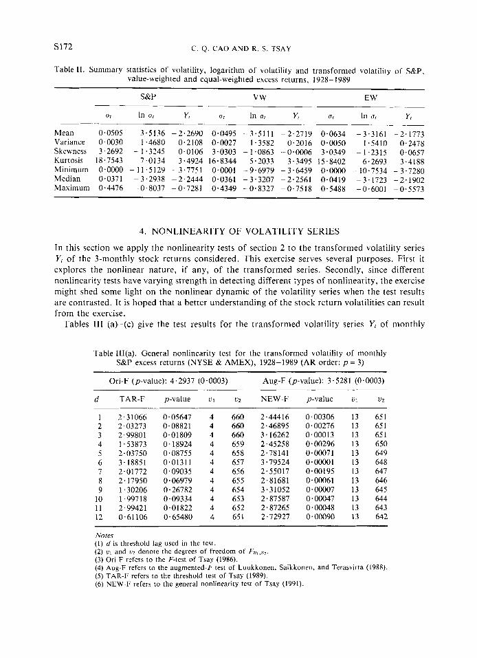
4. NONLINEARITY OF VOLATILITY SERIES

In this section we apply the nonlinearity tests of section 2 to the transformed volatility series Yt of the 3-monthly stock returns considered. This exercise serves several purposes. First it explores the nonlinear nature, i f any, of the transformed series. Secondly, since different nonlinearity tests have varying strength in detecting different types of nonlinearity, the exercise might shed some light on the nonlinear dynamic of the volatility series when the test results are contrasted. It is hoped that a better understanding of the stock return volatilities can result from the exercise.

Tables 111 (a)-(c) give the test results for the transformed volatility series Y, of monthly

Table III(a). General nonlinearity test for the transformed volatility of monthly S&P excess returns (NYSE & AMEX), 1928-1989 (AR order: p = 3)

Ori-F (p-value): 4.2937 (0.0003) Aug-F (p-value): 3.5281 (0.0003)

d TAR-F p-value V I u2 NEW-F p-value u1 u2

1 2.31066 0.05647 4 660 2.44416 0.00306 13 651 2 2.03273 0-08821 4 660 2.46895 0.00276 13 651 3 2.99801 0.01809 4 660 3.16262 0.00013 13 651 4 1.53873 0.18924 4 659 2.45258 0.00296 13 650 5 2.03750 0.08755 4 658 2.78141 0-00071 13 649 6 3.18851 0.01311 4 657 3.79524 0.00001 13 648 7 2.01772 0.09035 4 656 2.55017 0.00195 13 647 8 2.17950 0.06979 4 655 2.81681 0.00061 13 646 9 1.30206 0.26782 4 654 3.31052 0.00007 13 645

10 1.99718 0.09334 4 653 2.87587 0-00047 13 644 1 1 2.99421 0-01822 4 652 2.87265 0.00048 13 643 12 0-61106 0-65480 4 651 2-72927 0.00090 13 642

Notes (1) d is threshold lag used in the test. (2) u , and u2 denote the degrees of freedom of FQ,~,, . (3) Ori-F refers to the F-test of Tsay (1986). (4) Aug-F refers to the augmented-F test of Luukkonen, Saikkonen, and Terasvirta (1988). (5) TAR-F refers to the threshold test of Tsay (1989). (6) NEW-F refers to the general nonlinearity test of Tsay (1991).

STOCK VOLATILITIES s173

Table III(b). General nonlinearity test for the transformed volatility of monthly value-weighted portfolio excess returns (NYSE & AMEX), 1928- 1989 (AR order: P = 3 )

Ori-F (p-value): 7.1646 (0.0000) Aug-F (p-value): 5.4901 (0.0000)

d TAR-F p-value V I u2 NEW-F p-value u1 u2

-

1 4.47796 0.00141 4 660 2-76723 0.00076 13 651 2 1.94288 0.10167 4 660 2.80423 0-00064 13 651 3 4.73253 0.00090 4 660 3.44988 0.00003 13 651 4 0.52882 0.71460 4 659 2.36994 0.00419 13 650 5 3.07864 0.01579 4 658 3.47296 0.00003 13 649 6 0.54480 0.70289 4 657 2.75708 0-00079 13 648 7 5.34855 0.00030 4 656 3.42249 0.00004 13 647 8 0.60031 0.66254 4 655 2.50549 0.00237 13 646 9 1.78051 0.13099 4 654 3.87354 0.00000 13 645

10 3.07780 0.01582 4 653 2.97072 0.00031 13 644 1 1 2-39830 0.04897 4 652 3-52244 0.00002 13 643 12 0.85416 0.49124 4 651 3-13386 0.00015 13 642

Table III(c). General nonlinearity test for the transformed volatility of monthly equal-weighted portfolio excess returns (NYSE & AMEX), 1928- 1989 (AR order: P = 4 )

Ori-F (p-value): 2.3813 (0.0089) Aug-F (p-value): 2.5232 (0.0016)

d

1 2 3 4 5 6 7 8 9

10 11 12

__ TAR-F

2.74321 2.04864 2.01 140 0.89265 1.36919 1.77481 1 . I7578 0-39319 2.39319 2.39532 1.25899 0.91282

p-value

0.01832 0.070 10 0.07514 0.48548 0.23391 0.11585 0 * 3 1947 0.85362 0.03640 0.03625 0.28000 0.47208

UI u2

5 657 5 657 5 657 5 657 5 656 5 655 5 654 5 653 5 652 5 651 5 650 5 649

NEW-F

1.62865 2 - 14205 2.1 I350 2.06468 1 . 8 I744 2.85989 2.2198 1 2.30309 2.39850 1 .87675 2.07094 2.53350

p-value

0.05659 0.00586 0.00671 0.00844 0.02568 0.000 16 0.00404 0.00270 0.00 168 0.01983 0.0082 I 0.00085

UI

16 16 16 16 16 16 16 16 16 16 16 16

u2

646 646 646 646 645 644 643 642 64 1 640 639 63 8

~

S&P, value-weighted and equal-weighted composite portfolio excess returns. For the S&P excess returns and value-weighted returns we use an AR order p = 3 in the tests and the null hypothesis is that Yl is a linear AR(3) process. For equal-weighted excess return p = 4 is used. These AR orders are determined by the partial autocorrelations of the Y, series. From the tables we observe that (a) the F-test and augmented-F-test suggest that all three transformed volatility series are nonlinear at the 1 per cent level; (b) the threshold test and the general test indicate that the series exhibit certain threshold nonlinearity, especially when d = 1 or 3; (c) the results show that the three volatility series do not have a unified nonlinear pattern. In summary the tests suggest that the transformed volatility series Yl are nonlinear and the TAR model might be able to capture some nonlinear characteristics of the series.

s174 C. Q . CAO AND R. S . TSAY

5. MODELLING THE VOLATILITY OF STOCK RETURNS

5.1. TAR Models for the Volatility Series

Based on the results of nonlinearity tests we build in this section TAR models for the three transformed volatility series. Consider first the monthly S&P excess returns. Following the modelling procedure of Section 2 we begin with the determination of the threshold variable d. To this end Table III(a) suggests that Yr-1, Y,-3, Y,-6 and Y f - l l are possible threshold variables, because they correspond to the most significant testing results. Since d = 6 or 11 is hard to interpret, we focus on the first two possible values. Further analysis of the estimation results led us to choose d = 1. In practice, if necessary, one can build a TAR model for each possible value of d and make a decision based on the models built. For instance, in this particular example one can build a TAR model for d = 1 and another model for d = 3, and make a decision between these two TAR models by using a model selection criterion such as the AIC criterion.

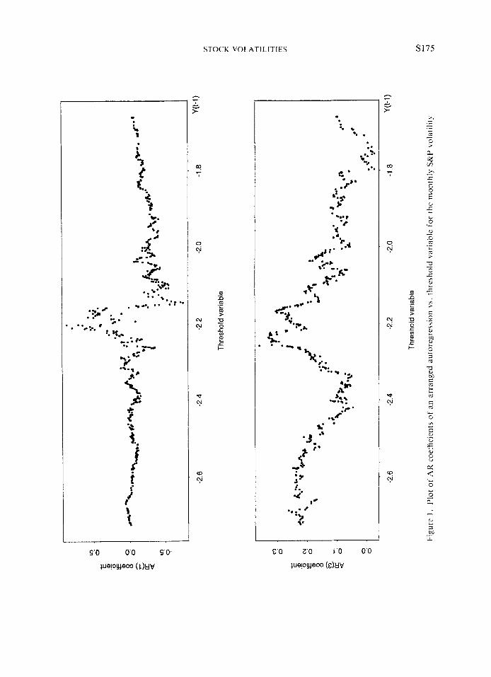
With d = 1 we turn to the specification of possible threshold values and, hence, the partition of the Yr-I space. Figure 1 shows the scatterplots of local estimates of AR-1 and AR-3 coefficients versus the threshold variable Y,-1. The local estimates are based on an arranged autoregression of order 3 with d = 1 and a window size 120. By window size we mean the number of observations used in the local estimation, which is done recursively by adding a new observation and deleting an old one in each iteration. From the scatterplots, especially the one of AR-I coefficient, the local estimates are relatively stable before and after Y,-l = -2.2, suggesting that there is a change point around Y , - I = -2 -2 . Consequently, we tentatively specify a two-regime TAR(3) model with a threshold YI- I = - 2.2 for the volatility series of the monthly S&P excess returns.

Finally, we refine the specification of the threshold value by searching through the neighbourhood of Y r - I = -2 .2 and using AIC as the selection criterion. I t turns out that Y r - I = - 2.16 provides a two-regime TAR(3) model with the minimum AIC. With such a model specification, we obtain the model:

q 5 h 1 ) + 4 f 1 ) Y r - l + 4 I 1 ) Y t - 2 + 4 j ' ) Y , - ~ + & , ( ' ) i f Y,-l < -2-16 C $ ~ ~ ) + ~ ~ ~ ) Y ~ - I +q52'2'Yr-2+4jZ)Yr-~+e,(2) if Yf- l -2.16, Y,= [

where Y, = 4 ( ~ / ' ~ - 1) is the transformed volatility series of the monthly S&P excess returns and the parameter estimates are:

~

1 - 1.75 (0.23) -0.04 (0.07) 0.09 (0.05) 0.20 (0.05) 0.188 435 2 -0.77 (0.20) 0.44 (0.10) 0.18 (0.05) 0.12 (0.06) 0.193 306

where N; denotes the number of observations in regime L; and a? denotes the residual variance of E , ( ' ) , and std stands for standard error.

Model checking To check the entertained TAR model we consider the standardized series &l")/ai. The

autocorrelation and partial autocorrelation functions of these standardized residuals are all within their (asymptotic) two standard-error limits, suggesting that there is no significant residual serial correlation. Further, we apply the BDS-U statistics of section 2 to check the

STOCK VOLATILITIES S175

P

. .. 5

9. .

:r' 0.H

%*

...

S176 C. Q. CAO AND R. S. TSAY

i.i.d. assumption of the standardized residuals. The results all fail to reject the i.i.d. hypothesis.

More interpretations Comparing with their standard errors the first two AR coefficients of Regime 1 are

insignificant, implying that the model for this regime has weak serial correlations. Since a large negative value of Y f - I = 4(ar-1 - 1) corresponds to a small value in 1 Rt- I - 1 r - l 1 , this weak AR(3) model says that the volatiIity of S&P monthly excess returns is not predictable when the past volatility is small. This is not surprising, since in the low-volatility period the local mean of Or is usually as good as any other predictors. On the other hand, the first two AR coefficients of the second-regime model are statistically significant, showing that certain predictability can be realized when the past volatility is sufficiently large. In other words the TAR model also supports the clustering of high volatilities.

The threshold Yt- I = - 2.16 corresponds approximately to I R f - p I = 3 - 6 per cent, where p is the sample mean of the monthly S&P excess returns. Since the sample mean is essentially zero, the above TAR model says that, for the monthly S&P excess return, it is not fruitful to model the volatility when the previous excess return is between - 3.6 and 3 - 6 per cent. On the other hand, if the previous excess return is greater than 3.6 per cent in modulus, the volatility series shows some dynamic pattern, and hence is predictable.

Following the same procedure as above we built TAR models for the transformed volatility series of the monthly value-weighted and equal-weighted composite portfolio returns. For the value-weighted portfolio returns we chose a delay parameter d = 1 and an AR order p = 3 based on the results of nonlinearity tests in Table III(b). The scatterplots of local AR estimates suggest a two-regime TAR(3) model with a threshold around - 2.4. Some refinement leads to the following two-regime TAR(3) model:

1 /4

where, again, Yf = 4(0:'~ - 1) and the parameter estimates are:

i ah') (std) a { ' ) (std) a j i ) (std) 0 4 ' ) (std) a f N,

1 - 1.92 (0.32) -0.04 (0.09) 0.11 (0.06) 0.09 (0.06) 0.17 282 2 - 1.07 (0.17) 0.34 (0.08) 0.11 (0.04) 0.13 (0.05) 0.20 459

where N; and a? are defined as before. Similar checking procedures to those of S&P excess returns also fail to suggest any major discrepancy of the fitted model. Since the above model has similar structure to that of the monthly S&P volatility, it shares similar model interpretation.

For the transformed volatility of equal-weighted portfolio returns an AR order p = 4 and a delay parameter d = 1 are chosen. The modelling procedure of section 2 leads us to specify a three-regime TAR model with threshold value -2.49 and - 1.97. The estimated model is

+ 4 f " Yt- 1 + *.. + 44') Yf-4 + if Yt - I < - 2.49

i f -2 .49< Y f - ' < -1.97 + A 3 ) + 4 f 3 ) Y f - 1 + ... + +13) Y,-3 + &j3) if Y t _ 2 - 1 *97

STOCK VOLATILITIES S177

with parameter estimates:

i 4Ai' (std) 41''' (std) 64" (std) 4ji) (std) 4 i i ) (std) of N,

1 -0.76 (0.42) 0.06 (0.12) 0.20 (0.07) 0.16 (0.07) 0.21 (0.07) 0.19 184 2 - 1.79 (0.45) 0.01 (0.19) 0.08 (0.06) 0.11 (0.05) 0.21 302 3 -0.59 (0.21) 0.52 (0.11) 0.13 (0.06) 0.18 (0.06) 0.24 255

The lag-4 coefficients of Regimes 2 and 3 were deleted as they are close to zero. Again, residual analysis and the BDS test fail to indicate any model discrepancy. This model can be interpreted along the same line as before, except that three regimes are needed.

5.2. GARCH and EGARCH Models

We build in this subsection the GARCH and EGARCH models for the 3-monthly stock returns considered in the paper. Since the ARCH-family models handle conditional variance directly we use the excess return Rr, instead of the volatility series ur.

For a return series Rt the GARCH model used is

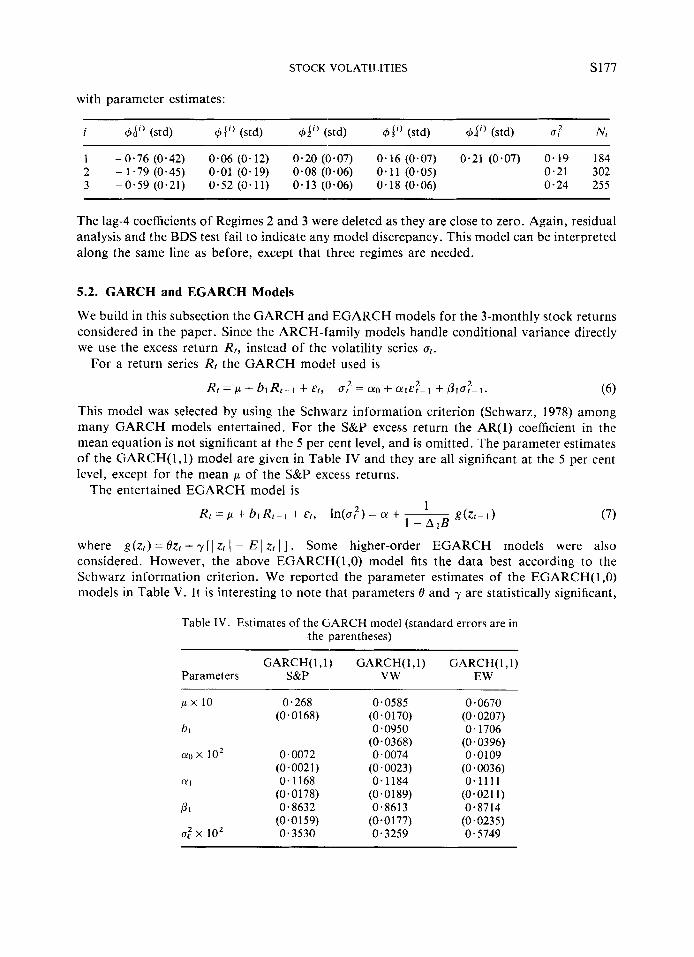
(6) This model was selected by using the Schwarz information criterion (Schwarz, 1978) among many GARCH models entertained. For the S&P excess return the AR(1) coefficient in the mean equation is not significant at the 5 per cent level, and is omitted. The parameter estimates of the GARCH(1,l) model are given in Table IV and they are all significant at the 5 per cent level, except for the mean p of the S&P excess returns.

2 2 Rr = p + bl Rt- 1 + ~ t , CT? = CYO + C Y I C ~ - I + P l ~ r - I .

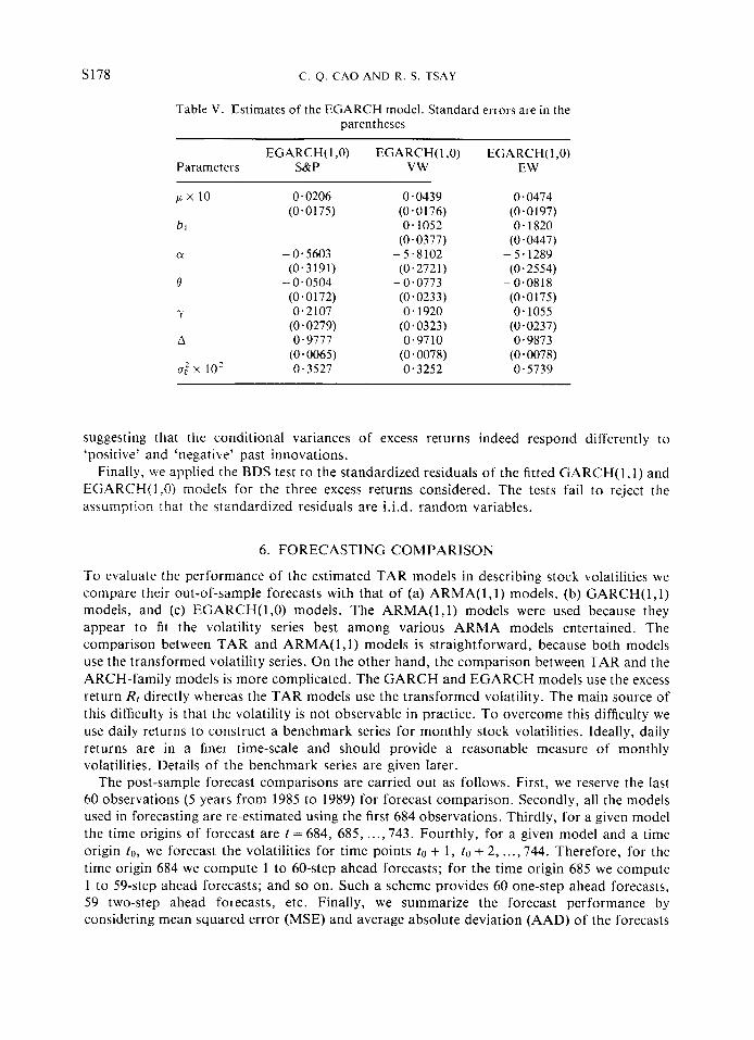
The entertained EGARCH model is 1

1 - A l B g(zr- 1 ) 2 Rr = p + b1 R r - I + E ( , ln(ur ) = a + ~ (7)

where g(z r ) = Bzr + y [ I zt I - E I zt 1 ] . Some higher-order EGARCH models were also considered. However, the above EGARCH(1,O) model fits the data best according to the Schwarz information criterion. We reported the parameter estimates of the EGARCH( 1,O) models in Table V. It is interesting to note that parameters 8 and y are statistically significant,

Table IV. Estimates of the GARCH model (standard errors are in the parentheses)

~~

GARCH(1,l) GARCH(1,l) GARCH(I,I) Parameters S&P VW EW

p x 10 0.268 0.0585 (0.0170) (0 * 0 168)

bi 0.0950 (0- 0368)

(Yo x lo2 0.0072 0.0074 (0.002 1) (0.0023)

011 0.1168 0.1184 (0.0 17 8) (0.01 89)

P I 0.8632 0.8613 (0.0 1 59) (0.01 77)

ff: x lo2 0.3530 0.3259

0.0670 (0 0207) 0.1706

(0.0396) 0.0109

(0.0036) 0.1111

0.8714 (0 -0235) 0.5749

(0.021 1)

S178 C. Q. CAO AND R. S. TSAY

Table V. Estimates of the EGARCH model. Standard errors are in the parentheses

EGARCH(1 ,O) EGARCH( I ,0) EGARCH( 1,O) Parameters S&P VW EW

p x 10 0.0206

bi (0.0175)

cy -0.5603 (0.3 191)

(0.0 172) -? 0.2107

(0.0279) A 0.9777

(0.0065) a: x 10’ 0.3527

8 - 0.0504

0-0439 (0.0176) 0.1052

(0.0377) -5‘8102 (0.272 1) - 0.0773 (0.0233) 0.1920

(0.0323) 0.9710

(0.0078) 0.3252

0.0474 (0.0 197) 0.1820

(0.0447) - 5.1289 (0.2554)

-0.0818 (0.0175) 0.1055

(0.0237) 0.9873

(0.0078) 0.5739

suggesting that the conditional variances of excess returns indeed respond differently to ‘positive’ and ‘negative’ past innovations.

Finally, we applied the BDS test to the standardized residuals of the fitted GARCH(1,l) and EGARCH(1,O) models for the three excess returns considered. The tests fail to reject the assumption that the standardized residuals are i.i.d. random variables.

6. FORECASTING COMPARISON

To evaluate the performance of the estimated TAR models in describing stock volatilities we compare their out-of-sample forecasts with that of (a) ARMA( 1 , l ) models, (b) GARCH(1,l) models, and (c) EGARCH(1,O) models. The ARMA(1,l) models were used because they appear to fit the volatility series best among various ARMA models entertained. The comparison between TAR and ARMA( 1, l ) models is straightforward, because both models use the transformed volatility series. On the other hand, the comparison between TAR and the ARCH-family models is more complicated. The GARCH and EGARCH models use the excess return RI directly whereas the TAR models use the transformed volatility. The main source of this difficulty is that the volatility is not observable in practice. To overcome this difficulty we use daily returns to construct a benchmark series for monthly stock volatilities. Ideally, daily returns are in a finer time-scale and should provide a reasonable measure of monthly volatilities. Details of the benchmark series are given later.

The post-sample forecast comparisons are carried out as follows. First, we reserve the last 60 observations (5 years from 1985 to 1989) for forecast comparison. Secondly, all the models used in forecasting are re-estimated using the first 684 observations. Thirdly, for a given model the time origins of forecast are t = 684, 685, ..., 743. Fourthly, for a given model and a time origin to, we forecast the volatilities for time points to + 1, to + 2, ..., 744. Therefore, for the time origin 684 we compute 1 to 60-step ahead forecasts; for the time origin 685 we compute 1 to 59-step ahead forecasts; and so on. Such a scheme provides 60 one-step ahead forecasts, 59 two-step ahead forecasts, etc. Finally, we summarize the forecast performance by considering mean squared error (MSE) and average absolute deviation (AAD) of the forecasts

STOCK VOLATlLITlES S179

by steps. Since fewer data points are available for longer-step ahead forecasts, we only report the comparison for 1 to 30-step.

6.1. Multi-step Ahead Forecasts

The multi-step ahead forecasts of TAR models are obtained by simulation. For a given TAR model for Y,, suppose that we want to forecast Y t + l , Yt+z, ..., Y r + h at the time origin f. We Grst use the model and the data, Y, for s < t , to generate 2000 realisations of { Y t + t ) := 1 . Then we average these realizations to obtain a mean series for time indices t + 1, ..., t + h and treat this mean series as our point forecasts. We ran some experiments with more than 2000 realizations and found that the forecasts are essentially the same.

6.2. TAR models versus ARMA models

Table VI shows the comparison between the ARMA and TAR models for the 3-monthly volatility series considered. It gives the MSE of TAR models for 1 to 30-step ahead forecasts

Table V1. Post-sample forecast comparison of MSE of TAR and ARMA models for the transformed volatility of monthly security excess returns, 1985-1989

S&P vw EW Lead time TAR ARMAITAR TAR ARM A/ T A R TAR ARMAITAR

1 0.161 1.065 0.214 1.021 0.281 0.907 2 0.168 1.028 0.21'7 1.004 0.261 0-963 3 0.159 1.046 0.204 1.019 0.216 0.979 4 0.161 1-060 0.204 1 *026 0.230 0.972 5 0.162 1-061 0.207 1.026 0.239 0.946 6 0.166 1.048 0.21 1 1 *029 0.242 0.949 7 0.162 1.052 0.201 1.028 0.234 0.969 8 0.159 1.036 0.201 0.992 0.225 0.956 9 0.158 1-046 0.198 1.009 0.228 0.969

10 0.163 1.009 0.204 0.979 0.232 0.958 I 1 0.167 1.025 0-208 0.993 0.240 0.952 12 0.166 1.067 0.20!> 1.026 0.250 0.963 13 0.171 1.039 0.215 1.010 0.252 0.950 14 0.166 1.067 0.21ti 1.014 0.245 0.960 15 0.165 1 *093 0.211; 1.031 0.250 0.955 16 0.168 1.089 0.219 1.033 0.254 0.947 17 0.175 I a088 0.230 1.018 0.265 0.955 18 0.172 1.113 0 * 22:' 1.048 0.268 0.967 19 0.175 I -086 0.198 1.028 0.271 0.943 20 0.172 1.102 0.194 1.042 0.272 0.941 21 0.174 1.093 0.197 1.027 0.278 0.939 22 0.169 1.069 0.191 1.018 0.283 0.930 23 0.173 1.051 0.195; 0.999 0.290 0.927 24 0.178 1.038 0.192: 1.000 0.291 0-930 25 0.180 1 *056 0.193 1.022 0 * 299 0.955 26 0-169 1-063 0.184- 1.026 0.302 0.939 27 0.177 1.023 0.190 0-995 0.310 0.931 28 0.183 1.027 0.194 1.007 0.315 0.959 29 0.187 1 -028 0.199 1.007 0.327 0.949 30 0.158 1.079 0-164 1-033 0.288 0.959

S180 C. Q. CAO AND R . S. TSAY

and the ratio of MSE of ARMA models to TAR models. From the table it is seen that the TAR models outperform the ARMA models for the S&P and value-weighted monthly excess returns, but the ARMA models are slightly more accurate than the TAR models in forecasting the volatility of monthly equal-weighted excess returns. The table also shows that in terms of mean squared error the difference between ARMA and TAR models is usually less than 10 per cent. Similar results hold for the AAD criterion.

6.3. Comparison Between Nonlinear Models

We now compare the performance of TAR models with that of the ARCH-family modeIs in (6) and (7). As mentioned above, the volatility of monthly excess returns for a stock is not observable, so that we construct a volatility series from the daily returns to serve as a benchmark series on which the forecasts can be compared. The constructed benchmark series for volatility consists of the monthly standard deviations computed from the daily portfolio returns. More specifically, consider the forecasting period from 1985 to 1989. Suppose that there are KI trading days in month t , then the monthly standard deviation of a daily stock return is

where denotes the ith trading day’s return in month t . This measure of monthly stock volatility was used before in French, Schwert, and Stambaugh (1987). Since the daily returns of the three stocks considered have significant lag-1 autocorrelation, the cross-product ri,trr+ I ,, is used in defining st.

The multi-step ahead forecasts of conditional variances for the GARCH(1,l) model in (6) were obtained by using an explicit functional form derived from the model in conjunction with the assumption that the error terms zr are i.i.d. N(0, 1). Details of the functional form is given in Appendix I. For the EGARCH(1,O) model in (7), we used the formula given in Appendix I1 to compute the forecasts of conditional variances. A square-root transformation is then taken to obtain monthly volatility forecasts. Finally, treating the data points of the benchmark series as observed monthly volatility, MSE and AAD of GARCH and EGARCH forecasts can be computed.

For the TAR models we modified the simulation procedure slightly in order to take care of the Box-Cox transformation used. The modification is that for each of the 2000 realizations of { Y t + / ) fz I we take the inverse transformation ut+/ = [( Yt+r/4) + 1 1 4 to obtain a realization of { u r + / ] . The mean series of these 2000 realizations of { @ f + h ) is then used to form the point forecasts of uf+h.

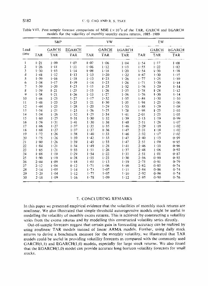
Tables VII and VIII report the results of 1 to 30-step ahead forecasts of TAR, GARCH(1,l) and EGARCH(1,O) models for the three monthly return series considered. The numbers shown in Table VII are the AAD of TAR models and the ratios of AAD between the ARCH-family models and the TAR models. From the table we observe that (a) the TAR models consistently have smaller AAD than the GARCH(1,l) and EGARCH(1,O) models for the monthly volatilities of S&P and value-weighted excess returns; (b) the gains of TAR models in both cases are more than 20 per cent for 8 to 25-step ahead forecasts; (c) for the equal-weighted excess returns the TAR model is slightly better at the short-term forecasts, but the EGARCH( 1,O) model is superior for the long-term forecasts.

The numbers shown in Table VIII are MSE of the TAR models and the ratios of MSE

STOCK VOLATILITIES S181

Table VII. Post-sample forecast comparison of AAD ( x lo2) of the TAR, GARCH and EGARCH models for the volatility of monthly security excess returns, 1985-1989

S&P vw EW

Lead GARCH EGARCH GARCH EGARCH GARCH EGARCH time TAR TAR TAR TAR TAR TAR TAR TAR TAR

.___

1 2 3 4 5 6 7 8 9

10 1 1 12 13 14 15 16 17 18 19 20 21 22 23 24 25 26 27 28 29 30

1.66 1.77 1.81 1.95 1.96 1 *97 1.98 1-98 1.91 1.98 1.96 1.99 1.99 2.04 2.05 2.10 2.10 2.06 2.08 2.14 2.18 2.16 2.19 2.20 2.19 2.31 2.41 2.44 2.42 2.47

1.09 1.04 1.10 1.06 1 . 1 5 1.12 1.17 1.13 1.19 1.17 1-18 1.17 1 *20 1 *20 1-20 1.22 1.25 1.28 1 *23 1.24 1.24 1.25 1.23 1.22 1 *26 1.26 1 *25 1.26 1.26 1.28 1.28 1.30 1 *30 1 *34 1-33 1.39 1.33 1.40 1.29 1.38 I .27 1.37 1.24 1.33 1.20 1-29 1.18 1.24 1-18 1.25 1.08 1.12 1 a01 1.03 1.01 1.04 1 *04 1 *05 1.03 1.03

1.76 1-80 1.80 1.94 1-96 1.96 1.96 1.96 1-90 1.94 1.93 1.96 1.96 1.99 2.03 2.05 2.08 2-03 2.05 2-10 2.14 2.15 2.16 2- 17 2-17 2-26 2.33 2-36 2-36 2-41

I .07 1 *03 1.11 1-09 1.18 1 . 1 5 1.18 1.14 1-20 1-19 1.19 1-18 1.21 1.19 1.21 1.22 1 *25 1.28 1-25 1.26 1.27 1.27 1-26 1-23 1 a27 1 *26 1 *27 1 *27 1.28 1.28 1.30 1.30 I *32 1.34 1.35 1-38 1.34 1.38 1.32 1.38 1.31 1.35 1.27 1.31 1 a24 I a26 1.23 1.22 1.21 1.20 1-13 1.10 1 *07 1-00 1-08 1 *oo 1.09 1.01 1-09 0.99

2-65 2.71 2.79 3.01 3-13 3.18 3.25 3.32 3.30 3.36 3.47 3.48 3.60 3.66 3.73 3.71 3.88 3-88 3.88 4.00 4.07 4.09 4.09 4.11 4.13 4.30 4.34 4.37 4.45 4.47

1.17 1.11 1-19 1-13 1.20 1.14

-16 1.10 -12 1-06 .11 1 *04 * l o 1-02 .07 1 *oo a 0 8 0-99 *08 0.98 .05 0-95 .06 0.94 .04 0.92 a03 0.91 a02 0.89 *04 0.90 *02 0.89

1-03 0.90 1.03 0.91 1 .oo 0.88 0-98 0.86 0.98 0.86 0.97 0.84 0.95 0.81 0.92 0.78 0.89 0.75 0.86 0.72 0.87 0.73 0.88 0.74 0-89 0-74

between the ARCH-family models and TAR models. By and large the results are similar to that of the AAD criterion. The TAR models outperform the ARCH-family models for S&P and value-weighted monthly excess returns. However, the EGARCH(1,O) model fares well in long horizon forecasts of monthly volatility of equal-weighted excess returns.

Since the S&P composite portfolio and the value-weighted composite portfolio represent large stocks and the equal-weighted portfolio represents small stocks, the results of forecasting comparison indicate that the TAR models might be useful in forecasting monthly volatility of large stocks. On the other hand the EGARCH(1,O) model can yield accurate long-term forecasts of monthly volatility for small stocks. We note that the above out-of-sample forecasts of the TAR model are unbiased, whereas those of the GARCH and EGARCH models are biased. The unfavourable performance of the ARCH-type models might be due in part to the forecasting bias.

S182 C. 0. CAO AND R. S. TSAY

Table VIII. Post-sample forecast comparison of MSE ( x l o3 ) of the TAR, GARCH and EGARCH models for the volatility of monthly security excess returns, 1985-1989

~~

S&P vw EW

Lead GARCH EGARCH GARCH EGARCH GARCH EGARCH time TAR TAR TAR

- TAR TAR TAR TAR TAR TAR

I 2 3 4 5 6 7 8 9

10 I 1 12 13 14 15 16 17 18 19 20 21 22 23 24 25 26 27 28 29 30

1.21 I .26 1.30 1.41 1.39 1.38 I .39 1.39 1.38 I .44 1.48 1.44 1.54 1.54 1.60 1.58 1.66 1.68 1.72 1.75 1.80 1.84 1 . 8 5 1-88 1.90 2.04 2 .12 2.14 2.20 2.18

1.09 I .07 1 . 1 1 1 . 1 1 1 .13 1.14 1.12 1.13 1.16 1.18 1.17 1.19 1.20 I .23 1.21 1.25 1.21 1.26 1.25 1.27 1.23 1.25 1.25 1.28 1.21 1.23 1.26 1.32 1.25 1.31 1.31 1.41 1.27 1.37 1.27 1-37 1.26 1-38 1.26 1.39 1.26 1-39 1.21 1.34 1.21 1.33 1.19 1.29 1.19 1.28 1.09 1-18 1.04 1.12 1.05 1.14 1.04 1.12 I .09 1.16

1 a07 1.06 1.08 1.13 1.13 1.14 1.15 1.15 1.13 1-17 1.21 1.20 1.26 1.25 1.30 1.30 1.35 1.37 I .40 I .42 1.45 1.49 1 . 5 1 I .54 1 . 5 5 1.65 1.71 1.73 1.77 1.78

1.06 I .04 1.12 1.13 1.18 1.20 1.20 1.22 1.23 I .26 1.23 1.26 1.25 1.32 I .26 1.33 1.27 1.36 1.32 1-35 1.30 1.35 1.29 1.33 1.25 1.28 1.34 1.41 1.32 1.39 1.38 1.48 1.35 1.46 1.36 1 .47 1.33 1.46 1.33 1.47 1-33 1.47 1.28 1.41 1 *26 1.37 1.22 1-31 1.23 1.30 1.13 1.19 1.06 1.10 1.07 1 . 1 1 I .07 1.10 I .09 1.12

1.54 1.55 1.54 I .67 1.77 1.71 1-76 1-78 1-76 1-84 1.94 1-88 I .98 2.01 2.13 2.11 2.29 2-31 2.32 2.40 2.51 2.46 2.48 2.51 2.56 2.75 2.82 2.84 2.92 2.85

1.17 1.08 1.22 1.12 1 .30 1.18 1.30 1.15 1.25 1.10 1.30 1.14 I .29 1.14 1.28 1.12 1.30 1.14 1-30 1.10 1.25 1 .06 1.29 I .08 1.23 I .02 1.25 1.05 1.19 0.99 1.26 1.07 1.18 1.02 1 .18 1.02 1.17 1.02 1.13 0.99 1.09 0.95 1.10 0.96 1.06 0.92 1.01 0.87 0.99 0.85 0.91 0.79 0.85 0.74 0.86 0.74 0.86 0.74 0.90 0.76

7. CONCLUDING REMARKS

In this paper we presented empirical evidence that the volatilities of monthly stock returns are nonlinear. We also illustrated that simple threshold autoregressive models might be useful in modelling the volatility of monthly excess returns. This is achieved by constructing a volatility series from the excess returns and by modelling this constructed volatility series directly.

Out-of-sample forecasts suggest that certain gain in forecasting accuracy can be realized by using nonlinear TAR models instead of linear ARMA models. Further, using daily stock returns to derive a benchmark measure for the monthly volatility, we illustrated that TAR models could be useful in providing volatility forecasts as compared with the commonly used GARCH( 1 , l ) and EGARCH( 1,O) models, especially for large stock returns. We also found that the EGARCH( 1,O) model can provide accurate long-horizon volatility forecasts for small stocks.

STOCK VOLATILITIES S183

APPENDIX I

In this appendix we present the formula used to calculate the multi-step ahead forecasts of the conditional variance for the GARCH( 1,l) model in (6). The variance equation of this model is a: = 010 + ale:- 1 + /3la:- 1. Denote the forecast origin by n and the forecast horizon by j . Let I, be the information set available at time n. For j = 1 the 1-step ahead forecast of the conditional variance is simply

E ( U i + l I I n ) = E(a0 + O1IE: + PlUfi I I n ) = 010 + ale; + /3,a;.

For j 2 2 , by using the assumption ihat Zr are i.i.d. N(0,l) and the identity E(r:+r I Z,) = E(af ,+/ I In), we have E(afi+j I I n ) = 010 + (011 + P l ) . E ( a i + j - ~ I I,). Therefore, the forecasts of conditional variances of a GARCH(1, 1) model can be computed recursively.

APPENDIX I1

Next we derive the formula for obtaining multi-step ahead forecasts of the conditional variance for the EGARCH model in (7). For simplicity we assume that the process is stationary SO that it starts with t = - co. The conditional variance of the model is

m 2 1

ln(at ) = a + ~ g(:lr-- I ) = 01 + Ak-lg(z,-k) 1 - A B k = 1

where g(z0 = 8zr + y [ I Zr I - E 1 zl I 1 . Therefore,

1 m

a f = e x p a + c Ak-'g(Zr-k) . [ k = l

Let n, j and I , be defined as in Appendix I . For j = 1 the 1-step ahead forecast of the conditional variance is simply

r m 1

For j = 2, the 2-step ahead forecast of the conditional variance is

r 1

m

a+ c Ak-'g(zn+z-k)] k = 2

where a(. ) is the cumulative distribution function of a standard normal variable. Similarly,

S184 C . Q. CAO AND R . S. TSAY

for j > 2, we have

x exp - (y- [ i:

ACKNOWLEDGEMENTS

This research is supported in par t by t h e Nat ional Science Foundat ion DMS-8902177 a n d DMS-9103250. T h e au thors wish to thank George C. T i a o f o r useful discussions, Kenneth R . French, Simon M. Pot te r , Daniel B. Nelson a n d t w o a n o n y m o u s referees f o r helpful comments and David Hsieh f o r providing t h e BDS-test p rogram.

REFERENCES

Bollerslev, T. (l986), ‘Generalized autoregressive conditional heterosccdasticity’, Journul of Econometrics, 31, 307-27.

Rollerslev, T., R. Y. Chou, and K. F. Kroner (1992), ‘ARCH modeling in finance: a review of the theory and empirical evidence’, Journal of Econometrics, 52, 5-60.

Brock, W . A., W. D. Dechert, and J . A. Scheinkman (1987), ‘A test for independence based on the correlation dimension’. Working paper, University of Wisconsin-Madison.

Engle, R. F. (1982), ‘Autoregressive conditional heteroscedasticity with estimates of the variance of U.K. inflation’, Econornetrica, 50, 987-1008.

French, K. R., G. W. Schwert, and R . Stambaugh (1987), ‘Expected stock returns and volatility’, Journal of Financial Economics, 19, 3-29.

Gallant, A. R., D. Hsieh, and G. E. Tauchen (1991), ‘On fitting a recalcitrant series: the pound/dollar exchange rate, 1974-83’, in W. Barnett, J . Powell, and G. Tauchen (eds), Nonpararnetric and Semiparametric Methods in Econometrics and Statistics, Cambridge University Press, Cambridge, pp.

Hsieh, D. (1989), ‘Testing for nonlinear dependence in daily foreign exchange rates’, Journal of

Hsieh, D., and B. LeBaron (1988), ‘Small sample properties of the BDS statistics, I , I1 and 111’. Working

LeBaron, B. (1992), ‘Some relations between volatility and serial correlations in stock market returns’,

Luukkonen, R., P. Saikkonen, and T. Terasvirta, (1988), ‘Testing linearity against smooth transition

Melino, A., and S. M. Turnbull (1990), ‘Pricing foreign currency options with stochastic volatility’,

Nelson, D. B., and C. Q. Cao (1992), ‘Inequality constraints in the univariate GARCH model’, Journal

Nelson, D. B. (1991), ‘Conditional heteroscedasticity in asset returns: a new approach’, Econornetrica,

Pagan A., and G. W . Schwert (1990), ‘Alternative models for conditional stock volatility’, Joitrnal of

199-240.

Business, 62, 339-368.

paper, University of Chicago and University of Wisconsin-Madison.

Journal of Business, 65, 199-220.

autoregressive models’, Biometrika, 75, 491-499.

Journal of Econometrics, 45, 239-266.

of Business & Economic Statistics, 10, 229-235.

59, 347-370.

Econometrics, 45, 267-290.

STOCK VOL AT I I . IT I ES S185

Poterba. J . , and L. Summers (1986), ‘The persistence of volatility and stock market fluctuations’,

Quandt, R . E., and J . Ramsey. (1978), ‘Estimating mixtures of normal distributions and switching

Schwarz, G. (1978), ‘Estimating the dimension of a model’, Annual of Statistics, 6, 461-464. Scheinkman, J . A. , and B. LeBaron (19891, ‘Nonlinear dynamics and stock returns’, Joztrnal of

Schwert, G . W. (1990), ‘Stock volatility and the crash of ‘87’, Review ofFinancial Studies, 3, 77-102. Schwert, G. W., and P. J . Seguin (1990), ‘Hetemscedasticity in stock returns’, Journal of Finance, 4,

Scott, L. 0. (1987), ‘Option pricing when the variance changes randomly: theory, estimation and an

Stein, J . (1989), ‘Overreaction in the option market’, Journal of Finance, 44, 1011-1023. Taylor, S. (1986), Modeling Finuncial Time Serim, John Wiley & Sons, Chichester. Tong, H. (1990). Nonlinear Time Series: A Djnamical System Approach, Oxford University Press,

Tsay, R . S. (1986), ‘Nonlinearity tests for time series’, Bionietrika, 73, 461-466. Tsay, R. S. (1987), ‘Conditional heteroscedastic time series models’, Journal of the Arnerican Statistical

Tsay, R . S . (1989), ‘Testing and modeling threshold autoregressive processes’, Journal of the A~nerican

Tsay, R . S. (l991), ‘Modelling nonlinearity in univariate time series analysis’, Statisrical Sinica, I ,

Wiggins, J . B. (1987), ‘Option values under stochastic volatility: theory and empirical estimations’,

American Economic Review, 76, 1 142- 1 15 1.

t-egressions’, Joitrnal of the American Statistical Association, 13, 730-138.

Business, 3, 311-337.

1129- 1 155.

application’, Journal of Financial and Quanti,’ative Analysis, 22, 419-438.

London.

Association, 82, 590-604.

Statistical Association, 84, 23 1-240.

43 1-452.

Joirrnal of Financial Econornics, 19, 35 1-372.