Nonlinear Programming

3rd Edition

Theoretical Solutions Manual

Chapter 6

Dimitri P. Bertsekas

Massachusetts Institute of Technology

Athena Scientific, Belmont, Massachusetts

1

NOTE

This manual contains solutions of the theoretical problems, marked in the book by It is

continuously updated and improved, and it is posted on the internet at the book’s www page

http://www.athenasc.com/nonlinbook.html

Many thanks are due to several people who have contributed solutions, and particularly to David

Brown, Angelia Nedic, Asuman Ozdaglar, Cynara Wu.

Last Updated: May 2016

2

Section 6.1

Solutions Chapter 6

SECTION 6.1

6.1.4

Throughout this exercise we will use the fact that strong duality holds for convex quadratic

problems with linear constraints (cf. Section 4.4).

The problem of finding the minimum distance from the origin to a line is written as

min1

2‖x‖2

subject to Ax = b

where A is a 2× 3 matrix with full rank, and b ∈ <2. Let f∗ be the optimal value and consider

the dual function

q(λ) = minx

{1

2‖x‖2 + λ′(Ax− b)

}.

Let V ∗ be the supremum over all distances of the origin from planes that contain the line

{x | Ax = b}. Clearly, we have V ∗ ≤ f∗, since the distance to the line {x | Ax = b} cannot be

smaller that the distance to the plane that contains the line.

We now note that any plane of the form {x | p′Ax = p′b}, where p ∈ <2, contains the line

{x | Ax = b}, so we have for all p ∈ <2,

V (p) ≡ minp′Ax=p′x

1

2‖x‖2 ≤ V ∗.

On the other hand, by duality in the minimization of the preceding equation, we have

U(p, γ) ≡ minx

{1

2‖x‖2 + γ(p′Ax− p′x)

}≤ V (p), ∀ p ∈ <2, γ ∈ <.

Combining the preceding relations, it follows that

supλq(λ) = sup

p,γU(p, γ) ≤ sup

pU(p, 1) ≤ sup

pV (p) ≤ V ∗ ≤ f∗.

Since by duality in the original problem, we have supλ q(λ) = f∗, it follows that equality holds

throughout above. Hence V ∗ = f∗, which was to be proved.

3

Section 6.1

6.1.7 (Duality Gap of the Knapsack Problem)

(a) Let

xi =

{1 if the ith object is included in the subset,

0 otherwise.

Then the total weight and value of objects included is∑i wixi and

∑i vixi, respectively, and the

problem can be written as

maximize f(x) =

n∑i=1

vixi

subject to

n∑i=1

wixi ≤ A, xi ∈ {0, 1}, i = 1, . . . , n.

(b) Let f(x) = −f(x) and consider the equivalent problem of minimizing f(x) subject to the

constraints given above. Then

L(x, µ) = −n∑i=1

vixi + µ

(n∑i=1

wixi −A

),

and

q(µ) = infxi∈{0,1}

{n∑i=1

(µwi − vi)xi − µA

}.

Note that the minimization above is a separable problem, and the infimum is attained at

xi(µ) =

0 if µ > vi/wi,

1 if µ < vi/wi,

0 or 1 if µ = vi/wi.

Without loss of generality, assume that the objects are ordered such that v1w1≤ v2

w2≤ . . . ≤ vn

wn.

When µ ∈(vj−1

wj−1,vjwj

]for some j with 1 ≤ j ≤ n, then xi(µ) = 1 for all i ≥ j and xi(µ) = 0

otherwise, and

q(µ) = µ

n∑i=j

wi −A

− n∑i=j

vi.

From this relation, we see that, as µ increases, the slope of q(µ) decreases from∑ni=1 wi − A to

−A. Therefore, if∑ni=1 wi − A > 0, q(µ) is maximized when the slope of the curve goes from

positive to negative. In this case, the dual optimal value q∗ is attained at µ∗ =vi∗wi∗

, where i∗ is

the largest i such that

wi + . . .+ wn ≥ A.

If∑ni=1 wi −A ≤ 0, then the dual optimal value q∗ is attained at µ∗ = 0.

4

Section 6.1

(c) Consider a relaxed version of the problem of minimizing f :

minimize fR(x) = −n∑i=1

vixi

subject to

n∑i=1

wixi ≤ A, xi ∈ [0, 1], i = 1, . . . , n.

Let f∗R and q∗R be the optimal values of the relaxed problem and its dual, respectively. In the

relaxed problem, the cost function is convex over <n (in fact it is linear), and the constraint set

is polyhedral. Thus, according to Prop. 6.2.1, there is no duality gap, and f∗R = q∗R. The dual

function of the relaxed problem is

qR(µ) = infxi∈[0,1]

{n∑i=1

(µwi − vi)xi − µA+

}.

Again, qR(µ) is separable and the infimum is attained at

xi(µ) =

0 if µ > vi/wi,

1 if µ < vi/wi,

anything in [0, 1] if µ = vi/wi.

Thus the solution is the same as the {0, 1} constrained problem for all i with µ 6= vi/wi. For i

with µ = vi/wi, the value of xi is irrelevant to the dual function value. Therefore, q(µ) = qR(µ)

for all µ, and thus q∗ = q∗R.

Following Example 6.1.2, it can be seen that the optimal primal and dual solution pair

(x∗, µ∗) of the relaxed problem satisfies

µ∗wi = vi, if 0 < x∗i < 1,

µ∗wi ≥ vi, if x∗i = 0,

µ∗wi ≤ vi, if x∗i = 1.

In fact, it is straightforward to show that there is an optimal solution of the relaxed problem

such that at most one x∗i satisfies 0 < x∗i < 1. Consider a solution x equivalent to this optimal

solution with the exception that xi = 0 if 0 < x∗i < 1. This solution is clearly feasible for the

{0, 1} constrained problem, so that we have

f∗ ≤ f(x) ≤ f∗R + max1≤i≤n

vi.

Combining with earlier results,

f∗ ≤ q∗R + max1≤i≤n

vi = q∗ + max1≤i≤n

vi.

5

Section 6.1

Since f∗ = −f∗ and q∗ = −q∗, we have the desired result.

(d) Since the object weights and values remain the same we have from (c) that 0 ≤ q∗(k)−f∗(k) ≤

max1≤i≤n vi. By including in the subset each replica of an object assembled in the optimal

solution to the original problem, we see that f∗(k) ≥ kf∗. It then follows that

limk→∞

q∗(k)− f∗(k)

f∗(k)= 0.

6.1.8 (Sensitivity)

We have

f = infx∈X

{f(x) + µ′

(g(x)− u

)},

f = infx∈X

{f(x) + µ′

(g(x)− u

)},

from which

f − f = infx∈X

{f(x) + µ′

(g(x)− u

)}− infx∈X

{f(x) + µ′

(g(x)− u

)}+ µ′(u− u)

≥ µ′(u− u),

where the last inequality holds because µ is a dual-optimal solution of the problem

minimize f(x)

subject to x ∈ X, g(x) ≤ u,

so that it maximizes over µ ≥ 0 the dual value infx∈X{f(x) + µ′

(g(x)− u

)}.

This proves the left-hand side of the desired inequality. Interchanging the roles of f , u, µ,

and f , u, µ, shows the desired right-hand side.

6.1.9 (Hoffman’s Bound)

(a) Since the feasible set is closed, the projection problem given in the exercise has an optimal

solution. Therefore by Proposition 3.4.2, there exists an optimal primal solution and geometric

multiplier pair (x∗(y, z), µ∗(y, z)) for each y ∈ Y, z ∈ <n. By the optimality condition, for µ to

be a geometric multiplier, it suffices that

− z − x∗‖z − x∗‖

=∑

i∈I(x∗(y,z)

µiai,

where I(x∗(y, z)) is the set of indexes corresponding to the active constraints at x∗(y, z), and ai

is the ith column vector of A′. Since the vector in the left-hand-side of the equation has norm

6

Section 6.1

1, we can pick µ∗(y, z) to be the minimum norm solution for this linear equation. Since there

are only a finite number of such equations, the set {µ∗(y) | y ∈ Y } is bounded. Finally, by the

optimality of a geometric multiplier, we have

f∗(y, z) ≤ ‖z − z‖+ µ∗(y, z)′(Az − b− y) ≤ µ∗(y, z)′(Az − b− y)+.

(b) Using the last inequality in part (a), we have

f∗(y, z) ≤∑i

µ∗i (y, z)‖(Az − b− y)+‖, ∀y ∈ Y, z ∈ Z,

and

f∗(y, z) ≤ maxiµ∗i (y, z) ‖(Az − b− y)+‖, ∀y ∈ Y, z ∈ <n.

Let c be a constant such that c > {µ∗(y) | y ∈ Y }. By the boundedness of {µ∗(y) | y ∈ Y } shown

in part (a), we can choose c so that the bound f∗(y, z) ≤ c‖(Ax− b− y)+‖ holds.

6.1.10 (Upper Bounds to the Optimal Dual Value [Ber99])

We consider the subset of <r+1

A ={

(z, w) | there exists x ∈ X such that g(x) ≤ z, f(x) ≤ w},

and its convex hull Conv(A). The vectors(g(xF ), f(xF )

)and

(g(xI), f(xI)

)belong to A. In

addition, the vector (0, f), where

f = inf{w | (z, w) ∈ Conv(A), z ≤ 0

},

is in the closure of Conv(A). Let us now show that q∗ ≤ f , as indicated by Fig. 1.

Indeed, for each (z, w) ∈ Conv(A), there exist ξ1 ≥ 0 and ξ2 ≥ 0 with ξ1 + ξ2 = 1, and

x1 ∈ X, x2 ∈ X such that

ξ1g(x1) + ξ2g(x2) ≤ z,

ξ1f(x1) + ξ2f(x2) ≤ w.

Furthermore, by the definition of the dual function q, we have for all µ ∈ <r,

q(µ) ≤ f(x1) + µ′g(x1),

q(µ) ≤ f(x2) + µ′g(x2).

7

Section 6.1

Combining the preceding four inequalities, we obtain

q(µ) ≤ w + µ′z, ∀ (z, w) ∈ Conv(A), µ ≥ 0.

The above inequality holds also for all (z, w) that are in the closure of Conv(A), and in particular,

for (z, w) = (0, f). It follows that

q(µ) ≤ f , ∀ µ ≥ 0,

from which, by taking the maximum over µ ≥ 0, we obtain q∗ ≤ f .

Let γ be any nonnegative scalar such that g(xI) ≤ −γg(xF ), and consider the vector

∆ = −γg(xF )− g(xI).

Since ∆ ≥ 0, it follows that the vector

(−γg(xF ), f(xI)

)=(g(xI) + ∆, f(xI)

)also belongs to the set A. Thus the three vectors

(g(xF ), f(xF )

), (0, f),

(−γg(xF ), f(xI)

)belong to the closure of Conv(A), and form a triangle in the plane spanned by the “vertical”

vector (0, 1) and the “horizontal” vector(g(xF ), 0

).

Let (0, f) be the intersection of the vertical axis with the line segment connecting the vectors(g(xF ), f(xF )

)and

(−γg(xF ), f(xI)

)(there is a point of intersection because γ ≥ 0). We have

by Euclidean triangle geometry (cf. Fig. 1)

f − f(xI)

f(xF )− f(xI)=

γ

γ + 1. (1)

Since the vectors(g(xF ), f(xF )

)and

(−γg(xF ), f(xI)

)both belong to Conv(A), we also have

(0, f) ∈ Conv(A). By the definition of f , we obtain f ≤ f , and since q∗ ≤ f , as shown earlier,

from Eq. (1) we have

q∗ − f(xI)

f(xF )− f(xI)≤ f − f(xI)

f(xF )− f(xI)≤ γ

γ + 1.

Taking the infimum over γ ≥ 0, the desired error bound follows.

8

Section 6.1

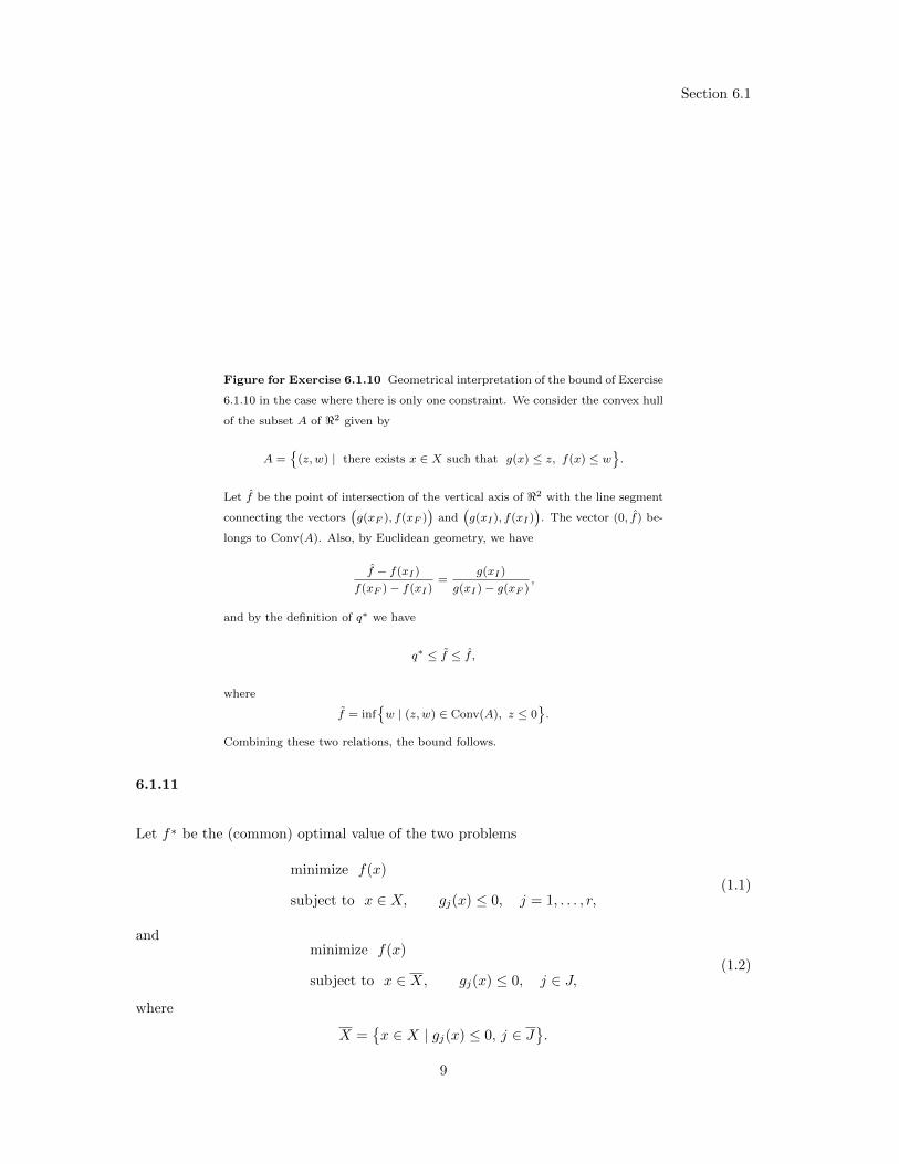
Figure for Exercise 6.1.10 Geometrical interpretation of the bound of Exercise

6.1.10 in the case where there is only one constraint. We consider the convex hull

of the subset A of <2 given by

A ={

(z, w) | there exists x ∈ X such that g(x) ≤ z, f(x) ≤ w}.

Let f be the point of intersection of the vertical axis of <2 with the line segment

connecting the vectors(g(xF ), f(xF )

)and

(g(xI), f(xI)

). The vector (0, f) be-

longs to Conv(A). Also, by Euclidean geometry, we have

f − f(xI)

f(xF )− f(xI)=

g(xI)

g(xI)− g(xF ),

and by the definition of q∗ we have

q∗ ≤ f ≤ f ,

where

f = inf{w | (z, w) ∈ Conv(A), z ≤ 0

}.

Combining these two relations, the bound follows.

6.1.11

Let f∗ be the (common) optimal value of the two problems

minimize f(x)

subject to x ∈ X, gj(x) ≤ 0, j = 1, . . . , r,(1.1)

andminimize f(x)

subject to x ∈ X, gj(x) ≤ 0, j ∈ J,(1.2)

where

X ={x ∈ X | gj(x) ≤ 0, j ∈ J

}.

9

Section 6.1

Since {µ∗j | j ∈ J} is a geometric multiplier of problem (1.2), we have

f∗ = infx∈X

f(x) +∑j∈J

µ∗jgj(x)

. (1.3)

Since the problem

minimize

f(x) +∑j∈J

µ∗jgj(x)

subject to x ∈ X, gj(x) ≤ 0, j ∈ J,

(1.4)

has no duality gap, we have

infx∈X

f(x) +∑j∈J

µ∗jgj(x)

= supµj≥0, j∈J

infx∈X

f(x) +∑j∈J

µ∗jgj(x) +∑j∈J

µjgj(x)

. (1.5)

Combining Eqs. (1.3) and (1.5), we have

f∗ = supµj≥0, j∈J

infx∈X

f(x) +∑j∈J

µ∗jgj(x) +∑j∈J

µjgj(x)

,

which can be written as

f∗ = supµj≥0, j∈J

q({µ∗j | j ∈ J}, {µj | j ∈ J}

),

where q is the dual function of problem (1.1). It follows that problem (1.1) has no duality gap.

If {µ∗j | j ∈ J} is a geometric multiplier for problem (1.4), we have

infx∈X

f(x) +∑j∈J

µ∗jgj(x)

= infx∈X

f(x) +∑j∈J

µ∗jgj(x) +∑j∈J

µ∗jgj(x)

,

which together with Eq. (1.3), implies that

f∗ = infx∈X

f(x) +∑j∈J

µ∗jgj(x) +∑j∈J

µ∗jgj(x)

,

or that {µ∗j | j = 1, . . . , r} is a geometric multiplier for the original problem (1.1).

6.1.12 (Extended Representation)

(a) Consider the problems

minimize f(x)

subject to x ∈ X, gj(x) ≤ 0, j = 1, . . . , r,(1.6)

10

Section 6.1

and

minimize f(x)

subject to x ∈ X, gj(x) ≤ 0, j = 1, . . . , r, gj(x) ≤ 0, j = 1, . . . , r,(1.7)

where

X = X ∩{x | gj(x) ≤ 0, j = 1, . . . , r

},

and let f∗ be their (common) optimal value.

If problem (1.7) has no duality gap, we have

f∗ = supµ≥0, µ≥0

infx∈X

f(x) +

r∑j=1

µjgj(x) +

r∑j=1

µj gj(x)

≤ supµ≥0, µ≥0

infx∈X

gj(x)≤0, j=1,...,r

f(x) +

r∑j=1

µjgj(x) +

r∑j=1

µj gj(x)

= supµ≥0, µ≥0

infx∈X

f(x) +

r∑j=1

µjgj(x) +

r∑j=1

µj gj(x)

≤ supµ≥0, µ≥0

infx∈X

f(x) +

r∑j=1

µjgj(x)

= supµ≥0

infx∈X

f(x) +

r∑j=1

µjgj(x)

= supµ≥0

q(µ),

where q is the dual function of problem (1.6). Therefore, problem (1.6) has no duality gap.

(b) If µ∗ = {µ∗j | j = 1, . . . , r}, and µ∗ = {µ∗j | j = 1, . . . , r}, are geometric multipliers for

problem (1.7), we have

f∗ = infx∈X

f(x) +r∑j=1

µ∗jgj(x) +r∑j=1

µ∗j gj(x)

≤ inf

x∈Xgj(x)≤0, j=1,...,r

f(x) +

r∑j=1

µ∗jgj(x) +

r∑j=1

µ∗j gj(x)

= infx∈X

f(x) +

r∑j=1

µ∗jgj(x) +

r∑j=1

µ∗j gj(x)

≤ infx∈X

f(x) +

r∑j=1

µ∗jgj(x)

= infx∈X

f(x) +

r∑j=1

µ∗jgj(x)

= q(µ∗).

11

Section 6.2

It follows that µ∗ is a geometric multiplier for problem (1.6).

SECTION 6.2

6.2.2 (A Stronger Version of the Duality Theorem)

Without loss of generality, we may assume that there are no equality constraints, so that the

problem isminimize f(x)

subject to x ∈ X, a′jx− bj ≤ 0, j = 1, . . . , r.

Let X = C ∩ P , and let the polyhedron P be described in terms of linear inequalities as

P = {x ∈ <n | a′jx− bj ≤ 0, j = r + 1, . . . , p},

where p is an integer with p > r. By applying Lemma 6.2.2 with

S = {x ∈ <n | a′jx− bj ≤ 0, j = 1, . . . , p},

and F (x) = f(x)− f∗, we have that there exist scalars µi ≥ 0, j = 1, . . . , p, such that

f∗ ≤ f(x) +

p∑j=1

µj(a′jx− bj), ∀ x ∈ C.

For any x ∈ X we have µj(a′jx − bj) ≤ 0 for all j = r + 1, . . . , p, so the above relation implies

that

f∗ ≤ f(x) +

r∑j=1

µj(a′jx− bj), ∀ x ∈ X,

or equivalently

f∗ ≤ infx∈X{f(x) +

r∑j=1

µj(a′jx− bj)} = q(µ) ≤ q∗.

By using the weak duality theorem (Prop. 6.1.3), it follows that µ is a Lagrange multiplier and

that there is no duality gap.

In Example 6.2.1, we can set C = {x ∈ <2 | x ≥ 0} and P = {x ∈ <2 | x1 ≥ 0}. Then

evidently X = C and f is convex over C. However, ri(C) = int(C) = {x ∈ <2 | x > 0}, while

every feasible point x must have x1 = 0. Hence no feasible point belongs to the relative interior

of C, and as seen in Example 6.2.1, there is a duality gap.

12

Section 6.3

SECTION 6.3

6.3.1 (Boundedness of the Set of Geometric Multipliers)

Assume that there exists an x ∈ X such that gj(x) < 0 for all j. By Prop. 6.3.1, the set of

Lagrange multipliers is nonempty. Let µ be any Lagrange multiplier. By assumption, −∞ < f∗,

and we have

−∞ < f∗ ≤ L(x, µ) = f(x) +

r∑j=1

µjgj(x),

or

−r∑j=1

µjgj(x) ≤ f(x)− f∗.

We have

mini=1,...,r

{−gi(x)} ≤ −gj(x), ∀ j,

so by combining the last two relations, we obtain r∑j=1

µj

mini=1,...,r

{−gi(x)} ≤ f(x)− f∗.

Since x satisfies gj(x) < 0 for all j, we have

r∑j=1

µj ≤f(x)− f∗

minj=1,...,r{−gj(x)}.

Hence the set of Lagrange multipliers is bounded.

Conversely, let the set of Lagrange multipliers be nonempty and bounded. Consider the set

B ={z | there exists x ∈ X such that g(x) ≤ z

}.

Assume, to arrive at a contradiction, that there is no x ∈ X such that g(x) < 0. Then the origin

is not an interior point of B, and similar to the proof of Prop. 6.3.1, we can show that B is

convex, and that there exists a hyperplane whose normal γ satisfies γ 6= 0, γ ≥ 0, and

γ′g(x) ≥ 0, ∀ x ∈ X. (1)

Let now µ be a Lagrange multiplier. Using Eq. (1), we have for all β ≥ 0

f∗ = infx∈X

L(x, µ) ≤ infx∈X

L(x, µ+ βγ) ≤ infx∈X, g(x)≤0

L(x, µ+ βγ) ≤ infx∈X, g(x)≤0

f(x) = f∗,

where the last inequality holds because µ + βγ ≥ 0, and hence (µ + βγ)′g(x) ≤ 0 if g(x) ≤ 0.

Hence, equality holds throughout in the above relation, so µ+βγ is a Lagrange multiplier for all

β ≥ 0. Since γ 6= 0, it follows that the set of Lagrange multipliers is unbounded – a contradiction.

13

Section 6.3

6.3.2 (Optimality Conditions for Nonconvex Cost)

(a) Since the constraint set X = {x | x ∈ X, gj(x) ≤ 0, j = 1, . . . , r} is convex, and x∗ is a local

minimum, we have

∇f(x∗)′(x− x∗) ≥ 0, ∀ x ∈ X

(see Prop. 2.1.2 of Chapter 2). Hence x∗ is a local minimum of the problem

minimize ∇f(x∗)′x

subject to x ∈ X, gj(x) ≤ 0, j = 1, . . . , r.(1)

he Assumption 6.3.1 holds for problem (1), so that we can apply Prop. 6.3.1. Thus we have that

there is no duality gap, and there exists a Lagrange multiplier µ∗ ≥ 0 for problem (1), i.e.

supµ≥0

q(µ) = q(µ∗) = infx∈X

∇f(x∗)′x+

r∑j=1

µ∗jgj(x)

= ∇f(x∗)′x∗.

From Prop. 6.1.1, we also obtain

µ∗jgj(x∗) = 0, ∀ j.

The last two relations imply that

x∗ ∈ arg minx∈X

∇f(x∗)′x+

r∑j=1

µ∗jgj(x)

. (2)

(b) We use Prop. 4.3.12 to assert that there exist µ∗j ≥ 0, j = 1, . . . , r, such that µ∗jgj(x∗) = 0

for all j and

∇xL(x∗, µ∗)′(x− x∗) ≥ 0, ∀ x ∈ X.

The last relation implies that

x∗ = arg minx∈X∇xL(x∗, µ∗)′x.

6.3.3 (Boundedness of the Set of Lagrange Multipliers for Nonconvex

Constraints)

For simplicity and without loss of generality, assume that A(x∗) = {1, . . . , r}, and denote

hj(x) = ∇gj(x∗)′(x− x∗), ∀ j.

14

Section 6.3

By Prop. 6.1.1, µ ∈M∗ if and only if x∗ is a global minimum of the convex problem

minimize ∇f(x∗)′(x− x∗)

subject to x ∈ X, hj(x) ≤ 0, j = 1, . . . , r,(1)

while µ is a Lagrange multiplier. The feasible directions of X at x∗ are the vectors of the form

d = x− x∗ where x ∈ X. Hence the assumption that there exists a feasible direction d with the

property described is equivalent to the existence of an x ∈ X such that hj(x) < 0 for all j.

If there exists a feasible direction d with ∇gj(x∗)′d < 0 for all j, then by Prop. 4.3.12, the

set M∗ is nonempty. Applying the result of Exercise 6.3.1 to problem (1), we see that the set M∗

is bounded. Conversely, if M∗ is nonempty and bounded, again applying the result of Exercise

6.3.1, we see that there exists x ∈ X such that hj(x) < 0 for all j, and hence also there exists a

feasible direction with the required property.

6.3.4 (Characterization of Pareto Optimality)

(a) Assume that x∗ is not a Pareto optimal solution. Then there is a vector x ∈ X such that

either

f1(x) ≤ f1(x∗), f2(x) < f2(x∗),

or

f1(x) < f1(x∗), f2(x) ≤ f2(x∗).

In either case, by using the facts λ∗1 > 0 and λ∗2 > 0, we have

λ∗1f1(x) + λ∗2f2(x) < λ∗1f1(x∗) + λ∗2f2(x∗),

yielding a contradiction. Therefore x∗ is a Pareto optimal solution.

(b) Let

A = {(z1, z2) | there exists x ∈ X such that f1(x) ≤ z1, f2(x) ≤ z2}.

We first show that A is convex. Indeed, let (a1, a2), (b1, b2) be elements of A, and let (c1, c2) =

α(a1, a2)+(1−α)(b1, b2), for any α ∈ [0, 1]. Then for some xa ∈ X, xb ∈ X, we have f1(xa) ≤ a1,

f2(xa) ≤ a2, f1(xb) ≤ b1, and f2(xb) ≤ b2. Let xc = αxa + (1−α)xb. Since X is convex, xc ∈ X,

and since f1 and f2 are convex, we have

f1(xc) ≤ c1, f2(xc) ≤ c2.

Hence (c1, c2) ∈ A implying that A is convex.

15

Section 6.3

Note that(f1(x∗), f2(x∗)

)is not an interior point of A. [If this were not the case, then for

some x ∈ X we would have f1(x) < f1(x∗) and f2(x) < f2(x∗), so that x∗ would not be Pareto

optimal.] By supporting hyperplane theorem, there exist λ∗1 and λ∗2, not both equal to 0, such

that

λ∗1z1 + λ∗2z2 ≥ λ∗1f1(x∗) + λ∗2f2(x∗), ∀ (z1, z2) ∈ A.

Since z1 and z2 can be arbitrarily large, we must have λ∗1 ≥ 0 and λ∗2 ≥ 0. Furthermore, by the

definition of the set A, from the above equation we obtain

λ∗1f1(x) + λ∗2f2(x) ≥ λ∗1f1(x∗) + λ∗2f2(x∗), ∀ x ∈ X,

implying that

minx∈X

{λ∗1f1(x) + λ∗2f2(x)

}= λ∗1f1(x∗) + λ∗2f2(x∗).

(c) Generalization of (a): If x∗ is a vector in X, and λ∗1, . . . , λ∗m are positive scalars such that

m∑i=1

λ∗i fi(x∗) = min

x∈X

{m∑i=1

λ∗i fi(x)

},

then x∗ is a Pareto optimal solution.

Generalization of (b): Assume that X is convex and f1, . . . , fm are convex over X. If x∗ is a

Pareto optimal solution, then there exist non-negative scalars λ∗1, . . . , λ∗m, not all zero, such that

m∑i=1

λ∗i fi(x∗) = min

x∈X

{m∑i=1

λ∗i fi(x)

}.

6.3.5 (Directional Convexity)

LetA = {(z, w) | there exists (x, u) ∈ <n+s such that

h(x, u) = z, f(x, u) ≤ w, u ∈ U}.

Suppose that (0, f∗) is an interior point of A. Then the point (0, f∗ − δ) belongs to A for some

small enough δ > 0. By definition of the set A, we have that h(x, u) = 0 and f(x, u) ≤ f∗ − δ

for some x ∈ <n and u ∈ U , which contradicts the fact that f∗ is the optimal value. Therefore

(0, f∗) must be on the boundary of the set A. Furthermore, there is a supporting hyperplane of

the set A that passes through the point (0, f∗). In other words, there exists a nonzero vector

(λ, β) such that

βf∗ ≤ λ′z + βw, ∀(z, w) ∈ A. (1)

16

Section 6.3

By assumption (2), we have that for z = 0 there are a vector u ∈ U and a vector x ∈ <n

such that h(x, u) = 0, which implies that (0, w) ∈ A for all w with w ≥ f(x, u) ≥ f∗. Then from

(1) we have

0 ≤ β(w − f∗), ∀ w ≥ f∗,

which holds only if β ≥ 0. Suppose that β = 0. Then assumption (2) and Eq. (1) imply that

λ′z ≥ 0, ∀ z with ||z|| < ε,

which is possible only if λ = 0. But this contradicts the fact that (λ, β) 6= 0. Hence, we can take

β = 1 in Eq. (1). From here and the definition of the set A, we obtain

f∗ ≤ f(x, u) + λ′h(x, u), ∀ x ∈ <n, u ∈ U.

This, combined with weak duality, implies that

infx∈<n,u∈U

{f(x, u) + λ′h(x, u)

}= f∗. (2)

Suppose that (x∗, u∗) is an optimal solution. Then (x∗, u∗) must be feasible [i.e., it must

satisfy h(x∗, u∗) = 0], and

f∗ = f(x∗, u∗) + λ′h(x∗, u∗) = infx∈<n,u∈U

{f(x, u) + λ′h(x, u)} ,

where the last equality follows from Eq. (2). Therefore we must have

u∗ = arg minu∈U{f(x∗, u) + λ′h(x∗, u)} .

Similarly, we can argue that

x∗ = arg minx∈<n

{f(x, u∗) + λ′h(x, u∗)} .

If f and h are continuously differentiable with respect to x for any u ∈ U , the last relation implies

that

∇xf(x∗, u∗) +∇xh(x∗, u∗)λ = 0.

17

Section 6.3

6.3.6 (Directional Convexity and Optimal Control)

Similar to Exercise 6.3.5, we can show that there is a vector (−p∗, 1) such that

f∗ ≤ −p∗′z + w, ∀ (z, w) ∈ A,

where p∗ ∈ <N . This implies

f∗ ≤ infxi∈<,i=1,...,N

infui∈Ui,i=0,...,N−1

{N−1∑i=0

(p∗i+1

′fi(xi, ui) + gi(xi, ui)− p∗i+1′xi+1

)+ gN (xN )

}

= infxi∈<, i=1,...,N

{gN (xN ) +

N−1∑i=0

(infui∈Ui

{p∗i+1

′fi(xi, ui) + gi(xi, ui)}− p∗i+1

′xi+1

)}= q(p∗) = q∗.

From here and the weak duality theorem (Prop. 6.1.3), it follows that p∗ is a Lagrange multiplier

and that there is no duality gap. Using the same argument as in Exercise 6.3.5, we can show that

u∗i = arg minui∈Ui

Hi(x∗, ui, p∗i+1), i = 0, . . . , N − 1,

where

Hi(x, ui, pi+1) = p′i+1fi(xi, ui) + gi(xi, ui).

Also, we have

x∗ = argminxi∈<, i=1,...,N

{gN (xN ) +

N−1∑i=0

(p∗i+1

′fi(xi, u∗i ) + gi(xi, u∗i )− p∗i+1′xi+1

)}

= argminxi∈<, i=1,...,N

{N−1∑i=1

(p∗i+1

′fi(xi, u∗i ) + gi(xi, u∗i )− p∗i′xi)

+ gN (xN )− p∗N′xN

},

where x∗ = (x∗1, . . . , x∗N ). By using the separable structure of the expression on the left hand-side

in the relation above, we obtain

x∗i = arg minxi∈<

{p∗i+1

′fi(xi, u∗i ) + gi(xi, u∗i )− p∗i′xi}, for i = 1, . . . , N − 1,

and

x∗N = arg minxN∈<

{gN (xN )− p∗N

′xN}.

Since the functions fi and gi are continuously differentiable with respect to xi for each ui ∈ Ui,

the last two relations are equivalent to

∇xiHi(x∗, u∗i , p∗i+1) = p∗i , for i = 1, . . . , N − 1

and

∇gN (x∗N ) = p∗N ,

respectively.

18

Section 6.3

6.3.8 (Inconsistent Convex Systems of Inequalities)

The dual function for the problem in the hint is

q(µ) = infy∈<, x∈X

y +

r∑j=1

µj(gj(x)− y

) =

{infx∈X

∑rj=1 µjgj(x) if

∑rj=1 µj = 1

−∞ if∑rj=1 µj 6= 1

The problem in the hint satisfies the interior point Assumption 6.3.1, so by Prop. 6.3.1 the dual

problem has an optimal solution µ∗ and there is no duality gap.

Clearly the problem in the hint has an optimal value that is greater or equal to 0 if and

only if the system of inequalities

gj(x) < 0, j = 1, . . . , r,

has no solution within X. Since there is no duality gap, we have

maxµ≥0,

∑r

j=1µj=1

q(µ) ≥ 0

if and only if the system of inequalities gj(x) < 0, j = 1, . . . , r, has no solution within X. This is

equivalent to the statement we want to prove.

6.3.9 (Duality Gap Example)

It can be seen that a vector (x1, x2) is feasible if and only if

x1 ≥ 0, x2 = 0.

Furthermore, all feasible points attain the optimal value, which is f∗ = 1.

Consider now the dual function

q(µ) = infx∈<2

{ex2 + µ

(‖x‖ − x1

)}. (1)

We will show that q(µ) = 0 for all µ ≥ 0 by deriving the set of constraint-cost pairs

{(‖x‖ − x1, ex2) | x ∈ <2

}.

Indeed, for u < 0 there is no x such that ‖x‖ − x1 = u. For u = 0, the vectors x such that

‖x‖− x1 = u are of the form x = (x1, 0), so the set of constraint-cost pairs with constraint value

equal to 0 is (0, 1). For u > 0, for each x2, the equation ‖x‖ − x1 = u has a solution in x1:

x1 =x22 − u2

2u.

19

Section 6.4

Thus, if u > 0, the set of constraint-cost pairs with constraint value equal to u is

{(u,w) | w > 0

}.

Combining the preceding facts, we see that the set of constraint-cost pairs is

{(0, 1)

}∪{

(u,w) | u > 0, w > 0},

which based on the geometric constructions of Section 6.1, shows that q(µ) = 0 for all µ ≥ 0 [this

can also be verified using the definition (1) of q]. Thus,

q∗ = supµ≥0

q(µ) = 0,

and there is a duality gap, f∗ − q∗ = 1.

The difficulty here is that g is nonlinear and there is no x ∈ X such that g(x) < 0, so the

Slater condition (Assumption 6.3.1) is violated.

SECTION 6.4

6.4.3

(a) Let us apply Fenchel’s duality theorem to the functions

f1(x) =c

2‖x‖2, f2(x) = −γ(t− x),

and the sets

X1 = X2 = <n.

Using Prop. 6.4.1, we have

Pc(t) = minx∈<n

{ c2‖x‖2 + γ(t− x)

}= maxλ∈<n

{g2(λ)− g1(λ)

},

where the corresponding conjugates g1 and g2 are calculated as follows:

g1(λ) = supx∈<n

{x′λ− c

2‖x‖2

}=

1

2c‖λ‖2,

20

Section 6.4

g2(λ) = infx∈<n

{x′λ+ γ(t− x)

}= t′λ+ inf

x∈<n

{γ(t− x)− (t− x)′λ

}= t′λ− sup

u∈<n

{u′λ− γ(u)

}= t′λ− g(λ).

Thus we have

Pc(t) = maxλ∈<n

{t′λ− g(λ)− 1

2c‖λ‖2

}.

The function Pc(·) is the pointwise maximum of a collection of linear functions, so it is

convex. To show that Pc(t) is differentiable, we view it as the primal function of a suitable

problem, and we use the fact that the subgradients of the primal function at 0 are the negatives

of the corresponding Lagrange multipliers (cf. Section 6.4.4). Consider the convex programming

problem

minimizec

2‖y‖2 + γ(z)

subject to t− y − z = 0,(1)

whose primal function is

p(w) = mint−y−z=w

{ c2‖y‖2 + γ(z)

}= minx∈<n

{ c2‖x‖2 + γ(t− x− w)

}.

We have

p(w) = Pc(t− w)

and the set of subgradients of Pc at t is the set of the negatives of the subgradients of p(w) at 0,

or equivalently (by the theory of Section 6.4.4), the set of dual optimal solutions of problem (1).

The dual function of problem (1) is

q(λ) = minz,y

{ c2‖y‖2 + γ(z) + λ′(t− y − z)

}= min

y

{ c2‖y‖2 − λ′y

}+ min

z

{γ(z) + λ′(t− z)

}= − 1

2c‖λ‖2 −max

z

{(z − t)′λ− γ(z)

}= − 1

2c‖λ‖2 −max

z

{z′λ− γ(z)

}+ t′λ

= t′λ− g(λ)− 1

2c‖λ‖2

.

Thus the optimal dual solution is the unique λ attaining the maximum of q(λ). As argued earlier,

this λ must be equal to ∇Pc(t).

(b) The formulas and their derivation can be found in [Ber77] and [Ber82a], Section 3.3.

(c) We have

Pc(t) = infu∈<n

{γ(t− u) +

c

2‖u‖2

}≤ γ(t).

21

Section 6.4

Also, if d is a subgradient of γ at t, we have for all u ∈ <n

γ(t− u) +c

2‖u‖2 ≥ γ(t)− d′u+

c

2‖u‖2 ≥ γ(t) + min

u

{−d′u+

c

2‖u‖2

}= γ(t)− 1

2c‖d‖2.

Thus we have for all t

γ(t)− 1

2c‖d‖2 ≤ Pc(t) ≤ γ(t),

which implies that limc→∞ Pc(t) = γ(t).

(d) From the Fenchel duality theorem we obtain, similar to part (a),

Pc(t) = supλ∈<n

{t′λ− g(λ)− 1

2c‖λ− y‖2

}.

6.4.5

Define X = {x | ||x|| ≤ 1}, and note that X is convex and compact set. Therefore, according to

Minimax Theorem, we have

minx∈X

maxy∈Y

x′y = maxy∈Y

minx∈X

x′y.

For a fixed y ∈ Y , the minimum of x′y over X is attained at x∗ = −y/||y|| if y 6= 0 and x∗ = 0 if

y = 0 [this can be verified by the first order necessary condition, which is here also sufficient by

convexity of x′y]. Thus we obtain

minx∈X

maxy∈Y

x′y = maxy∈Y

(−||y||

)= −min

y∈Y||y||.

Thus the original problem can be solved by projecting the origin on the set Y .

6.4.6 (Quadratically Constrained Quadratic Problems [LVB98])

Since each Pi is symmetric and positive definite, we have

x′Pix+ 2q′ix+ ri =(P

1/2i x

)′P

1/2i x+ 2

(P−1/2i qi

)′P

1/2i x+ ri

= ||P 1/2i x+ P

−1/2i qi||2 + ri − q′iP

−1i qi,

for i = 0, 1, . . . , p. This allows us to write the original problem as

minimize ||P 1/20 x+ P

−1/20 q0||2 + r0 − q′0P

−10 q0

subject to ||P 1/2i x+ P

−1/2i qi||2 + ri − q′iP

−1i qi ≤ 0, i = 1, . . . , p.

22

Section 6.4

By introducing a new variable xn+1, this problem can be formulated in <n+1 as

minimize xn+1

subject to ||P 1/20 x+ P

−1/20 q0|| ≤ xn+1

||P 1/2i x+ P

−1/2i qi|| ≤

(q′iP−1i qi − ri

)1/2, i = 1, . . . , p.

The optimal values of this problem and the original problem are equal up to a constant and

a square root. The above problem is of the type described in Section 6.4.1. To see that define

Ai =(P

1/2i | 0

), bi = P

−1/2i qi, ei = 0, di =

(q′iP−1i qi − ri

)1/2for i = 1, . . . , p, A0 =

(P

1/20 | 0

),

b0 = P−1/20 q0, e0 = (0, . . . , 0, 1), d0 = 0, and c = (0, . . . , 0, 1). Its dual is given by

maximize −p∑i=1

(q′iP−1/2i zi +

(q′iP−1i qi − ri

)1/2wi)− q′0P

−1/20 z0

subject to

p∑i=0

P1/2i zi = 0, ||z0|| ≤ 1, ||zi|| ≤ wi, i = 1, . . . , p.

6.4.7 (Minimizing the Sum or the Maximum of Norms

[LVB98])

Consider the problem

minimize

p∑i=1

||Fix+ gi||

subject to x ∈ <n.

By introducing variables t1, . . . , tp, this problem can be expressed as a second-order cone pro-

gramming problem (see Exercise 6.4.17):

minimize

p∑i=1

ti

subject to ||Fix+ gi|| ≤ ti, i = 1, . . . , p.

Define

X = {(x, u, t) | x ∈ <n, ui = Fix+ gi, ti ∈ <, i = 1, . . . , p},

C = {(x, u, t) | x ∈ <n, ||ui|| ≤ ti, i = 1, . . . , p}.

Then, by applying the result of Exercise 6.4.3 with f(x, u, t) =∑pi=1 ti, and X, C defined above,

we have

−C⊥ = {(0, z, w) | ||zi|| ≤ wi, i = 1, . . . , p},

23

Section 6.4

and

g(0, z, w) = sup(x,u,t)∈X

{p∑i=1

z′iui +

p∑i=1

witi −p∑i=1

ti

}

= supx∈<n,t∈<p

{p∑i=1

z′i(Fix+ gi) +

p∑i=1

(wi − 1)ti

}

= supx∈<n

{(p∑i=1

F ′izi

)′x

}+ supt∈<p

{p∑i=1

(wi − 1)ti

}+

p∑i=1

g′izi

=

{∑pi=1 g

′izi if

∑pi=1 F

′izi = 0, wi = 1, i = 1, . . . , p

+∞ otherwise.

Hence the dual problem is given by

maximize −p∑i=1

g′izi

subject to

p∑i=1

F ′izi = 0, ||zi|| ≤ 1, i = 1, . . . , p.

Now, consider the problem

minimize max1≤i≤p

||Fix+ gi||

subject to x ∈ <n.

By introducing a new variable xn+1, we obtain

minimize xn+1

subject to ||Fix+ gi|| ≤ xn+1, i = 1, . . . , p,

or equivalentlyminimize e′n+1x

subject to ||Aix+ gi|| ≤ e′n+1x, i = 1, . . . , p,

where x ∈ <n+1, Ai = (Fi|0), and en+1 = (0, . . . , 0, 1)′ ∈ <n+1. Evidently, this is a second-order

cone programming problem. Its dual problem is given by

maximize −p∑i=1

g′izi

subject to

p∑i=1

((F ′i

0

)zi + en+1wi

)= en+1, ||zi|| ≤ wi, i = 1, . . . , p,

or equivalently

maximize −p∑i=1

g′izi

subject to

p∑i=1

F ′izi = 0,

p∑i=1

wi = 1, ||zi|| ≤ wi, i = 1, . . . , p.

24

Section 6.4

6.4.8

Let f(x) = (1/2)x′Qx. Since the problem has a unique optimal solution, we have that Q is

positive definite on the nullspace of the matrix A, implying that f(x) + (1/2c)‖x− xk‖2 also has

a unique minimum subject to Ax = b. Hence the algorithm

xk+1 = arg minAx=b

{1

2x′Qx+

1

2c‖x− xk‖2

}is well defined. This algorithm can also be written as

xk+1 = arg minAx=b

{1

2x′Qx+

1

2c‖x− xk‖2 +

γ

2‖Ax− b‖2

}for any scalar γ. If γ is sufficiently large, the quadratic function

1

2x′Qx+

γ

2‖Ax− b‖2

is positive definite by Lemma 3.2.1. For such γ, the above algorithm is equivalent to the proximal

minimization algorithm and it inherits the corresponding convergence properties.

6.4.8 (Complex l1 and l∞ Approximation [LVB98])

For v ∈ Cp we have

||v||1 =

p∑i=1

|vi| =p∑i=1

∣∣∣∣∣∣∣∣∣∣(Re(vi)

Im(vi)

)∣∣∣∣∣∣∣∣∣∣ ,

where Re(vi) and Im(vi) denote real and imaginary parts of vi, respectively. Then the complex

l1 approximation problem is equivalent to

minimize

p∑i=1

∣∣∣∣∣∣∣∣∣∣(Re(a′ix− bi)

Im(a′ix− bi)

)∣∣∣∣∣∣∣∣∣∣

subject to x ∈ Cn,

(1)

where a′i is the i-th row of A (A is a p× n matrix). Note that(Re(a′ix− bi)

Im(a′ix− bi)

)=

(Re(a′i) −Im(a′i)

Im(a′i) Re(a′i)

)(Re(x)

Im(x)

)−

(Re(bi)

Im(bi).

)

By introducing new variables y = (Re(x′), Im(x′))′, problem (1) can be rewritten as

minimize

p∑i=1

||Fiy + gi||

subject to y ∈ <2n,

25

Section 6.4

where

Fi =

(Re(a′i) −Im(a′i)

Im(a′i) Re(a′i)

), gi = −

(Re(bi)

Im(bi)

). (2)

According to Exercise 6.4.19, the dual problem is given by

maximize

p∑i=1

(Re(bi), Im(bi) ) zi

subject to

p∑i=1

(Re(a′i) Im(a′i)

−Im(a′i) Re(a′i)

)zi = 0, ||zi|| ≤ 1, i = 1, . . . , p,

where zi ∈ <2n for all i.

For v ∈ Cp we have

||v||∞ = max1≤i≤p

|vi| = max1≤i≤p

∣∣∣∣∣∣∣∣∣∣(Re(vi)

Im(vi)

)∣∣∣∣∣∣∣∣∣∣ .

Therefore the complex l∞ approximation problem is equivalent to

minimize max1≤i≤p

∣∣∣∣∣∣∣∣∣∣(Re(a′ix− bi)

Im(a′ix− bi)

)∣∣∣∣∣∣∣∣∣∣

subject to x ∈ Cn,

By introducing new variables y = (Re(x′), Im(x′))′, this problem can be rewritten as

minimize max1≤i≤p

||Fiy + gi||

subject to y ∈ <2n,

where Fi and gi are given by Eq. (2). From Exercise 6.4.19, it follows that the dual problem is

maximize

p∑i=1

(Re(bi), Im(bi) ) zi

subject to

p∑i=1

(Re(a′i) −Im(a′i)

Im(a′i) Re(a′i)

)zi = 0,

p∑i=1

wi = 1, ||zi|| ≤ wi, i = 1, . . . , p,

where zi ∈ <2 for all i.

6.4.11 (Strong Duality for One-Dimensional Problems)

For a function h : < 7→ [−∞,∞], the domain of h is the set

dom(h) ={x | −∞ < h(x) <∞

}.

If h is lower semicontinuous over its domain, i.e., satisfies h(x) ≤ lim infk→∞ h(xk) for all x ∈

dom(h) and all sequences {xk} with xk → x, it is called domain lower semicontinuous or DLSC

26

Section 6.4

for short. Note that a convex DLSC function need not be closed, i.e., need not have a closed

epigraph.

Convex DLSC functions arise in the context of the constrained optimization problem

minimize f(x)

subject to gj(x) ≤ 0, j = 1, . . . , r,(1)

where f : <n 7→ (−∞,∞] and gj : <n 7→ (−∞,∞] are some proper extended real-valued

functions. We denote by g the vector-valued function g = (g1, . . . , gr), and we denote compactly

inequalities of the form gj(x) ≤ 0, j = 1, . . . , r, as g(x) ≤ 0.

The primal function of the problem, defined by

p(u) = infg(x)≤u

f(x),

determines whether there is a duality gap. In particular, assuming that p is convex and that

p(0) < ∞ (i.e., that the problem is feasible), there is no duality gap if and only if p is lower

semicontinuous at u = 0. More generally, assuming that p is convex, there is no duality gap for

every feasible problem of the form

minimize f(x)

subject to g(x) ≤ u,

if and only if p is a DLSC function.

The two most common approaches to ascertain that there is no duality gap in problem (1)

are:

(a) To show that p is closed, so that it is also lower semicontinuous at any u, including u = 0.

(b) To show that p is subdifferentiable at u = 0, so that it is also lower semicontinuous at u = 0.

This is guaranteed, in particular, under the assumption 0 ∈ ri(dom(p)

)or under some other

constraint qualification that guarantees the existence of a geometric multiplier for problem

(1).

Note, however, that there are some important special cases that are not covered by one of

the above two approaches. In these cases, p is a DLSC function but it is not necessarily closed

or subdifferentiable at 0. As an example, consider the one-dimensional problem where

f(x) =

{1x if x > 0,

∞ if x ≤ 0,

and

g(x) = e−x.

27

Section 6.5

Then it can be seen that

p(u) =

{0 if u > 0,

∞ if u ≤ 0,

so p is a DLSC function but is not closed.

In the special case where the x is a scalar and the functions f and gj are convex, proper, and

DLSC, we can show that the function p is DLSC. This is consistent with the preceding example.

Proposition: If the functions f and gj map < into (−∞,∞] and are convex, proper, and DLSC,

then the primal function p is DLSC.

Proof: Without loss of generality, we assume that 0 ∈ dom(p). It will be sufficient to show

that p is lower semicontinuous at u = 0. Let q∗ = limu→0+ p(u). We will show that p(0) = q∗,

which implies lower semicontinuity of p at 0, since p is monotonically nonincreasing. Let {xk}

be a scalar sequence such that f(xk)→ q∗ and max{

0, gj(xk)}→ 0 for all j. We consider three

cases:

(a) {xk} has a subsequence that converges to a scalar x. Without loss of generality, we assume

that the entire sequence {xk} converges to x. By the lower semicontinuity of f and gj , we

have f(x) ≤ q∗ and gj(x) ≤ 0 for all j. Hence x is feasible for the problem corresponding

to u = 0, and we have p(0) ≤ f(x) ≤ q∗. Since p is monotonically noninceasing, we also

have q∗ ≤ p(0) and we obtain p(0) = q∗.

(b) {xk} has a subsequence that tends to ∞. Without loss of generality, we assume that

xk → ∞. Then the positive direction is a direction of recession of f and gj for all j. This

implies that infx∈< f(x) = q∗, and also that g(xk) ≤ 0 for all sufficiently large k [otherwise

the problem corresponding to u = 0 would be infeasible, thereby violating the hypothesis

that 0 ∈ dom(p)]. Thus p(0) = infx∈< f(x) = q∗.

(c) {xk} has a subsequence that tends to −∞. Without loss of generality, we assume that

xk → −∞, and we proceed similar to case (b) above. Q.E.D.

The proposition implies that is no duality gap for the given problem, assuming that −∞ <

f∗ <∞.

SECTION 6.5

28

Section 6.5

6.5.3 (Separable Problems with Integer/Simplex Constraints)

Define dj(s) = fj(s) − fj(s − 1) for s = 1, . . .mj and j = 1, . . . , n. By the convexity of fj , we

have

2fj(s) ≤ fj(s− 1) + fj(s+ 1),

or equivalently

fj(s)− fj(s− 1) ≤ fj(s+ 1)− fj(s).

Therefore

dj(1) ≤ dj(2) ≤ · · · ≤ dj(mj) j = 1, . . . , n.

Consider the set D = {dj(s) | s = 1, . . .mj , j = 1, . . . , n}. At each iteration the algorithm

chooses the smallest element in the set D as long as that smallest element is negative and the

constraint is not violated. Let x∗ be a solution generated by the algorithm and D∗ be the set of

elements of D that the algorithm chooses. Define

λ =

{maxdj(s)∈D∗ dj(s) if |D∗| = A

0 if |D∗| < A,

where | · | denotes the cardinality of a set. If |D∗| = A, then the algorithm chooses A smallest

elements in D, which are all negative, so that λ < 0. If |D∗| < A, then either x∗ has components

x∗j = mj or the set D has less then A negative elements. Consider the following function

n∑j=1

fj(xj)− λn∑j=1

xj . (1)

We haven∑j=1

(fj(xj)− λxj) =

n∑j=1

(fj(0) + (dj(1)− λ) + · · ·+ (dj(xj)− λ)) .

By the definition of λ and D∗, we have

dj(s)− λ ≤ 0 if dj(s) ∈ D∗,

dj(s)− λ ≥ 0 if dj(s) /∈ D∗.

Therefore the function given by Eq. (1) is minimized at x = x∗. Consequently, −λ ≥ 0 is a

Lagrange multiplier for the original problem and there is no duality gap. By Prop. 6.1.5, we have

that x∗ is an optimal solution.

29

Section 6.5

6.5.4 (Monotone Discrete Problems [WuB01])

A detailed analysis appears in the paper

C. C. Wu and D. P. Bertsekas, “Distributed Power Control Algorithms for Wireless Networks,”

IEEE Trans. on Vehicular Technology, Vol. 50, pp. 504-514, 2001

which is available from the author’s www site

http://web.mit.edu/dimitrib/www/home.html

6.5.5

Suppose that E is totally unimodular. Let J be a subset of {1, . . . , n}. Define z by zj = 1 if

j ∈ J , and zj = 0 otherwise. Also let w = Ez, di = fi = 12wi if wi is even, and di = 1

2 (wi + 1),

fi = 12 (wi − 1) if wi is odd. Since E is totally unimodular, the polyhedron

P = {x | f ≤ Ex ≤ d, 0 ≤ x ≤ z}

has integral extreme points and z /∈ P . Note that P 6= Ø because 12z ∈ P . Therefore there is a

vector x ∈ P such that xj = 0 for j /∈ J , and xj ∈ {0, 1} for j ∈ J . We have zj − 2xj = ±1 for

j ∈ J . Define J1 = {j ∈ J | zj − 2xj = 1} and J2 = {j ∈ J | zj − 2xj = −1}. We have

∑j∈J1

eij −∑j∈J2

eij =∑j∈J1

eij(zj − 2xj) = Ez − 2Ex =

{wi − wi = 0 if wi is even

wi − (wi ± 1) = ∓1 if wi is odd.

Thus ∣∣∣∣∣∣∑j∈J1

eij −∑j∈J2

eij

∣∣∣∣∣∣ ≤ 1, ∀ i = 1, . . . ,m. (1)

Suppose that the matrix E is such that any J ⊂ {1, . . . , n} can be partitioned into two

subsets such that Eq. (1) holds. For J ⊂ {1, . . . , n} with J consisting of a single element, we

obtain from in Eq. (1) eij ∈ {−1, 0, 1} for all i and j. The proof is by induction on the size of the

nonsingular submatrices of E using the hypothesis that the determinant of every (k−1)× (k−1)

submatrix of E equals −1, 0, or 1. Let B be a k×k nonsingular submatrix of E. Our objective is

to prove that |detB| = 1. By the induction hypothesis and Cramer’s rule, we have B−1 = B∗

detB ,

where b∗ij ∈ {−1, 0, 1}. By the definition of B∗, we have Bb∗1 = (detB)e1, where b∗1 is the first

column of B∗ and e1 = (1, 0, . . . 0)′.

Let J = {i | b∗i1 6= 0} and J ′1 = {i ∈ J | b∗i1 = 1}. Hence for i = 2, . . . , k, we have

(Bb∗1)i =∑j∈J ′

1

bij −∑

j∈J\J ′1

bij = 0.

30

Section 6.5

Thus the cardinality of the set {i ∈ J | b∗ij 6= 0} is even, so for any partition (J1, J2) of J , it

follows that∑j∈J1 bij −

∑j∈J2 bij is even for all i = 2, . . . , k. Now by assumption, there is a

partition (J1, J2) of J such that∣∣∣∑j∈J1 bij −

∑j∈J2 bij

∣∣∣ ≤ 1. Hence∑j∈J1

bij −∑j∈J2

bij = 0, for i = 2, . . . , k.

Now consider the value α1 =∣∣∣∑j∈J1 b1j −

∑j∈J2 b1j

∣∣∣. If α1 = 0, define y ∈ <k by yi = 1

for i ∈ J1, yi = −1 for i ∈ J2, and yi = 0 otherwise. Since By = 0 and B is nonsingular, we have

y = 0, which contradicts J 6= Ø. Hence by hypothesis, we have α1 = 1 and By = ±e1. However,

Bb∗1 = (detB)e1. Since y and b∗1 are (0,±1) vectors, it follows that b∗1 = ±y and |detB| = 1.

Therefore E is totally unimodular.

6.5.6

Note that E is totally unimodular if and only if its transpose E′ is totally unimodular. Hence

according to Exercise 6.5.5, an m × n matrix E is totally unimodular if and only if every I ⊂

{1, . . . ,m} can be partitioned into two subsets I1 and I2 such that∣∣∣∣∣∣∑i∈I1

eij −∑i∈I2

eij

∣∣∣∣∣∣ ≤ 1, ∀ j = 1, . . . , n.

Let E be an m× n matrix with entries eij ∈ {−1, 0, 1}, and such that each of its columns

contains at most two nonzero entries. By assumption, the set {1, . . . ,m} can be partitioned into

two subsets M1 and M2 so that if a column has two nonzero entries, the following hold:

(1) If both nonzero entries have the same sign, then one is in a row contained in M1 and the

other is in a row contained in M2.

(2) If the two nonzero entries have opposite sign, then both are in rows contained in the same

subset.

It follows that ∣∣∣∣∣∣∑i∈M1

eij −∑i∈M2

eij

∣∣∣∣∣∣ ≤ 1, ∀ j = 1, . . . , n. (1)

Let I be any subset of {1, . . . ,m}. Then I1 = I ∩M1 and I2 = I ∩M2 constitute a partition

of I, which in view of Eq. (1) satisfies∣∣∣∣∣∣∑i∈I1

eij −∑i∈I2

eij

∣∣∣∣∣∣ ≤ 1, ∀ j = 1, . . . , n.

Hence E is totally unimodular.

31

Section 6.5

6.5.7

Since E is totally unimodular if and only if its transpose E′ is totally unimodular, then according

to Exercise 6.5.5, E is totally unimodular if and only if every I ⊂ {1, . . . ,m} can be partitioned

into two subsets I1 and I2 such that∣∣∣∣∣∣∑i∈I1

eij −∑i∈I2

eij

∣∣∣∣∣∣ ≤ 1, ∀ j = 1, . . . , n.

Define M1 = {i | i is odd} and M2 = {i | i is even}. Then∣∣∣∣∣∣∑i∈M1

eij −∑i∈M2

eij

∣∣∣∣∣∣ ≤ 1, ∀ j = 1, . . . , n.

Let I be any subset of {1, . . . ,m}. Then I1 = I ∩M1 and I2 = I ∩M2 constitute a partition of

I, which satisfies ∣∣∣∣∣∣∑i∈I1

eij −∑i∈I2

eij

∣∣∣∣∣∣ ≤ 1, ∀ j = 1, . . . , n,

and therefore E is totally unimodular.

6.5.10

(a) We have for every µ = (µ1, . . . , µr) ≥ 0

q(µ1, . . . , µr) = infx∈X

f(x) +

r∑j=1

µjgj(x)

= inf

x∈Xgr+1(x)≤0,...,gr(x)≤0

f(x) +

r∑j=1

µjgj(x)

≥ inf

x∈Xgr+1(x)≤0,...,gr(x)≤0

f(x) +

r∑j=1

µjgj(x)

≥ infx∈X

f(x) +

r∑j=1

µjgj(x)

= q(µ1, . . . , µr).

By taking the supremum of both sides over µ ≥ 0, we obtain q∗ ≥ q∗. The inequality q∗ ≤ f∗

holds by the Weak Duality Theorem.

(b) This is evident from the proof of part (a).

32

Section 6.5

(c) Take any problem with two constraints that has a duality gap and has an optimal solution at

which one of the two constraints is inactive. For example, consider the following problem, which

is derived from Example 6.2.1:

minimize f(x)

subject to x1 = 0, x1 ≤ 1, x ∈ X = {x | x ≥ 0},

where

f(x) = e−√x1x2 , ∀ x ∈ X,

and f(x) is arbitrarily defined for x /∈ X.

Consider the problem obtained by keeping the inactive constraint explicit (the constraint

x1 ≤ 1 in the above example), and by lumping the other constraint together with X to form X

(X = {x | x ≥ 0, x1 = 0} in the above example). Then, we have q∗ < q∗ = f∗ (q∗ = 0 and

q∗ = f∗ = 1 in the above example).

33