Nonlinear Phenomena in a Growing Economy with Convex AdjustmentCostsI

Pedro de Mendonça1

Abstract

We discuss the implications of nonlinear dynamic phenomena for policy definition in a growing economy. De-parting from the hypothesis that local analysis of economic systems focus the definition of policy on short runoutcomes, we propose that to have a clearer perspective on long run outcomes, we have to focus the analysis onthe study of local bifurcations and global dynamics instead. This approach, in our opinion, provides a better insighton complex macroeconomic phenomena and allows for a better definition of policy rules in a long run horizon. Todemonstrate this hypothesis, we set up a representative agent economy based on neoclassical assumptions, whereagents face convex risk premium and investment adjustment costs. This economy describes an endogenous opti-mal growth model, that has solutions given by a nonlinear three-dimensional dynamical system. To evaluate thissystem, we resort to qualitative analysis methods and show the existence of fold (saddle-node), hopf and fold-hopfbifurcations, in a multiple equilibria environment. Numerical results suggest the absence of local stable solutionsfor a wide range of parameter values. We then focus our analysis on the complex organization of the economyphase-space and evaluate several conjectures related to the existence of complex nonlinear phenomena in thevicinity of fold-hopf bifurcation points. We relate these conjectures with the hypothesis of endogenous structuralchange and discuss the implications of complex global dynamic phenomena for long run policy definition.

Keywords: Nonlinear Growth Dynamics, Financial Instability, Fold-Hopf Bifurcation

1. Introduction

The aim of this paper is to discuss the implications of global nonlinear phenomena for long run economicpolicy definition. We start from the hypothesis that in order to get further insight on long run macroeconomic phe-nomena, we have to extend our knowledge on nonlinear economic dynamics and the underlying global scenarios.Our approach is based on the following argument. The focus on local dynamics of economic systems leads toa short run policy focus. Therefore, in order to improve the effectiveness of policy in longer horizons, we haveto improve our knowledge of environments where global stability conditions no longer apply. To demonstratethis hypothesis, we propose a model of endogenous optimal growth based on simple and well known economicassumptions. Endogenous growth theory was introduced by the seminal proposals of Romer [77], Romer [78],Uzawa [87] and Lucas [55]. We depart from a deterministic intertemporal optimization framework, following theoptimal growth neoclassical framework of Ramsey [73], Cass [17] and Koopmans [49], and set up this model asan open economy populated with N representative agents, assuming neoclassical market clearing micro founda-tions. Our framework is closely related to Romer [77] proposal, as the growth engine of this economy is alsodriven by linear productive capital growth. Agents solve an optimal control consumption/investment problem incontinuous time, following the seminal proposals of Merton [62]. Although the investor problem has its roots

IThe routines and data used in this working paper can be downloaded here.Email address: g.p.a.de-mendonca@warwick.ac.uk (Pedro de Mendonça)

1I gratefully acknowledge financial support (January 2009 onwards) from the Portuguese Government, Fundação para a Ciência e a Tec-nologia, under the grant SFRH/BD/46267/2008. I would like to acknowledge the insightful comments and suggestions of my supervisor RobertMackay, Warwick Mathematics Institute, University of Warwick, and my co-supervisor Christopher Deissenberg, Groupement de Rechercheen Economie Quantitative d’Aix Marseille (GREQAM), Université de la Méditerranée. I would also like to thank Paulo Santos Monteiro(Department of Economics, University of Warwick) as supervisor during a three month research project that led to this present proposal,Diogo Pinheiro and João Lopes Dias, Lisbon Dynamic Systems Group(LxDS), Center of Applied Mathematics to Economics and Manage-ment (CEMAPRE), School of Economics and Management (ISEG), Technical University of Lisbon(UTL), for their insightful comments andsuggestions on several of the topics discussed in this working paper.This version includes the corrections proposed by my two thesis examinersProf. Sebastian Van Strien (Department of Mathematics, University College of London) and Vassili Kolokoltsov (Department of Statistics,University of Warwick).

Working paper version February 6, 2014

on the field of financial mathematics, it is widely used for modeling open economies, given that on aggregate,the national income identity can be matched by the individual budget constraints2. We assume that agents in oureconomy face two nonlinear mechanisms, defined by convex risk premium on bonds and investment adjustmentcosts, following the well established proposals of Bardhan [8] and Hayashi [40], respectively. The paper by Eicheret al. [29] is a recent example of an economic growth setup closely related to ours that assumes the existence ofthese two nonlinearities. Our main objective is to evaluate the conditions for existence of global optimal growthdynamics. We follow a straightforward technical analysis of our problem, based on local qualitative analysis, toshow the existence of nonlinear phenomena, such as Hopf, fold (saddle-node) and fold-hopf bifurcations, consis-tent with economic feasible scenarios. A thorough numerical exploration of the parameter space does not revealthe existence of local stable solutions, following the Routh-Hurwitz stability criterion. Given this result, we focusour analysis on the definition of scenarios consistent with the existence of asymptotic optimal dynamic stablesolutions. This is a reasonable objective for policy in a complex dynamic setup, where stable long run dynamicsdepend on the interaction of multiple equilibrium solutions. In order to define scenarios consistent with this cri-terion, we discuss several conjectures consistent with local bifurcation phenomena and the complex organizationof this economy phase-space. The existence of fold-hopf bifurcations suggests the existence of solutions drivenby heteroclinic and homoclinic orbits. Both these scenarios have economic interpretation and are meaningful forpolicy purposes, as they have the required dynamic properties to reproduce empirical evidence observed in eco-nomic aggregates, more concretely flights out of long run equilibrium and flights leading to a new equilibrium.We relate these conjectures to the hypothesis of endogenous structural change, since this phenomena can be pro-duced by small changes of the model parameters. We then extend global analysis of this system and discuss theconditions for the existence of natural frontiers of the economic space, in the form of separatrix planes arisingfrom the dynamics in the vicinity of the non-meaningful set of steady-states. This analysis suggests that the studyof non feasible solutions in nonlinear economic models may provide meaningful insight for policy, in particularfor economies facing dire institutional conditions3.

Our proposal departs from Richard Goodwin’s main paradigm. Goodwin considered that the extreme phenom-ena observed in economic data could only be explained by nonlinearity. Goodwin’s seminal proposals, such asthe nonlinear accelerator model, Goodwin [33]4, are still the main benchmarks of evolutionary economic dynam-ics theory. Unfortunately, Goodwin’s innovative proposal was largely dismissed in mainstream macroeconomictheory, on the grounds that the model’s main nonlinear mechanism, a forced oscillator, had no justification ineconomic theory5. In order to avoid this criticism, we model our economy as an endogenous optimal growthmodel based on mainstream neoclassical assumptions and focus our analysis on the interpretation and evaluationof global dynamic phenomena. The discussion on global dynamic phenomena in theoretical growth economicshas roots in mainstream literature that date back to the seventies decade. The focus then was on the definition ofsufficient conditions guaranteeing global asymptotic stability. The papers by Brock and Scheinkman [16], Cassand Shell [18], Rockafellar [76] and Nishimura [65] remain some of the main proposals on this topic. Recentliterature on global dynamic economics has focused on the existence of history dependence in nonlinear modelsof optimal growth with multiple equilibria. A thorough discussion on the mathematics central to many economicapplications, along with a careful literature review on this topic can be found in Deissenberg et al. [25].

Although there is no absolute and universal approach to economic phenomena, radical thinking has been con-sistently deterred in economic research due to the established orthodox approaches. Change comes slowly ineconomics and usually involves a long process of reform. In many cases this particular process of evolution led tothe dismissal of many interesting ideas. When some of these ideas are able to establish themselves in academia,it does not mean that they are taken in consideration in the development of economic policy agenda. To justifythis argument, we put forward two examples of this process that are related to the broad topic of evolutionaryeconomic dynamics. In a recent book, Kirman [47]6, provides evidence that the orthodox view on the Marshal-lian demand curve, as a microeconomics law, has been incorrectly extrapolated7, from aggregate market data8.These polemics on the evolutionary nature of economic phenomena have older roots in economic philosophy.

2Turnovsky [86] provides a interesting mathematical discussion in continuous time modeling for open economy macrodynamic setups.3By non feasible steady states, we refer to solutions of dynamic economic models that are not consistent with physical economic constraints.4The nonlinear accelerator model suggested the persistence of business cycles and periodic dynamics consistent with the long wave hy-

pothesis. This conjecture was first put forward by the Russian economist Nicolai Kondratiev, in Kondratiev [48]. For a discussion on thetheoretical implications of Kondratiev proposal see Louça [54].

5There is an economic argument that interprets the countercyclical role of government spending as a source of forced oscillations in theeconomy. For a detailed discussion on this topic see Chian [21].

6Chapter 3- Fish Markets: An Example of the Emergence of Aggregate Coordination7A formal proof on the impossibility of deriving aggregate demand in markets with heteregeneous agents is given by Sonnenschein [81]. A

further mathematical discussion on the topic of market demand and excess demand functions can be found in Shafer and Sonnenschein [79].8Using qualitative and quantitative data on the Marseille fish market, Kirman develops a simple adaptive evolutionary model that can

2

Already in the nineteenth century, Veblen [88] questions why economics is not an evolutionary science? Somedecades later, the famous dispute between John Maynard Keynes and Franck Ramsey on the nature of probabil-ity in economic phenomena, paved the way for the introduction of the role of subjectivity in economic theory9.These initial discussions led to the development of game theory by John von Neumann and Oskar Morgenstern,which later influenced systems approach to social sciences and is presently one of the main paradigms in modernevolutionary theory. The concept of heterogeneous strategic behaviour under subjectivity, for example, is now acrucial paradigm in the field of financial economics. In two seminal papers, Brock and Hommes [14] and Brockand Hommes [15], show that adaptive evolutionary behaviour can arise in rational decision systems, where agentshave heterogeneous beliefs (fundamentalists vs. chartists). The authors show the existence of homoclinic bifurca-tions and chaotic dynamics, arising as a consequence of adaptive beliefs. This hypothesis is considered a plausiblejustification for the existence of extreme events in financial markets, in particular exchange rate markets10.

Our proposal draws from this last example and proposes to evaluate the implications of global dynamics inan endogenous growth framework with neoclassical assumptions. As previously described, the dynamics of thiseconomy are determined by an autonomous nonlinear dynamical system in continuous time. According to Mackay[57], complex systems research should focus on high dimensional dynamic phenomena arising in systems withmany interdependent components. We agree with this interpretation, in the sense that nonlinear low dimensionaldynamics does not involve many interdependent components. However, we believe that the exploration of globaldynamic scenarios that are consistent with optimal control solutions, and the interpretation of such outcomesin growth models, still lie on the field of complex problems. This is particularly true for growth models withdynamics described by vector fields in<3. In nonlinear dynamics literature one can find several applications thatillustrate the complex challenges posed by such systems. An example of a system with similar characteristics tothe one proposed in this paper is the Rabinovitch-Fabrikant system, following the proposal by Rabinovich andFabrikant [72]. Danca and Chen [24] perform an extensive analysis of this vector field in <3 and show that theglobal analysis of systems with quadratic and cubic terms is not straightforward. The authors also show thatclassical numerical integration methods are not reliable in this context.

We argue that in nonlinear setups, it is crucial for policy definition to have a global perspective of the dynamicsof a system. We thus propose to evaluate several global conjectures and the role of non feasible fixed points ina dynamic policy context. This argument is reinforced by the absence of stable economic meaningful solutions.In this environment, asymptotic stable solutions are only possible when we consider the existence of complexdynamics driven by the interaction of multiple equilibria. This outcome suggests a trade-off between stabilityand complexity in our system. Further, the existence of solutions undergoing fold-hopf bifurcations suggests thatseveral complex global dynamic conjectures with dramatic policy implications are possible. Chen [19] arguesthat this trade-off has to be considered, if we wish to study economic systems in a complex framework. Theauthor also argues that the empirical evidence regarding endogenous structural change and nonlinear dynamicscan only be tackled by evolutionary theory. The hypothesis of chronic macroeconomic instability has its rootsin economics literature. Minsky [64] put forward the financial instability hypothesis and suggested that businesscycles are driven by financial decisions. Minsky’s financial instability proposal is rooted in the Schumpeterianevolutionary hypothesis, which attributed an important role to financial intermediation as a driver of the longrun cycle. In a recent book, Reinhart and Rogoff [74] show that financial crisis and instability are a commonfeature in macroeconomic history. Unfortunately, Minsky was never able to translate his idea into a consistentmathematical dynamic setup11. The endogenous structural change hypothesis is supported by empirical data onreal macroeconomic aggregates. Figure 1 shows evidence of structural change for US and UK log (GDP) quarterlydata. What the modern growth literature has been unable to explain, are the mechanisms leading to structuralchange, depicted by the shifts in intercept and slope 12. The reason for this shortfall on literature is, in our opinion,

reasonably replicate aggregate market dynamics. The author shows that the demand law holds on the aggregate. However, this aggregatebehaviour arises from the interaction of heterogeneous agents that do not always have a demand curve with a negative slope.

9Keynes argued that in the future it would be possible to define economic phenomena in an objective probabilistic fashion, following thedevelopments on theoretical physics in the first decades of the past century. On the other hand, Ramsey believed that there exists a degree ofsubjectivity driving economic decisions and any probabilistic approach to economic phenomena would have to take into account this feature.

10A detailed discussion on this topic can be found in Hommes and Wagener [43].11Keen [46] suggests that Minsky’s failure to devise such setup was linked to the use of the multiplier-accelerator model as a setup for

his proposal. The financial instability hypothesis has recently be regaining a renewed attention following the events surrounding the recentfinancial crisis. Recent discussions propose a reinterpretation of Minsky’s original hypothesis closer to the evolutionary long cycle hypothesis.Palley [67] discusses the hypothesis of financial instability as a super-cycle. Keen [46] follows the same lines and proposes a redefinition ofthe original setup based on the Goodwin [34] nonlinear setup.

12The data fitting model used in here is based in the well known methodology developed by Vogelsang and Perron [90], Bai and Perron [6]and Bai and Perron [7] for estimation of multiple structural change events in data, following the structural change hypothesis by Perron [70].This method is based on a consistent error minimizing estimator. We use the simple Additive-Outlier (A-O) Crash/Change specification on this

3

related to the systematic approach based on linear and quasi-linear dynamic optimization problems13. We firmlybelieve that the introduction of further nonlinearities in growth models may shed some light on the dynamics ofstructural change, which can be linked to the existence of global economic dynamic phenomena. The outcomesportrayed in Figure 1, for example, can be related to existence of heteroclinic and homoclinic dynamics, leadingto permanent and temporary structural change phenomena, respectively14.

(a) US log GDP and fitted trend with 2 breaks (b) UK log GDP and fitted trend with 2 breaks

Figure 1: Evidence of trend dynamics and structural change on log (GDP) data.

We organize our presentation in the following fashion. In section 2, we introduce the representative agentsetup and the intertemporal maximization problem. In section 3, we show how the solution to the optimal controlproblem can be derived via an autonomous dynamical system, and derive sufficient conditions for the existenceof optimal growing solutions. In section 4 and section 5, we put forward the main conditions describing localdynamics and local bifurcations. In section 6, we discuss the role of non feasible solutions and their implicationsfor policy in a complex dynamic setup. Finally, in section 7, we introduce our main global dynamic conjectures,discuss their economic interpretation, and their implications for policy definition in a nonlinear environment.

2. The representative agent economy

We consider an open competitive economy populated by N representative agents (identical individuals) thatlive infinitely for t ∈ [0,T ], where T = ∞. Households invest in domestic and foreign capital in exchange forreturns on these assets, purchase goods for consumption, and save by accumulating domestic and foreign as-sets. We further consider that agents can resort to debt accumulation to finance investment in domestic assetsand/or consumption. Households may also undertake temporary disinvestment decisions on domestic capital toimprove their financial balances. The representative agent seeks to maximize an intertemporal utility consumptionfunction, U (c), and discounts future consumption exponentially at a constant rate ρ ∈ <+. To achieve this objec-tive, agents solve an infinite horizon consumption, c (t) ∈ <+, and investment, i (t) ∈ <, dynamic optimizationproblem a la Merton, taking into account the evolution of their budget constraint, b (t) ∈ <, and their domesticcapital accumulation, k (t) ∈ <+. The objective of each agent is to maximize the flow of discounted consumptionoutcomes,

U (c) =

∫ T

0u (c (t)) e−ρtdt, with u (c (t)) = c (t)γ , (1)

data and define models with 1 to 4 statistically significant structural changes and estimate Crash models for unemployment data at estimatedbreak dates. The final specifications are chosen using a ranking method based on several data fitting statistical indicators. Similar outcomesare observed on additional estimations using data from seventeen OECD economies.

13In earlier versions of this project, we show that when only one nonlinearity is considered, the dynamic properties of these economies areconsistent with the properties of linear systems.

14We consider evidence of homoclinic phenomena when the sum of changes in the series slope, portraying the long run growth rate, isstatistically insignificant, and evidence of heteroclinic phenomena when aggregate changes are statistically significant. For the UK case weestimate two breaks, 1980:4 and 1990:4, and aggregate change in intercept and slope equal to −0.158927 and 0.002192, respectively. Forthe US case we estimate two breaks, 1978:2 and 1983:4, and aggregate change in intercept and slope equal to −0.01222375 and −0.000117,respectively.

4

where γ defines the intertemporal substitution elasticity in consumption, measuring the willingness to substituteconsumption between different periods. A smaller γ means that the household is more willing to substitute con-sumption over time. We impose the usual constraint on the intertemporal substitution parameter, 0 < γ < 1, suchthat u′ (c (t)) > 0. This specification for utility belongs to the family of constant relative risk aversion (CRRA)utility functions and is widely used in optimization setups, where savings behaviour is crucial, such as economicgrowth problems. This setup also guarantees the concavity of the utility function, u′′ (c (t)) < 0. This is a necessarycondition to obtain optimal solutions to our dynamic optimization problem as an initial value problem 15.

Following Barro and Sala-i-Martin [9], setups with infinitely lived households have the following interpreta-tion. Each household contains more than one adult, defining the current generation population. In making plans,these adults take account of the welfare and resources of their prospective descendants. We model this intergener-ational interaction by imagining that the current generation maximizes utility and incorporates a budget constraintover an infinite horizon. That is, although individuals have finite lives, we consider an immortal extended family.

This economy has N identical firms, owned by each household and producing an homogeneous good, y (t) ∈<+, that requires just capital inputs, k (t). We assume this simplification for mathematical reasons, nevertheless,the domestic capital stock can be considered as a broad measure of available capital in the economy used in theproduction of goods. The technology level of firms is identical and given exogenously by parameter A. We do notconsider the possibility of technological progress in this economy. The flow of output produced by each firm, at agiven period, is given by a AK production function, expressed by equation (2), following the simple Romer [77]endogenous growth framework with marginal and average product constant at the level A ∈ <+,

y (t) = Ak (t) . (2)

As usual in open economy frameworks, we assume that agents and firms have full access to internationalcapital markets. Households can accumulate foreign debt/assets, b (t), for which they pay/receive an exogenousinterest, expressed in terms of the real international interest rate, r, plus a risk premium defined by the evolutionof their real financial balances ratio, b (t) /k (t). We assume that foreign debt payments, b (t) > 0, and returns onforeign assets, b (t) < 0, follow a convex specification, Ξ (t), where, Ξ (t)

′

b(t) > 0 and Ξ (t)′′

b(t) > 0, for b (t) > 0.This specification follows closely the original proposal by Bardhan [8]16. Interest payments are defined by

Ξ (t) = rb (t)(1 +

d2

b (t)k (t)

), (3)

where parameter d ∈ < stands for the exogenous institutional risk premium, resulting from international capitalmarkets sentiments on the quality of the debt bonds issued by the economy. This assumption is justified by biasarising from historical and psychological perceptions. We assume that macroeconomic factors are priced in the riskpremium valuation through the net foreign assets to domestic capital ratio. A higher value of d means that holdingthe country debt bonds yields a higher risk for international investors, but investment by nationals on foreignassets pays a greater premium. A smaller value of d means that holding the country debt bonds yields a small riskfor international investors, but investment by nationals on foreign assets pays a smaller premium. This setup canbe interpreted in terms of the degree of development and international financial integration of a given economy.International investors’ sentiment towards a mature economy is less severe, as a consequence of the higher degreeof international trade and financial integration. This phenomenon can be explained by historical, political andeconomic factors, which bias international investors sentiments towards successful economies, while disregardingreal economic information. It can also result from information costs, which deter international investors fromacquiring relevant information on the state of a specific economy and increases investors reliance on individualor collective market beliefs. A smaller d represents also a smaller premium for residents investing in foreignassets. This can be interpreted as a result of the higher degree of international financial integration in matureeconomies. Residents of developed economies require smaller premiums on their foreign investments due tosmaller transaction and information costs of investing abroad, arising from financial innovation in developedeconomies banking systems. Therefore, d can be ultimately interpreted as a measure of the degree of opennessand maturity of an economy. We also consider the hypothesis of an economy facing negative institutional riskpremium, d < 0. We consider that strong market sentiment may drive institutional risk premium to be negative,

15We follow closely the seminal results of Arrow and Kurtz [4], Chapter 2- Methods of optimization over time, which guarantee thePontryagin first order conditions are sufficient for determining an optimum solution in infinite horizon dynamic optimization problems withconstant discount, provided that the objective function is concave and the transversality conditions are fulfilled. Turnovsky [84], chapter 3-Intertemporal optimization, discusses the definition of transversality conditions for two sector models, such as ours.

16Stiglitz and Weiss [82] have shown that even in cases of individual borrowing, because of informational asymmetries or problems associ-ated with moral hazard, risk premium or credit constraints, or both, are known to exist.

5

when certain institutional macroeconomic scenarios arising from international liquidity bias, strong domestic biastowards home assets and specific international institutional frameworks are fulfilled for a given economy. Weprovide a detailed discussion on this matter in the context of existence of investment adjustment costs and detailfour possible dynamic setups with a relevant economic interpretation.

Agents take investment decisions on domestic assets and face convex investment adjustment costs on thesedecisions, given by function Ω (t), following the famous Hayashi [40] proposal:

Ω (t) = i (t)(1 +

h2

i (t)k (t)

). (4)

In a closed economy framework convex investment adjustment costs are usually interpreted in the contextof installation costs. In an open economy framework, the installation cost parameter, h ∈ <, has the followinginterpretation: if (i) h < 0, institutional conditions impose bias on investment in domestic assets, if (ii) h > 0,institutional conditions impose bias on investment in foreign assets. This mechanism is linked to the previousdiscussion on the degree of openness and maturity of an economy. Empirical evidence suggests the predominanceof bias towards investment in domestic assets. This is known as the equity home bias puzzle. Evidence onthis phenomena was first brought forward by French and Poterba [30]. Since mature developed economies offersmaller costs on investment in international assets, following our assumption on the higher degree of sophisticationof its financial sector industry, we can assume that these economies face institutional conditions that promotesmaller bias towards investment internationalization. The opposite is expected in less developed economies, whereinstitutional conditions impose higher costs on investment in foreign assets. On the other hand, it is widely knownthat economies facing dire financial conditions, due to severe balance of payment imbalances leading to currencycrises, increase the incentives for households to substitute domestic assets by foreign assets. Capital flights in thisfashion are a consequence of domestic asset devaluation arising from currency value collapse and the consequentinflationary dynamics, which drive down the value of domestic assets against foreign assets. Although we don’tconsider currency in our model, we can consider that such extreme situations impose extraordinary institutionalconditions, which lead to bias on investment in foreign assets.

We conclude the presentation of our economy with the definition of domestic and net foreign capital dynamics.Agents receive capital returns, rk ∈ <

+, on domestic assets equal to the marginal productivity of firms, follow-ing the usual neoclassical assumption on market clearing conditions for perfectly competitive domestic capitalmarkets. The marginal returns on domestic capital are given by the exogenous technology rate of firms,

rk =∂y (t)∂k (t)

= A. (5)

We can now write the intertemporal budget constraint for the representative agent, in terms of foreign debt/assetsaccumulation. This constraint is given by the following differential equation,

b (t) = c (t) + i (t)(1 +

h2

i (t)k (t)

)+ rb (t)

(1 +

d2

b (t)k (t)

)− rkk (t) . (6)

Firms accumulate capital following agents’ investment decisions and face a depreciation rate of their capitalstock equal to δ ∈ <+, following the usual linear differential specification for capital dynamics,

k (t) = i (t) − δk (t) . (7)

In our setup, we assume that agents can have temporary disinvestment decisions, in order to improve their foreignnet assets balances or increase their consumption levels. In the long run, we assume that the following asymptoticcondition is fulfilled:

lim inft→∞

i (t)k (t)

> δ. (8)

We can now put forward the dynamic optimization problem faced by the aggregate economy. The problemwe propose to analyse is an aggregate version of the original problem, which yields an identical solution to thesolutions obtained from the aggregate representative agent and central planner dynamic optimization problems.Recall that aggregation in a representative agent framework is given by assuming Xi (t) = Nxi (t), where i ∈1, ..., 4, and Xi (t), xi (t) correspond to each of our aggregate and individual variables, consumption, c (t), netforeign assets, b (t), domestic capital, k (t), and investment, i (t), respectively. The representative agent problem isdefined in the following fashion. First we solve the dynamic optimization problem by maximizing (1) subject to(6) and (7). The aggregate dynamics of this economy are then obtained after substituting in first order conditions

6

the market clearing condition (5) and aggregating variables, following the rule xi (t) = Xi (t) /N. The centralplanner problem, on the other hand, is obtained by substituting first market clearing conditions and aggregatingvariables in (1), (6) and (7), and then solving the respective intertemporal maximization problem. We proposeto analyse an aggregate version of this problem, which is given by the maximization of the aggregate objectivefunction given in (9), below, subject to the central planner aggregate state conditions. This option is justifiedbecause this intertemporal optimization problem represents a simplified version of both the representative agentand central planner problems. Although the optimality condition for aggregate consumption still depends on thesize of the economy, when we solve the representative agent or central planner problem, this parameter disappearswhen we define the Keynes-Ramsey consumption equations that are obtained from first order conditions. It is easyto observe that the central planner state conditions do not depend on N. Therefore, we can simplify the dynamicoptimization problem of this economy by assuming the following general aggregate representation, 17,

MAXC(t),I(t)

∫ ∞

0e−ρtC (t)γ dt

subject to the solution of:

B (t) = C (t) + I (t)(1 + h

2I(t)K(t)

)+ rB (t)

(1 + d

2B(t)K(t)

)− rkK (t) ;

K (t) = I (t) − δK (t) ;

(9)

given some initial conditions, B (0) and K (0), and satisfying the transversality conditions (A.8) and (A.9) definedin Appendix A, guaranteeing that solutions to (9) do not grow too fast.

The conditions defined in Appendix A are necessary conditions for an optimum. These conditions are suffi-cient if H∗ (x,q) ≡ H (x, z∗,q) is concave in x given q, where H∗ is the current value Hamiltonian, x a vector ofstate variables, q a vector of state variables and z∗ a vector of optimal policies. In other words the HamiltonianHessian matrix composed by the second order partial derivatives of xi, evaluated at the optimal policy z∗, H∗xi x j

,has to be a semi-definite negative matrix. Sufficiency follows from the transversality conditions. See Arrow andKurtz [4] for this original proof. In the optimal control framework discussed in this paper it is not straightforwardto check if the concavity of the Hamiltonian in the states is fulfilled. However, for problems where the objectivefunction is continuous differentiable and strictly concave, it is usually sufficient to check if solutions fulfil thesecond Arrow and Kurtz [4] transversality condition asymptotically. This relaxation proves useful when dealingwith applied optimal control problems with several state variables and a concave objective. For a discussion ofthis result in the general optimal control problem see Acemoglu [1] chapter 7, section 5. For a discussion ofthis approach on applied optimal control problems similar to the ones discussed in this paper see the books oneconomic growth by Turnovsky [85] and Barro and Sala-i-Martin [9]. Finally, the proof required for the exis-tence of uniqueness of solutions to the general optimal control problem is a difficult proof that requires knowledgeof sophisticated mathematical techniques, such as measure theoretic notions, and imposes several constraints onthe problem. Acemoglu [1], in chapter 7 section 6 of his book, provides an accessible sketch of this proof anddescribes the conditions for the existence and uniqueness of solutions for the general optimal control problemdiscussed in the beginning of this section.

We finish this section with a discussion on the economic interpretation of different institutional parameterscenarios that arise when investment adjustment costs and risk premium are considered together in a growth modelof an open economy. Four dynamic scenarios with relevant economic interpretation can be considered, whenwe take into account the interactions between these two institutional parameters. As discussed in the previousparagraphs, the expected scenario, according to economic theory, is given by an economy facing positive riskpremium and bias towards domestic assets, d > 0 and h < 0. However, there are empirical and theoretical groundsto assume that an economy may benefit from both negative risk premium and bias towards home assets, d < 0and h < 0. We consider two institutional frameworks that may produce macroeconomic outcomes consistent withthis specific scenario: (i) Flight to liquidity driven by reserve currency status; and (ii) Excess liquidity arisingfrom international capital flows. The first scenario arises in economies with currencies that function as strategicreserve assets in international capital markets. Historically, this status has been held by the UK pound duringthe gold standard period and afterwards by the US dollar following the second world war and the Bretton Woodsagreement. For historical, economic and geostrategic reasons, these two economies benefited from internationalfinancial bias, which resulted in higher demand and increased liquidity in both foreign exchange and sovereignbond markets. Longstaff [52] provides evidence that during liquidity flights arising from international financial

17This dynamic problem yields the same solution as the central planner and representative agent problems and, therefore, represents aslight simplification of the economic growth problem described in the previous paragraphs. This result can be easily confirmed following ourdefinitions in Appendix A. We discard the demonstration of this result in order to contain our already long presentation.

7

crisis, investors are willing to pay a premium to hold US bonds. This strong liquidity effect may lead to negativerisk premium scenarios. According to Ludvigson and Ng [56] sovereign bond markets are strongly driven bymarket sentiment, which leads to an acyclical behavior of risk premium. The authors give evidence of acyclical andnegative risk premium dynamics in the US sovereign bond market and attribute this behaviour to investor decisionsdriven by market sentiments and macroeconomic factors. The authors link this outcome to theories that sustainthat investors demand compensation for increased risks during economic downturns, which drives risk premiumhigher, and relax these demands during expansions, where risks are considered to be smaller. Other currencieshave also benefited from reserve currency status and have been accepted by international investors as substitutesto the US dollar in recent decades. Besides the UK pound, we can include in this set of currencies the DeutscheMark, now replaced by the Euro, the Japanese Yen and the Swiss Franc. The Japanese case is of special interest toour discussion, since it is linked to a strong home bias on domestic assets and a liquidity trap environment drivenby historically low interest rates. Goyal and McKinnon [35] provides empirical evidence on Japan’s consistentnegative risk premium on sovereign bonds and links this outcome to the strong home bias on domestic assetseffect mixed with the low interest rates environment in a context of an ineffective monetary policy. The commoneconomic factors shared by the above mentioned economies are long run growth, export capacity, credit worthinessand creditor protection, strong property rights and historical low to moderate inflation. The second scenario arisesin economies that benefit from strong international liquidity flows, which were driven by international low interestrates and resulted in a distortion of domestic bond markets, due to lower perceived default risk and improvedcreditworthiness. Agenor [2] provides an insightful theoretical discussion on this issue and maintains that thiswas the main cause driving the boom and bust of Asian economies during the nineties. The European peripherycountries experienced the same environment with the introduction of the Euro and the period of low interestrates that followed. Again excess liquidity drove risk premium to low, and most likely negative levels, due to aperceived increased creditworthiness and lower default risk. This effect was a result of market perceptions aboutEuropean institutional developments, which fuelled the belief that exchange rate risk between EU nations hadvanished. During several years, European periphery countries yields on sovereign bonds were historically lowand even negative, when compared to benchmark German sovereign bonds. This link was broken in the aftermathof the 2008 financial crisis, and since then economic factors have dominated international investors’ decisionsand bond market outcomes, leading to a return to positive spreads relative to German bonds. Finally, some openeconomies benefit from the status of commodity currencies, due to their strategic importance for world commoditymarkets. In recent decades the Canadian, Australian and New Zealand dollar, as well as the Norwegian Krone havebenefited from this specific status. These economies usually experience excess liquidity driven by internationalfinancial flows during strong expansion periods. Rising demand for strategic commodities in world markets, leadsto a rising demand on commodity currency assets, which results in currency appreciation and increased liquidityin domestic bond markets. Excess liquidity of foreign reserves may lead to severe distortions on risk premiumin the absence of appropriate institutions. In recent decades, several commodity exporting economies followedthe Norwegian institutional framework and constituted sovereign wealth funds, with the objective of investingcommodity based revenues in foreign assets, to avoid distortions in domestic markets arising from excess foreignreserve liquidity.

We conclude this discussion on institutional scenarios with a description of macroeconomic nightmare scenar-ios arising in economies facing positive risk premium and bias towards foreign assets, d, h > 0. Recall that wediscussed previously that scenarios consistent with h > 0, can be related to balance of payment crisis and expecta-tions of currency crisis and debt default scenarios. In this critical environment, international investors price in thisrisk assuming strong probability of losses and demand a higher premium to hold the stressed economy sovereignbonds. Before the default scenario becomes inevitable, countries seek to lower the premium demanded for theirbonds by guaranteeing debt roll over through bilateral agreements. This is usually arranged through IMF interven-tion and the implementation of structural adjustment programs. Loans are guaranteed by IMF stockholders and thesoundness of the institutional arrangement is monitored by IMF economists. This institutional arrangement seeksto roll over debt repayments, until market risk premium on domestic bonds returns to affordable levels and thereis no longer bias towards foreign assets. This institutional arrangement seeks to avoid macroeconomic nightmarescenarios, by guaranteeing a temporary debt subsidy at a negative real premium, for an economy facing bias to-wards foreign assets, d < 0 and h > 0. In recent years IMF interventions have come under severe criticism becauseof its consistent inability to achieve the desired goals and leaving economies worst off. Some authors suggest thatinstitutionally imposed negative risk premiums scenarios creates moral hazard incentives for both the creditor anddebtor. These authors argue that such arrangements promote the delay of economic adjustment by the debtor andreduce negotiation willingness of creditors. This non-cooperative situation delays the achievement of a permanentsolution to the unsustainable debt problem and usually results in higher costs for both debtors and creditors. Millerand Zhang [63] and Corsetti et al. [22] discuss this problem in detail and propose a standstill solution, or debt re-

8

payment freeze, during the economic adjustment program period, with the purpose of reducing the moral hazardconsequences of negative imposed institutional risk premium. Since our model cannot predict such outcomes, itis of far more importance in this context to understand how international investors systematically fail to forecastunsustainable debt dynamics and price in the increasing risk on demanded premium, before the situation becomesirreversible. We believe that Ludvigson and Ng [56] hypothesis of strong market sentiment driving acyclical riskpremium dynamics is a consistent explanation of this phenomenon. During good times investors fail to scrutinizecorrectly real risk premium and allow economies to accumulate excessive debt. The negative risk valuation ofan economy debt dynamics functions as an incentive to continue to accumulate excessive debt, because it allowsfor short run economic and political gains. As soon as the situation deteriorates, investors penalize this behaviourand demand higher risk premium on the country bonds. Rising risk premium leads to devaluation and increasedinflation expectations by domestic investors, who eventually bias their investments towards foreign assets. Atthis point IMF interventions provide temporary liquidity through debt subsidies and again guarantee negative riskpremium, but now in an environment with bias towards foreign assets. Whatever the outcome of the adjustmentprogram, sustainable long run growth dynamics are only achieved when bias towards domestic assets is restored.At this point investors will still be vigilant of a country’s debt dynamics and demand a positive risk premium onbonds. Market sentiment now penalizes this economy. Eventually international investors’ memory fades and thisrisk premium cycle can potentially restart. Although our proposal does not account for risk premium dynamics,we propose to study this phenomena assuming all these four scenarios separately.

3. Stationary dynamics for the aggregate economy

To derive the relevant dynamical system describing the optimal solution to (9), we first derive in Appendix Aof the appendix the Pontryagin necessary first order conditions, which are given in (A.2) to (A.7). These conditionsare sufficient if they fulfil admissibility conditions, given in (A.10), and transversality conditions, (A.8) and (A.9),following the seminal result by Arrow and Kurtz [4]. We start the derivation of this optimal control problemby taking the time derivatives of the optimality conditions, given by (A.2) and (A.3). We obtain the followingexpressions:

λ (t) = −γ (γ − 1) C (t)γ−2 C (t) ; (10)

q (t) = −λ (t)(1 +

hI (t)K (t)

)−

hλ (t)K (t)

I (t) +hλ (t) I (t)

K (t)2 K (t). (11)

We then substitute these expressions and the optimality conditions, in the co-state conditions (A.6) and (A.7),and obtain the two possible Keynes-Ramsey optimal consumption rules for this economy18, CB (t) and CK (t)19,arising from consumption driven either by net foreign assets accumulation or domestic capital accumulation,

CB (t) =C (t)γ − 1

(ρ − r − rd

B (t)K (t)

), (12)

CK (t) =C (t)

(γ − 1)(1 +

hI(t)K(t)

) [−

hI (t)K (t)

+hI (t) K (t)

K (t)2 +

(1 +

hI (t)K (t)

)(ρ + δ) −

rdB (t)2

2K (t)2 −hI (t)2

2K (t)2 − rk

]. (13)

Optimal investment decisions in this economy are given by imposing CB (t) = CK (t). After some fair amountof calculus and the substitution of the state condition for capital accumulation, (A.7), we obtain the differentialequation driving investment activities20,

I (t) =I (t)2

2K (t)+

(r + rd

B (t)K (t)

)I (t) −

rd2h

B (t)2

K (t)+

(r + rd

B (t)K (t)

+ δ − rk

)K (t)

h. (14)

18By Keynes-Ramsey consumption rules, we mean the intertemporal dynamic consumption decisions that are obtained for this controlvariable in an optimal control problem with a constant intertemporal discount rate. In macroeconomics literature these dynamic equationsare known by Keynes-Ramsey consumption rules, following the work by the two famous Cambridge scholars, that related intertemporalconsumption decisions with the discounted value of expected future incomes and optimal savings for capital accumulation. It is our opinionthat in open economy optimization problems with two state variables, this rule is not unique, since state defined income accumulation canvary in its source. Therefore it is reasonable to impose two possible consumption paths that satisfy the optimal investment condition. In thismodel, optimal investment decisions impose an indifference rule on the intertemporal marginal adjustment between different assets, in order toallow for distinct capital accumulation decisions. This mechanism has the following interpretation, investors will always choose to accumulateassets that adjust faster to optimum outcomes rather than invest in assets that yield longer adjustment rates. In economics jargon the co-statevariables represent the shadow price (or marginal value) of a specific asset.

19To obtain the second Keynes-Ramsey consumption rule, CK (t), it is convenient to start by substituting the optimality condition for con-sumption, (A.2), and its time derivative, (10), in the optimality condition for investment, (A.3), and in its time derivative, (11).

20We would like to stress that this result is independent of our interpretation of indifference between optimal consumption strategies. Thesame condition defining investment dynamics is obtained when substituting directly (12) while deriving (14).

9

This economy is thus defined by the dynamical system given by the differential equations of the controls inconsumption and investment, (12) and (14), and the state conditions for net foreign financial assets and domesticcapital accumulation, defined by (A.6) and (A.7). We define a stationary dynamical system by taking advantageof the scaled invariance of the dynamics, and redefine the variables, Xi (t), in terms of domestic capital units:

Zi (t) =Xi (t)K (t)

=⇒ Zi (t) =Xi (t)K (t)

−Xi (t)K (t)

K (t)K (t)

, (15)

where i reduces to i ∈ 1, 2, 4 and Zi (t) defines scaled consumption, net foreign assets and investment, respec-tively. Following this rule, we redefine the system in terms of the scaled controls and scaled state equations:

Z1 (t) = Z1 (t)(ρ − r (1 + dZ2 (t)) + (δ − Z4 (t)) (γ − 1)

γ − 1

); (16)

Z2 (t) = Z1 (t) + Z4 (t)(1 +

h2

Z4 (t))

+

(r +

rd2

Z2 (t) + δ − Z4 (t))

Z2 (t) − rk; (17)

Z4 (t) = −12

Z4 (t)2 + (r + rdZ2 (t) + δ) Z4 (t) −rd2h

Z2 (t)2 + (δ + r + rdZ2 (t) − rk)1h. (18)

Since the system is now independent of domestic capital dynamics, which only depends endogenously oninvestment outcomes, we have reduced the dynamics of this economy to three dimensions21. Domestic capital isgiven by the following expression,

K (t) = K (0) e∫ t

0 (Z4(s)−δ)ds, (19)

following the result in (8). We now introduce the notion of acceptable solutions to the system given by (16),(17) and (18). We assume that such solutions can be described as an ergodic invariant set22 with a well definedinvariant probability measure, whose expectation operator we denote by 〈〉, such that limt→∞ t−1

∫ t0 Zi (t) → 〈Zi〉.

Following this definition, we can redefine domestic capital dynamics in the long run by taking the asymptotic limitof expression (19). We obtain

limt→∞

t−1 log K (t) = 〈Z4〉 − δ. (20)

Following our definition of solutions given by invariant sets, we can now define the constraint on scaled invest-ment activities that imposes the existence of long run growth dynamics, limt→∞ K (t) = ∞, exponentially, 〈Z4〉 > δ.In order to guarantee the existence of an optimum solution arising from the Pontryagin maximum conditions, weneed to check under which circumstances the transversality conditions are fulfilled. For that purpose we rearrangeexpressions (A.8) and (A.9) in terms of scaled variables and substitute the co-state variables from the optimalityconditions (A.2) and (A.3). The transversality conditions are now given by:

limt→∞−γ (Z1 (t) K (t))γ−1 Z2 (t) K (t) e−ρt = 0; (21)

limt→∞

γ (Z1 (t) K (t))γ−1 (1 + hZ4 (t)) K (t) e−ρt = 0. (22)

Recall that we defined domestic capital dynamics, K (t) in (19), as a function of scaled investment dynamics,Z4 (t). Assuming that we only accept solutions for the dynamical system defined in (16) to (18), given by invariantsets, following the result in (20), we can rearrange the transversality conditions given in (21) and (22) in a intuitivefashion by taking the scaled limit of the logarithm of (21) and (22), and solving the transversality constraints asan asymptotic inequality23. The transversality conditions are now given by:

limt→∞

t−1 log[−γ 〈Z1〉

γ−1 K (0)γ 〈Z2〉 e[(γ−1)(〈Z4〉−δ)+〈Z4〉−δ−ρ]t]< 0; (23)

limt→∞

t−1 log[γ 〈Z1〉

γ−1 K (0)γ (1 + h 〈Z4〉) e[(γ−1)(〈Z4〉−δ)+〈Z4〉−δ−ρ]t]< 0. (24)

21Recall that Z3 (t) = 1, so scaled domestic capital dynamics scales out of the system. To avoid confusion with the scaled variable notation,we decided to maintain the original indexes throughout this paper.

22By invariant set we refer to solutions of the scaled dynamical system that can be defined as distributions obtained from bounded trajec-tories of limt→∞ Zi (t) in the phase plane. We follow the definition of an invariant set composed by asymptotic limit sets of points given inGuckenheimer and Holmes [38]. Let φt be a flow such that the α limit set of x for φt is the set of accumulation points of φt (x) , t → −∞. Theω limit set of x for φt is the set of accumulation points of φt (x) , t → ∞. The α and ω limits of x are its asymptotic limit sets.

23Recall that a dynamic process that scales exponentially, w (t) ∼ eψt , can be defined asymptotically in the following fashion,limt→∞ t−1 log w (t) = ψ. If ψ > 0⇒ w (t)→ ∞. If ψ < 0⇒ w (t)→ 0.

10

From (23) or (24) it is straightforward to obtain the transversality constraint for the existence of an optimal so-lution as a function of the invariant probability measure describing scaled investment trajectories. Transversalityconditions impose the following asymptotic condition lim supt→∞ Z4 (t) < δ + ρ/γ. Given the long run growthrestriction, (20), requiring that the following asymptotic condition is fulfilled, lim inft→∞ Z4 (t) > δ, the optimalgrowth constraint for the problem defined in (9) is the interval,

δ < 〈Z4〉 < δ +ρ

γ. (25)

The constraint on scaled investment dynamics defined in (25), guarantees that stationary solutions to the systemdescribed by (16) to (18) fulfilling this constraint are optimal growing solutions to the dynamic optimizationproblem defined in (9). The intuition for this outcome is straightforward. As the initial value solution is definedin terms of capital units, stationary solutions to the dynamical system consistent with (25), guarantee that theevolution of both controls and state variables are consistent with the growth rate of capital defined in (20), whichdepends solely on scaled investment dynamics. Thus a constraint on investment trajectories is sufficient to boundsolutions and guarantee that these are optimal.

4. Steady states, linearized dynamics and local stability conditions

We now turn our attention to the study of steady states and local qualitative dynamics. The dynamical systemdescribed by (16), (17) and (18) has two sets of steady states with specific economic meaning. We define thecomplete set of steady states as ˜Z =

Z∗, Z∗∗

, where the first set of steady states, Z∗, is obtained by setting Z∗1 = 0.

This set of steady states violates the non zero constraint for consumption. We shall refer to this set as non feasiblesteady states. The second set of steady states, Z∗∗, is obtained assuming Z∗∗1 , 0 and is consistent with an economicmeaningful solution when Z∗∗1 > 0.

The first set of steady states is given by the intersection of two quadratic curves defined by the system, Z2 (t)∧Z4 (t) = 0. The derivation of Z∗ appears to require the solution of a fourth order equation. It can be solved usinga numerical polynomial solver routine. In Appendix B, we provide the detailed description of an efficient andaccurate algorithm to perform this computation24. Alternatively, one can note that the two quadratics,

(Z∗2 ,Z

∗4

)happen to have the same center,

(Z∗2,0,Z

∗4,0

)=

(1 + h (rd + δ + r) (1 − hrd)−1 , (rd + δ + r) (1 − hrd)−1

). Assuming

the transformation z∗2 = Z∗2 − Z∗2,0 and z∗4 = Z∗4 − Z∗4,0, the system, Z2 (t) ∧ Z4 (t) = 0 reduces to:

rd2

(z∗2

)2+

h2

(z∗4

)2− z∗2z∗4 −C2 = 0; (26)

−rd2h

(z∗2

)2−

(z∗4

)2

2+ rdz∗2z∗4 −C4 = 0; (27)

where C2 and C4 are given by the following parameter expressions:

C2 = Z∗4,0

(1 +

h2

Z∗4,0

)+

(r +

rd2

Z∗2,0 + δ − Z∗4,0

)− rk; (28)

C4 = Z∗4,0

(r + rdZ∗2,0 + δ −

Z∗4,02

)−

rd2h

Z∗2,0 +r + rdZ∗2,0 + δ − rk

h. (29)

Multiplying (27) by h, the solution to z∗2 in terms of is z∗4 obtained after adding expressions (26) and (27),

z∗2 =− (C2 + hC4)

1 − rdh1z∗4. (30)

Substituting back (30) in (27), solutions to z∗4 are given by the resulting biquadratic equation

(rdh − 1)2

2(z∗4

)4+ (rdC2 + C4) (rdh − 1)

(z∗4

)2+

rd2h

(C2 + hC4) = 0, (31)

24We put forward this algorithm because it provides an efficient and accurate method to compute the intersection of two conic sections andbecause the numerical computations described in section 6 are still based on this methodology.

11

whence,

z∗4 = ±

√− (rdC2 + C4) ±

√rdh−1 (rdh − 1) C2

2 + (1 − rdh) C24

rdh − 1. (32)

In the case of the economic feasible steady states, Z∗∗, the solution can be obtained analytically by solving thequadratic equation given by Z4 (t) = 0, after substituting by the solution of Z1 (t) = 0 ∧ Z∗∗1 , 0. This operationyields the following quadratic equation for Z∗∗4 ,[

−(γ−1)2

2hrd − γ + 12

] (Z∗∗4

)2+

[ρ + δγ +

(γ−1)(ρ−r+δ(γ−1))hrd −

γ−1h

]Z∗∗4 + ρ + δγ −

(ρ−r+δ(γ−1))2

2rd − rk = 0. (33)

The solution to (33), defining the economic feasible steady state for Z∗∗4 is thus given by

Z∗∗4 =−(ρ+δγ+

(γ−1)(ρ−r+δ(γ−1))hrd −

γ−1h

)±

√(ρ+δγ+

(γ−1)(ρ−r+δ(γ−1))hrd −

γ−1h

)2−4

[(−

(γ−1)22hrd −γ+ 1

2

)(−

(ρ−r+δ(γ−1))22rd +ρ+δγ−rk

)1h

]−

(γ−1)2hrd −2γ+1

. (34)

Scaled consumption and net financial asset equilibrium expressions can be computed in terms of Z∗∗4 solutions.These conditions are given in (35) and (36), below:

Z∗∗2 =ρ − r + δ (γ − 1)

rd− Z∗∗4

(γ − 1)rd

; (35)

Z∗∗1 = rk − Z∗∗4

(1 +

h2

Z∗∗4

)−

(r + rdZ∗∗2 + δ − Z∗∗4

)Z∗∗2 . (36)

We continue the analytical discussion of our dynamical system with the definition of general Jacobian matrixfor this system, evaluated in the vicinity of a given fixed point, Zi ∈ Z. The general Jacobian is defined by

J =

ρ−r(1+dZ2)+(δ−Z4)(γ−1)

γ−1 − rdγ−1 Z1 −Z1

1 r + rdZ2 + δ − Z4 1 + hZ4 − Z2

0 rdZ4 −rdh

(Z2 − 1

)−Z4 + r + rdZ2 + δ

. (37)

The generalized characteristic equation, det (J − ΛI) = 0, for this Jacobian matrix, using the simplifications,J2,2 = J3,3 and J3,2 = J2,3rd/h, comes to

(J1,1 − Λ

) (J2,2 − Λ

)2+

rdJ1,3J2,3

h−

rd(J2,3

)2

h(J1,1 − Λ

)−

(J2,2 − Λ

)J1,2 = 0, (38)

where Λ is the eigenvalue solution to (38) and I the identity matrix. The remaining simplifications can be assumedfor each set of fixed points: (i) J1,2, J1,3 = 0, for the set of fixed points given by Z∗i ; and (ii) J1,1 = 0 andJ1,2 = J1,3rd/ (γ − 1), for the set of fixed points given by Z∗∗i . In Appendix C we provide a general description oflinearized dynamics and define hyperbolicity conditions in the vicinity of each specific set of steady states for thissystem.

To put forward sufficient conditions guaranteeing local stability of economic feasible solutions, Z∗∗i , we resortto the Routh-Hurwitz Criterion, following the seminal paper by Hurwitz [44]. The Routh-Hurwitz Criterionguarantees that all solutions to a polynomial of degree n have a negative real part. The advantage of followingthis approach is that it allows us to impose local stability conditions without having to compute the eigenvalues of(C.1). To determine the signs of the solutions of a cubic polynomial, we start by defining generically (C.2) as,

a0 (Λ∗∗)3+ a1 (Λ∗∗)2

+ a2Λ∗∗ + a3 = 0. (39)

The Hurwitz matrices for a cubic polynomial are generically given by:

H0 = [a0] ,H1 = [a1] ,H2 =

[a1 a0a3 a2

],H3 =

a1 a0 0a3 a2 a10 0 a3

. (40)

The Routh-Hurwitz Criterion guarantees that solutions of the polynomial defined in (39) have a negative realpart, Re (Λ∗∗) < 0, if the determinants of the Hurwitz matrices are positive, |H0| , |H1| , |H2| , |H3| > 0. Given this

12

definition, sufficient conditions for local stability are given by:

|H0| = a0 = 1 > 0;

|H1| = a1 = −2J∗∗2,2 > 0 =⇒ J∗∗2,2 < 0;

|H2| = a1a2 − a3 = 2J∗∗2,2

(rdγ−1 J∗∗1,3 −

(J∗∗2,2

)2+ rd

h

(J∗∗2,3

)2)

+ rdJ∗∗1,3(

1h J∗∗2,3 −

1γ−1 J∗∗2,2

)> 0;

|H3| = a3 |H2| > 0 =⇒ a3 = −rdJ∗∗1,3(

1h J∗∗2,3 −

1γ−1 J∗∗2,2

)> 0.

(41)

We now focus on the evaluation of local qualitative dynamics in the context of a broad parameter space. Westart with the definition of an algorithm for the exploration of a parameter space defined by a vector of parameters,µ, for a given parameter space with j parameters, where each µ j domain is described as a bounded set of realnumbers, µ j ∈ < ∧ µ j =

[µmin

j µmaxj

]. A robust algorithm that maps all possible outcomes is given by a grid

search of the complete parameter space, such that the grid search has a small enough step size. According to thelinearization theorem, local qualitative dynamics are robust to small parameter changes in hyperbolic autonomousdynamical systems. Following this definition, the size of the individual parameter domain can be described asthe discrete sum of all its partitions,

∑pm=1 µm, j, where m is the index of each equal partition, µm, j, of the original

parameter domain, µ j =[µmin

j µmaxj

]. Assuming that we choose a large enough number of partitions, p, such that

each partition of the individual parameter space is small enough and therefore robust under the linearization the-orem. Then the maximum number of parameter combinations,

∏j∑

m µm, j, corresponds to the iterations requiredto perform a grid search on the entire parameter space, µ. Now, for example, if we consider that a grid search witha step size equal to 10−2 is consistent with the previous definition, the total parameter space to explore assumingρ, γ, δ, r, rk ∈ [0 1] and d, h ∈ [−10 10], requires a grid search procedure that performs 4 · 1016 iterations, in orderto cover all possible parameter combinations. Given that this is not a feasible computational task, we propose toexplore this vast parameter space assuming a stochastic variation of the grid search procedure described. Insteadof grid searching each possible combination, we propose to draw parameter combinations stochastically, assum-ing a uniform distribution of the parameter space, ρ, γ, δ, r, rk ∼ U (0, 1) and d, h ∼ U (−10, 10). If we draw largeenough samples of uniformly random distributed numbers for a given parameter space, then the total parameterspace covered by the samples will asymptotically approach the original parameter space. Therefore, we can definean accurate probability measure of a given event, by computing the sample averages of parameter combinationsconsistent with these events.

The first conclusion drawn from the application of the stochastic search routine, for the parameter spacedefined in the previous paragraph, is the absence of local stable solutions. Several samples25 of size 109 werecomputed and not a single outcome satisfied both the optimal growth condition and the Routh-Hurwitz criterion26.The qualitative dynamic outcomes of stable steady-states solutions in the saddle point sense, consistent with theoptimal growth constraint on long run scaled investment dynamics (25), can be characterized27 in terms of therisk premium parameter: (i) if d > 0, there are only saddle solutions with stable dimension equal to one and thesecorrespond to the positive root of (34); and (ii) if d < 0, we can have saddle solutions with stable dimensionequal to two for the positive root of (34). This last outcome is more likely to occur when there is a small biastowards home assets. Further, when d < 0, there are parameter combinations where the negative root of (34) is asaddle solution of stable dimension equal to one consistent with (25). These two saddle solutions may coexist forspecific institutional scenarios. We discuss this result further in section 7. In the next sections, we provide severalexamples of the application of this stochastic method and, when convenient, portray some of the sample resultsobtained.

5. Local singularities: Saddle-node, Hopf and Fold-Hopf bifurcations

We now turn our attention to the description of bifurcations arising from the set of economic feasible fixedpoints. We start by describing the conditions required for the existence of saddle-node bifurcations also known

25We compute samples using a C routine compiled with the GSL scientific library.26This result is confirmed by numerical computation of eigenvalues.27To determine the qualitative dynamics of the fixed points we assumed that: (i) saddles with stable dimension equal to one are con-

sistent with∏3

i=1 Re(Λ∗∗i

)< 0 and max

(Re

(Λ∗∗i

))· min

(Re

(Λ∗∗i

))< 0, (ii) saddles with stable dimension equal to two are consistent

with∏3

i=1 Re(Λ∗∗i

)> 0 and max

(Re

(Λ∗∗i

))· min

(Re

(Λ∗∗i

))< 0, and (iii) divergent solutions are consistent with

∏3i=1 Re

(Λ∗∗i

)> 0 and

max(Re

(Λ∗∗i

))·min

(Re

(Λ∗∗i

))> 0.

13

as folds. A saddle-node bifurcation is a co-dimension one singularity that imposes dramatic qualitative changesin the system behaviour. It occurs when two fixed points collide and disappear. This bifurcation is associatedwith dramatic dynamic phenomena, such as hysteresis or catastrophe. In the vicinity of this bifurcation, smallparameter perturbations may provoke changes in the phase-space organization and give rise to path dependenceand global nonlinear phenomena, such as heteroclinic and homoclinic orbits. A recent example of this bifurcationin a continuous time model of endogenous growth is found in Chen and Guo [20]. Saddle-node bifurcations arisein regions where an equilibrium is at a branching point, one of the eigenvalues is equal to zero and the remainingeigenvalues are real. Following our steady state formulae for economic feasible outcomes, given in (34) to (36),an optimal candidate for a saddle-node bifurcation is the parameter constraint that guarantees the square root termin (34) is equal to zero. For convenience, we choose to vary rk. At the branching point of Z∗∗4 , the bifurcationparameter, r∗∗k , is equal to,

r∗∗k = −h4

(ρ + δγ +

(γ−1)(ρ−r+δ(γ−1))hrd −

γ−1h

)2

−(γ−1)2

2hrd − γ + 12

+

[ρ + δγ −

(ρ − r + δ (γ − 1))2

2rd

]. (42)

Recall that equilibrium for Z∗∗4 is now given by:

Z∗∗4(r∗∗k

)=−

(ρ + δγ +

(γ−1)(ρ−r+δ(γ−1))hrd −

γ−1h

)−

(γ−1)2

hrd − 2γ + 1. (43)

In Appendix D, we describe sufficient conditions for the existence of a saddle-node bifurcation. First, werecall a necessary condition that has to be fulfilled at the critical equilibrium point, det (J∗∗) = 0⇒ Λ∗∗1 = 0. Thiscondition is described in (D.1) and (D.2). In (D.3), we confirm that this condition is met at the branching point,defined in (43), which confirms the result in (42). To guarantee that the remaining condition for the existence ofa saddle-node bifurcation is fulfilled, we solve the characteristic polynomial, (D.4), in the vicinity of (42), andobtain the remaining eigenvalues, Λ∗∗2 and Λ∗∗3 , defined in (D.5). This condition is given in (D.6). Substituting(D.6) with the Jacobian terms, and rearranging, the existence of a saddle-node bifurcation requires that: (i) whend > 0 we have Z∗∗1

(r∗∗k

)> h

[r + rdZ∗∗2

(r∗∗k

)+ δ − Z∗∗4

(r∗∗k

)]2; and (ii) when d < 0 we have 0 < Z∗∗1

(r∗∗k

)<

h(r + rdZ∗∗2

[r∗∗k

)+ δ − Z∗∗4

(r∗∗k

)]2and h > 0.

To confirm the existence of saddle-node bifurcations for this economy, we performed a numerical evaluationof possible outcomes, assuming that growth and optimality conditions are fulfilled for solutions in the feasibleeconomic space. We computed samples following the stochastic sampling method discussed in the previoussection28. The outcomes obtained suggest that saddle-node bifurcations are a common outcome for a broad rangeof parameter combinations and are more likely to occur in institutional scenarios where there is bias toward homeassets, h < 0, and positive risk premium, d > 0. Numerical results suggest that when d > 0, we have h > 0 andΛ∗∗2 Λ∗∗3 < 0 . When d < 0, numerical results suggest that Λ∗∗2 ,Λ

∗∗3 > 0.

We continue the discussion on local bifurcations with a description of analytical conditions for the existenceof general and attracting Hopf bifurcations. The attracting Hopf bifurcation is usually related to the existence oflimit cycles that can be observed physically. The existence of Hopf bifurcations in models of endogenous growthimplies the coexistence of optimal growth and cycles. This literature has established itself in growth theory duringthe last two decades, in what has been established as optimal growth and cycle models. Some recent papers onthis subject that follow the same base modeling assumptions of our proposal are the proposals by Slobodyan [80],Nishimura and Shigoka [66] and Wirl [93]. Examples of earlier literature on this subject can be found in thepapers by Lordon [53], Greiner and Semmler [37], Greiner [36], Drugeon [28], Benhabib and Nishimura [11] andAsada et al. [5].

General Hopf bifurcations require that the following set of eigenvalue conditions is fulfilled: (i) Re(Λ∗∗2,3

)= 0;

(ii) Im(Λ∗∗2,3

), 0. The existence of an attracting Hopf bifurcation requires additionally that Tr (J∗∗) < 0 ⇒

Re(Λ∗∗1

)< 0. For reasons of convenience, we define these conditions using the Hurwitz Determinants described in

section 4. Following Liu [51], an attracting Hopf bifurcation for vector fields in<3, occurs if the following genericconditions are fulfilled: (i) |H0 (µ∗∗)| , |H1 (µ∗∗)| > 0; (ii) |H2 (µ∗∗)| = 0; (iii) a3 > 0; and (iv) ∂ |H2 (µ∗∗)| /∂µ , 0.Where, µ is the bifurcation parameter and µ∗∗ is the bifurcation parameter at the Hopf equilibrium point, which isobtained from the solution of the second condition. The last condition guarantees that the eigenvalues cross the

28The results were obtained from a sample with 109 random draws of uniform distributed numbers, ρ, γ, δ, r ∼ U (0, 1) and d, h ∼U (−10, 10). We restricted the outcomes of this sample to solutions where 0 < r∗∗k < 1.

14

imaginary axis with non-zero speed. A general Hopf bifurcation does not require that |H1 (µ∗∗)| > 0 is fulfilled.Given this set of general conditions, the existence of attracting Hopf bifurcations in our economy, requires thatthe following conditions are fulfilled:

−rdJ∗∗1,3(

1h J∗∗2,3 −

1γ−1 J∗∗2,2

)> 0;

2J∗∗2,2

(rdγ−1 J∗∗1,3 −

(J∗∗2,2

)2+ rd

h

(J∗∗2,3

)2)

+ rdJ∗∗1,3(

1h J∗∗2,3 −

1γ−1 J∗∗2,2

)= 0;

J∗∗2,2 < 0.

(44)

To test the coexistence of optimal growth and cycles, we explore numerically solutions consistent with Z∗∗1 > 0,(25) and (44), assuming rk as bifurcation parameter. For this purpose, we adapted our routine, to explore abifurcation interval, 0 < rk < 1, for a given stochastic combination of parameters29. As expected, the modifiedstochastic search routine was not able to detect the existence of parameter combinations consistent with optimalgrowth dynamics undergoing attracting Hopf bifurcations30. Given this outcome, we focused our efforts on thedetection of general Hopf bifurcations. The samples obtained show that only the positive root of Z∗∗4 is consistentwith the existence of general Hopf bifurcations. This bifurcation scenario is more likely to occur when d, h < 0,but may also occur when d < 0 and h > 0. Finally, our results show that 0 < Λ∗∗1 < 1 and in most of the casessmall.

We finish this section with the description of necessary conditions required for the existence of a codimensiontwo fold-hopf bifurcation in this system31. This bifurcation is born from the merging of the two previouslydiscussed instabilities. When the saddle-node and Hopf bifurcation curves are tangential in the parameter spacea fold-hopf bifurcation is born. This singularity is characterized in vector fields in <3 by: (i) det (J∗∗) = 0 ⇒Λ∗∗1 = 0; (ii) Tr (J∗∗) = 0 ⇒ Re

(Λ∗∗2,3

)= 0; and (ii) Im

(Λ∗∗2,3

), 0. The presence of this bifurcation shows that

there is a path towards complex dynamics in this system. Fold-Hopf points are associated with several nonlinearphenomena. The influence of this bifurcation is not limited to parameter regimes in its close vicinity, it stretchesfar beyond the specific bifurcation point and may give rise to a cascade of complex dynamic transitions, includingthe local birth of chaos. In this framework, policy analysis has to take into account the increased complexity ofpossible model outcomes.

Although the unfolding of a fold-hopf bifurcation scenario is not fully known and in some sense impossibleto describe in all detail, four transition scenarios can be considered for flows in<3. The first two scenarios implysubcritical transitions and no torus formation. The unfolding of the most simple of these scenarios may not beassociated with global nonlinear phenomena, but at least one limit cycle is known to exist32. The remaining sce-narios may arise with subcritical and supercritical transitions and give rise to torus bifurcations and complex globaldynamics. These transitions may create saddle node bifurcations of periodic orbits on the invariant torus, torusbreakdown and chaos, heteroclinic orbits on a sphere (heteroclinic cycles), bursting and Sil’nikov bifurcationsleading to chaos. A formal definition of the exact unfolding scenarios for this system requires the computation ofthe normal form coefficients using numerical continuation software.

This bifurcation scenario has been gaining a greater attention in other fields of applied mathematics33. Thishas not been the case in the field of economic dynamics. We were only able to find one article where this topic isdiscussed in economic literature. Brito [13] proves the existence of fold-hopf bifurcations generally for optimalcontrol problems with one control and three state variables, that have solutions given by flows in<3.

We finish this discussion with a description of the sufficient conditions for the existence of the fold-hopf bi-furcation. The easiest path to obtain these conditions is to continue equilibrium from the saddle-node bifurcationpoint. A necessary condition for the existence of a fold-hopf bifurcation is given by setting J∗∗2,2

(r∗∗k

), J∗∗2,3

(r∗∗k

)= 0,

29We explore supercritical Hopf bifurcations by varying parameter rk along the interval 0 < rk < 1, assuming a step size iteration ofmagnitude 10−2. The outcomes discussed in this section were obtained from a sample with 107 random draws, assuming that the remainingparameters are uniformly distributed as in previous experiments, ρ, γ, δ, r,∼ U (0, 1) and d, h ∼ U (−10, 10). In this experiment we considerthat the supercritical Hopf bifurcation point is given by the average value of the crossing interval, when there is a change in sign consistentwith (44). Steady state outcomes take into account this adjustment.

30The easiest path to detect a supercritical Hopf bifurcation in hyperbolic autonomous dynamical systems is to continue equilibrium froma spiral attractor. The numerical results described in section 4 suggest that this is not a likely outcome. The results obtained in this sectionconfirm our conclusions regarding steady-state stability.

31This bifurcation is also called Gavrilov-Guckenheimer, saddle-node Hopf, zero Hopf and zero pair bifurcation. A detailed technicaldiscussion of this bifurcation scenario can be found in Guckenheimer and Holmes [38] and Kuznetsov [50], chapter 7 section 4 and chapter 8section 5, respectively.

32See Kuznetsov [50] page 339.33Crommelin et al. [23] discusses heteroclinic cycles driving atmospheric regimes, Hilker and Malchow [41] portrays strange periodic

attractors in population dynamics, and Izhikevich [45] shows bursting in neurocience dynamic systems in the vicinity of fold-hopf bifurcations.15

following the saddle-node condition (D.2). We have a fold-hopf bifurcation, given in terms of parameters r∗∗k andρ∗∗, when condition (D.8) is fulfilled, and provided that there is negative risk premium, d < 0, following theeigenvalue solution in (D.7). If d > 0 we have a neutral saddle with Λ∗∗1 = 0 and

∑Λ∗∗2,3 = 0. The second

parameter constraint, ρ∗∗, is given in (D.9). Again we resort to our stochastic routine to map the the parameterspace for this bifurcation34. Below in Figure 2 we portray the sampling outcomes obtained for meaningful optimaleconomic solutions consistent with fold-hopf bifurcations of equilibrium. The graphics below portray the param-eter frequencies, depicted as heat maps for specific parameter combinations, consistent with computed fold-hopfbifurcations of equilibrium. This sample shows that fold-hopf bifurcations are more likely to occur when there isnegative risk premium and bias towards home assets. We may also have scenarios, where h > 0 and d < 0, butd takes a small negative value. The vast majority of fold-hopf points occur when h < 0 and small. To get furtherinsight in the possible transitions arising from the fold-hopf point, we perturbed each of the system parameters, µ,by ∆µ = ±0.05, for the entire computed sample. For transitions where both solutions are consistent with Z∗∗1 > 0and (25), we may have saddle-repellor and saddle-saddle scenarios. The first scenario suggests that unfoldings aresimple for this case and relevant nonlinear phenomena is not a likely outcome. However, the saddle-saddle un-folding scenario may lead to complex dynamic phenomena, as a result of the complex organization of the saddle’sinvariant manifolds. The existence of a general Hopf bifurcations in the vicinity of these transitions, as previouslydiscussed, may also play a role on the complexity of both unfolding scenarios. Still, the absence of attractingHopf bifurcations in the vicinity of the unfolding, limits the range of nonlinear phenomena that may arise in thissystem. Finally, as previously discussed, only one of the feasible solutions undergoes a Hopf bifurcation. Thisresult suggests a degenerate fold-hopf scenario, where one or more parameters of the normal form are equal tozero. A full description of this specific bifurcation scenario requires the derivation of analytical expressions forboth bifurcation curves. It is not clear how the proceed regarding the derivation of the Hopf bifurcation curve.Another option is to use sophisticated numerical continuation methods. This approach is time consuming and hasseveral limitations. In section 7, we discuss with more detail some of the complex dynamics that may arise fromthis bifurcation, and put forward some conjectures and examples with meaningful economic interpretation.

(a) Density ρ, γ (b) Density r, rk (c) Density d, h (d) Histogram δ

Figure 2: Parameter density distributions for Fold-Hopf bifurcation

6. Economic space boundary dynamics

The existence of non feasible steady states in economic models has not shared the same amount of attentionin literature, when compared to its economic counterparts. From a mathematical modeling point of view, theunjustified existence of these fixed points is sufficient ground to question the quality of a proposal. Since manyeconomic models share this specific feature, we link the absence of a consistent discussion on this topic, to the lackof explanatory power of linear and quasi-linear proposals. In this section, we discuss the role of non feasible fixedpoints in a economic setting and derive policy rules that guarantee that orbits starting within the economic space,stay in this region. This concept is crucial, since it solves the modeling issue described, and introduces a novelpolicy objective. In Figure 3, we describe this mechanism schematically. Flows in the vicinity of the nullclineplane, Z1 (t) = 0 for Z1 (t) = 0, are locally repelling for Z1 (t) > 0, when the growth rate of scaled consumption,Z1 (t), is positive in the vicinity of this separatrix plane. Economic recovery can be achieved by an endogenousdynamic mechanism if the necessary institutional framework is in place.

The mechanism described in Figure 3 has the following mathematical interpretation. Any trajectory, ∆ (t),which starts or is in the vicinity of the region described by Z1 (t) ≈ 0 ∧ Z1 (t) > 0, will stay in the space described

34The parameter distributions for the fold-hopf bifurcation were computed numerically for a sample with 109 random draws, assumingparameters distributed uniformly, γ, δ, r ∼ U (0, 1), h ∼ U (−10, 10) and d ∼ U (−10, 0). We considered fold-hopf co-dimension two outcomesconsistent with 0 < r∗∗k , ρ

∗∗ < 1, Z∗∗1(r∗∗k , ρ

∗∗)> 0 and (25).

16

Figure 3: Separatrix planes for feasible economic regions

by Z1 (t) > 0, if the following invariant condition is fulfilled, Z1 (t) = Z1 (t) f (Z1 (t) ,Z2 (t) ,Z4 (t)) > 0 =⇒

f (Z1 (t) ,Z2 (t) ,Z4 (t)) > 0. This condition guarantees that the invariant plane, Z1 (t) = 0 when Z1 (t) = 0, islocally repelling. Since the scaled consumption equation for this economy, (16), is already in the functional formof the invariant condition, a sufficient condition for the scenario described in Figure 3 is given by:

ρ − r (1 + dZ2 (t)) + (δ − Z4 (t)) (γ − 1)γ − 1

> 0. (45)

However, the invariant condition given in (45), does not add much to our knowledge of the system. It justguarantees that trajectories starting in the economic space will stay there. In order to have a greater insight onthe dynamics in the vicinity of this plane, we have to consider the qualitative dynamic properties of the nullclinesurface dominating this region. For presentation purposes, we shall assume for now that a necessary condition forthe existence of a repelling frontier, requires that the local dynamics of Z∗i , have all at least an unstable dimensionequal to two. Since in Appendix C, we are able to derive the general expressions in (C.7), for the eigenvaluesdescribing local dynamics in the vicinity of Z∗i . It is straightforward to define a set of rules that guarantee thisoutcome is fulfilled. Two scenarios can be considered, when we take into account the interaction between theinstitutional parameters, d and h. When a country faces an institutional framework consistent with dh < 0, theboundary has a unstable dimension equal at least to two when J∗2,2 > 0,

r + rdZ∗2 > Z∗4 − δ. (46)

This rule has two possible interpretations, when we to take into account the net financial status of an economytowards the rest of the world. In economies facing contraction and accumulation of foreign debt, Z2 (t) > 0,the growth rate of debt should be bigger than the growth rate of domestic capital. This rule allows for growthof domestic assets, as long as it occurs at a smaller rate than the interest growth on foreign bonds. If a countryfaces negative risk premium it might impose disinvestment on domestic assets. Recall that condition (46) onlyguarantees that local dynamics in this plane have an unstable dimension equal to two. To guarantee that solutionsare repelled in all dimensions, the growth rate of consumption has also to be positive in the vicinity of the economicfrontier, J∗1,1 > 0, following the result in (C.7). Since in the long run both foreign debt and domestic capital haveto follow a balanced growth path, two hypothesis can be considered, in order to guarantee that the gap betweengrowth paths does not widen in the long run. The first solution implies a contraction of the consumption growthrate and of the domestic capital accumulation rate, in order to reduce the level of debt. This hypothesis impliesreduced investment and slower growth dynamics. The second hypothesis involves offsetting domestic capitalreturns to allow for investment and consumption growth to catch up with the faster debt growth rate. This scenariois consistent with challenges posed to economies with current balance deficits and facing contraction due to excessdebt service. In economies facing contraction and accumulation of foreign assets, Z2 (t) < 0, the growth rate ofinvestments abroad might impose disinvestment in domestic assets. In broader terms, this rule implies that policyhas to guarantee that the rate of growth of revenues on foreign asset from domestic investment abroad, cannotbe used exclusively on domestic capital accumulation. These foreign capital influxes have to finance domestic

17

consumption. When an economy faces positive risk premium it might impose disinvestment on domestic capital.This rule provides an indirect instrument guaranteeing that foreign based capital revenues are used in domesticconsumption activities during contractions. In the long run, growth stability has to achieved by an increasedgrowth rate of consumption and domestic capital. This scenario is consistent with challenges posed to economieswith current balance surplus facing contractions due to reduced world demand for their goods and services. Ineconomies facing an institutional framework consistent with, dh > 0, two policy rules have to be considered:

J∗2,2 > 0 ∧ J∗2,2 > J∗2,3

√rdh

; (47)

J∗2,2 < 0 ∧ J∗2,2 < J∗2,3

√rdh

=⇒ J∗1,1 > 0. (48)

The rule described in (47) has the same interpretation as the rule described in (46). Local dynamics in theboundary surface are only repelling when J∗1,1, J

∗2,2 > 0 holds. The interpretation for creditor and debtor economies

given in the previous paragraph, still holds for this case. When the constraint, J∗2,2 > 0, does not hold, the onlypolicy solution available is to guarantee that the growth rate of consumption is always positive, as described in(48). This is a last resort option. The policy-maker has to guarantee consumption growth in the event of severeinstitutional environment, d, h > 0, as observed in economies facing balance of payment crisis leading to exchangerate crisis. In such cases, only direct intervention to curb consumption dynamics guarantees that local dynamicsin the vicinity of Z∗i have at least two unstable dimensions. In this scenario, it is not guaranteed that trajectoriesare repelled in all dimensions near the economic frontier, as non feasible fixed points have at least one stabledimension.

We finish this section with the sampling results obtained for local dynamics satisfying the rules described in(46) to (48). In Figure 4, below, we portray the parameter distributions consistent with these rules. 35. A quickinspection shows that the existence of local dynamics with an unstable dimension equal to two is more likely tooccur when h, d > 0. It is also a likely outcome for institutional scenarios described by d < 0 and h > 0. Insection 2, we related these institutional scenarios with economies facing dire economic conditions. In our opinion,this result has the following interpretation. This nonlinear setup is capable of capturing the existence of a dynamicmechanism that avoids ever declining economic trajectories for countries facing severe institutional and financialconditions. Economies with favourable institutional frameworks do not require the existence of this dynamicmechanism.

(a) Density ρ, γ (b) Density r, rk (c) Density d, h (d) Prob. δ

Figure 4: Parameter distributions for co-dimension two repelling frontier regions

When we consider the sample described in Figure 4 and assume thatRe

(Λ∗1,2,3

)> 0, is fulfilled for all Z∗i , two patterns arise. First, local repelling dynamics in the economic boundary

are only consistent with d < 0 and h > 0. In section 2, we related this institutional scenario to foreign interven-tions guaranteeing a temporary negative risk premium environment, for countries facing capital flights due to diredomestic financial conditions. The results in Figure 5 seem to support foreign policy interventions that guaranteea temporary debt subsidy to distressed nations. Second, sampling results suggest that returns on domestic assetshave to be smaller than the international interest rate, rk < r. We conclude that a dynamic recovery path may existfor countries facing productivity problems, as long as they are able to access foreign capital at a sustainable level.Finally, recall that this set of rules only guarantees that flows are repelled when they approach the economic fron-tier. Convergence to a balanced growth regime depends on additional factors. If these are not met, there is a riskthat boundary interactions result in explosive debt dynamics and create an unsustainable economic environment.

35The results portrayed in this section were obtained from a sample with 109 random draws of uniform distributed parameter, ρ, γ, δ, r, rk ∼

U (0, 1), d, h ∼ U (−10, 10). The numerical computation of steady-states followed the definitions given in Appendix B. Only computedsteady-states consistent with a maximum absolute error smaller than 10−5 were considered.

18

(a) Density ρ, γ (b) Density r, rk (c) Density d, h (d) Prob. δ

Figure 5: Parameter density distributions for repelling frontier regions

7. Global dynamics: Conjectures, examples and policy implications

We conclude this presentation with a discussion on the global dynamics36 of this system. We start with adescription of the phase-space organization for Z1 (t) > 0. In the previous section, we discussed the local dynamicsof the nullcline plane Z1 (t) = 0 for Z1 (t) = 0. When Z1 (t) > 0, the Z1 (t) = 0 nullcline defines another plane thatintersects the boundary plane given by Z1 (t) = 0. The intersection of these planes is given by the line describedby the steady-state expression (35). The remaining nullclines are described by two quadrics. In Appendix E, weclassify geometrically these quadratic surfaces and show that the phase space organization depends on institutionalscenarios for h and d combinations. At hrd = 1 the phase-space simplifies dramatically. For the remaining caseswe distinguish between six relevant scenarios. The main phase space scenarios and the corresponding vector fieldsare portrayed in Figure 6 below, assuming reasonable numerical values for the model parameters.

(a) h, d < 0 ∧ 0 < hrd < 1 (b) h, d > 0 ∧ 0 < hrd < 1 (c) d < 0 ∧ h > 0

(d) d > 0 ∧ h < 0 (e) h, d < 0 ∧ hrd < 0 ∧ hrd > 1 (f) h, d > 0 ∧ hrd < 0 ∧ hrd > 1

Figure 6: Phase space organization for different institutional scenarios

The scenarios depicted in(6) portray the challenge posed to the policy-maker in a nonlinear environment.Different institutional setups impose drastic changes in the phase space organization. Further, the absence of local

36A detailed mathematical introduction to the topic of global dynamics for flows in<3 can be found in Wiggins [91] and Wiggins [92].

19

stable solutions, implies that the existence of asymptotic orbital stable solutions, for a given institutional scenario,requires the existence of an attractive set37. Alternatively, we can assume that the policy-maker challenge is aboundary value problem, more specifically a Turnpike control problem, where the policy-maker role is to imposediscontinuous jumps in the control variable, in order to guarantee that the distance travelled from the initial pointto the terminal value is maximizes the policy objective over time. Turnpike theory has its roots in modern growththeory. For optimal growth models, McKenzie [60] frames the policy problem38, as one of finding the fastestroute to the desired solution, when the departure point is far from the final long run solution39. In our setup,the Turnpike problem reduces to a problem of placing orbits on the stable manifold of a saddle solution thatfulfils max

(Z∗∗1

)and (25). Initial values for the two controls variables, Z1 (0) and Z4 (0), can be chosen for this

purpose. Discontinuous jumps of the control variables for t > 0 can also be considered. However, severalissues arise with this approach in a nonlinear environment with multiple equilibria. First, it is unlikely that thestable manifolds of optimal saddle solutions can be computed exactly. This is particularly true when d > 0,since feasible solutions have a stable dimension equal to one. A realistic option is to shoot trajectories towards theboundary saddle value solution and take into account system dynamics in the vicinity of the saddle stable manifold.This is a technically feasible task but of difficult application for nonlinear vector fields in <3. The literature onthis subject suggests orbital control at a value loss along the stable eigenvector (or eigenplane) obtained fromlinearisation of equilibrium in the vicinity of the saddle solution. In discounted problems the quality of thismethod worsens as the turnpike distance increases. This is a result of the value loss boundaries widening ast → ∞. Second, in the event of a small parameter perturbation for t > 0 and Zi (t) = Z∗∗i , the Turnpike solutionmay no longer be the best and/or an optimal boundary solution to the control problem. In this context, a Turnpikecontrol policy: (i) imposes a discontinuous jump towards the stable manifold of the new best optimal saddlesolution, and we have a Turnpike heteroclinic connection of equilibria; or (ii) the parameter perturbation leadsto the disappearance of optimal saddle solutions and the sole policy option available relies on the existence of aTurnpike path towards an attractor solution asymptotically consistent with (25). Thus, Turnpike control in thiscontext may impose global nonlinear phenomena, in the form of heteroclinic connections, and saddle path globalsolutions only exist for a given parameter set and may be not robust to perturbations of the model parameters.This second hypothesis stresses the need to evaluate the existence of attractive sets driven by global interactionsin nonlinear multi-equilibria growth models. As flows bounded by hyperbolic compact sets are likely to arise inthe vicinity of phase space singularities, the analysis of bifurcations is crucial to understand the specific nonlinearglobal phenomena that may arise in this system. We conclude that the existence of a Turnpike control policy isnot sufficient to guarantee the existence of optimal solution path’s for a given constrained parameter set. In suchcontext, the study of both local and global nonlinear phenomena is required to increase the policy options availableto the policy-maker.

To demonstrate our arguments, we start by considering two conjectures. We evaluate the conditions for theexistence of heteroclinic and homoclinic dynamics consistent with the definition of attractive sets. In this setup,heteroclinic orbits40 correspond to flows connecting long run growth regimes, while homoclinic orbits41 can belinked to temporary structural change dynamics. Recall that in section 1, we introduced the concept of endoge-nous structural change, as a valid hypothesis to explain the structural breaks observed in macroeconomic data, andportrayed this empirical phenomena in Figure 1, for US and UK log (GDP) time series. We related this hypothesisto the existence of heteroclinic and homoclinic phenomena. However, heteroclinic and homoclinic orbits are notusually consistent with the strict definition of structurally stable solutions42 43. In general terms, the strict struc-tural stability criterion imposes that the qualitative features of a system are robust under C1 small perturbations. In

37By attractive set we refer to the broad definition of an attractor, where flows starting in the neighbourhood of the attractive set, called theattractor basin, asymptotically evolve towards an invariant closed subset of the phase space. This invariant set is the attractive set.

38For some recent developments and open problems in Turnpike theory and optimal growth see McKenzie [61].39If the origin is in the vicinity of the final solution and the Turnpike far away, then the best policy option may not involve the Turnpike.40An orbit, ∆ (t), is said to be heteroclinic if it connects two fixed points, Z∗∗a and Z∗∗b , such that: (i) ∆ (t) −→ Z∗∗b as t −→ +∞, and (ii)

∆ (t) −→ Z∗∗a as t −→ −∞. Where Z∗∗b is a stable feasible solution that fulfils (25).41An orbit, ∆ (t), is said to be homoclinic if ∆ (t) −→ Z∗∗a as t −→ ±∞. Where Z∗∗a is a economic meaningful equilibrium of our system

that fulfils (25). Homoclinic orbits are characterized by having a infinite period but finite length. In layman’s terms, this means that divergingflight trajectories eventually converge to the stable manifold of the saddle equilibrium, where they will stay longer and longer, before startinganother flight. The invariant set describing homoclinic flows can thus be asymptotically approximated to Z∗∗a .

42Structural stability is a fundamental concept of dynamic systems theory. It was introduced by the russian mathematicians AleksandrAndronov and Lev Pontryagin. A formal proof of Andronov-Pontryagin structural stability criterion exists only for vector fields in <2. Theproof is given by Peixoto [68] and Peixoto [69].

43The existence of homoclinic and heteroclinic solutions consistent with the definition of structural stability has been identified in themathematical literature for vector fields in<3 and higher dimensions. These recent results in dynamical systems theory show the limitationsof evaluating the structural stability of solutions, based on the strict assumptions of the Andronov-Pontryagin criterion, for higher order systems.For example, Guckenheimer and Holmes [39] give evidence of the existence of structurally stable heteroclinic cycles in vector fields in<3.

20

layman terms, structural stability implies that the qualitative properties of a system reaming unchanged with smallparameter perturbations44. This criterion imposes severe limitations to the study of nonlinear global phenomena,since solutions defined by attractive sets may be asymptotically, but not structurally, stable under small perturba-tions. As Guckenheimer and Holmes [38] puts it: “This principle was embodied in a stability dogma, in whichstructurally unstable systems were regarded as somehow suspect. This dogma stated that, due to measurementuncertainties, etc., a model of a physical system was valuable only if its qualitative properties did not change withperturbations.”. The authors suggest that the constraints imposed by the structural stability paradigm45 may notbe relevant in all settings, and in some setups, it might be more reasonable to consider a stability definition thattakes into account the complexity of global nonlinear phenomena. “Thus the stability dogma might be reformu-lated to state that the only properties of a dynamical system which are physically relevant are those which arepreserved under perturbations of the system. The definition of physical relevance will clearly depend upon thespecific problem.”. Taking into account this broader definition, we argue that a reasonable criterion for relevantsolutions is, asymptotic orbital stability under small perturbations consistent with optimal growth dynamics. Evenif these perturbations lead to qualitative changes and transitions between attractors. In a policy framework ourargument has the following interpretation. The policy-maker should acknowledge the complexity of interactionsdriving the short run economic process and decisions should be restricted to policies that promote a long run stablegrowth environment. Even if this laissez faire approach results in the economy undergoing structural changes inthe short run.

A conjecture consistent with the above criterion is the heteroclinic cycle scenario. This hypothesis has aninteresting economic interpretation and introduces novel challenges to macroeconomic policy definition. In oursetup, the interaction between saddles, with different stable dimensions, may be consistent with the existence ofheteroclinic cycles. In section 5, we referred how the unfolding of a fold-hopf bifurcation might be consistentwith this phenomena46. Heterocilinic cycles in this context arise from homoclinic bifurcations and are precededby chaotic parameter regimes. Long run growth dynamics driven by heteroclinic cycles are characterized by longlasting fast growing regimes that undergo increasing, and then decreasing periods of volatility, before a crisisevent drives the economy abruptly to the slow growth regime of the past. Evolutionary growth theories suggestthat severe crisis, or the downturn of the long wave cycle, is preceded by fast growth regimes with low volatility.In a recent article on the Great Moderation, the 2007-2008 financial crisis and the resulting strong economic con-traction, Bean [10] suggests that: “The longer the low volatility period lasts, the more reasonable it is to assumethat it is permanent. But as tail events are necessarily rarely observed, there is always going to be a danger ofunderestimating risks”. According to the author, the forecasting problem faced by the decision maker is exacer-bated by the lack of information that is required to learn the higher moments of economic distributions. In otherwords, the complexity of nonlinear phenomena poses dramatic challenges to the management of macroeconomicrisks and the lack of knowledge about the true dynamics driving the economic process may produce policies withdire consequences for long run growth. As heteroclinic cycle scenarios have the potential to unleash a similarcascade of dynamic events, we propose to evaluate this conjecture and its implications. We start by evaluatingthe feasibility of this conjecture in our setup by considering a conservative scenario, where Z∗∗a and Z∗∗b both fulfil(25) and Z∗∗1 > 0. This conjecture requires the co-existence of economic meaningful multiple saddle equilibriumsolutions with different stable dimensions that are consistent with optimal growth constraints. Below, in Figure 7,we portray the parameter distributions consistent with this conjecture47.

Saddle-saddle interactions are more likely to occur when h, d < 0, but may also occur when h > 0, d < 0, for

44There are many extensions of the strict mathematical definition of structural stability in applied nonlinear science. It is common tofind proposals that define structural stability following the Andronov-Pontryagin strict criterion, but take into account model specificities andtheoretical implications of different structural stability definitions, to provide a consistent measure of the structural stability of a given system.Some examples of this approach can be found in economic literature. Fuchs [31] discusses the implications for economics of the notion ofstructural stability. Anderlini and Canning [3] propose bounded rationality as a criterion of structural stability in dynamic games with fullyrational players. Zhang [94] emphasizes the need for a structural dynamic approach in economics and discusses possible implications ofcomplexity theory for the study of economic processes.

45The structural stability dogma also played a role on the development of economic theory. The neoclassical critic on the evolutionaryeconomic paradigm has been based on the grounds that evolutionary economic models are inherently structurally unstable. In a recent article,Veneziani and Mohun [89], reviews the neoclassical critic of Goodwin’s growth cycle model and evolutionary dynamics approach. The authorsuggests that the neoclassical dismissal of evolutionary dynamic proposals on these grounds, is not in accordance with the modern mathematicalconcept of structural stability. In a recent working paper, Matteo [59] reviews early discussions on structural stability and economic dynamicsby Morishima and discusses its implications for neoclassical growth theory, following Solow’s seminal proposal on economic growth.

46The interaction of the stable and unstable dimensions of the two saddles creates a compact set with a sphere geometry, which results indense orbits connecting the two equilibrium. See Crommelin et al. [23] for a clear geometric description and discussion of this phenomena inthe vicinity of fold-hopf bifurcations.

47The results were obtained using our stochastic sampling method, from a sample with 109 random draws, assuming parameters distributeduniformly, ρ, γ, δ, r, rk ∼ U (0, 1), d, h ∼ U (−10, 10).

21

(a) Density ρ, γ (b) Density r, rk (c) Density d, h (d) Prob. δ

Figure 7: Parameter density distributions for saddle-saddle optimal scenarios

small values of h and d. We conclude that meaningful heteroclinic cycle scenarios are only likely to occur in thevicinity of fold-hopf bifurcations, following the results portrayed in Figure 2.

The second conjecture proposed, is related to the structural change phenomena observed in Figure 1, for USlog (GDP) data. In this example, the estimation procedure computed two breaks for the second quarter of 1978and the last quarter of 1983. The difference between the estimated slope shifts is approximately zero. We extrapo-late that a temporary medium run crisis led the economy out of its long run growth path, into a diverging and thenconverging flight, which eventually rested in the initial long run growth equilibrium. This dynamic event is con-sistent with the mathematical definition of a homoclinic orbit. In this scenario, an economy will stay long periodsin the vicinity of long run equilibrium, but will undergo crisis or hysteria for short periods of time. Homoclinicphenomena has been gaining attention in recent growth literature. Benhabib et al. [12] and Mattana et al. [58], forexample, evaluate homoclinic bifurcations in continuous time endogenous growth models. However, homoclinicorbits are most likely not robust to small perturbations of the model parameters.. To overcome this issue, we focuson a conjecture consistent with the existence of Sil’nikov homoclinic phenomena. We had already mentioned insection 5 that this scenario may occur in the vicinity of fold-hopf bifurcations. The original Sil’nikov scenario is abasic criteria for system complexity, where strange attractors are born from transitions from a homoclinic bifurca-tion 48. The Sil’nikov bifurcation can be described in the following fashion. If the leading eigenvalue condition isfulfilled in the vicinity of a saddle focus homoclinic bifurcation, then trajectories diverge faster along the one di-mensional outset than the convergent trajectories along the two dimensional inset. In the vicinity of this parameterregion there is a transition where orbits generated by the system become increasingly more complex homoclinicloops and by definition represent dense solutions to the system49. We evaluate under what conditions saddle focussolutions fulfil the leading eigenvalue condition. The parameter distributions consistent with this conjecture aregiven below in Figure 850.

(a) Density ρ, γ (b) Density r, rk (c) Density d,h (d) Prob. δ

Figure 8: Parameter density distributions for Sil’nikov saddle focus scenario

As in the previous example, sample results suggest that this scenario is more likely to occur in the vicinityof fold-hopf bifurcations, when d < h < 0, and may also occur when d < 0 and h > 0. A closer look at the

48Other Sil’nikov scenarios can be considered for this system. Piscitellia and Sportelli [71] demonstrate the existence of inverted Sil’nikovhomoclinic phenomena in a nonlinear continuous version of the inventory cycle model. This scenario involves divergence in the two di-mensional outset and convergence in the one dimensional inset of a saddle focus solution. The leading eigenvalue condition is given by∣∣∣Λ∗∗1 ∣∣∣ < Re

(Λ∗∗2,3

). This bifurcation scenario was originally proposed by Tresser [83]. The coexistence of saddle focus solutions of different

stable dimensions also suggests the possibility of multi-circuit Sil’nikov homoclinic dynamics, following the proposal by Gaspard [32]. SeePiscitellia and Sportelli [71] for a demonstration of this phenomenon in an economic setup.

49Sufficient conditions for the existence of saddle focus homoclinic bifurcations require non-degeneracy, inclination and orbit properties tobe fulfilled. The leading eigenvalue condition is given by, Λ∗∗1 >

∣∣∣∣Re(Λ∗∗2,3

)∣∣∣∣. A recent survey and detailed mathematical discussion on thistopic can be found in Homburg and Sandstede [42].

50The results portrayed follow the same specifications of the previous example. We check for saddle focus solutions consistent with (25), bycomputing first the discriminant of J∗∗, Γ, and then checking if necessary conditions, Γ < 0, Re

(Λ∗∗2,3

)< 0 and Λ∗∗1 >

∣∣∣∣Re(Λ∗∗2,3

)∣∣∣∣, are fulfilled.22

h, d density plots in Figure 8 and Figure 7 reveals a pattern consistent with the joint distribution described inFigure 2 for the fold-hopf sample. To confirm the existence of Sil’nikov homoclinic scenarios, the applicationof numerical continuation methods and the simulation of orbits using normal forms, is required. The computedfold-hopf bifurcation sample provides an interesting starting point. However, one word of advice, performing suchtask is comparable to searching for a needle in the haystack. Fold-hopf points may undergo transitions consistentwith this scenario, but other transitions are possible. Given the amount of bifurcation points computed and the vastparameter space, the choice of an optimal candidate for numerical bifurcation analysis is not an obvious decision.

Recall that in the beginning of this section, we referred to the implications of considering Turnpike controlsolutions in a multiple equilibria setup, when small parameter perturbations are considered. In Figure 7 we por-trayed the parameter samples describing the co-existence of optimal saddle solutions. To test the hypothesis ofheteroclinic connections of equilibria arising from Turnpike control dynamics, we evaluated the saddle-saddlesample and checked for qualitative and quantitative changes induced by small parameter perturbations. Equa-tion 27, below, portrays the results obtained. For simplicity reasons, we now assume that Z∗∗a and Z∗∗b are theinitial saddle solutions and Z∗∗a > Z∗∗b , while Z∗∗a (∆µ) and Z∗∗b (∆µ), are the resulting steady-states assuming aparameter perturbation equal to ∆µ = ±0.01. The first figure portrays the quantitative sensitivity of Z∗∗a and Z∗∗bto parameter perturbations as a percentage of the total perturbations. We considered three cases of interest: (i)on the left we have Z∗∗1,b (∆µ) > Z∗∗1,a (∆µ) > 0 and δ < Z∗∗4,a (∆µ) ,Z∗∗4,b (∆µ) < δ + ρ/γ; (ii) on the center we haveZ∗∗1,b (∆µ) > Z∗∗1,a (∆µ), Z∗∗1,b (∆µ) > 0 and δ < Z∗∗4,b (∆µ) < δ+ρ/γ, while Z∗∗1,a (∆µ) < 0 and/or Z∗∗4,a (∆µ) does not fulfil(25); and (iii) on the right Z∗∗1,a (∆µ) ,Z∗∗1,b (∆µ) < 0 and/or Z∗∗4,a (∆µ) ,Z∗∗4,b (∆µ) does not fulfil (25). We then focusedon the first two cases and checked their qualitative outcomes. The bottom figure describes the results obtained.From left to right, the four cases of interest are described by: (i) Z∗∗1,b (∆µ) > Z∗∗1,a and Z∗∗1,b (∆µ) is a saddle with onestable dimension; (ii) Z∗∗1,b (∆µ) < Z∗∗1,a and Z∗∗1,b (∆µ) is a saddle with one stable dimension; (iii) Z∗∗1,b (∆µ) > Z∗∗1,a andZ∗∗1,b (∆µ) is a saddle with two stable dimensions; and (iv) Z∗∗1,b (∆µ) < Z∗∗1,a and Z∗∗1,b (∆µ) is a saddle with two stabledimensions.

(a) Parameter sensitivity (b) Best saddle outcomes

Figure 9: Saddle-saddle scenario sensitivity to parameter perturbations

The results portrayed in Figure 9 show that there are parameter regimes where complex outcomes may alsoarise from Turnpike control dynamics. If Turnpike dynamics are not able to impose heteroclinic connection pathsof equilibria, then a small parameter perturbation may throw the economy into a low growth regime, or worst,into a non-optimal growth regime. Moreover, there are parameter regimes, where small perturbations lead toa phase-space organization, where orbits on the stable manifold of a saddle are no longer consistent with thenotion of optimal growth dynamics. In this specific case, optimal dynamics may only be feasible in the vicinityof attractors arising from the complex organization of the invariant manifolds. This result stresses the importanceof analysing global dynamics in economic systems. To illustrate this argument, we finish this discussion withan example of a parameter regime consistent with complex global phenomena. For this purpose, we consider anon orthodox parameter set, in the vicinity of a fold-hopf point, where d < 0 and h > 0. The simulated orbitis portrayed below, in the left picture of Figure 10 which is labelled as optimal dynamics, given that the centralmoment of the distribution described by limit cycle flow fulfils the optimal growth constraint defined in (25)51.

51We integrate all the orbits using a Runge-Kutta of the 8th − 7th order and set the relative and absolute error tolerance to 10−10. This orbit23

For this combination of parameters, there is only a feasible, but non optimal, steady-state solution. We concludethat in this phase space region, orbits are driven by the complex organization of the feasible and boundary fixedpoints manifolds. This solution is not structurally stable. When a small perturbation is imposed, ∆γ = 0.0001,trajectories are attracted to another region of the phase space. This dramatic transition is portrayed by the centerpictures of Figure 10, which we labelled as initial transition and full transition, respectively. The last figure,labelled asymptotic dynamics, portrays the asymptotic behaviour of the transition flow.

(a) Optimal cycle dynamics. (b) Initial transition (c) Full transition dynamics (d) Asymptotic dynamics

Figure 10: Optimal global dynamics and transition of a structurally unstable solution

The asymptotic behaviour of this flow is characterized by small amplitude limit cycle dynamics. This be-haviour suggests that both repelling and attracting forces are at work in this region, as the observed oscillationsare greater than expected error amplitudes produced by the numerical integrator at this error tolerance. We are notable to confirm if this orbit fulfils (25) asymptotically, since 〈Z4〉 = 0.1502 ≈ δ + ρ/γ = 0.1502. This attractiveset is robust to a wide range of perturbations, but sensitive to the sign of the parameter variation. For example,another transition to a different attractor occurs for small perturbations of d or h, if ∆d,∆h < 0. We portray thisdynamic transition in our next example. Given that numerical integration routines are not able to correctly capturesystem dynamics near complex singularities, we cannot rule out the possibility of further nonlinear phenomena,such as bursting, which is known to arise in the vicinity of fold-hopf bifurcations. The time series describing thevariables transition from the initial flow, portrayed in the picture labelled full transition in Figure 10, are givenbelow in Figure 11.

(a) Z1 (t) (b) Z2 (t) (c) Z4 (t)

Figure 11: Scaled dynamics during transition

The dynamics portrayed in Figure 11 show an over-indebted economy undergoing structural change, whereinitial investment dynamics are extremely volatile and domestic capital growth rates alternate between expansionand contraction periods. This behaviour is a result of the initial high level of debt. Investment expansions dependon foreign capital flows, which further increases the debt load until it becomes unsustainable and investment has tocontract. As the economy accumulates productive capital, investment volatility decreases and the economy settlesin a long run regime with small amplitude cycles. The structural change occurring in this economy is portrayedby the dynamics of consumption. Consumption volatility increases during the transition period, before decreasingand settling in the small amplitude long run cycle growth regime.

is obtained for the parameter set: ρ = 0.099704, γ = 0.731579, δ = 0.013929, r = 0.892695, rk = 0.747145, d = −0.542038, h = 0.506959,given initial conditions: Z1 (0) = 0.000007, Z2 (0) = 1.921564, Z4 (0) = 0.150233, where 〈Z4〉 = 0.133 < δ + ρ/γ = 0.1502, consistent with(25). The fold-hopf point is: ρ = 0.099704, γ = 0.731479, δ = 0.013929, r = 0.893695, rk = 0.947145, d = −0.441038, h = 0.6812.

24

Finally, we evaluated the basin of attraction for this attractor and confirmed that it holds for a broad rangeof Z2 (0) and Z4 (0) values. However, it is sensitive to small perturbations of Z1 (0). We had already mentionedthat the behaviour of this attractor is sensitive to the sign of parameter perturbations and that orbits may convergeto another attractive set. We demonstrate this transition by imposing a small variation on initial consumption,∆Z1 (0) = 0.0001. The dynamics of this transition are portrayed below in Figure 12. The two figures on the leftportray the phase space transition and asymptotic dynamics, respectively. The two figures on the right show thetime series obtained for this transition.

(a) Full transition dynamics (b) Asymptotic dynamics (c) Z1 (t) dynamics (d) Z2 (t) ,Z4 (t) dynamics

Figure 12: Transition to second attractor due to sensitivity in initial conditions

Although the convergence process is somewhat similar for both attractive sets. The slightly different departurepoint sends the economy to a region with a lower consumption level, as investment volatility decreases. Asymp-totic dynamics for this case are consistent with (25), 〈Z4〉 = 0.1495 < δ+ρ/γ = 0.1502. The phenomena portrayedby these two transitions, illustrates the challenges faced by policy-makers in economies facing dire institutionaland financial conditions. We describe this challenge in the following fashion. There is a path towards expan-sion and stronger long run growth dynamics. However, the probability of the economy converging to this growthregime is low. If the ideal conditions are not met, it is more likely that the economy spirals down to the low growthregime. Finally, we cannot exclude further nonlinear phenomena arising from this transition, for the same reasonsdescribed previously. Asymptotic dynamics, portrayed in Figure 13, are now consistent with small amplitudequasi-periodic motion. It is also possible that these two attractive sets correspond to a sole attractor, or flows cyclebetween the two attracting regions. A more in depth analysis of this phase space region is required to be able toshed some light in these hypotheses.

(a) Z1 (t) (b) Z1 (t) (c) Z1 (t)

Figure 13: Asymptotic scaled dynamics

8. Conclusions and further research

In this paper we proposed a simple endogenous growth model, where asymptotic orbital stable solutionsare only feasible for attractive sets arising from global interactions of multiple equilibria. We also describedhow the assumption of dynamic solutions defined in a Turnpike control setting is not sufficient to accommodatethe complexities that may arise from this setup. We show that these outcomes are the natural consequence ofconsidering multiple nonlinear mechanisms. This conclusion has several implications for policy in a dynamicsetting. First, the analysis of local bifurcations in multiple equilibria setups, is crucial for the definition of policyrules in nonlinear environments. Second, the evaluation of global conjectures allows for a broader perspective of

25

the challenges faced by a particular economy. Using a stochastic sampling method, we were able to map effectivelythe parameter space describing the institutional conditions for the existence of specific local phenomena andrelevant global conjectures. We emphasize two main results from this analysis. When economies face a positiverisk premium, the existence of optimal growth outcomes is limited to a saddle solution with only one stabledimension. This result suggests, as expected, that risk premium on sovereign debt plays a crucial role on the longrun financial stability of an economy. This outcome could also be interpreted in another fashion. The capacity ofthe policy-maker to impose financial repression policies, consistent with real negative interest rates, is crucial toguarantee a stable financial and long run growth environment. In a recent working paper, Reinhart and Sbrancia[75] suggests an important role of financial repression and moderate inflation policies on the post war deleveragingperiod and subsequent decades of financial stability in developed western economies. Drelichman and Voth [27]gives historical evidence on this phenomenon and suggests that the British Empire capacity to overspend its rivalsduring the eighteenth century expansion period was linked to financial repression policies. The author comparesthis result with the decline of the Spanish Empire during the sixteenth century, which resulted in a series of defaultson Spanish sovereign debt. Our analysis of the phase space boundaries suggests that in the event of capital flights,due to severe economic conditions, policies capable of maintaining a negative risk premium, such as bilateraldebt subsidies, are crucial for the existence of a dynamic recovery path. This result is in accordance with botheconomic theory and the modern policy paradigm. However, our model suggests that negative risk premium isonly a necessary condition for recovery. The existence of a recovery consistent with convergence to a long rungrowth path requires that further institutional conditions are met. Finally, sampling results suggest that asymptoticorbitally stable solutions driven by complex global dynamics, and consistent with the definition of an attractor,are only likely to occur for institutional scenarios in the vicinity of fold-hopf bifurcations. This result has severalimplications for policy, as the unfolding of fold-hopf bifurcations has the potential to unleash a cascade of complexglobal dynamic events, and the full bifurcation scenario is still not fully understood. We give an example of thecomplex outcomes that may arise in this system, for an economy facing dire financial and institutional conditions,and describe the challenges posed to policy in this environment. To shed some light on this and other possiblecomplex nonlinear phenomena, a thorough analysis based on modern numerical bifurcation analysis techniques isstill required.

Finally, it is possible to scale this system and reduce the parameter space by assuming a translation to thecenter of the quadratic nullclines. The analysis of the resulting reduced system might provide important cluesabout the global organization of the phase space. We are aware of this hypothesis but leave this exercise to a futurediscussion.

Appendix

Appendix A. Optimal control conditions

The current value Hamiltonian for the intertemporal maximization problem given in (9) is,

H∗[C (t) , I (t) , B (t) ,K (t) , λ (t) , q (t)

]= C (t)γ + λ (t) B (t) + q (t) K (t) , (A.1)

where B (t) and K (t) are given in (A.6) and (A.7). The Pontryagin necessary and sufficient conditions for theexistence of an optimum solution for (9), are given by:

Optimality conditions∂H∗

∂C (t)= 0⇔ γC (t)γ−1 = −λ (t) ; (A.2)

∂H∗

∂I (t)= 0⇔ q (t) = −λ (t)

(1 + h

I (t) ;K (t)

)(A.3)

Multiplier conditions

∂λ (t)∂t

= ρλ (t) −∂H∗

∂B (t)⇔ λ (t) = λ (t)

(ρ − r − rd

B (t)K (t)

); (A.4)

∂q (t)∂t

= ρq (t) −∂H∗

∂K (t)⇐⇒ q (t) = q (t) (ρ + δ) + λ (t)

[rdB (t)2

2K (t)2 +hI (t)2

2K (t)2 + rk

]; (A.5)

State conditions

∂B (t)∂t

=∂H∗

∂λ (t)⇐⇒ B (t) = C (t) + I (t)

[1 +

hI (t)2K (t)

]+ rB (t)

[1 +

dB (t)2K (t)

]− rkK (t) ; (A.6)

26

∂K (t)∂t

=∂H∗

∂q (t)⇔ K (t) = I (t) − δK (t) ; (A.7)

Transversality conditionslimt→∞

λ (t) B (t) e−ρt = 0; (A.8)

limt→∞

q (t) K (t) e−ρt = 0; (A.9)

Admissibility conditionsB0 = B (0) ,K0 = K (0) . (A.10)

Appendix B. Non-feasible steady states

Following the discussion in section 4, on Z∗ ∈ <, we show in this section under what conditions this set ofsteady states can be computed numerically. The general expressions describing the intersection of two quadraticcurves are given by

rd2

(Z∗2

)2︸ ︷︷ ︸AX2

− Z∗2Z∗4︸︷︷︸BXY

+h2

(Z∗4

)2︸ ︷︷ ︸CY2

+ (r + δ) Z∗2︸ ︷︷ ︸DX

+ Z∗4︸︷︷︸EY

− rk︸︷︷︸F

= 0, (B.1)

−rd2h

(Z∗2

)2︸ ︷︷ ︸GX2

+ rdZ∗2Z∗4︸ ︷︷ ︸HXY

−12

(Z∗4

)2︸ ︷︷ ︸IY2

+rdh

Z∗2︸︷︷︸JX

+ (r + δ) Z∗4︸ ︷︷ ︸KY

+ (r + δ − rk)1h︸ ︷︷ ︸

L

= 0. (B.2)

It is now convenient to characterize the geometry of the quadratic curves described by (B.1) and (B.2). Wediscard the case of infinitely many equilibrium and the hypothesis that these quadratic curves are represented bydegenerate conic sections. Following these assumptions, we characterize each quadratic curve by determining thequantities:

B2 − 4AC = 1 − rdh; (B.3)

H2 − 4GI = rd2 −rdh

= rd(rd −

1h

). (B.4)

Following (B.3) the curve (B.1) is defined by: (i) a hyperbola when hrd < 1; (ii) a parabola when hrd = 1;and (iii) an ellipse when hrd > 1. Given (B.4) the curve (B.2) is: (i) a hyperbola when hrd < 0 ∧ hrd > 1; (ii)a parabola when hrd = 1; and (ii) and ellipse when 0 < rdh < 1. The general solution to the system definedby (B.1) and (B.3) is given by a fourth order equation. We can solve this system analytically when the parabolaconstraint is considered, as it allows for a reduction of the fourth order equation to a second order one. To solve theintersection of (B.1) and (B.2), assuming rdh = 1, it is convenient to rearrange (B.1) in the following fashion52,

Y2 = −AC

X2 −BC

XY −DC

X −EC

Y −FC. (B.5)

Substituting the Y2 term in (B.2) by the expression given in (B.5) we obtain:(G − AI

C

)X2 +

(H − BI

C

)XY +

(J − DI

C

)X +

(K − EI

C

)Y + L − FI

C = 0. (B.6)

Recall now that the first two terms in (B.6) are given by the following expressions, G − AIC−1 = −rd (2h)−1 +

rd (2h)−1 = 0 and H − BIC−1 = rd − h−1. When rdh = 1, the second term vanishes and (B.6) reduces to,

X = −KC − EIJC − DI

Y −LC − FIJC − DI

. (B.7)

Substituting now (B.7) in (B.1), we obtain,[KC−EIJC−DI

(A KC−EI

JC−DI − B)

+ C]

Y2 +

[2A (KC−EI)(LC−FI)

(JC−DI)2 −B(LC−FI)+D(KC−EI)

JC−DI + E]

Y+

+[

LC−FIJC−DI

(A LC−FI

JC−DI − D)

+ F]

= 0.(B.8)

52To allow for a clearer presentation, we shall use the general expressions of both quadratic curves throughout this section.

27

The non feasible steady states when hrd = 1 are given by

Z∗2 = −

(r + δ + 1

h

)h

rd + r + δZ∗4 −

δ + r − 2rk

rd + r + δand Z∗4 =

−Φ ±√

Φ2 − 4ΘΨ

2Θ, (B.9)

where Θ, Φ and Ψ are defined by the following set of expressions:

Θ =[

KC−EIJC−DI

(A KC−EI

JC−DI − B)

+ C], Ψ =

[LC−FIJC−DI

(A LC−FI

JC−DI − D)

+ F]

and Φ =

[2A (KC−EI)(LC−FI)

(JC−DI)2 −B(LC−FI)+D(KC−EI)

JC−DI + E].

(B.10)

Substituting Θ, Φ and Ψ by system parameters we obtain:

Θ = 2h, Φ =2 (r + δ − 2rk)

rd + r + δ− (r + δ) h + 1 and Ψ =

r + δ − 2rk

rd + r + δ

[rd2

(r + δ − 2rk

rd + r + δ

)− (r + δ)

]− rk. (B.11)

We now describe a numerical algorithm for the computation of the general solution of the system defined in(B.1) and (B.2). We propose a two step solution to solve this problem in a robust and efficient fashion. First,we define a solution that is linear in terms of one of the coordinates solution of (B.1) and (B.2). We choosecoordinate Y for this purpose. Multiplying (B.1) by I and (B.2) by C, and imposing equality between the resultingexpressions, we obtain the solution for Y in terms of the coordinate solution of X,

Y =(GC − AI) X2 + (JC − DI) X + (LC − FI)

(EI − KC) + (BI − HC) X. (B.12)

We now have to determine the coordinate solution for X. This solution is given by a fourth order polynomial.First we rearrange the original expressions, (B.1) and (B.2), as quadratic polynomials in terms of Y coordinate.Then we set the resulting system in a Sylvester matrix form:

C BX + E AX2 + DX + F 00 C BX + E AX2 + DX + FI HX + K GX2 + JX + L 00 I HX + K GX2 + JX + L

Y3

Y2

Y1

Y0

= 0. (B.13)

In order to obtain the coordinate solution in terms of X, we follow Bezout’s theorem, and determine theresultant of the two original polynomials. To obtain the resultant, we set the determinant of the Sylvester matrixdefined in (B.13) equal to zero. This condition is given by:[

C(GX2 + JX + L

)− I

(AX2 + DX + F

)]2−

− [C (HX + K) − I (BX + E)][(BX + E)

(GX2 + JX + L

)− (HX + K)

(AX2 + DX + F

)]= 0.

(B.14)

Solving the above expression, we obtain the fourth order polynomial in terms of X coordinates. After a fair amountof calculus we obtain the following equation,

b0X4 + b1X3 + b2X2 + b3X + b4 = 0, (B.15)

where the coefficients of this polynomial are given by the following expressions:

b0 = (CG − IA)2 + (HA − BG) (CH − IB) ; (B.16)

b1 = 2 (CJ − ID) (CG − IA) − (KB + HE) (CG + IA) + (BJ − HD) (IB −CH) + 2 (CHKA + IBEG) ; (B.17)

b2 = (CJ − ID)2 + 2 (CL − IF) (CG − IA) + (HF − BL) (CH − IB)−− (KB + HE) (CJ + ID) + (KA − EG) (CK − IE) + 2 (CHKD + IBEJ)

; (B.18)

b3 = 2 (CL − IF) (CJ − ID) − (KB + HE) (CL + IF) + (KD − EJ) (CK − IE) + 2 (CHKF + IBEL) ; (B.19)

b4 = (CL − IF)2 + (KF − EL) (CK − IE). (B.20)

To finish this procedure, we must now employ a polynomial solver and obtain the coordinate solution interms of X, given the solution defined in (B.15) to (B.20), and then substitute this solution in (B.12) to obtain thecorresponding Y coordinate53.

53For this purpose we built a C routine and compiled our code with the GNU scientific library(GSL) polynomial solver, which is based onthe Horner’s method for stability. We then obtain absolute computation errors by substituting the numerical solution in the original system,(B.1) and (B.2), and test their accuracy for an error tolerance defined by |maxerror X∗,Y∗| ≤ 10−5. For this error tolerance , all computedsolutions consistent with, X∗,Y∗ ∈ <, were accepted. We confirmed this procedure by running a routine in MATLAB using the built-inpolynomial solver function roots and no significant differences were found.

28

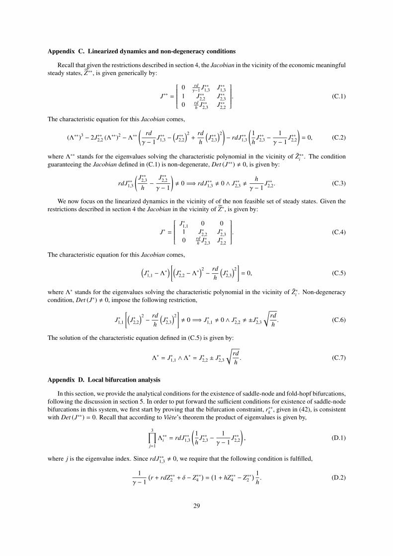
Appendix C. Linearized dynamics and non-degeneracy conditions

Recall that given the restrictions described in section 4, the Jacobian in the vicinity of the economic meaningfulsteady states, Z∗∗, is given generically by:

J∗∗ =

0 rd

γ−1 J∗∗1,3 J∗∗1,31 J∗∗2,2 J∗∗2,30 rd

h J∗∗2,3 J∗∗2,2

. (C.1)

The characteristic equation for this Jacobian comes,

(Λ∗∗)3− 2J∗∗2,2 (Λ∗∗)2

− Λ∗∗(

rdγ − 1

J∗∗1,3 −(J∗∗2,2

)2+

rdh

(J∗∗2,3

)2)− rdJ∗∗1,3

(1h

J∗∗2,3 −1

γ − 1J∗∗2,2

)= 0, (C.2)

where Λ∗∗ stands for the eigenvalues solving the characteristic polynomial in the vicinity of Z∗∗i . The conditionguaranteeing the Jacobian defined in (C.1) is non-degenerate, Det (J∗∗) , 0, is given by:

rdJ∗∗1,3

( J∗∗2,3h−

J∗∗2,2γ − 1

), 0 =⇒ rdJ∗∗1,3 , 0 ∧ J∗∗2,3 ,

hγ − 1

J∗∗2,2. (C.3)

We now focus on the linearized dynamics in the vicinity of of the non feasible set of steady states. Given therestrictions described in section 4 the Jacobian in the vicinity of Z∗, is given by:

J∗ =

J∗1,1 0 01 J∗2,2 J∗2,30 rd

h J∗2,3 J∗2,2

. (C.4)

The characteristic equation for this Jacobian comes,(J∗1,1 − Λ∗

) [(J∗2,2 − Λ∗

)2−

rdh

(J∗2,3

)2]

= 0, (C.5)

where Λ∗ stands for the eigenvalues solving the characteristic polynomial in the vicinity of Z∗i . Non-degeneracycondition, Det (J∗) , 0, impose the following restriction,

J∗1,1

[(J∗2,2

)2−

rdh

(J∗2,3

)2], 0 =⇒ J∗1,1 , 0 ∧ J∗2,2 , ±J∗2,3

√rdh. (C.6)

The solution of the characteristic equation defined in (C.5) is given by:

Λ∗ = J∗1,1 ∧ Λ∗ = J∗2,2 ± J∗2,3

√rdh. (C.7)

Appendix D. Local bifurcation analysis

In this section, we provide the analytical conditions for the existence of saddle-node and fold-hopf bifurcations,following the discussion in section 5. In order to put forward the sufficient conditions for existence of saddle-nodebifurcations in this system, we first start by proving that the bifurcation constraint, r∗∗k , given in (42), is consistentwith Det (J∗∗) = 0. Recall that according to Viète’s theorem the product of eigenvalues is given by,

3∏j=1

Λ∗∗i = rdJ∗∗1,3

(1h

J∗∗2,3 −1

γ − 1J∗∗2,2

), (D.1)

where j is the eigenvalue index. Since rdJ∗∗1,3 , 0, we require that the following condition is fulfilled,

1γ − 1

(r + rdZ∗∗2 + δ − Z∗∗4

)=

(1 + hZ∗∗4 − Z∗∗2

) 1h. (D.2)

29

Substituting the equilibrium expression for Z∗∗2 , (35), and solving in terms of Z∗∗4 , we confirm that r∗∗k isconsistent with the existence of this singularity, Λ∗∗1 = 0, and equal to the equilibrium expression for Z∗∗4

(r∗∗k

),

given in (43),

Z∗∗4 =−

(ρ + δγ +

(γ−1)(ρ−r+δ(γ−1))hrd −

γ−1h

)−

(γ−1)2

hrd − 2γ + 1= Z∗∗4

(r∗∗k

). (D.3)

In three dimensional systems a saddle-node bifurcation occurs if the remaining eigenvalues are of opposite signs,Λ∗∗2 · Λ

∗∗3 < 0. Following (D.2), the characteristic equation is now given by:

−Λ∗∗[(

J∗∗2,2 − Λ∗∗)2−

rdhγ − 1

(J∗∗2,2

)2−

rdγ − 1

J∗∗1,3

]= 0. (D.4)

The eigenvalues at the bifurcation point are thus given by,

Λ∗∗1 = 0 ∧ Λ∗∗2,3 = J2,2 ±

√rdhγ − 1

(J∗∗2,2

)2+

rdγ − 1

J∗∗1,3. (D.5)

The existence of a saddle-node bifurcation can be put in terms of parameter d. We have a saddle-node if

J∗∗1,3 < −h(J∗∗2,2

)2and d > 0; or if J∗∗1,3 > −h

(J∗∗2,2

)2and d < 0. (D.6)

To define analytically the fold-hopf bifurcation point, it is convenient to continue equilibrium from the saddlenode bifurcation defined by r∗∗k . Continuing equilibrium from this point a fold-hopf bifurcation is guaranteed toexist if J∗∗2,2

(r∗∗k

)= 0 ∧ J∗∗2,3

(r∗∗k

)= 0, and provided that d < 0. At this singular point we have a zero eigenvalue,

Λ∗∗1 = 0, and the remaining eigenvalues, Λ∗∗2,3, are given by a pure imaginary conjugate pair, following the resultin (D.5). The expression for the non negative eigenvalues is given by,

Λ∗∗2,3 = ±

√rdγ − 1

J∗∗1,3,rdγ − 1

J∗∗1,3 < 0. (D.7)

To obtain the parameter constraint required for the existence of a codimension two fold-hopf bifurcation, we haveto solve the system given by J∗∗2,2

(r∗∗k

)= 0 ∧ J2,3

(r∗∗k

)= 0. Substituting we obtain,

Z∗∗4(r∗∗k

)=

r + δ + rd1 − hrd

∧ Z∗∗2(r∗∗k

)= 1 + hZ∗∗4

(r∗∗k

). (D.8)

Substituting (D.8) in (D.3), we obtain the second parameter condition, in terms of parameter ρ. This condition isgiven by the following expression,

ρ∗∗ = −

(hrd

γ − 1 + hrd

) [δγ +

(γ − 1) (δ (γ − 1) − r)hrd

−γ − 1

h−

(r + δ + rd1 − hrd

) (−

(γ − 1)2

hrd− 2γ + 1

)]. (D.9)

Appendix E. Geometric analysis of the quadric nullcline surfaces

To classify the nullclines described by the quadrics, Z2 (t) , Z4 (t) = 0, it is first convenient to redefine thesesurfaces as a matrix product, χT Σiχ

T , where χ = [Z2 (t) ,Z4 (t) ,Z1 (t) , 1]. The matrix Σ2 for the nullcline Z2 (t) = 0and its upper sub-matrix, Σ

′

2, are given in general terms, following the notation in Appendix B, by:

Σ2 =

A B

2 0 D2

B2 C 0 E

20 0 0 1

2D2

E2

12 F

and Σ′

2 =

A B2 0

B2 C 00 0 0

. (E.1)

For the nullcline Z4 (t) = 0, Σ4 and Σ′

4, are given by,

Σ4 =

G H

2 0 J2

H2 I 0 K

20 0 0 0J2

K2 0 L

and Σ′

4 =

G H2 0

H2 I 00 0 0

. (E.2)

30

To define these geometric surfaces we need to define the following quantities: (i) det (Σ), det(Σ′); (ii) rank (Σ),

rank(Σ′); and (iii) det

(Σ′

− πI)

= 0. Where π is the eigenvalue solution to the characteristic equation of Σ′

and Ithe identity matrix. For the first quadric surface, Z2 (t) = 0, we obtain the following quantities. When hrd , 1,det (Σ2) = (1 − hrd) /16 and the matrix has full rank, rank (Σ2) = 4, while det

(Σ′

2

)= 0 and rank

(Σ′

2

)= 2. When

hrd = 1, det (Σ2) = 0 and rank (Σ2) = 2, while rank(Σ′

2

)= 1. The surface is a parabolic cylinder when hrd = 1.

Now we need to evaluate the signs of the non negative eigenvalue solutions, π2, for Σ′

2. These are given by,

π2 = 0 ∨ π2 =− 1

2 (rd + h) ±√

14 (rd + h)2 + 1 − rdh

−2. (E.3)

When hrd > 1, we have eigenvalues with the same signs. The quadric Z2 (t) = 0 is: (i) an elliptic paraboloidwhen hrd > 1; and (ii) a hyperbolic paraboloid when hrd < 1. For the second quadric, Z4 (t) = 0, we obtainthe following quantities. When hrd , 1, det (Σ4) = 0 and rank (Σ4) = 3, while det

(Σ′

4

)= 0 and rank

(Σ′

4

)= 2.

When hrd = 1, rank (Σ4) = 3 and rank(Σ′

4

)= 1, the surface is a parabolic cylinder. Now we need to evaluate the

eigenvalues, π4, of Σ′

4. These are given by the following expressions,

π4 = 0 ∨ π4 =

12

(rdh + 1

)±

√14

(rdh + 1

)2+ rd

(rd − 1

h

)−2

. (E.4)

When 0 < rdh < 1, the quadric, Z4 (t) = 0, is an elliptic cylinder54. When hrd < 0 ∧ hrd > 1, the quadric,Z4 (t) = 0, is a hyperbolic cylinder.

References

[1] D. Acemoglu. Introduction to Modern Economic Growth. Princeton University Press, 2009.[2] P. Agenor. Capital inflows, external shocks, and the real exchange rate. Journal of International Money and Finance, 17(5):713–740,

1998.[3] L. Anderlini and D. Canning. Structural stability implies robustness to bounded rationality. Journal of Economic Theory, 101(2):

395–422, 2001.[4] K. Arrow and M. Kurtz. Public Investment, the Rate of Return, and Optimal Fiscal Policy. The John Hopkins University Press, Baltimore,

first edition, 1970.[5] T. Asada, W. Semmler, and A. Novak. Endogenous growth and the balanced growth equilibrium. Research in Economics, 52(2):189–212,

1998.[6] J. Bai and P. Perron. Estimating and testing linear models with multiple structural changes. Econometrica, 66(1):47–48, 1998.[7] J. Bai and P. Perron. Computation and analysis of multiple structural change models. Journal of Applied Econometrics, 18(1):1–22,

2003.[8] P. Bardhan. Optimal Foreign Borrowing, Essays on the Theory of Optimal Economic Growth. Massachusetts Institute of Technology

Press, Cambridge, Massachusetts, first edition, 1967.[9] R. Barro and X. Sala-i-Martin. Economic Growth. MIT press, Massachusetts, second edition, 2004.

[10] C. Bean. Joseph schumpeter lecture the great moderation, the great panic, and the great contraction. Journal of the European EconomicAssociation, 8(2-3):289–325, 2010.

[11] J. Benhabib and K. Nishimura. Indeterminacy and sunspots with constant returns. Journal of Economic Theory, 81(1):58–96, 1998.[12] J. Benhabib, K. Nishimura, and T. Shigoka. Bifurcation and sunspots in the continuous time equilibrium model with capacity utilization.

International Journal of Economic Theory, 4(2):337–355, 2008.[13] P. Brito. Local dynamics for optimal control problems of three-dimensional ode systems. Annals of Operational Research, 89(0):

195–214, 1999.[14] W. Brock and C. Hommes. A rational route to randomness. Econometrica, 65(5):1059–1096, 1997.[15] W. Brock and C. Hommes. Heterogeneous beliefs and routes to chaos in a simple asset pricing model. Journal of Economic Dynamics

and Control, 22(8-9):1235–1274, 1998.[16] W. Brock and J. Scheinkman. Global asymptotic stability of optimal control systems with applications to the theory of economic growth.

Journal of Economic Theory, 12(1), 1976.[17] D. Cass. Optimum growth in an aggregative model of capital accumulation. Review of Economic Studies, 32(3):233–240, 1965.[18] D. Cass and K. Shell. The structure and stability of competitive dynamical systems. Journal of Economic Theory, 12(1):31–70, 1976.[19] P. Chen. Chapter 15- evolutionary economic dynamics: persistent cycles, disruptive technology and the trade-off between stability and

complexity. In K. Dopfer, editor, The Evolutionary Foundations of Economics, pages 472–505. Cambridge University Press, Cambridge,2005.

[20] S. Chen and J. Guo. Velocity of money, equilibrium (in)determinacy and endogenous growth. Journal of Macroeconomics, 30(3):1085–1096, 2008.

[21] A. Chian. Lecture Notes in Economics and Mathematical Systems in Complex Systems Approach to Economic Dynamics (Volume 592).Springer-Verlag, Berlin, first edition, 2007.

54To determine if this elliptic cylinder is real or imaginary the eigenvalues of Σ4 have to be checked. If the non negative eigenvalues haveopposite signs then we have an real elliptic cylinder.

31

[22] G. Corsetti, B. Guimaraes, and N. Roubini. International lending of last resort and moral hazard: A model of IMF’s catalytic finance.Journal of Monetary Economics, 53(3):441–471, 2006.

[23] D. Crommelin, J. Opsteegh, and F. Verhulst. A mechanism for atmospheric regime behavior. Journal of the Atmospheric Sciences, 61(12):1406–1419, 2004.

[24] M. Danca and G. Chen. Bifurcation and chaos in a complex model of dissipative medium. International Journal of Bifurcation andChaos, 14(10):3409–3447, 2004.

[25] C. Deissenberg, G. Feichtinger, W. Semmler, and F. Wirl. History dependence, multiple equilibria, and global dynamics in intertem-poral optimization models. In Economic Complexity: Non-linear Dynamics, Multi-agents Economies, and Learning, ISETE Vol 14,International Symposia in Economic Theory and Econometrics, pages 91–122. Elsevier, 2004.

[26] A. Drazen. Continuous time optimization. Lecture notes, 2007. URL http://econweb.umd.edu/~ture/Files/601/drazen/OptimalCOntrol.pdf.

[27] M. Drelichman and H. J. Voth. Debt sustainability in historical perspective: The role of fiscal repression. Journal of the EuropeanEconomic Association, 6(2-3):657–667, 2008.

[28] J. P. Drugeon. A model with endogenously determined cycles, discounting and growth. Economic Theory, 12(2):349–369, 1998.[29] T. Eicher, S. Schubert, and S. Turnovsky. Dynamic effects of terms of trade shocks: The impact on debt and growth. Journal of

International Money and Finance, 27(6):976–896, 2008.[30] K. French and J. Poterba. Investor diversification and international equity markets. American Economic Review, 81(2):222–226, 1991.[31] G. Fuchs. Structural stability for dynamical economic models. Journal of Mathematical Economics, 2(2):139–154, 1975.[32] P. Gaspard. Generation of a countable set of homoclinic flows through bifurcation. Physics Letters A, 97:1–4, 1983.[33] R. Goodwin. The nonlinear accelerator and the persistence of business cycles. Econometrica, 19(1):1–17, 1951.[34] R. Goodwin. A growth cycle. In C. Feinstein, editor, Socialism, Capitalism and Economic Growth. Cambridge University Press,

Cambridge, 1967.[35] R. Goyal and R. McKinnon. Japan’s negative risk premium in interest rates: The liquidity trap and the fall in bank lending. The World

Economy, 26(3):339–363, 2003.[36] A. Greiner. Endogenous growth cycles-arrow’s learning by doing reconsidered. Journal of Macroeconomics, 18(4):587–604, 1996.[37] A. Greiner and W. Semmler. Saddle path stability, fluctuations, and indeterminacy in economic growth. Studies in Nonlinear Dynamics

& Econometrics, 1(2), 1996.[38] J. Guckenheimer and P. Holmes. Nonlinear Oscillations, Dynamical Systems and Bifurcations of Vector Fields. Springer, first edition,

1983.[39] J. Guckenheimer and P. Holmes. Structurally stable heteroclinic cycles. Mathematical Proceedings of the Cambridge Philosophical

Society, 103:189–192, 1988.[40] F. Hayashi. Tobin’s marginal q and averageq: A neoclassical interpretation. Econometrica, 50(1):213–224, 1982.[41] F. Hilker and H. Malchow. Strange periodic attractors in a prey-predator system with infected prey. Mathematical Population Studies,

13(3):119–134, 2006.[42] A. Homburg and B. Sandstede. Chapter 8- homoclinic and heteroclinic bifurcations in vector fields. In H. Broer, F. Takens, and

B. Hasselblatt, editors, Handbook of Dynamical Systems 3, pages 379–524. Elsevier Science, 2010.[43] C. Hommes and F. Wagener. Complex evolutionary systems in behavioral finance. CeNDEF Working Papers 08-05, Universiteit van

Amsterdam, Center for Nonlinear Dynamics in Economics and Finance, 2008.[44] A. Hurwitz. On the conditions under which an equation has only roots with negative real parts, In: R. Bellman and R. Kalaba, eds.,

Selected Papers on Mathematical Trends in Control Theory. Dover Publications, Inc., New York, first edition, 1964.[45] E. Izhikevich. Synchronization of elliptic bursters. SIAM review, 43(2):315–344, 2001.[46] S. Keen. A monetary minsky model of the great moderation and the great recession. Journal of Economic Behavior and Organization,

forthcoming, 2011.[47] A. Kirman. Complex Economics: Individual and Collective Rationality. Routledge, first edition, 2010.[48] N. Kondratiev. The Major Economic Cycles (in Russian), translated and published as The Long Wave Cycle by Richardson and Snyder,

New York, 1984. Moscow, first edition, 1925.[49] T. Koopmans. On the concept of optimal economic growth, in Econometric Approach to Development Planning. North-Holland Pub-

lishing Co, Amsterdam, first edition, 1965.[50] Y. Kuznetsov. Elements of Applied Bifurcation Theory. Springer-Verlag, New York, second edition, 1998.[51] W. Liu. Criterion of hopf bifurcations without using eigenvalues. Journal of Mathematical Analysis and Applications, 182(1):250–256,

1994.[52] F. Longstaff. The flight-to-liquidity premium in u.s. treasury bond prices. The Journal of Business, 77(3):511–526, 2004.[53] F. Lordon. Cycles et chaos dans un modèle hétérodoxe de croissance endogène. Revue economique, 46(6):1405–1432, 1995.[54] F. Louça. Nikolai kondratiev and the early consensus and dissensions about history and statistics. History of Political Economics, 31(1):

169–206, 1999.[55] R. Lucas. On the mechanics of economic development. Journal of Monetary Economics, 22(1):3–42, 1988.[56] S. Ludvigson and S. Ng. Macro factors in bond risk premia. Review of Financial Studies, 22(12):5027–5067, 2009.[57] R. S. Mackay. Nonlinearity in complexity science. Nonlinearity, 21(12):T273–T281, 2008.[58] P. Mattana, K. Nishimura, and T. Shigoka. Homoclinic bifurcation and global indeterminacy of equilibrium in a two-sector endogenous

growth model. International Journal of Economic Theory, 5(1):25–47, 2009.[59] M. Di Matteo. Economic dynamics as a succession of equilibria: The path travelled by morishima. Technical Report 1209, Department

of Economic Policy, Finance and Development (DEPFID), University of Siena, 2009.[60] L. McKenzie. Turnpike theory. Econometrica, 44(5):841–865, 1976.[61] L. McKenzie. Turnpikes. American Economic Review, 88(2):1–14, 1998.[62] R. Merton. Analytical optimal control theory as applied to stochastic and non-stochastic economics. PhD dissertation, Massachusetts

Institute of Technology, Department of Economics, 1970.[63] M. Miller and L. Zhang. Sovereign liquidity crises: The strategic case for a payments standstill. Economic Journal, 110(460):335–362,

2000.[64] H. Minsky. The financial instability hypothesis. In P. Arestis and M. Sawyer, editors, Handbook of Radical Political Economy. Edward

Elgar, Aldershot, 1992.[65] K. Nishimura. On uniqueness of a steady state and convergence of optimal paths in multisector models of optimal growth with a discount

rate. Journal of Economic Theory, 24(2):157–167, 1981.

32

[66] K. Nishimura and T. Shigoka. Sunspots and hopf bifurcations in continuous time endogenous growth models. International Journal ofEconomic Theory, 2(3-4):199–216, 2006.

[67] T. Palley. A theory of minsky super-cycles and financial crises. Contributions to Political Economy, 30(1):31–46, 2011.[68] M. Peixoto. On structural stability. The Annals of Mathematics, 69(1):199–222, 1959.[69] M. Peixoto. Some examples on n-dimensional structural stability. Proceedings of the National Academy of Sciences of the United States

of America, 45(4):633–636, 1959.[70] P. Perron. The great crash, the oil price shock, and the unit root hypothesis. Econometrica, 57(6):1361–1401, 1989.[71] L. Piscitellia and M. Sportelli. A simple growth-cycle model dysplaying sil’nikov chaos. In Economic Complexity: Non-linear Dynamics,

Multi-agents Economies, and Learning, ISETE Vol 14, International Symposia in Economic Theory and Econometrics, pages 3–30.Elsevier, 2004.

[72] M. Rabinovich and A. Fabrikant. Stochastic self-modulation of waves in nonequilibrium media. Soviet Journal of Experimental andTheoretical Physics, 50:311–317, 1979.

[73] F. Ramsey. A mathematical theory of saving. Economic Journal, 38(152):543–559, 1928.[74] C. Reinhart and K. Rogoff. This time is different: eight centuries of financial folly. Princeton University Press, first edition, 2009.[75] C. Reinhart and M. Sbrancia. The liquidation of government debt. NBER Working Papers 16893, National Bureau of Economic

Research, Inc, 2011.[76] R. Rockafellar. Saddle points of hamiltonian systems in convex lagrange problems having a nonzero discount rate. Journal of Economic

Theory, 12(1):71–113, 1976.[77] P. Romer. Increasing returns and long run growth. Journal of Political Economy, 94(5):1002–1037, 1986.[78] P. Romer. Endogenous technological change. Journal of Political Economy, 98(5):S71–102, 1990.[79] W. Shafer and H. Sonnenschein. Market demand and excess demand functions. volume 2 of Handbook of Mathematical Economics,

chapter 14, pages 671–693. Elsevier, 1993.[80] S. Slobodyan. Indeterminacy and stability in a modified romer model. Journal of Macroeconomics, 29(1):169–177, 2007.[81] H. Sonnenschein. Do walras’ identity and continuity characterize the class of community excess demand functions? Journal of Economic

Theory, 6(4):345–354, 1973.[82] J. Stiglitz and A. Weiss. Credit rationing in markets with imperfect information. American Economic Review, 71(3):393–410, 1981.[83] C. Tresser. Homoclinic orbits for flows in R3. Journal of Physics France, 45(5):837–841, 1984.[84] S. Turnovsky. Methods of Macroeconomic Dynamics. The MIT Press, Cambridge, Massachusetts, first edition, 1995.[85] S. Turnovsky. Fiscal policy and growth in a small open economy with elastic labor supply. Canadian Journal of Economics, 32(5):

1191–1214, 1999.[86] S. Turnovsky. Knife-edge conditions and the macrodynamics of small open economies. Macroeconomic Dynamics, 6(2):307–335, 2002.[87] H. Uzawa. Optimal technical change in an aggregative model of economic growth. International Economic Review, 6(1):18–31, 1965.[88] T. Veblen. Why is economics not an evolutionary science? The Quarterly Journal of Economics, 12(4):373–397, 1898.[89] R. Veneziani and S. Mohun. Structural stability and goodwin’s growth cycle. Structural Change and Economic Dynamics, 17(4):

437–451, 2006.[90] T. Vogelsang and P. Perron. Additional tests for a unit root allowing for a break in the trend function at an unknown time. International

Economic Review, 39(4):1073–1100, 1998.[91] S. Wiggins. Global Bifurcations and Chaos in Applied Mathematical Sciences (Volume 73). Springer-Verlag, Berlin, first edition, 1988.[92] S. Wiggins. Introduction to Applied Nonlinear Dynamical Systems and Chaos in Texts in Applied Mathematics (Volume 2). Springer-

Verlag, Berlin, second edition, 2003.[93] F. Wirl. Stability and limit cycles in a competitive equilibria subject to adjustment costs and dynamic spillovers. Journal of Economic

Dynamics and Control, 26(3):375–398, 2002.[94] W. Zhang. Theory of complex systems and economic dynamics. Nonlinear Dynamics, Psychology, and Life Sciences, 6(2):83–101,

2002.

33