Seminar Ia - I. year of Bologna II. cycle

Nonlinear Oscillators

Author: Ram Dušić HrenMentor: Dr. Simon ŠircaLjubljana, december 2014

Abstract

Linear dynamics is usually obtained only as a first approximation of real physical systems. Inmy seminar I investigate a little further into the vast field of dynamic systems by incorporatingnonlinear effects. By means of a few simple examples of oscillators with nonlinear dynamics, namelythe mathematical pendulum, Duffing oscillator and the Van der Pol oscillator, I show some basicconcepts arising from nonlinearity. In the last chapter I devote a little more attention to the theoryof chaos and describe the Lorenz system.

Contents1 Introduction 1

2 Linear systems 12.1 Equilibrium points and phase plots . . . . . . . . . . . . . . . . . . . . . . . . . . . . . . . 2

3 Nonlinearity 33.1 Lyapunov stability . . . . . . . . . . . . . . . . . . . . . . . . . . . . . . . . . . . . . . . . 33.2 Bifurcations . . . . . . . . . . . . . . . . . . . . . . . . . . . . . . . . . . . . . . . . . . . . 43.3 Chaos . . . . . . . . . . . . . . . . . . . . . . . . . . . . . . . . . . . . . . . . . . . . . . . 4

4 Mathematical pendulum 44.1 Exact solution . . . . . . . . . . . . . . . . . . . . . . . . . . . . . . . . . . . . . . . . . . 5

5 Duffing oscillator 6

6 Van der Pol oscillator 8

7 Lorenz system 97.1 Strange attractor . . . . . . . . . . . . . . . . . . . . . . . . . . . . . . . . . . . . . . . . . 10

8 Conclusion 11

1 IntroductionWhy do nonlinear oscillators deserve additional treatment? Courses in undergraduate physics presentthe foundations and basic concepts of physical description of nature. But when deriving the equationsgoverning it, we more often than not use some drastic simplifications and models that accurately describethe reality only in a limited range of parameters. Usually this is done by linearising the equations. Whilethat often gives us a very good insight and quite suitably describes the phenomena, there is an enormousfield of solutions which we do not see in the linear regime. My goal in this seminar is to present a briefintroduction to the fast-expanding realm of dynamical systems and chaos, with emphasis on the non-linear equations which describe some sort of oscillatory motion. I will not go into details of methods forsolving such equations and derivations, since one could fill a whole library with books on that topic, andstill more would be needed to cover it. Instead, I will present some features that arise from nonlinearity,discuss the solutions and present a compact overview so that the reader can both see the richness outsidelinearity and get familiar with some concrete examples.

2 Linear systemsThroughout most of the seminar I will be dealing with systems of first-order differential equations writtenin vector form as:

x = F(x, t) (1)

where xT = (x, y) and F(x, t)T = (F (x, y, t), G(x, y, t)) [1]. Equations governing physical systems whichI am ultimately interested in are usually second-order equations

x+ f(x, x, t) = 0, (2)

which we break down into a system of two first-order equations by setting F (x, y, t) = y and G(x, y, t) =−f(x, y, t) [1]. In this case y is the velocity. But for the purpose of this chapter, y can be anything.In a linear system, for which the right hand side of equation (1) does not explicitly depend on time, F(x)is a linear function and can be written in matrix notation [2]:

x = A · x (3)

1

We insert the ansatz x(t) = x0 exp(λt) and get an eigenvalue equation for λ. In order for the system tohave nontrivial solutions, det(A−λI) must vanish, from which we get a second-order polynomial equationin λ that is easily solvable [1, 2]:

λ2 − λ trA + detA = 0 =⇒ λ1,2 =trA2

±

√(trA2

)2

− detA (4)

2.1 Equilibrium points and phase plotsWe represent the solutions as parametric curves (trajectories) (x(t), y(t)) in the phase space where t isthe curve parameter.

Critical (equilibrium) points are points where x = 0, or in the case of the linear system solutions ofthe equation [2]

A · x = 0. (5)

Obviously every linear system has an equilibrium point at x = 0. If detA = 0, the origin is also theonly equilibrium point. If detA = 0, equation (5) has infinitely many solutions that form a subspace in aphase plane [2]. An example is a differential equation x = x. This system is in equilibrium if the velocityis zero, so all equilibrium points lie on the x-axis in the phase plane.

Depending on the nature of the eigenvalues λ we can now qualitatively discuss the solutions, whichare of the form x(t) = x01 exp(λ1t) + x02 exp(λ2t) [1]:

• If detA < 0, equation (4) yields two real eigenvalues with opposite signs. Trajectories near theeigenvector with corresponding negative eigenvalue will move toward the equilibrium and the onesnear the eigenvector corresponding to positive eigenvalue will move away from the equilibrium.We get a saddle (Figure 1d). Example of a saddle is the unstable equilibrium of a mathematicalpendulum (position directly above the hinge).

• If 0 < detA < (trA)2

4 we have two real eigenvalues with the same sign, depending on the sign of trA.All points are attracted to or repelled from the equilibrium point. This is called a node (Figures1c and f). Example of a node is the overdamped harmonic oscillator.

• If 0 < (trA)2

4 < detA there are two complex eigenvalues, thus the motion will consist of exponentialgrowth or decay and oscillation. We get a spiral (Figures 1b and e). Example of a spiral is theunderdamped harmonic oscillator.

• Finally, we can have two purely imaginary eigenvalues if trA = 0 and detA > 0. This is a pureharmonic oscillation and the equilibrium point is referred to as the center (Figure 1a). Exampleof a center is the undamped harmonic oscillator

Figure 1: Phase plots of linear systems: (a) a center, (b) a stable spiral, (c) a stable node, (d) a saddle,(e) an unstable spiral and (f) an unstable node [3].

2

Equilibrium point is said to be asymptotically stable if all trajectories converge to it as t → ∞ (allthe eigenvalues of A have negative real parts), unstable if all or ”almost” all (as in the case of saddle)trajectories move infinitely far away from it as t → ∞ (at least one of the eigenvalues of A has positivereal part) and stable if neither is the case, so trajectories are bounded to a finite distance from it (botheigenvalues of A are purely imaginary) [1, 2].

3 NonlinearityIn the previous section we saw that in some sense a critical point of a linear system dictates the flow ofa system. Except in the case of detA = 0, the only critical point was the origin.

A nonlinear system can have any number of critical points from zero to infinity. Different criticalpoints can be of different type, therefore we can no longer talk about a stable or unstable system, sincethe same system can have stable and unstable solutions. Since the phase plot can be influenced by morecritical points of different type, it may look much more complex and, incidentally, chaotic [2].

So in order to find critical points we are looking for solutions of x = y = 0, which immediatelyimplies [1]:

F (x, y) = 0, G(x, y) = 0. (6)

We can expand F (x, y) and G(x, y) around the critical point (x0, y0) in a Taylor series and keep only thelinear term (the constant term is zero because of (6)) to obtain so-called linear variational equations:

dξ

dt=

dF

dx

∣∣∣∣x0

ξ +dF

dy

∣∣∣∣y0

η,dη

dt=

dG

dx

∣∣∣∣x0

ξ +dG

dy

∣∣∣∣y0

η, (7)

where ξ = x − x0 and η = y − y0 [1]. In principle we can then apply the classification described in theprevious section to determine the local shape of the phase plot close enough to the critical point. This isall valid, but it is not that simple. The higher terms that we neglect in the linearisation process, althoughsmall, can play a major role in classification of the critical point. The equation x − x3 + x = 0, forexample, when linearised, exhibits a bounded motion (equilibrium point is a center), while the nonlineardamping term causes it to spiral [1].

So we can conclude that the concept of stability in nonlinear systems is a more complex issue andneeds further investigation. Russian engineer Aleksandr Lyapunov developed a convenient stability theorywhich I will now briefly describe.

3.1 Lyapunov stabilityLet us denote as x(x0, t0; t) a trajectory in the phase space, determined by the initial condition x(t0) = x0.This trajectory is said to be Lyapunov stable if for every arbitrarily small ϵ > 0 we can choose an initialcondition x′

0 close enough to x0 so that |x(x0, t0; t)−x(x′0, t0; t)| < ϵ for every t ⩾ t0. Simply said, points

that start close to each other will stay close to each other. If in addition to that the trajectory startingat x(x′

0, t0; t) converges to x(x0, t0; t) as t → ∞, it is said to be asymptotically stable [4].As will become apparent in the next section on the mathematical pendulum, it is convenient to define

another type of stability, namely the orbital stability. A trajectory may be unstable in the Lyapunovsense, meaning that the distance between the states of a system (points in the phase space) does notremain arbitrarily small as time goes on, but it is still possible that trajectories (curves) remain veryclose together. Thus we say a trajectory x(x0, t0; t) is orbitally stable, if for every arbitrarily small ϵ > 0we can choose x′

0 close enough to x0 so that the distance between x(x′0, t0; t) and the curve plotted by

x(x0, t0; t) remains smaller than ϵ [4].The Lyapunov method of determining the stability of equilibrium points is based on the so-called

Lyapunov function, which is an analog to the potential function from classical mechanics. We willassume without loss of generality that the equilibrium point we are interested in is in the origin (if it isnot, all we need to do is to translate the coordinates, which is trivial). Lyapunov theorem states that ifwe can find a function V (x, t) (the Lyapunov function) with the following properties [4, 5]:

3

V (x, t) ⩾ 0; V = 0 ⇐⇒ x = 0,

V (x, t) = ∂V

∂t+∇V · F(x, t) ⩽ 0,

(8)

then the critical point is stable. If in the second relation a strict inequality holds (except in x = 0), thecritical point is asymptotically stable. It can be shown that an equilibrium point in a nonlinear systemis asymptotically Lyapunov stable if all eigenvalues of the linear variational equations have negative realparts and unstable if there exists at least one eigenvalue of the linear variational equations which has apositive real part. Based on this we can assess when the linear variational equations correctly predict thestability of an equilibrium point [1].

3.2 BifurcationsImagine a dynamic system which depends on a parameter α [4]:

x = F(x, α). (9)

A bifurcation is an event where a smooth change in the parameter α causes a sudden qualitative ortopological change in the behaviour of the system. An example is a change in stability of a critical point.This happens when the eigenvalues of linear variational equations cross the imaginary axis. As we will seelater, bifurcations can give rise to some interesting features, for example, isolated periodic orbits knownas limit cycles can be born out of an equilibrium point [6].

3.3 ChaosChaos is a very interesting feature that a lot of nonlinear systems possess. Note that all the systemswe are dealing with in this seminar are deterministic systems, meaning that in principle a solution isuniquely and exactly determined by the initial conditions. So where does chaos enter? It turns out thatmany solutions are very sensitive to initial conditions. That means that even infinitesimally close startingpoints can diverge to completely different trajectories. In general public, this is known as the butterflyeffect [7]. Regions in phase space that contain points that converge to the same trajectory often havefractal structure. Fractals are mathematical objects that exhibit a self-similar pattern on every scale [8].Usually they are manifolds that are nowhere differentiable. In order to describe fractals, the concept ofdimension has to be extended to non-integer reals. Hausdorff dimension was introduced as a measure ofwhat fraction of space the object takes up [9]. For example, a space-filling curve is topologically a onedimensional object, but can fill out an entire unit square [10]. For regular sets the Hausdorff dimensionequals their topological dimension, which is an integer. Fractals have integer topological dimensions, butthe Hausdorff dimension is non-integer and exceeding the topological.

Edward Lorenz, one of the pioneers of chaos theory whom I will mention again in the last section,described chaos as [7]:

”Chaos is when the present determines the future, but the approximate present does not approximatelydetermine the future.”

Even though nearby points diverge to completely different trajectories, these trajectories are often con-fined to a set called the attractor [11]. These are also often fractals and a great deal of effort has beeninvested into studying the structure of such objects. I will get into a little more detail on chaotic behaviourin some of the examples that follow.

4 Mathematical pendulumAs a first illustration I present a brief overview of the well-known mathematical pendulum. In theundamped and unforced case it is described by the equation [4]

x+ ω20 sinx = 0. (10)

4

We can easily find two sets of equilibrium points: the points (x = 0 ± 2nπ, y = 0) correspond to thestable equilibria with the pendulum hanging directly below the axis and (x = π ± 2nπ, y = 0) are theunstable equilibria with the pendulum directly above the axis. The linear approximation around x = 0yields the equation of the simple harmonic oscillator [4]:

x+ ω20x = 0 (11)

with well known periodic solutions x(t) = C1 exp(iω0t) + C2 exp(−iω0t) and thus (0,0) is a center. Ap-proximating around x = π gives us:

x− ω20x = 0. (12)

As we have seen in the first section, the critical point corresponding to such an equation is a saddle. So wecan get a qualitative picture of how a phase plot would look like. We have centers at (x = 0±2nπ, y = 0)and saddles at (x = π± 2nπ, y = 0). It is indeed so as we can see on Figure 2 showing the exact solutionof equation (10) derived below.

Figure 2: The phase plot of undamped mathematical pendulum. Red arrows indicate the flow of thesystem. We have stable equilibria at (x = 0 ± 2nπ, y = 0) (centers) and unstable equilibria at (x =π ± 2nπ, y = 0) (saddles) [12].

4.1 Exact solutionIf we multiply equation (10) by x and integrate over time we immediately obtain the first integral whichis the total energy:

1

2x2 +

∫ x

0

ω20 sinx′dx′ = const. = ϵ0. (13)

After evaluating the integral, we get:

x = ω0

√2

(cosx− 1 +

ϵ0ω20

). (14)

If we examine this equation we see that −1 < ϵ0ω2

0− 1 < 1 corresponds to periodic solutions (oscillation),

while for ϵ0ω2

0− 1 > 1 the pendulum is rotating. Therefore in the case of oscillation, the amplitude C

follows from cosC = ϵ0ω2

0− 1. Separating dx and dt and integrating gives us

t = t0 +1

ω0

∫ x

0

dx′√2(cosx′ − cosC)

. (15)

This can be further expressed in terms of the elliptic integrals of the first kind F (k, α). Here I will onlymention the result that gives us the relation between the period T (and thus frequency) and amplitudeC:

5

T =4

ω0F

(sin C

2,π

2

). (16)

This is an important result which tells us that frequency is no longer independent of the amplitude aswas true in the linearised case [4].

What about stability? Stability of the trivial solution x(t) = (0, 0) is obvious, since for every radiusϵ we can choose an initial condition so that the orbit is contained entirely within that radius. It is alsoeasy to see the instability of the constant solution x(t) = (π, 0). But how about the periodic solutions?Contrary to what may be intuitive at first, all periodic solutions are Lyapunov unstable! Consider twoorbits close together (that means two oscillations with slightly different amplitudes). We have just learnedthat the frequency also slightly changes. But no matter how small the change, after some time the twooscillations will be out of phase, which means that we cannot choose a starting point close enough sothey stay close enough for all time. They are orbitally stable though [4].

5 Duffing oscillatorThe Duffing oscillator is described by the equation [13]

x+ δx+ βx+ αx3 = γ cosωt. (17)It is one of the simplest nonlinear systems that, under certain conditions, exhibits chaotic behaviour. Itcan be used as an approximation for the damped and forced mathematical pendulum (if we expand sinxup to the order of x3). For β < 0 it describes a mass in a double-well potential, for example, a periodicallyforced steel beam deflected by two magnets, schematically represented in Figure 3 on the left.

Figure 3: Left: An example of an oscillator with a double-well potential. A steel beam is influenced bytwo magnets deflecting it and by an elastic force trying to straighten it. Right: Shapes of E(t), definedin equation (18) for different regions of parameters α, β, δ of equation (17). Examples of trajectories arequalitatively illustrated [13].

We first examine the unforced case, γ = 0. If δ = 0, i.e. there is no damping, the equation can beintegrated in the same fashion as the equation of the mathematical pendulum to obtain

E(t) ≡ 1

2x2 +

1

2βx2 +

1

4αx4 = const. (18)

It is easy to see that in the case of δ > 0, the following relation holds:dE(t)

dt= −δx2. (19)

In that case E(t) satisfies (8) and is therefore a Lyapunov function, which means that the equilibriumpoint at (0,0) is asymptotically stable. At β = 0, a bifurcation occurs; (0,0) becomes unstable and twonew equilibrium points are born (Figure 3 right) [13].

6

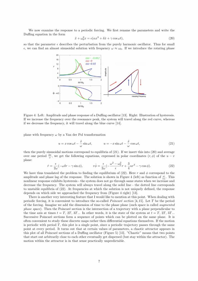
We now examine the response to a periodic forcing. We first rename the parameters and write theDuffing equation in the form

x+ ω20x = ϵ(αx3 + δx+ γ cosωt), (20)

so that the parameter ϵ describes the perturbation from the purely harmonic oscillator. Thus for smallϵ, we can find an almost sinusoidal solution with frequency ω ≈ ω0. If we introduce the rotating phase

Figure 4: Left: Amplitude and phase response of a Duffing oscillator [13]. Right: Illustration of hysteresis.If we increase the frequency over the resonance peak, the system will travel along the red curve, whereasif we decrease the frequency, it will travel along the blue curve [14].

plane with frequency ω by a Van der Pol transformation

u = x cosωt− x

ωsinωt, u = −x sinωt− x

ωcosωt, (21)

then the purely sinusoidal motions correspond to equilibria of (21). If we insert this into (20) and averageover one period 2π

ω , we get the following equations, expressed in polar coordinates (r, ϕ) of the u − vplane:

r =ϵ

2ω(−ωδr − γ sinϕ), rϕ =

ϵ

2ω(−ω2 − ω2

0

ϵr +

3

4αr3 − γ cosϕ). (22)

We have thus translated the problem to finding the equilibrium of (22). Here r and ϕ correspond to theamplitude and phase lag of the response. The solution is shown in Figure 4 (left) as function of ω

ω0. This

nonlinear response exhibits hysteresis - the system does not go through same states when we increase anddecrease the frequency. The system will always travel along the solid line - the dotted line correspondsto unstable equilibria of (22). At frequencies at which the solution is not uniquely defined, the responsedepends on which side we approached the frequency from (Figure 4 right) [13].

There is another very interesting feature that I would like to mention at this point. When dealing withperiodic forcing, it is convenient to introduce the so-called Poincaré section [4, 15]. Let T be the periodof the forcing. Imagine we add the dimension of time to the phase plane (such space is called augmentedphase space). Then the Poincaré section is the intersection of a trajectory with a plane perpendicular tothe time axis at times t = T , 2T , 3T ... In other words, it is the state of the system at t = T , 2T , 3T ...Successive Poincaré sections form a sequence of points which can be plotted on the same plane. It isoften convenient to study these discrete maps rather then differential equations themselves. If the motionis periodic with period T , this plot is a single point, since a periodic trajectory passes through the samepoint at every period. It turns out that at certain values of parameters, a chaotic attractor appears inthis plot of all Poincaré sections of a Duffing oscillator (Figure 5) [13]. ”Chaotic” means that two pointsthat start out arbitrarily close to each other eventually get dispersed (but stay within the attractor). Themotion within the attractor is in that sense practically unpredictable.

7

Figure 5: Successive Poincaré sections plot of the Duffing oscillator for α = 1, β = 0, δ = 0.05 andγ = 7.5, showing a chaotic attractor. Each point on the plot corresponds to one Poincaré section. It isclear from the plot that motion is not periodic, but again not random, since all the points form a welldefined shape [13].

6 Van der Pol oscillatorVan der Pol oscillator is governed by the equation [16]:

x− µ(1− x2)x+ x = 0. (23)

It is a self-oscillating system discovered by a dutch engineer Balthasar van der Pol in some electricalcircuits involving triodes. Since then it has been used to model numerous systems, including the humanheart [17]. It also exhibits nonlinear features like hysteresis and chaos under certain conditions, butit is best known for the self-oscillation orbit known as a stable limit cycle. As the parameter µ getslarger, it becomes a relaxation oscillator, meaning the oscillation consists of a slow asymptotic movementand sudden discontinuous jumps (such oscillators are sometimes used to produce square or trianglewavefunctions) [16].

Figure 6: Left: The limit cycles of the van der Pol oscillator for different values of µ with x on thehorizontal axis and x on the vertical [16]. Right: The waveform of the van der Pol oscillator for µ = 10,showing relaxation oscillations [18].

A quick glimpse at the equation (23) reveals the following: given that µ > 0, for x2 < 1, the dampingterm is negative, thus (0,0) is an unstable focus or node. But for x2 > 1 the damping term is positive,

8

meaning amplification, which implies somewhere in between is a stable self-sustaining solution [1, 18].That is the stable limit cycle. So let us examine how that happens. The bifurcation obviously occursat µ = 0. For µ ≪ 1, we expect an almost sinusoidal oscillation, since the nonlinear damping is a smallperturbation to the harmonic oscillator. In this case it is convenient to break down equation (23) to [18]:

x = µ

(x− 1

3x3 − y

), y =

x

µ. (24)

Similarly to the approach we used with the Duffing oscillator, we transform to a rotating plane withthe unit frequency of a non-perturbed oscillator, insert the transformed coordinates into the dynamicequation and average over one period to obtain [18]:

r =µ

8r(4− r2). (25)

This equation has an unstable equilibrium at r = 0 and stable equilibrium at r = 2. Therefore, for smallµ the limit cycle is almost a circle with radius 2.

When µ gets larger, the circle becomes deformed. Because the damping term changes sign at x = ±1,the system is being repelled from equilibrium for |x| < 1 and drawn back to it for |x| > 1. As µ grows,these jumps become larger [18]. The deformation of the limit cycle with increasing µ is shown in theFigure 6 on the left. At large values of µ, this produces a typical relaxation waveform, represented inFigure 6 on the right.

7 Lorenz systemIn this last chapter I would like to present few concepts from chaos theory that I found very interesting.The Lorenz attractor (Figure 7), forming under certain values of parameters in the Lorenz system, is oneof the most famous images in chaos theory which is why this system serves well as an illustration [19,22].

Figure 7: The Lorenz attractor [20].

The Lorenz system is a system of three equations [19,20]:

x = σ(y − x),

y = x(ρ− z)− y,

z = xy − βz.

(26)

Edward Lorenz proposed it as a drastically simplified model of convection in the atmosphere. It alsohas a quite simple exact physical realisation; these equations turn out to exactly describe the so-calledchaotic waterwheel: a circular frame with cups attached to it, which leak water from the bottom and

9

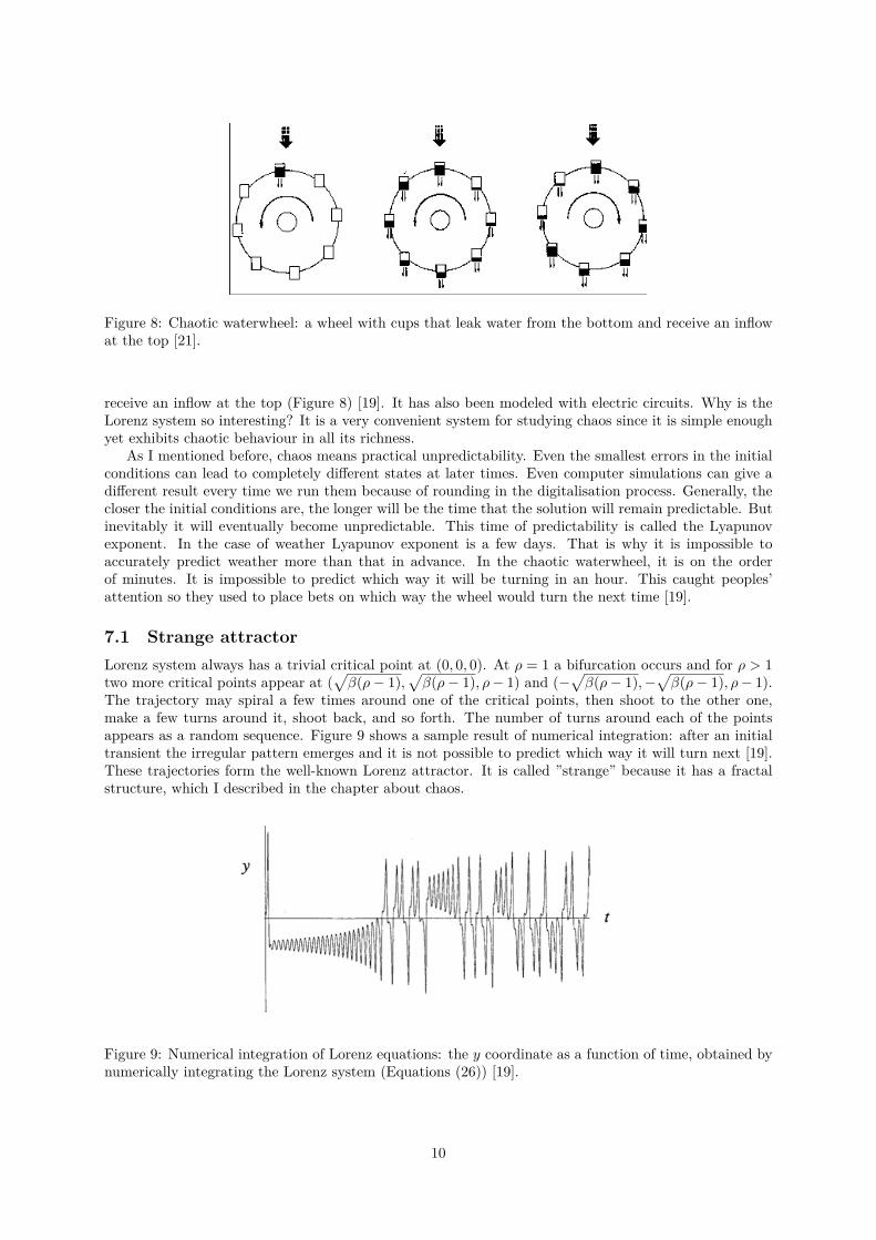
Figure 8: Chaotic waterwheel: a wheel with cups that leak water from the bottom and receive an inflowat the top [21].

receive an inflow at the top (Figure 8) [19]. It has also been modeled with electric circuits. Why is theLorenz system so interesting? It is a very convenient system for studying chaos since it is simple enoughyet exhibits chaotic behaviour in all its richness.

As I mentioned before, chaos means practical unpredictability. Even the smallest errors in the initialconditions can lead to completely different states at later times. Even computer simulations can give adifferent result every time we run them because of rounding in the digitalisation process. Generally, thecloser the initial conditions are, the longer will be the time that the solution will remain predictable. Butinevitably it will eventually become unpredictable. This time of predictability is called the Lyapunovexponent. In the case of weather Lyapunov exponent is a few days. That is why it is impossible toaccurately predict weather more than that in advance. In the chaotic waterwheel, it is on the orderof minutes. It is impossible to predict which way it will be turning in an hour. This caught peoples’attention so they used to place bets on which way the wheel would turn the next time [19].

7.1 Strange attractorLorenz system always has a trivial critical point at (0, 0, 0). At ρ = 1 a bifurcation occurs and for ρ > 1two more critical points appear at (

√β(ρ− 1),

√β(ρ− 1), ρ− 1) and (−

√β(ρ− 1),−

√β(ρ− 1), ρ− 1).

The trajectory may spiral a few times around one of the critical points, then shoot to the other one,make a few turns around it, shoot back, and so forth. The number of turns around each of the pointsappears as a random sequence. Figure 9 shows a sample result of numerical integration: after an initialtransient the irregular pattern emerges and it is not possible to predict which way it will turn next [19].These trajectories form the well-known Lorenz attractor. It is called ”strange” because it has a fractalstructure, which I described in the chapter about chaos.

Figure 9: Numerical integration of Lorenz equations: the y coordinate as a function of time, obtained bynumerically integrating the Lorenz system (Equations (26)) [19].

10

8 ConclusionI made a brief voyage through nonlinear dynamics, the field that really emerged with the birth of powerfulcomputers. There are really not many analytical tools we can use to combat these complicated systems,but I found that very much can be learned from qualitative studies. Almost nothing in nature is linear soit is important to try to understand this field in order to gain a deeper insight to the beauty of Nature.

References[1] R. H. Rand, Lecture Notes on Nonlinear vibrations, version 52, Cornell University, 2005

(http://www.math.cornell.edu/ rand/randdocs/nlvibe52.pdf)

[2] http://www.math.psu.edu/tseng/class/Math251/Notes-PhasePlane.pdf, stran obiskana 6.9.2015

[3] http://lalashan.mcmaster.ca/theobio/DushoffLab/index.php/3MB3-Lecture3, stran obiskana6.9.2015

[4] P. Hagedorn, Non-Linear Oscillations, Second Edition, Clarendon Press, Oxford, 1988

[5] http://en.wikipedia.org/wiki/Lyapunov_stability, stran obiskana 6.9.2015

[6] http://en.wikipedia.org/wiki/Bifurcation_theory, stran obiskana 6.9.2015

[7] http://en.wikipedia.org/wiki/Chaos_theory, stran obiskana 6.9.2015

[8] http://en.wikipedia.org/wiki/Fractal, stran obiskana 6.9.2015

[9] http://en.wikipedia.org/wiki/Hausdorff_dimension, stran obiskana 6.9.2015

[10] http://en.wikipedia.org/wiki/Space-filling_curve, stran obiskana 6.9.2015

[11] https://en.wikipedia.org/wiki/Attractor, stran obiskana 6.9.2015

[12] https://mathematicalgarden.wordpress.com/2009/03/29/nonlinear-pendulum/, stran obiskana6.9.2015

[13] http://www.scholarpedia.org/article/Duffing_oscillator, stran obiskana 6.9.2015

[14] http://large.stanford.edu/courses/2007/ph210/hong1/images/f4big.jpg, stran obiskana 6.9.2015

[15] https://en.wikipedia.org/wiki/Poincare_map, stran obiskana 6.9.2015

[16] https://en.wikipedia.org/wiki/Van_der_Pol_oscillator, stran obiskana 6.9.2015

[17] S.R.F.S.M. Gois, M.A. Savi, An analysis of heart rhythm dynamics using a three-coupled oscillatormodel; Chaos, Solitons and Fractals 41 (2009) 2553?2565

[18] http://www.scholarpedia.org/article/Van_der_Pol_oscillator, stran obiskana 6.9.2015

[19] S.H.Strogatz, Nonlinear Dynamics and Chaos With Applications to Physics, Biology, Chemistry andEngineering, Perseus Books, 1994

[20] https://en.wikipedia.org/wiki/Lorenz_system, stran obiskana 6.9.2015

[21] http://www.ace.gatech.edu/experiments2/2413/lorenz/fall02/, stran obiskana 6.9.2015

[22] http://mathworld.wolfram.com/LorenzAttractor.html, stran obiskana 6.9.2015

11