APS/123-QED

Nonlinear light scattering from clusters and single particles

Jerry I. Dadap1, Hilton B. de Aguiar2, and Sylvie Roke2∗

1Department of Applied Physics and Applied Mathematics,

Columbia University, New York, New York 10027, USA

2Max-Planck Institute for Metals Research,

70569 Stuttgart, Germany Fax: +49-711-6893612

(Dated: April 14, 2009)

Abstract

We present sum-frequency-scattering experiments on colloidal dispersions with various concen-

trations and in different scattering geometries. At small scattering angles, large fluctuations are

observed in the intensity of the scattered sum-frequency photons. By considering the angular de-

pendence of the signal, the particle concentration dependence, and the surface vibrational spectra

of the particle, we have determined that the fluctuations are caused by scattering from clusters of

particles. We further demonstrate that dynamic nonlinear light scattering may be used to measure

the size of the correlated particle clusters.

PACS numbers: 82.70.Dd,42.65.-k,68.60.-p,78.68.+m

∗Electronic address: roke@mf.mpg.de

1

I. INTRODUCTION

For the past four decades, second-order nonlinear optical measurements such as Second-

Harmonic Generation (SHG) and Sum-Frequency Generation (SFG) have been used to probe

the planar surfaces of materials whose bulk media are centrosymmetric (see e.g. [1–7]).

The interface sensitivity of these techniques arises from the fact that within the dipole

approximation, SHG or SFG is forbidden from the bulk of centrosymmetric media. At the

interface, however, the inversion symmetry is broken thereby allowing the SHG and SFG

processes.

Although second harmonic light scattering was observed in a surface-enhanced Hyper-

Raman scattering experiment in 1982 [8], it has been performed only with the aim of directly

measuring surface properties in 1996 via surface SHG scattering [9]. Within the last 13

years, a rapidly growing number of publications reported on second-order Nonlinear Light

Scattering (NLS) from small particles to probe their surfaces. Second-Harmonic Scattering

(SHS) was used to probe (electronic) transitions on particle surfaces in condensed media

[9–19] as well as liposomes in solution [20]. Vibrational Sum-Frequency Scattering (SFS)

was performed to measure the molecular interface structure and its solvent dependence on

colloids in solution [21–23], as well as inclusions in biodegradable polymer microspheres

[24–26].

In such experiments, however, it is possible to induce competing incoherent nonlinear light

scattering processes, such as Hyper-Rayleigh Scattering (HRS), Parametric Light Scatter-

ing (PLS), Two-Photon Fluorescence (TPF), and hyper-Raman scattering [27]. The energy

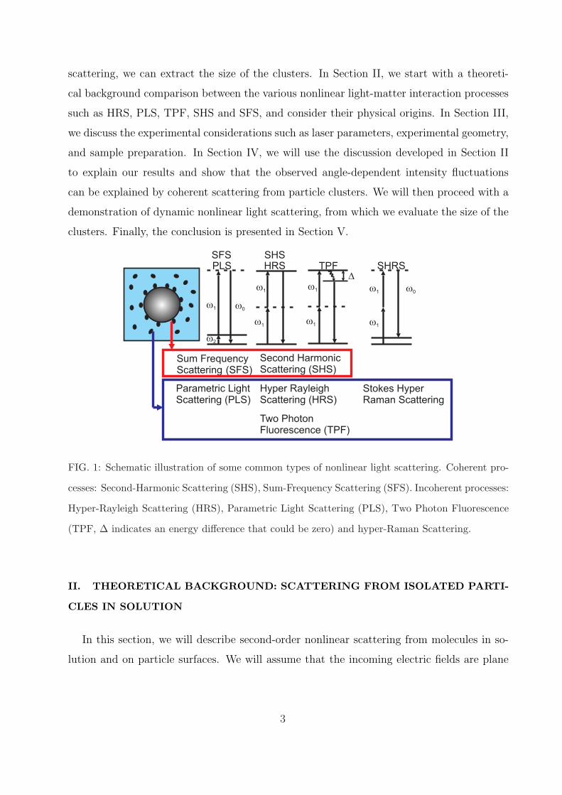
schemes of these processes are illustrated in Fig. 1. In addition, a dispersion of colloids is a

dynamic system in which particles can collide, aggregate, and diffuse. The effects of correla-

tions from such processes have not yet been considered. Thus, a detailed understanding of

the origins of these processes is crucial to the development and the rapid growth of diverse

applications of NLS in various chemical and physical systems.

In this Article, we present sum-frequency spectroscopy scattering measurements per-

formed in different geometries on dispersions with low and high particle concentrations. By

considering several coherent (SHS and SFS) and incoherent nonlinear light scattering (such

as HRS, PLS, TPF) processes, we demonstrate that clusters can dramatically influence the

signal at certain scattering angles. In addition, we show that using dynamic nonlinear light

2

scattering, we can extract the size of the clusters. In Section II, we start with a theoreti-

cal background comparison between the various nonlinear light-matter interaction processes

such as HRS, PLS, TPF, SHS and SFS, and consider their physical origins. In Section III,

we discuss the experimental considerations such as laser parameters, experimental geometry,

and sample preparation. In Section IV, we will use the discussion developed in Section II

to explain our results and show that the observed angle-dependent intensity fluctuations

can be explained by coherent scattering from particle clusters. We will then proceed with a

demonstration of dynamic nonlinear light scattering, from which we evaluate the size of the

clusters. Finally, the conclusion is presented in Section V.

Sum FrequencyScattering

Second HarmonicScattering (SHS)

Parametric LightScattering (PLS)

(SFS)

Stokes HyperRaman Scattering

Hyper RayleighScattering (HRS)

w1

w1

w1

w1

w1 w0

w0

w2

SFS SHSPLS HRS TPF SHRS

w1

w1

D

Two PhotonFluorescence (TPF)

FIG. 1: Schematic illustration of some common types of nonlinear light scattering. Coherent pro-

cesses: Second-Harmonic Scattering (SHS), Sum-Frequency Scattering (SFS). Incoherent processes:

Hyper-Rayleigh Scattering (HRS), Parametric Light Scattering (PLS), Two Photon Fluorescence

(TPF, ∆ indicates an energy difference that could be zero) and hyper-Raman Scattering.

II. THEORETICAL BACKGROUND: SCATTERING FROM ISOLATED PARTI-

CLES IN SOLUTION

In this section, we will describe second-order nonlinear scattering from molecules in so-

lution and on particle surfaces. We will assume that the incoming electric fields are plane

3

waves of the form

E1(r, t) = E1ei(k1·r−ω1t) (1)

E2(r, t) = E2ei(k2·r−ω2t)

where ω1 and ω2 are the angular frequencies, and k1 and k2 are the wave vectors. In gen-

eral both coherent and incoherent scattering processes that lead to the emission of sum

frequency photons with wave vector k0 and frequency ω1 + ω2 = ω0 can take place. Co-

herent optical scattering refers to the electric field scattered from different locations arising

from a superposition of nonlinear polarization sources that have a defined phase relation.

Incoherent nonlinear scattering refers to additional radiation due to local fluctuations in

the electric dipole moment that may arise from, e.g., dephasing or orientational fluctuation.

Consequently for the coherent process, the radiated power scales as N2, whereas for the

incoherent process, the power scales as N , where N is the number density of the dipole

sources, e.g., molecules.

A. Incoherent nonlinear light scattering from molecules in solution

From a historical point of view, the case of the incoherent second-order nonlinear optical

scattering has been well studied beginning with the work of Terhune et al. [28] and further

developed by others [29–34]. For a general three-photon scattering process arising from

randomly oriented non-correlated (NC) molecules, (which includes PLS, HRS, TPF, as well

as hyper-Raman scattering processes) the measured intensity (INC) can be expressed in the

form

INC = ε∗αIαβεβ (2)

Iαβ = AαiAβlIil (3)

Iil = NG〈β(2)ijkβ

(2)∗lmn〉E1,jE2,kE

∗1,mE∗

2,n (4)

where εα (α= θ or φ) is the component of the unit polarization vector ε of the second-

harmonic or sum-frequency signal detected along the r direction, Aαi is the element of the

transformation matrix from the Cartesian reference frame to the polar coordinates reference

frame, [28, 30, 31, 33, 34], β(2)ijk is the molecular hyperpolarizability, and G is a constant

quantity that depends on the geometrical parameters of the detection system. Note that all

4

subscript indices refer to the laboratory frame. The angular brackets denote orientational

averaging due to the random orientation of the molecules.

The various incoherent scattering processes have different polarization properties. Al-

though their directionalities (radiation patterns) are also distinctive, in general scattered

photons can appear in all directions. This can be seen directly from the term 〈β(2)ijkβ

(2)∗lmn〉, a

six-ranked tensor, which governs the overall scattering process. For example, for a molecule

having a general symmetry, there is a maximum of 15 measurable quantities for PLS, which

correspond to the number of the rotational invariants derived from the decomposition of the

〈β(2)ijkβ

(2)∗lmn〉 tensor [31, 33, 34]. For a non-resonantly excited SF-TPF process, this number

reduces to 7 [32]. These numbers of observables are further decreased when considering

the corresponding light generating processes of HRS and SH-TPF. From these observations,

these various processes have the potential to be uniquely identified based on their polariza-

tion properties and their radiation patterns. Another significant difference between these

incoherent processes lies in their response time. In particular, PLS and HRS are instan-

taneous processes while the TPF is a delayed process. For the case of TPF, two-photon

absorption occurs in a molecule, which later fluoresces from the same orientation and may

occur at other frequencies. An intermediate relaxation to a fluorescing state may occur be-

tween these two effects (see Fig. 1). Thus in the TPF process, the total process may occur

on a vibrational time scale but can also take much longer. Furthermore, the two-photon

absorption and fluorescence are two independent quantum mechanical processes that do not

interfere with each other. It should be noted that higher-order processes such as three-

photon absorption and subsequent fluorescence might also contribute to the SH or SF signal

[31].

Various schemes have been developed in order to distinguish between these incoherent

processes such as spectral separation [35], direct temporal separation [36], and temporal

separation in the Fourier domain [37]. Polarization dependencies of the PLS [38] and HRS

[39, 40] measurements have been demonstrated previously.

B. Coherent nonlinear light scattering from a particle

Here, we consider only molecules adsorbed on spherical particles (with radius a and

refractive index n1), because most materials consist of isotropic material and experiments

5

on planar substrates have shown that very often the isotropic bulk response can be neglected.

For coherent NLS from a non-isotropic bulk see e.g. Ref. [24]. For the case of a sphere,

embedded in a medium with refractive index n2, the coherently emitted nonlinear signals

arise from its surface because of the strong orientational correlation of the adsorbed molecules

due to the selectivity of the molecular adsorption or binding process. There is a definite

phase relationship between the dipole sources that are located at different locations and, as a

consequence, this may give rise to coherent signal. At the surface of a particle, orientational

correlation between neighboring molecules may give rise to an effective local nonlinear optical

response, which may be described by the nonlinear surface susceptibility χ(2)s . Various

theoretical formalisms of SHG and SFG from single spheres have been developed [21, 41–

52]. The nonlinear polarization of the SF signal arising from molecules located at the surface

of a sphere is denoted by

P(2)(ω1 + ω2, r′) = χ(2)

s : E1(r′)E2(r

′) (5)

The tensor quantity χ(2)s is related to the hyperpolarizability tensor β(2) according to the

equation [1]:

χ(2)s,ijk = Ns〈TiaTjbTkc〉β(2)

abc (6)

where Ns is the molecular surface density, Tia is an element of the transformation matrix T

that transforms from the molecular frame to the particle surface reference frame, and β(2)abc is

an element of the hyperpolarizability tensor in the molecular frame. In reality, one needs to

calculate the electric fields at the location of the dipole source r′ as indicated in Eq. 5 prior

to calculation of the nonlinear polarization P(2)(ω1 + ω2, r′). After obtaining the nonlinear

polarization, the relevant boundary conditions are applied [45], which then yield the SH or

SF field E(ω1+ω2, r′). The solution to the exact and general problem is outlined in Ref. [53]

for SHS where it is applied to small particles in the Rayleigh limit and in [52], where it is

applied for SFS using the principle of time reversal. Because of the sheer complexity of the

problem, approximations such as the Rayleigh-Gans-Debye (RGD) [21, 43, 49, 50, 53–55],

and Wentzel-Kramers-Brillouin (WKB) [49, 56] methods have been proposed. See Ref. [57]

for an overview.

Here, we consider only the RGD method, which has been shown to work for silica particles

in solution with radii up to 650 nm and a refractive index difference at the SF wavelength

of 0.03 [21, 49]. Within the RGD model, the internal field is assumed to be the same as

6

the incident field. This model is roughly valid under two conditions: (1) |m − 1| ¿ 1,

where m= n1/n2 and (2) 4πa|m− 1|/λ ¿ 1, where λ is the smaller of the two wavelengths

corresponding to ω1 or ω2. This model has been shown to be quite successful in describing

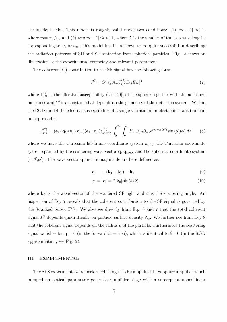
the radiation patterns of SH and SF scattering from spherical particles. Fig. 2 shows an

illustration of the experimental geometry and relevant parameters.

The coherent (C) contribution to the SF signal has the following form:

IC = G′|ε∗αAαiΓ(2)ijkE1jE2k|2 (7)

where Γ(2)ijk is the effective susceptibility (see [49]) of the sphere together with the adsorbed

molecules and G′ is a constant that depends on the geometry of the detection system. Within

the RGD model the effective susceptibility of a single vibrational or electronic transition can

be expressed as

Γ(2)ijk = (ei · ql)(ej · qm)(ek · qn)χ

(2)s,αβγ

∫ 2π

0

∫ π

0

BiαBjβBkγeiqa cos (θ′) sin (θ′)dθ′dφ′ (8)

where we have the Cartesian lab frame coordinate system ei,j,k, the Cartesian coordinate

system spanned by the scattering wave vector q, ql,m,n and the spherical coordinate system

(r′,θ′,φ′). The wave vector q and its magnitude are here defined as:

q ≡ (k1 + k2)− k0 (9)

q = |q| = 2|k0| sin(θ/2) (10)

where k0 is the wave vector of the scattered SF light and θ is the scattering angle. An

inspection of Eq. 7 reveals that the coherent contribution to the SF signal is governed by

the 3-ranked tensor Γ(2). We also see directly from Eq. 6 and 7 that the total coherent

signal IC depends quadratically on particle surface density Ns. We further see from Eq. 8

that the coherent signal depends on the radius a of the particle. Furthermore the scattering

signal vanishes for q = 0 (in the forward direction), which is identical to θ= 0 (in the RGD

approximation, see Fig. 2).

III. EXPERIMENTAL

The SFS experiments were performed using a 1 kHz amplified Ti:Sapphire amplifier which

pumped an optical parametric generator/amplifier stage with a subsequent noncollinear

7

k1

k0 q

k2

r' f'

q'

qk2+ =k k1 0

0b

exey

ez

qy qx

qz

s p

lan

e

p plane

FIG. 2: Illustration of the in-plane scattering geometry of the experiments, indicating the k-vectors

of the incoming beam (k1 and k2) and the scattered sum frequency beam k0, the scattering wave

vector (q), and the scattering angle (θ). Beams polarized parallel to the plane of incidence are

defined as p-polarized, while beams with an oscillating field in the y-direction are indicated as

s-polarized. The direction k1 + k2 is called the forward direction (θ=0).

difference frequency generation stage (TOPAS, Light Conversion) (see Ref. [21] for Figs. 3 -4

and Ref. [58] for Fig. 6). The pulse bandwidths and energies are given in the respective figure

captions. The selectively p-polarized IR and VIS pulses were incident under a relative angle

of 15◦ (β) and focused down to a ∼0.4 mm beam waist. The scattered light was collimated

with a lens, p-polarization selected and dispersed onto an intensified charge coupled device

(CCD) camera. The angular resolution was controlled by an aperture placed in front of

the collimating lens. The samples consist of stearic alcohol (C18H37OH)-coated [59] silica

particles [60] dispersed in CCl4 (99.9%, Baker Analyzed) with a radius a = 342 nm ± 36

nm, as measured with Transmission Electron Microscopy (TEM) [21]. The colloid volume

fractions was 5 or 25 v.v.%. The sample cell consists of 2 CaF2 plates separated by a 1 mm

teflon spacer. The scattering geometry is illustrated in Fig. 2.

IV. RESULTS AND DISCUSSION

We have performed vibrational SFS measurements on colloidal dispersions with short

integration times and in different scattering angles, and observe strong fluctuations in the

scattered intensity. We have investigated the effect of clustering further by increasing the

8

colloid volume fraction from 5 v.v% to 25 v.v%.

A. Angular dependence

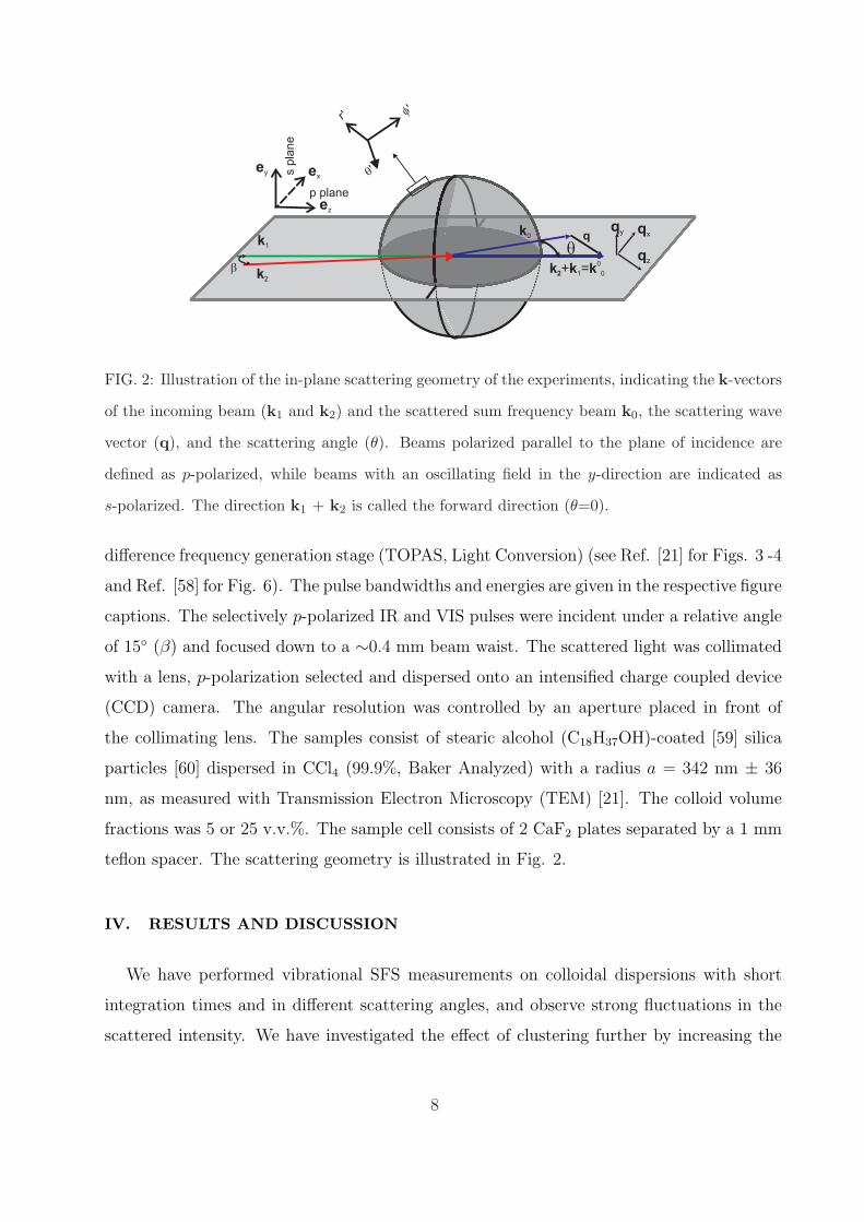
Fig. 3a shows 100 stacked vibrational SFS spectra recorded at scattering angle θ = 63◦.

A single spectrum is presented in panel b. The integration time per spectrum was 6 s, so

that the total time lapse is 600 s. Panel c shows the integrated spectral intensity versus time.

It can be seen that at large scattering angle the spectral intensity is low and constant. In

80

60

40

20

0300028002600

900

4

3

2

1

0

SF

G I

nte

nsity (

a.u

.)

IR Wavenumber (cm )-1

Sp

ectr

um

Nu

mb

er

I(a

.u.)

SF

G

x 103

q=63o

0 1

Inte

gra

ted

I(a

.u.) x

10

SF

G

6

a

b

c

FIG. 3: Vibrational SFS spectra of a 5 v.v.% colloidal dispersion, measured with 10 µJ (120 fs) IR

pulses centered at 2900 cm−1 and 3.0 µJ, 800 nm visible (VIS) pulses with a 10 cm−1 bandwidth,

at a scattering angle of θ = 63◦. (a) Image array of 100 spectra. The color scale indicates the

intensity. (b) One 6 s spectrum (number 83). (c) The integrated intensity per spectrum. The

angular resolution was 12◦.

contrast, in Fig. 4 the same type of experiment is shown except that the detection angle is

closer to the forward direction at θ = 16◦. Here, we observe large fluctuations (”hot spots”)

in the intensity as a function of time.

The observed intensity fluctuations can be due to coherent scattering from large objects,

like clusters but also in principle due to incoherent light scattering. As described in section

II, we can distinguish between these processes by analyzing the angular dependence of the

9

signal and the spectral content. TPF of the double IR or VIS frequency typically occurs in

a different frequency range, which makes it easily distinguishable. While it could be playing

a role in similar SHS experiments, TPF does not occur in these SFS experiments since there

are no electronic transitions that match any combination of incoming beams. PLS from the

solution molecules can be a candidate for signal distortion because the radiation pattern for

PLS is (like that of HRS) relatively isotropic. However, since the generation of PLS typically

requires a large dipole moment [27, 38] it is not a likely source for the strong fluctuations

that were observed. Since there was no signal from a neat solution we can exclude PLS as

a source for scattering.

4

3

2

1

0

SF

G I

nte

nsity (

a.u

.)

80

60

40

20

03000290028002700

5000

0

Sp

ectr

um

Nu

mb

er

IR Wavenumber (cm )-1

x 0.1

I(a

.u.)

SF

G

x 104

q=16o

43210

a

b

c

Inte

gra

ted I

(a.u

.) x 1

0S

FG

6

FIG. 4: Vibrational SFS spectra of a 5 v.v.% colloidal dispersion, measured with 10 µJ (120 fs) IR

pulses centered at 2900 cm−1 and 3.0 µJ, 800 nm visible (VIS) pulses with a 10 cm−1 bandwidth, at

a scattering angle of θ = 16◦. (a) Image array of 100 spectra. The color scale indicates the intensity.

(b) Two 6 s spectra corresponding to a hot spot (number 20, top) and one that corresponds to

scattering from 342 nm colloids (number 19, bottom). (c) The integrated intensity per spectrum.

The angular resolution was 12◦. It can be seen that there are some large fluctuations (hot spots)

in the intensity.

This means that the observed hot spots could come from a coherent surface scattering

process. In order to get more insight into the source of the scattering we have analyzed

10

the spectral features of both the fluctuating high intensity and the constant low intensity

signals. Fig. 5 (left panel) shows the average SFS spectrum of the hot spots present in Fig.

4, compared to the average spectrum of the constant low intensity signal. It can be seen that

both the spectral intensity as well as the spectral shape are completely different. Spectral

fits were made according to the well-known description of vibrational sum-frequency spectra,

so that the spectral shape could be described by the following expressions (see e.g. [21, 61]):

ISFG(ω0, θ) ∝ |Γ(2)|2; Γ(2) =∑

n

Γ(2)n + ANR(θ)Γ

(2)NRei∆φ; Γ(2)

n ∝ An(θ)

(ω − ω0n) + iΥn

, (11)

where ANR refers to the angle dependent amplitude of the non-resonant background with

relative phase ∆φ, n refers to a vibrational mode, with resonance frequency ω0n, amplitude

An and damping constant Υn. Both the resonant and non-resonant amplitudes are angle

dependent [57]. The averaged spectra of the small intensity signal can be attributed to single

particles and could be fit with the resonances of the surface bound stearyl groups without

assuming a non-resonant contribution. For the fit, both the symmetric CH3 (A2885 = 11.4)

and CH2 stretch modes (A2850 = 20.4) and the asymmetric CH2 (A2911 = 14.6) and CH3

stretch (A2972 = 2.16) modes were needed as well as the Fermi resonance (A2932 = 10.3).

These fits were almost identical to the ones presented in Ref. [21] and the presence of all

these modes indicates that the surface chains are disordered (as was shown earlier [21, 22]).

The spectral signature of the averaged hot spot spectrum (Fig. 5, upper trace) is remark-

ably different and could not be described without an appreciable amount of non-resonant

background (ANR = 2, ∆φ = 100◦). Additionally the symmetric CH2 and CH3 stretch

amplitudes decreased with a factor of 2. The asymmetric CH3 and CH2 modes increased

with a factor of 2 and 5 respectively, while the amplitude of the Fermi resonance changed

very little. These changes indicate that the source of the hot spot still has alkane chains

attached to it, although the average conformational distribution is different. Thus, the ob-

ject giving rise to hot spots are composed of dispersed colloids. Provided the non-resonant

signal depends on the amount of bulk material in the object, the increase in non-resonant

signal points towards an increase in bulk (silica) material. Further, we observe only hot

spots when the scattering angle is in the range ∼ −30◦ ≤ θ ≤∼ 30◦. Using Eqs. 7 and 8

we have calculated the scattering pattern within the RGD approximation for spheres with

different sizes. Fig. 5 (right panel) shows calculated angular distributions (using the non-

linear RGD model in combination with the parameters for stearyl-coated silica particles as

11

15

10

5

0-50 0 50

Scattering angle (degrees)q

a =342 nma = 3.4 mm

a =34 mm

Inte

nsity (

a.u

.) x10-4

x10-6

SF

G I

nte

nsity (

a.u

.)

Wavenumber (cm )-1

x 0.1

10

8

6

4

2

03200300028002600

FIG. 5: Left: Averaged normal (single particle) spectra (red trace) and averaged hot spot (blue

trace) taken at θ = 16◦. The spectral shape as well as the intensity are remarkably different.

The straight lines are fits to the data according to the description in the text. The Lorentzian

peaks indicate the five vibrational resonances described in the text used for the fitting. Right:

Scattering patterns for dielectric particles with a surface response modelled according to the RGD

approximation for ppp-polarization for different particle sizes. The angle between k1 and k2 was

15◦ and the surface response was defined using the following parameters: χ(2)⊥‖‖/χ

(2)⊥⊥⊥ = −0.29,

χ(2)‖⊥‖/χ

(2)⊥⊥⊥ = 0.28, and χ

(2)‖‖⊥/χ

(2)⊥⊥⊥ = 0.32 [21].

obtained from [21]) of scattered SF photons for particles with different sizes (a, 10a and

100a). It shows that large objects scatter preferentially in the forward direction and that

the intensity of the large particles is much larger than that of a small particle, so that one

scattering event from a big particle may easily overwhelm the signal of thousands of single

particles. Thus, it seems that the hot spots originate from clusters composed of multiple

aggregated particles. A similar intensity dependence with time has been observed for SHS

from disk shaped montmorillonites with a diameter of 500 nm [11]. In this study, the hot

spots were attributed to fluctuations due to rotational reorientation of single particles. Since

we are dealing with spherical particles, we can exclude that reorientation of single particles

attributes to the observed fluctuations.

SHS performed under the same conditions would display similar intensity fluctuations and

a similar angular distribution pattern. However, SHS is mostly performed with adsorbed

molecules (such as malachite green) that have a large hyperpolarizability tensor. Since these

molecules are also in the solution, we can expect that they will be a source for incoherent

light scattering as well (see Eq. 2). Thus, apart from SHS there might also be TPF and

12

HRS. All three processes can emit at the SH wavelength in the forward direction. Although

the selection rules for HRS, TPF, and SHS are different, it can be a complicated procedure to

separate these processes from each other. In the case of SFS, vibrational charge oscillations

are probed, so that the amplitude of the effective hyperpolarizability tensor from the solution

would be expected to be very small compared with that of molecules from the particle and

that the contribution from Eq. 2 will be below the detection limit.

Another type of emission may occur if the fundamental excites a longitudinal second-

order polarization in the isotropic solution or bulk of the particle [62]. This contribution is

expected to be a weak contribution, since it arises from a quadrupolar term. Because the

spatial extend of vibrational wavefunctions are typically much smaller than that of electronic

wavefunctions, the contribution of this quadropole effect will be smaller for vibrational SFS

than for SHS [63].

It therefore seems that while SFS has the possible drawback of being experimentally more

involved than SHS, it has the advantage of having fewer competing incoherent processes. In

addition, the surface vibrational spectrum of the particles can be retrieved.

B. Dynamic nonlinear light scattering

In order to investigate the effect of cluster formation in the dispersion we have performed

Dynamic Nonlinear Light Scattering (DNLS) of suspensions with different concentrations of

colloids. To be more sensitive to the fluctuations we have sacrificed some spectral resolution

by binning the chip of the CCD camera [64] with 10 pixels (a single spectrum is shown in

the inset). The resultant recording time can then be reduced to 200 ms, so that a reasonable

amount of statistics can be performed.

Fig. 6 (left panel) shows the result. Two series of integrated intensity are shown: one for

a 5 v.v.% dispersion and one for a 25 v.v.% dispersion. Clearly, the intensity varies much

more for the highly concentrated dispersion. In the case of the 5 v.v% dispersion, the same

low intensity signal appears most of the time, while sometimes a hot spot appears. With

the 25 v.v.% concentration it is different. In addition to several hot spots there is also a

signal that is persistently higher. The right panel of Fig. 6 displays the autocorrelations of

both scattering signals. It can be seen that on the timescale of our measurement there is a

fast decay in the 5 v.v.% dispersion. Our experiment resembles a dynamic light scattering

13

105

2

3

45

6

7

106

3002001000

2.0

1.5

1.0

0.5

120100806040200t (s)

t (s)

t (s)

400

200

0

30002800Wavenumber (cm )

-1

I(c

ou

nts

)S

FG

2.0

1.5

1.0

0.5

1.51.00.50.0

13

12

11

10

12

10

8

6

4

2

I(q

,)

5 v

.v.

%t

I(q,

) 25

v.v. %t

I(q

,)

5 v

.v.

%t

I(q,

) 25

v.v. %t

Inte

gra

ted

I(a

.u.)

SF

G

FIG. 6: Left: Integrated scattering intensity as a function of time, t, obtained using 7 µJ (150 fs)

IR pulses centered at 2895 cm−1 and 3.0 µJ, 800 nm visible (VIS) pulses with a 5 cm−1 bandwidth

and measured at a scattering angle of 25◦ (with a resolution of 8◦), for a 5 v.v.% dispersion of

colloids (red) and a 25 v.v.% dispersion (black). Right: Corresponding autocorrelation traces of

the SFG intensity for both dispersions over a time delay range of 0 ≤ τ ≤ 150 s. Right top panel:

The same trace over a delay range of 0 ≤ τ ≤ 2 s and their exponential fits using Eq. 12.

experiment [65, 66], with a very low time resolution. This means we cannot observe the

diffusion of single particles, but we should be able to observe diffusion of large objects, such

as clusters. In the limit that self-diffusion is the dominating factor in the total diffusion of

such clusters, the time autocorrelation function can be described by [65]:

I(q, τ) ∝ A2(q)e(−2q2Dτ) (12)

where A is an amplitude factor, τ is the autocorrelation time, and q represents the scattering

wave vector (see Eq. 10). We can now fit the decaying part of autocorrelation of the 5 v.v%

dispersion with Eq. 12. For the diffusion constant D, we find that it lies in the range

7.0 × 10−15 ≤ D ≤ 5.5 × 10−14 m2/s. Using the Einstein diffusion model to obtain a first

indication of the radius (a) of the object, we have a = kBT/6πηD, with the temperature

T , (T=293 K), and the viscosity η (ηCCl4 = 0.908 mPa s). For the given values of D we

find that the corresponding radius of the cluster size is 4.4 ≤ a ≤ 45 µm. This range is

consistent with our above description and matches roughly the size of the clusters that would

be needed to generate hot spots (see Fig. 5, right panel) in an angular distribution close

to the forward direction. In addition, the signal intensity from these clusters is comparable

14

to that generated by an ensemble of single particles in the laser focus. It should be noted,

however, that the agglomerates are probably not spherical and that there may a different

angular dependence for nonlinear light scattering compared to linear light scattering. That

we can describe our data with the simple exponential expression indicates that the above

description is correct, at least for a first-order approximation.

Fig. 6 also displays the DNLS results of a 25 v.v.% dispersion. The time scale of

diffusion of clusters (0 - 2 s) is enlarged in the upper trace. It can be seen that for short

time delays τ the decay of the data can be described with an exponential decay similar to

the DNLS result of the more dilute dispersion. For longer time delays there is a slow decay

and a minimum occurs at ∼70 s (see the arrow). Clearly, we cannot describe this behavior

anymore with single particle or even cluster diffusion. Oscillations [67] and non-exponential

decay [68] have been observed in linear DLS measurements. Their origin is not always clear,

because a number of factors may influence the result. These factors include the following:

scattering from bubbles generated by laser heating [69], multiple scattering, local correlations

between particles [68], cluster growth due to instability [70], electric field induced changes

in the viscosity [71], the existence of different species having different scattering powers and

density fluctuations in the sample [67]. Since there is no appreciable absorption of either

the infrared or the visible laser pulse we can exclude the scattering from bubbles. Multiple

scattering is suppressed in SHS and SFS with respect to linear light scattering because: (i)

the interaction volume of the pulses is small which reduces the scattering volume, (ii) the

scattering efficiency is much smaller and (iii) the contrast is determined by χ(2) instead of

χ(1). For these reasons we believe that while linear light scattering can be used only at low

volume fractions (of typically 0.1 v.v.% [59]), SHS and SFS can be applied at much higher

volume fractions. This also means that linear light scattering cannot be used to clarify our

observations and indeed we were not able to perform DLS measurements on these samples.

The other effects however can all contribute and a combination of those may give rise to

the complex behavior observed in Fig. 6. One possible experiment to further investigate

nonlinear light scattering from dense colloidal dispersions could be to measure the nonlinear

scattering of the visible beam in an SHS scattering experiment as well as the scattered light

of the sum frequency process simultaneously in a dynamic light scattering experiment. The

cross-correlation of the time dependent intensities will be free of any contributions from

multiple scattering [72].

15

V. CONCLUSIONS

We presented sum-frequency scattering measurements performed in different geometries

on dispersions with low and high particle concentrations. These measurements display high

intensity fluctuations. From angle dependent spectrally resolved sum-frequency scattering

measurement, the calculation of scattering patterns and concentration dependent dynamic

nonlinear light scattering measurements we were able to determine that the high intensity

fluctuations are due scattering from particle clusters.

Clustered colloids scatter with much higher intensities in angles close to the forward

direction. The surface structure of the clusters is different from the single particle surface

structure. From dynamic nonlinear light scattering experiments we have determined that

the cluster size ranges from several tens to thousand times the single particle radius. In

this size range the signal of one cluster can be comparable to that of thousands of single

particles.

We have therefore clarified a number of effects that can considerably complicate (the

interpretation of) nonlinear light scattering experiments. With this study, we hope to pave

the way for investigations of the interface structure and the kinetics of interface processes

in soft matter dispersions such as, colloids, emulsion and vesicles.

VI. ACKNOWLEDGEMENTS

This work is part of the research programme of the Max-Planck Society. The authors

thank M. Bonn, for the use of equipment and T. F. Heinz for useful discussion.

[1] T. F. Heinz, Nonlinear surface electromagnetic phenomena (Elsevier, New York, 1991), chap.

Second-order nonlinear optical effects at surfaces and interfaces, p. 353.

[2] M. B. Raschke and Y. R. Shen, Curr. Opinion Sol. State Sci. 8, 343 (2004).

[3] Y. R. Shen, The principles of nonlinear optics (Wiley, New York, 1984).

[4] Y. R. Shen, Surf. Sci. 299/300, 551 (1994).

[5] K. B. Eisenthal, Chem. Rev. 96, 1343 (1996).

[6] C. D. Bain, J. Chem. Soc., Faraday Trans. 91, 1281 (1995).

16

[7] X. Y. Chen, M. L. Clarke, J. Wang, and Z. Chen, Int. J. Mod. Phys. 19, 691 (2005).

[8] D. V. Murphy, K. U. von Raben, R. K. Chang, and P. B. Dorain, Chem. Phys. Lett. 85, 43

(1982).

[9] H. Wang, E. C. Y. Yan, E. Borguet, and K. B. Eisenthal, Chem. Phys. Lett. 259, 15 (1996).

[10] E. C. Y. Yan and K. B. Eisenthal, J. Phys. Chem. B 103, 6056 (1999).

[11] E. C. Y. Yan and K. B. Eisenthal, J. Phys. Chem. B 104, 6686 (2000).

[12] E. C. Y. Yan, Y. Liu, and K. B. Eisenthal, J. Phys. Chem. B 105, 8531 (2001).

[13] Y. Jiang, P. T. Wilson, M. C. Downer, C. W. White, and S. P. Withrow, App. Phys. Lett.

78, 766 (2001).

[14] N. Yang, W. E. Angerer, and A. G. Yodh, Phys. Rev. Lett. 87, 103902 (2001).

[15] C. C. Neacsu, G. A. Reider, and M. B. Raschke, Phys. Rev. B. 71, 201402 (2005).

[16] K. B. Eisenthal, Chem. Rev. 106, 1462 (2006).

[17] R. K. Campen, D. S. Zheng, H. F. Wang, and E. Borguet, J. Phys. Chem. C. 111, 8805

(2007).

[18] H. F. Wang, T. Troxler, A. G. Yeh, and H. L. Dai, J. Phys. Chem. C 111, 8708 (2007).

[19] L. Schneider, H. J. Schmid, and W. Peukert, Appl. Phys. B 87, 333 (2007).

[20] E. C. Y. Yan and K. B. Eisenthal, Biophys. J. 79, 898 (2000).

[21] S. Roke, W. G. Roeterdink, J. E. G. J. Wijnhoven, A. V. Petukhov, A. W. Kleyn, and

M. Bonn, Phys. Rev. Lett. 91, 258302 (2003).

[22] S. Roke, J. Buitenhuis, J. C. van Miltenburg, M. Bonn, and A. van Blaaderen, J. Phys.-

Condens Matter 17, S3469 (2005).

[23] S. Roke, O. Berg, J. Buitenhuis, A. van Blaaderen, and M. Bonn, Proc. Nat. Acad. Sci. 103,

13310 (2006).

[24] A. G. F. de Beer, H. B. de Aguiar, J. W. F. Nijsen, and S. Roke, Phys. Rev. Lett. 102, 095502

(2009).

[25] H. B. de Aguiar and S. Roke, in preparation.

[26] H. B. de Aguiar, J. F. W. Nijsen, and S. Roke, in preparation.

[27] V. N. Denisov, B. N. Mavrin, and V. B. Podobedov, Phys. Rep. 151, 1 (1987).

[28] R. W. Terhune, P. D. Maker, and C. M. Savage, Phys. Rev. Lett. 14, 681 (1965).

[29] S. J. Cyvin, J. E. Rauch, and J. C. Decius, J. Chem. Phys. 43, 4083 (1965).

[30] R. Bersohn, Y.-H. Pao, and H. L. Frisch, J. Chem. Phys. 46, 3184 (1966).

17

[31] W. M. McClain, J. Chem. Phys. 57, 2264 (1972).

[32] W. M. McClain, J. Chem. Phys. 58, 324 (1973).

[33] M. Kauranen and A. Persoons, J. Chem. Phys. 104, 3445 (1996).

[34] S. F. Hubbard, R. G. Petschek, K. D. Singer, N. DSidocky, C. Hudson, L. C. Chien, C. C.

Henderson, and P. A. Cahil, J. Opt. Soc. Am. B 15, 289 (1998).

[35] S. F. Hubbard, R. G. Petschek, and K. D. Singer, Opt. Lett. 21, 1774 (1996).

[36] O. F. J. Noordman and van Hulst N. F., Chem. Phys. Lett. 253, 145 (1996).

[37] G. Olbrechts, R. Strobbe, K. Clays, and A. Persoons, Rev. Sci. Int. 69, 2223 (1998).

[38] T. Verbiest, K. Kauranen, and A. Persoons, J. Chem. Phys. 101, 1745 (1994).

[39] V. Ostroverkhov, R. Petschek, K. D. Singer, L. Sukhomlinova, R. J. Twieg, S.-X. Wang, and

L. C. Chien, J. Opt. Soc. Am. B 17, 1531 (2000).

[40] G. Revillod, J. Duboisset, I. Russier-Antoine, E. Benichou, G. Bachelier, C. Jonin, and P. F.

Brevet, J. Phys. Chem. C 112, 2716 (2008).

[41] G. S. Agarwal and S. S. Jha, Phys. Rev. B 26, 482 (1982).

[42] J. P. Dewitz, W. Hubner, and K. H. Bennemann, Z. Phys. D. 37, 75 (1996).

[43] J. Martorell, R. Vilaseca, and R. Corbalan, Phys. Rev. A. 55, 4520 (1997).

[44] D. Oestling, P. Stampfli, and K. Bennemann, Z. Phys. D 28, 169 (1993).

[45] J. I. Dadap, J. Shan, K. B. Eisenthal, and T. F. Heinz, Phys. Rev. Lett. 83, 4045 (1999).

[46] V. L. Brudny, B. S. Mendoza, and W. L. Mochan, Phys. Rev. B. 62, 11152 (2000).

[47] E. V. Makeev and S. E. Skipetrov, Opt. Commun. 224, 139 (2003).

[48] W. L. Mochan, J. A. Maytorena, B. S. Mendoza, and V. L. Brudny, Phys. Rev. B. 68, 085318

(2003).

[49] S. Roke, M. Bonn, and A. V. Petukhov, Phys. Rev. B. 70, 115106 (2004).

[50] A. G. F. de Beer and S. Roke, Phys. Rev. B. 75, 245438 (2007).

[51] Y. Pavlyukh and W. Huebner, Phys. Rev. B 70, 245434 (2004).

[52] A. G. F. de Beer and S. Roke, Phys. Rev. B in press. (2009).

[53] J. I. Dadap, J. Shan, and T. F. Heinz, J. Opt. Soc. Am. B 21, 1328 (2004).

[54] J. Shan, J. I. Dadap, I. Stiopkin, G. A. Reider, and T. F. Heinz, Phys. Rev. A 73, 023819

(2006).

[55] S. H. Jen and H. L. Dai, J. Phys. Chem. B 110, 23000 (2006).

[56] J. I. Dadap, Phys. Rev. B 78, 205322 (2008).

18

[57] S. Roke, Chem. Phys. Chem. in press. (2009).

[58] A. B. Sugiharto, C. M. Johnson, H. B. de Aguiar, L. Aloatti, and S. Roke, Appl. Phys. B. 91,

315 (2008).

[59] A. K. van Helden, J. W. Jansen, and A. Vrij, J. Colloid Interface Sci. 81, 354 (1981).

[60] W. Stoeber, A. Fink, and E. Bohn, J. Colloid Interface Sci. 26, 62 (1968).

[61] J. H. Hunt, P. Guyot-Sionnest, and Y. R. Shen, Chem. Phys. Lett. 133, 189 (1987).

[62] T. F. Heinz and D. P. DiVincenzo, Phys. Rev. A 42, 6249 (1990).

[63] H. Held, A. I. Lvovsky, X. Wei, and Y. R. Shen, Phys. Rev. B 66, 205110 (2002).

[64] A. B. Voges, H. A. Al-Abadleh, M. J. Musorrariti, P. A. Bertin, S. T. Nguyen, and F. M.

Geiger, J. Phys. Chem. B 108, 18675 (2004).

[65] B. J. Berne and R. Pecora, Dynamic light scattering (Wiley-Interscience, 1976).

[66] D. F. Calef and J. M. Deutch, Ann. Rev. Phys. Chem. 34, 493 (1983).

[67] W. Schartl, C. Roos, and K. Gohr, J. Chem. Phys. 108, 9594 (1998).

[68] H. M. Fijnaut, C. Pathmamanoharan, E. A. Nieuwenhuis, and A. Vrij, Chem. Phys. Lett. 59,

351 (1978).

[69] A. A. Chastov and O. L. Lebedev, Soviet Physics JETP 31, 455 (1970).

[70] P. W. Rouw and C. G. de Kruif, Phys. Rev. A 39, 5399 (1989).

[71] B. R. Ware and W. H. Flygare, Chem. Phys. Lett. 12, 81 (1971).

[72] P. N. Segre, W. van Megen, P. N. Pusey, K. Schatzel, and W. Peters, J. Mod. Opt. 42, 1919

(1995).

19