Nonlinear IV Panel Unit Root Tests

Yoosoon Chang1

Department of EconomicsRice University

Abstract

This paper presents the nonlinear IV methodology as an effective infer-ential basis for nonstationary panels. The nonlinear IV method resolvesthe inferential difficulties in testing for unit roots arising from the intrin-sic heterogeneities and cross-dependencies of panel models. Individual unitsare allowed to be dependent through correlations among innovations, inter-relatedness of short-run dynamics and/or cross-sectional cointegrations. Ifbased on the instrumental variables that are nonlinear transformations ofthe lagged levels, the usual IV estimation of the augmented Dickey-Fullertype regressions yields asymptotically normal unit root tests for panels withgeneral dependencies and heterogeneities. Moreover, the nonlinear IV esti-mation allows for the use of covariates to further increase power, and orderstatistics to test for more flexible forms of hypotheses, which are especiallyimportant in heterogeneous panels.

This version: March 7, 2003

JEL Classification: C12, C15, C32, C33.Key words and phrases: Dependent panels, heterogeneity, cross-sectional cointegration, co-variates, nonlinear IV t-ratios, order statistics, panel unit root tests.

1I am grateful to Joon Y. Park for helpful discussions and comments. This research was supported bythe National Science Foundation under Grant SES-0233940. Correspondence address to: Yoosoon Chang,Department of Economics - MS 22, Rice University, 6100 Main Street, Houston, TX 77005-1892, Tel: 713-348-2796, Fax: 713-348-5278, Email: yoosoon@rice.edu.

1. Introduction

Nonstationary panels have recently drawn much attention in both theoretical and empir-ical research. This is largely due to the availability of panel data sets covering relativelylong time periods and the growing use of cross-country and cross-region data over timeto investigate many important economic inter-relationships, especially those involving con-vergence/divergene of economic variables. Various statistics for testing unit roots in panelmodels have been proposed, and frequently used for testing growth theories and purchasingpower parity hypothesis. They are also used to study the long-run relationships betweenmigration flows and income and unemployment differentials across regions, and amongmacroeconomic and international financial series including exchange rates and spot andfuture interest rates. Panel data based tests also appeared attractive to many empiricalresearchers, since they offer alternatives to the tests based only on individual time seriesobservations that are known to have low discriminatory power. The earlier contributorsin theoretical research on the subject include Levin, Lin and Chu (2002), Quah (1994),Im, Pesaran and Shin (1997) and Maddala and Wu (1999). Phillips and Moon (2000) andBaltagi and Kao (2000) provide surveys on the recent developments in testing for unit rootsin panels.

In general panels are intrinsically heterogeneous and dependent across cross-sections,and these very properties bring the inferential difficulties in testing for unit roots. The cross-sectional dependency in particular is very hard to deal with in nonstationary panels. Forinstance, in the presence of cross-sectional dependency the usual Wald type unit root testsbased upon the OLS and GLS system estimators have limit distributions that are dependentin a very complicated way upon various nuisance parameters representing correlations acrossindividual units. As a result, most of the existing panel unit root tests have assumed varioushomogeneities and spatial independence in order to obtain tractable distribution theories.These assumptions are, however, highly restrictive and thus unrealistic for many economicpanels of practical interests. Of course the limit distributions of the tests constructed undersuch assumptions are no longer valid and become unknown when any of the assumptions areviolated. Indeed, Maddala and Wu (1999) show through simulations that the tests basedon cross-sectional independence, such as those considered in Levin, Lin and Chu (2002) andIm, Pesaran and Shin (1997), yield biased results and have substantial size distortions whenapplied to cross-sectionally dependent panels.

This paper presents the nonlinear IV methodology which was explored in Chang (2002)and Chang and Song (2002) to overcome the inferential difficulties in panel unit root testing,which arise from the intrinsic heterogeneities and dependencies of general nonstationarypanels. Phillips, Park and Chang (1999) and Chang (2002) show that some nonlineartransformations of integrated processes have important statistical properties that can beexploited to construct unit root tests which have Gaussian limit distributions. This is astriking result given that the limit theories for unit root models are generally non-Gaussian,rendering all standard testing procedures based on Gaussian limit theory invalid. Chang(2002) finds an effective inferential basis for the unit root testing in dependent panels in themarriage of this important statistical property and the asymptotic orthogonalities amongthe nonlinear transfromations of integrated processes. If the transformations of the lagged

1

levels by an integrable function are used as instruments, the t-ratio based on the usual IVestimator for the autoregressive coefficient in the augmented Dickey-Fuller type regressionyields asymptotically normal unit root tests for each cross-section, and more importantlythe nonlinear IV t-ratios from different cross-sections are asymptotically independent evenwhen the cross-sections are dependent. The asymptotic orthogonalities follow from the factthat the nonlinear transformations of dependent integrated processes are asymptoticallyindependent so long as they are not cointegrated. This means that the panel unit root testsconstructed as a simple standardized sum of the individual nonlinear IV t-ratios have astandard normal limiting distribution.

The asymptotic independence and normality of the nonlinear IV t-ratios essentiallyprovide a set of N asymptotically iid normal random variables, which we may use as a basisfor constructing statistics capable of testing various unit root hypotheses in panels. Hence,the hypotheses from economic theories and problems can be tested under more flexibleforms of null and alternative hypotheses, which are especially important for heterogeneouspanels, using the order statistics based on the nonlinear IV t-ratios whose limit distributionsare given by simple functionals of the standard normal distribution functions. Moreover,the nonlinear IV estimation allows for the use of relevant covariates to further increasepower, without incurring nuisance parameter problems. The nonlinear IV approach to panelunit root testing is explored further in Chang and Song (2002) to deal with cointegrationamong cross-sections, which was excluded in the study of Chang (2002). The presence ofcointegration invalidates the tests by Chang (2002) constructed from the nonlinear IV t-ratios based the instruments generated by a single integrable function for all cross-sections,because the nonlinear IV t-ratios are no longer asymptotically independent in the presenceof cross-sectional cointegrations. Chang and Song (2002) show that we may still obtainasymptotically normal panel unit root tests if the instruments for each of the cross-sectionsare constructed from orthogonal functions even when the cross-sections are cointegrated.

The rest of the paper is organized as follows. Section 2 introduces the nonlinear IVmethodology in a simple univariate setting. The nonlinear IV t-ratio statistic is defined,and the adaptive demeaning and detrending schemes needed to deal with models withdeterministic trends are presented. Section 3 discusses various issues in panel unit roottesting, and introduces the nonlinear IV panel unit root test for panels with cross-sectionaldependency induced by cross-correlations in innovations. Section 4 presents an improvednonlinear IV method to construct valid tests for cointegrated panels, and proposes to usenonlinear IV order statistics to test for more flexible forms of unit root hypotheses in panels.Section 5 concludes.

2. Nonlinear IV Methodology

2.1 Model and Preliminaries

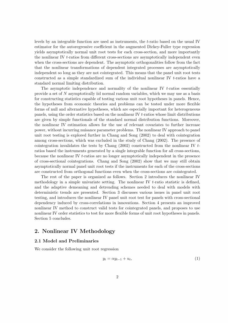
We consider the following unit root regression

yt = αyt−1 + ut, (1)

2

for t = 1, . . . , T . We are interested in testing the null of a unit root, α = 1, againstthe stationarity alternative, |α| < 1. The initial value y0 does not affect our subsequentasymptotic analysis as long as they are stochastically bounded, and therefore we set it atzero for expositional brevity. The errors (ut) in the model (1) are serially correlated andspecified as an AR(p) process given by

α(L)ut = εt (2)

where L is the usual lag operator and α(z) = 1−∑p

k=1 αkzk. We assume

Assumption 2.1 α(z) 6= 0 for all |z| ≤ 1.

Assumption 2.2 (εt) is an iid (0, σ2) sequence of random variables with E|εt|` < ∞for some ` > 4, and its distribution is absolutely continuous with respect to the Lebesguemeasure and has characteristic function ϕ such that limλ→∞ λrϕ(λ) = 0 for some r > 0.

Define a stochastic processes UT for (εt) as

UT (r) = T−1/2[Tr]∑t=1

εt

on [0, 1], where [s] denotes the largest integer not exceeding s. The process UT (r) takesvalues in the space of cadlag functions on [0, 1]. Under Assumption 2.2, an invarianceprinciple holds for UT , viz.,

UT →d U (3)

as T →∞, where U is Brownian motion withvariance σ2. It is also convenient to defineBT (r) from (ut), similarly as UT (r). Let α(1) = 1 −

∑pk=1 αk and π(1) = 1/α(1). Then

we have BT (r) = T−1/2∑[Tr]t=1 ut →d B(r) where B = π(1)U , as shown in Phillips and Solo

(1992). This implies that the process (yt) when scaled by T−1/2 behaves asymptotically asthe Brownian motion B under the null α = 1 of unit root.

Our limit theory involves the two-parameter stochastic process called local time of Brow-nian motion.2 We denote by L the (scaled) local time of U , which is defined by

L(t, s) = limε→0

12ε

∫ t

01{|U(r)− s| < ε} dr. (4)

The local time L is therefore the time that the Brownian motion U spends in the immediateneighborhood of s, up to time t, measured in chronological units. Then we may have animportant relationship ∫ t

0G(U(r)) dr =

∫ ∞−∞

G(s)L(t, s) ds

which we refer to as the occupation time formula. The conditions in Assumption 2.2 arerequired to obtain the convergence and invariance of the sample local time, as well asthose of the sample Brownian motion, for the asymptotics of integrable transformations ofintegrated time series.

2The reader is referred to Chung and Williams (1990) and the references cited in Park and Phillips (1999,2001) for the concept of local time and its use in the asymptotics for nonlinear models with integrated timeseries.

3

2.2 IV Estimation and Its Limit Theories

Taking the serial correlations in the error (ut) specified in (2) into the model (1) gives

yt = αyt−1 +p∑

k=1

αk4yt−k + εt (5)

where 4 is the difference operator, since 4yt = ut under the unit root null hypothesis.We consider the IV estimation of the augmented autoregression (5), using the followinginstruments

(F (yt−1),4yt−1, . . . ,4yt−p)′ (6)

where F is an integrable function. Notice that the instrument we use for the lagged levelyt−1 is an integrable transformation of itself, i.e., F (yt−1). For the lagged differences(4yt−1, . . . ,4yt−p), we use the variables themselves as the instruments. The transformationF is called instrument generating function (IGF) and assumed to satisfy

Assumption 2.3 Let F be integrable and satisfy∫ ∞−∞

xF (x)dx 6= 0.

The condition given in Assumption 2.3 requires that the instrument F (yt−1) is correlatedwith the regressor yt−1 that it is instrumenting for. It is shown for simple random walkmodels in Phillips, Park and Chang (1999) that IV estimators become inconsistent when theinstrument is generated by a regularly integrable function F such that

∫∞−∞ xF (x) dx = 0. It

is analogous to the non-orthogonality (between the instruments and regressors) requirementfor the validity of IV estimation in standard stationary regressions. In our nonstationary IVestimation, where an integrable function of an integrated regressor is used as the instrument,such instrument failure occurs when the instrument generating function is orthogonal to theregression function.

Define xt = (4yt−1, . . . ,4yt−p)′, and let y, y` and X be the observations on yt, yt−1

and xt, respectively. Using this notation, we write the regression (5) in matrix form as

y = y`α + Xβ + ε = Y γ + ε

where β = (α1, . . . , αp)′, Y = (y`, X), and γ = (α, β′)′. Denote by wt the instrumentalvariables given in (6), and let W = (F (y`), X) be the matrix of observations on wt, whereF (y`) = (F (yp), . . . , F (yT−1))′. We consider the following estimator γ for γ:

γ =(

αβ

)= (W ′Y )−1W ′y =

(F (y`)′y` F (y`)′X

X ′y` X ′X

)−1 (F (y`)′yX ′y

)(7)

which is the usual IV estimator of γ using the instruments wt. The IV estimator α for theAR coefficient α corresponds to the first element of γ, and is given by

α− 1 = B−1T AT (8)

4

under the null, where

AT =T∑

t=1

F (yt−1)εt −T∑

t=1

F (yt−1)x′t

(T∑

t=1

xtx′t

)−1 T∑t=1

xtεt

BT =T∑

t=1

F (yt−1)yt−1 −T∑

t=1

F (yt−1)x′t

(T∑

t=1

xtx′t

)−1 T∑t=1

xtyt−1

The variance of AT is given byσ2ECT

under Assumption 2.2, where

CT =T∑

t=1

F 2(yt−1)−T∑

t=1

F (yt−1)x′t

(T∑

t=1

xtx′t

)−1 T∑t=1

xtF (yt−1).

For testing the unit root hypothesis α = 1, we construct the t-ratio statistic from thenonlinear IV estimator α defined in (8) as

τ =α− 1s(α)

(9)

where s(α) is the standard error of the IV estimator α given by

s2(α) = σ2B−2T CT (10)

The σ2 is the usual variance estimator given by T−1∑Tt=1 ε2

t , where εt is the fitted residualfrom the augmented regression (5), i.e., εt = yt − αyt−1 − x′tβ. It is natural in our contextto use the IV estimate (α, β) given in (7) to get the fitted residual εt. However, we mayobviously use any other estimator of (α, β) as long as it yields a consistent estimate for theresidual error variance. The nonlinear IV t-ratio τ reduces to τ = σ−1AT C

−1/2T , due to (8),

(9) and (10).The following lemma presents the asymptotics for the sample product moments appear-

ing in the definition of τ .

Lemma 2.4 Under Assumptions 2.1, 2.2 and 2.3, we have

(a) T−1/4T∑

t=1

F (yt−1) εt →d MN(

0, σ2α(1)L(1, 0)∫ ∞−∞

F 2(s)ds

)(b) T−1/2

T∑t=1

F 2(yt−1) →d α(1)L(1, 0)∫ ∞−∞

F 2(s)ds

(c) T−3/4Ti∑

t=1

F (yt−1)4yt−k →p 0, for k = 1, . . . , p,

as T →∞.

Parts (a) and (b) can easily be obtained as in Park and Phillips (1999, 2001), using therecent extension made by Park (2003a).3 Part (c) is shown in Chang (2002).

3Park and Phillips (1999, 2001) impose piecewise higher-order Lipschitz conditions on F to derive theasymptotics here. Such conditions, however, are shown to be unnecessary in Park (2003a).

5

The result in part (a) shows that the covariance asymptotics of the integrable F yieldsa mixed normal limiting distribution with a mixing variate depending upon the local timeL of the limit Brownian motion U , as well as the integral of the square of the instrumentgenerating function F . It is indeed an intriguing result, which will lead to the normal limittheory for the nonlinear IV t-ratio. It is very useful to note

T−1/4T∑

t=1

F (yt−1)εt ≈d4√

T

∫ 1

0F (√

TB(r))dU(r)

T−1/2T∑

t=1

F 2(yt−1) ≈d

√T

∫ 1

0F 2(

√TB(r))dr

from which we may easily deduce the results in parts (a) and (b) using the theory ofcontinuous martingales and the relationship B = π(1)U with π(1) = 1/α(1). The reader isreferred to Park (2003b) for a heuristic of the results in parts (a) and (b) along this line.

The result in part (c) implies that the lagged differences 4yt−k, k = 1, . . . , p, and thenonlinear instrument F (yt−1) are asymptotically independent. This in turn implies that thepresence of the stationary lagged differences in our base regression (5) does not affect thelimit theory of the nonlinear IV estimator for the coefficient on the lagged level, which isan integrated process under the null. The rate T 3/4 at which the sample moment vanishesis obtained in Chang, Park and Phillips (2001). The asymptotic orthogonalities we havehere are analogous to the familiar asymptotic orthogonalities between the stationary andintegrated regressors we have seen in the usual cointegrating regressions, shown earlier inPark and Phillips (1988).

The limit null distribution of the IV t-ratio statistic τ now follows readily from theresults in Lemma 2.4, as in Phillips, Park and Chang (1999) and Chang (2002).

Theorem 2.5 Under Assumption 2.1, 2.2 and 2.3, we have

τ →d N(0, 1)

as T →∞.

The limiting distribution of τ for testing α = 1 is standard normal if a regularly integrablefunction is used to generate the instrument. The limit theory here is fundamentally differentfrom the asymptotics for the usual linear unit root tests such as those by Phillips (1987)and Phillips and Perron (1988). The use of nonlinear IV is essential for our Gaussian limittheory which is obtained from the local time asymptotics and mixed normality result givenin Lemma 2.4.

The nonlinear IV t-ratio statistic is a consistent test for testing the null of unit root. Tosee this, consider the limit behavior of the IV t-ratio τ given in (9) under the alternative ofstationarity, i.e., α = α0 < 1. We may express τ as

τ = τ(α0) +√

T (α0 − 1)√T s(α)

(11)

whereτ(α0) =

α− α0

s(α)(12)

6

which is the IV t-ratio for testing α = α0 < 1. Under the alternative, we may expect thatτ(α0) →d N(0, 1) if the usual mixing conditions for (yt) are assumed to hold. Moreover, if welet B0 = plimT→∞T−1BT and C0 = plimT→∞T−1CT exist under suitable mixing conditionsfor (yt), then the second term in the right hand side of equation (11) diverges to −∞ at therate of

√T under the alternative of stationarity. This is because

√T (α0 − 1) → −∞ and√

T s(α) →p ν, as T →∞, where ν2 = σ2B−20 C0 > 0. Hence, under the alternative

τ →p −∞

at√

T -rate, implying that the IV t-ratio τ is√

T -consistent, just as in the case of the usualOLS-based t-type unit root tests such as the augmented Dickey-Fuller test.

We note that the IV t-ratios constructed from integrable IGFs are asymptotically nor-mal, for all |α| ≤ 1, which makes a drastic contrast with the limit theory of the standardt-statistic based on the ordinary least squares estimator. The continuity of the limit distri-bution of the t-ratio in (12) across all values of α including the unity, in particular, allowsus to construct the confidence intervals for α from the nonlinear IV estimator α given in(8). We may construct 100 (1− λ) % asymptotic confidence interval for α as[

α− zλ/2 s(α), α + zλ/2 s(α)]

where zλ/2 is the (1 − λ/2)-percentile from the standard normal distribution. This is an-other important advantage of using the nonlinear IV method. The OLS-based standardt-ratio, such as ADF test, has non-Gaussian limiting null distribution called Dickey-Fullerdistribution. The DF distribution is tabulated in Fuller (1996) and known to be asymmetricand skewed to the left, rendering it impossible to construct an confidence interval which isvalid for all |α| ≤ 1 from the standard OLS based t-ratios.

2.3 IV Estimation for Models with Deterministic Trends

The models with deterministic components can be analyzed similarly as in the previoussection, if properly demeaned or detrended data are used. A proper demeaning or detrendingscheme required here must be able to successfully remove the nonzero mean or time trend,while maintaining the orthogonality of the demeaned or detrended series with the errorterm, which is essential in retaining the martingale property of the error and ultimately theGaussian limit theory of the covariance asymptotics for the nonlinear instrument. To meetthe needs described above, Chang (2002) devises the adaptive demeaning and detrending,which we introduce below.

For a time series (zt) with a nonzero mean given by

zt = µ + yt (13)

where the stochastic component (yt) is generated as in (1), we may test for a unit root in(yt) from the regression

yµt = αyµ

t−1 +p∑

k=1

αk4yµt−k + εt (14)

7

where yµt and yµ

t−1 are, respectively, the adaptively demeaned series of zt and zt−1 that aredefined as

yµt = zt −

1t− 1

t−1∑k=1

zk

yµt−1 = zt−1 −

1t− 1

t−1∑k=1

zk

4yµt−k = 4zt−k, k = 1, . . . , p.

The term (t−1)−1∑t−1k=1 zk appearing in the definitions above is the least squares estimator

of µ obtained from the preliminary regression

zk = µ + yk, for k = 1, . . . , t− 1.

We note that the mean µ is estimated from the model (13) using the observations up to time(t−1) only, rather than using the full sample. This leads to the demeaning based on thepartial sum of the data up to (t−1), and for this reason the above demeaning scheme is calledadaptive. Notice that even for the t-th observation zt, we use (t−1)-adaptive demeaningto maintain the martingale property. The lagged differences 4zt−k, k = 1, . . . , p, need nofurther demeaning, since the differencing has already removed the mean.

We may then construct the nonlinear IV t-ratio τµ to test for unit root in (yt) based onthe nonlinear IV estimator for α from the regression (14), just as in (9). The adaptivelydemeaned lagged level yµ

t−1 is orthogonal to the error εt, which ensures the predictability ofthe nonlinear instrument F (yµ

t−1), thereby retaining the martingale property of the error.Consequently, the sample moment T−1/4∑T

t=1 F (yµt−1)εt has mixed normal limit theory, as

in the models with no deterministic trends given in Lemma 2.4 (a), leading to the normaldistribution theory for the IV t-ratio τµ for the models with nonzero mean.

We may also test for a unit root in the stochastic component of the time series withlinear time trend using the nonlinear IV t-ratio τ τ constructed in the similar manner usingadaptively detrended data. For a time series with a linear time trend given by

zt = µ + δt + yt (15)

where (yt) is generated as in (1), we may use the following regression as the basis for testingunit root in the stochastic component (yt):

yτt = αyτ

t−1 +p∑

k=1

αk4yτt−k + et (16)

where yτt , yτ

t−1 and4yτt−k are adaptively detrended series of zt, zt−1 and4zt−k, k = 1, . . . , p,

given as

yτt = zt +

2t− 1

t−1∑k=1

zk −6

t(t− 1)

t−1∑k=1

kzk −1T

zT

8

yτt−1 = zt−1 +

2t− 1

t−1∑k=1

zk −6

t(t− 1)

t−1∑k=1

kzk

4yτt−k = 4zt−k −

1T i

zT , k = 1, . . . , p,

and (et) are the regression errors. The variables zt and zt−1 are detrended using the leastsquares estimators of the drift and trend coefficients, µ and δ, from the model (15) usingagain the observations up to time (t−1) only, viz.,

zk = µ + δk + yik, for k = 1, . . . , t− 1.

The term T−1zT apprearing in the definitions of yτt and 4yτ

t−k, k = 1, . . . , p, is the grandsample mean of 4zt, i.e., T−1∑T

k=14zk. The grand sample mean is needed for yτt to

eliminate the remaining the drift term of zt + 2(t− 1)−1∑t−1k=1 zk − 6(t(t− 1))−1∑t−1

k=1 kzk,and for 4yτ

t−k to remove the nonzero mean of 4zt−k, for k = 1, . . . , p.The nonlinear IV t-ratio τ τ is then defined as in (9) from the nonlinear IV estimator for

α from the regression (16) with the detrended data. The adaptive detrending of the datagiven above also preserves the predictability of the instrument F (yτ

t−1), and the martingaleproperty of the error et is also retained in this case, as shown in Chang (2002). Theseensure the mixed normal limit theory of the the sample moment T−1/4∑T

t=1 F (yτt−1)et

and the normal limit theory for the IV t-ratio τ τ . For the actual derivation of the limittheories for the statistics τµ and τ τ , we need to characterize the limit processes of theadaptively demeaned and detrended series, (yµ

t ) and (yτt ). When scaled by T−1/2, (yµ

t ) and(yτ

t ) converge in distribution to the constant π(1) multiple of the adaptively demeandedBrownian motion Uµ and the adaptively detrended Brownian motion U τ , resectively. Moreexplicitly, the adaptively demeaned Brownian is defined as

Uµ(r) = U(r)− 1r

∫ r

0U(s)ds

and similarly the adaptively detrended Brownian motion as

U τ (r) = U(r) +2r

∫ r

0U(s)ds− 6

r2

∫ r

0sU(s)ds

If we let Uµ(0) = 0 and U τ (0) = 0, then both processes have well defined continuousversions on [0,∞), as shown in Chang (2002).

The asymptotic results given in Lemma 2.4 extend easily to the models with nonzeromeans and deterministic trends if we replace the lagged level yt−1 with the lagged detrendedseries yµ

t−1 and yτt−1. They are indeed given similarly with the local times Lµ and Lτ of

the adaptively demeaned and detrended Brownian motions Uµ and U τ in the place of thelocal time L of the Brownian motion U . Then the limit theories for the nonlinear IV t-ratiostatistics τµ and τ τ for the models with nonzero means and deterministic trends followimmediately, as shown in Chang (2002), and are given in

Corollary 2.6 Under Assumption 2.1, 2.2 and 2.3, we have

τµ, τ τ →d N(0, 1)

9

as T →∞.

The standard normal limit theory of the nonlinear IV t-ratio for the models with no de-terministic trends given in Theorem 2.5, therefore, continues to hold for the models withnonzero mean and linear time trend.

3. Panel Unit Root Tests

3.1 Issues in Panel Unit Root Testing

A number of unit root tests for panel data have been developed in the recent literature,including most notably those by Levin, Lin and Chu (2002) and Im, Pesaran and Shin(1997). However, they all have some important drawbacks and limitations. The test pro-posed by Levin, Lin and Chu (2002) is applicable only for homogeneous panels, where theAR coefficients for unit roots are in particular assumed to be the same across cross-sections.Their tests are based on the pooled OLS estimator for the unit root AR coefficient, andtherefore, cannot be used for heterogeneous panels with different individual unit root ARcoefficients. In addition, they assume cross-sectional independence. Im, Pesaran and Shin(1997) allow for the heterogeneous panels and propose the unit root tests which are basedon the average of the individual unit root tests, t-statistics and LM statistics, computedfrom each individual unit. The validity of their tests, however, also require cross-sectionalindependence. Needless to say, the cross-sectional independence and homogeneity are quiterestrictive assumptions for most of the economic panel data we encounter.

Chang (2002) explores the nonlinear IV methodology introduced in the previous sec-tion to solve the inferential difficulties in the panel unit root testing which arise from theinstrinsic heterogeneities and dependencies of panel models. For each cross-section, the t-statistic for testing the unit root is constructed from the IV estimator of the autoregressivecoefficient obtained from using an integrable transformation of the lagged level as instru-ment. As expected from our earlier results, each individual nonlinear IV t-ratio statisticconstructed as such has standard normal limit null distribution. What is more important,however, is that the individual IV t-ratio statistics are asymptotically independent evenacross dependent cross-sectional units. This is indeed an intriguing result and follows fromthe asymptotic orthogonality results established in Chang, Park and Phillips (2001) for thenonlinear transformations of integrated processes by an integrable function.

The most important implication of the asymptotic normality and orthogonalities of theindividual nonlinear IV t-ratios is that we now have a set of N asymptotically independentstandard normal random variables to construct the unit root test for panels with N cross-sections. Of course, a simple average, defined as a standardized sum, of the individual IVt-ratios is a valid statistic for testing joint unit root null hypothesis for the entire panel.Chang (2002) shows that such a normalized sum of the individual IV t-ratios also hasstandard normal limit distribution, as long as the number of observations in each individualunit is large and the panel is asymptotically balanced in a weak sense. The standard limittheory is thus obtained without having to require the sequential asymptotics,4 upon which

4The usual sequential asymptotics is carried out by first passing T to infinity with N fixed, and subse-

10

most of the available asymptotic theories for panel unit root models heavily rely. As aresult, we may allow the number of cross-sectional units N to be arbitrarily small as well aslarge. The asymptotics developed here are T -asymptotics, and we assume that N is fixedthroughout the paper.

However, there remains three important issues yet to be addressed. First, the presenceof cointegration across cross-sectional units has never been allowed. It appears that thereis a high potential for such possibilities in many panels of practical interests. Yet noneof the existing tests, including the nonlinear IV panel unit root test by Chang (2002)discussed above, is applicable for such panels. Second, there is an issue of using covariates.As demonstrated by Hansen (1995) and Chang, Sickles and Song (2001), the inclusion ofcovariates can dramatically increase the power of the tests. Nevertheless, the pontentialhas never been investigated in the context of panels. Third, the issue of formulating thepanel unit root hypothesis remains largely unresolved. We often need to consider the nulland alternative hypotheses that some, not all, of the cross-sectional units have unit roots.Though none has seriously considered such hypotheses, they seem to be more relevant formany practical applications. The nonlinear IV methodology can be extended to resolve allthese issues, as shown in Chang and Song (2002).

The improved IV methodology introduced in Chang and Song (2002) is based on theADF regression further augmented with stationary covariates, and uses the instrumentsgenerated by a set of orthogonal functions. The use of orthogonal instrument generat-ing functions for each cross-section is crucial for retaining the Gaussian limit theory andasymptotic orthogonalities of the nonlinear IV t-ratios in cointegrated panels. With theseproperties, the nonlinear IV t-ratios computed from N cross-sections continue to serve asa basis of N asymptotically iid standard normal random variables, which can be used toconstruct various unit root tests. In particular, we may use the order statistics, minimumor maximum, of the nonlinear IV t-ratios to test for or againt the existence of the unitroots in not all, but only in a fraction of the cross-sectional units. The limit distributionsof the order statistics computed from the nonlinear IV t-ratios are nuisance parameter freeand given by simple functionals of the standard normal distribution functions, as shown inChang and Song (2002). This implies in particular that the critical values of the tests canbe obtained from the standard normal table.

The nonlinear IV based panel unit root testing is indeed very general and applicablefor a wide class of panel models. The nonlinear IV methodology, more specifically theasymptotic independence and normality of the nonlinear IV t-ratios, allows us to derivesimple Gaussian limit theories for the panel unit root tests in panels with cross-sectionaldependency at all levels. We may allow for cross-correlations of the innovations and/orcross-sectional dynamics in the short-run, and also for the comovements of the individualstochastic trends in the long-run. The nonlinear IV approach also allows us to formulatehypotheses in a much sharper form, which in turn makes it possible to test for and againstthe existence of unit roots in a sub-group of the cross-sections. Such general results arenot entertained in other existing testing procedures, since their results require either cross-sectional independence or rely on a specific form of cross-sectional correlation structure,

quently let N go to infinity, usually under cross-sectional independence.

11

which may have a limited applicability in practice.In what follows we first present the nonlinear IV unit root test for the dependent panels

with no cointegration among cross-sections in Section 3.2, and subsequently in Section 4.1introduce the improved IV methodology for cointegrated panels. In Section 4.2 the issueof properly formulating unit root hypotheses in panels is then discussed, and nonlinear IVorder statistics are presented as vehicles to conduct testing for more flexibly formulatedhypotheses.

3.2 Nonlinear IV Panel Unit Root Tests

We consider a panel unit root model given by

yit = αiyi,t−1 + uit, i = 1, . . . , N ; t = 1, . . . , T . (17)

As usual, the index i denotes individual cross-sectional units, such as individuals, house-holds, industries or countries, and the index t denotes time periods. The cross-sectionaldimension N is not restricted and allowed to take large or small values. For expositionalsimplicity, the cross-sections are assumed to have the same T number of observations; how-ever, the results here easily extend to unbalanced panels, as we discuss later in the section.The error terms uit are allowed to have serial correlations, which we specify by an AR pro-cess of order pi, i.e., αi(L)uit = εit, where αi(z) = 1 −

∑pik=1 αikz

k, for i = 1, . . . , N . Notethat we let αi(z) and pi vary across i, thereby allowing heterogeneity in individual short-run dynamic structures. The cross-sections are allowed to be dependent via cross-sectionaldependency of the innovations εit, i = 1, . . . , N , that generate the errors uit. To be moreexplicit about the cross-sectional dependency we allow here, define (εt)T

t=1 by

εt = (ε1t, . . . , εNt)′ (18)

We allow the N -dimensional innovation process (εt) to have covariance matrix Σ, which isunrestricted except for being positive definite.

We are interested in testing whether the series (yit) generated as in (17) has a unit rootin all cross-sections i = 1, . . . , N , against the alternative that (yit) are stationary in somecross-section i. The null hypothesis is therefore formulated as H0 : αi = 1 for all i, andtested against the stationarity alternative H1 : |αi| < 1 for some i. The test statistic wefirst consider for testing the panel unit root hypothesis is a simple average of the individualnonlinear IV t-ratio statistics for testing the unity of the AR coefficient computed fromeach cross-sectional unit. Under the AR(pi) specification of the error uit, the model (17) iswritten as

yit = αiyi,t−1 +pi∑

k=1

αik4yi,t−k + εit, i = 1, . . . , N ; t = 1, . . . , T (19)

which is identical, at each cross-section level, to the regression (5) used in the previoussection to derive the univariate nonlinear IV t-ratio given in (9). For each cross-section i,

12

we therefore instrument the lagged level yi,t−1 using an integrable transformation of itselfF (yi,t−1), and accordingly define the nonlinear IV t-ratio τi for testing αi = 1 as

τi =αi − 1s(αi)

where αi and s(αi) are, respectively, the nonlinear IV estimator of αi and its standarderror, defined as in (8) and (10). The limit theories for each individual IV t-ratio τi followexactly in the same manner as for the univariate nonlinear IV t-ratio given in Lemma 2.4and Theorem 2.5, under the same set of conditions modified for our panel setting here.Let | · | denote the Euclidean norm: for a vector x = (xi), |x|2 =

∑i x

2i , and for a matrix

A = (aij), |A| =∑

i,j a2ij . We assume

Assumption 3.1 For i = 1, . . . , N , αi(z) 6= 0 for all |z| ≤ 1.

Assumption 3.2 (εt) is an iid (0,Σ) sequence of random vectors with E|εt|` < ∞ forsome ` > 4, and its distribution is absolutely continuous with respect to Lebesgue measureand has characteristic function ϕ such that limλ→∞ |λ|rϕ(λ) = 0, for some r > 0.

Under Assumption 3.2, an invariance principle holds for the partial sum process UT ofthe N -vector innovations (εt), i.e., UT →d U as T →∞, where U = (U1, . . . , UN)′ is anN -dimensional vector Brownian motion with covariance matrix Σ. It is also convenientto define BT (r) from ut = (u1t, . . . , uNt)′, similarly as UT (r). Let αi(1) = 1 −

∑pik=1 αik

and πi(1) = 1/αi(1). Then under Assumptions 3.1 and 3.2 we have BT →d B, whereB = (B1, . . . , BN)′ and Bi = πi(1)Ui for i = 1, . . . , N . The local times that appear in ourlimit theory are Li that are (scaled) local time of Ui, for i = 1, . . . , N . As shown in Chang(2002), we have

Theorem 3.3 Under Assumptions 2.3, 3.1 and 3.2, we have

τi →d N(0, 1)

as T →∞ for all i = 1, . . . , N , and

τi, τj ∼ asymptotically independent

for all i 6= j = 1, . . . , N .

The standard normal limit theory of the univariate nonlinear IV t-ratio τ given in Theorem2.5 continues to apply for each individual IV t-ratio τi for i = 1, . . . , N . Moreover, thenonlinear IV t-ratios from different cross-sections are asymptotically independent even undercross-sectional dependency. The asymptotic orthogonalities of the nonlinear IV t-ratios playa crucial role in developing our panel unit root test, since these, along with the Gaussianityof the individual IV t-ratios, provide a basis of N asymptotically iid normal random variatesfor us to work with.

Before we proceed to define our panel unit root test, we provide some heuristics tounderstand the important asymptotic orthogonalities. We have the following distributional

13

equivalences in the limit for the sample moments determining the limit theories of the IVt-ratios τi and τj from the cross-sections i and j

T−1/4T∑

t=1

F (yi,t−1)εit ≈d4√

T

∫ 1

0F (√

TBi(r))dUi(r)

T−1/4T∑

t=1

F (yj,t−1)εjt ≈d4√

T

∫ 1

0F (√

TBj(r))dUj(r)

It is well known that the two right hand side stochastic processes become asymptoticallyindependent if their quadratic covariation

σij

√T

∫ 1

0F (√

TBi(r))F (√

TBj(r))dr (20)

converges a.s. to zero, where σij denotes the covariance between Ui and Uj . The order of theintegral

∫ 10 F (

√TBi(r))F (

√TBj(r))dr in the above equation is known to be Op(T−1 log(T ))

a.s., due to Kasahara and Kotani (1979), which in turn implies that the quadratic covariation(20) vanishes almost surely, regardless of the value of σij . The reasons why the integral isof such a small order are two-fold. The first is that the instrument generating function Fis an integrable function which assigns a non-trivial value only when the argument takes asmall value; and the second is that each of the arguments

√TBi and

√TBj takes a large

value with increasing probability as T grows, due to the stochastic trends in the Brownianmotions Bi and Bj . As a result, the product F (

√TBi)F (

√TBj) takes a non-trivial value

only with a small probability, making the above integral of such a small order.Notice that Ui and Uj are the limit Brownian motions of the innovations (εit) and (εjt)

generating the (yit) and (yjt). The above result therefore shows that the nonlinear instru-ments F (yi,t−1) and F (yj,t−1) from different cross-sectional units i and j are asymptoticallyuncorrelated, even when the variables (yit) and (yjt) generating the instruments are cor-related. This then implies that the individual IV t-ratio statistics τi and τj constructedfrom the nonlinear instruments, F (yi,t−1) and F (yj,t−1), are asymptotically independent.Hence, we may naturally consider an average of such asymptotically normal and indepen-dent nonlinear IV t-ratios to test for the joint unit root null hypothesis H0 : αi = 1 for alli = 1, . . . , N . The test is defined as

S =1√N

N∑i=1

τi (21)

and the limit theory for S follows immediately from Theorem 3.3 as

Theorem 3.4 We haveS →d N(0, 1)

as T →∞ under Assumptions 2.3, 3.1 and 3.2.

Our limit theories derived here for the balanced panels continue to hold for the unbal-anced panels, where each cross-section i may have a different number Ti of observations,

14

as shown in Chang (2002). To deal with the unbalanced nature of the data, we only needto ensure that the panel is asymptotically balanced in a weak sense. Specifically, it is re-quired that Ti → ∞ for all i, and T

−3/4min T

1/4max log(Tmax) → 0, where Tmin and Tmax denote,

repectively, the minimum and the maximum of Ti, i = 1, . . . , N . Note that our limit the-ory is derived using T -asymptotics only, and the factor N−1/2 in the definition of the teststatistic S in (21) is used just as a normalization factor, since S is based on the sum ofN independent random variables. This implies the dimension of the cross-sectional unitsN may take any value, small as well as large. Our results also extend to the panels withheterogeneous deterministic components, such as individual fixed effects and linear timetrends. The asymptotic results established here for the models without deterministic com-ponents continue to hold for those with nonzero means and linear trends, if the nonlinear IVestimation in each cross-section is based on the properly detrended data, using the adaptivedemeaning or detrending scheme introduced in Section 2.3. The standard normal theoryfor our nonlinear IV panel unit root test constructed from the adaptively detrended data,therefore, continues to hold for the panels with heterogeneous fixed effects and time trends.

The normal limit theory is also obtained for the existing panel unit root tests, suchas the pooled OLS test by Levin, Lin and Chu (2002) and the group mean t-bar statisticby Im, Pesaran and Shin (1997); however, their theory holds only under cross-sectionalindependence, and is obtained only through sequential asymptotics. More recently, sev-eral authors have made serious attempt to allow for cross-sectional dependencies. Chang(1999) allows for dependencies of unrestricted form, but her bootstrap procedure requiresthe dimension of time series T to be substantially larger than that of the cross-section N ,which is restrictive for many practical applications. On the other hand, the procedures byChoi (2001), Phillips and Sul (2001) and Moon and Perron (2001) allow for a specific formof cross-sectional correlation structures, which may find only little justification in practicalapplications. In constrast, here we achieve the standard limit theory from the Gaussianityand independence of the limit distributions of the individual IV t-ratios, without having toassume independence across cross-sectional units, or relying on specific correlation struc-tures. We can now do simple inference for panel unit root testing based on the critical valuesfrom the standard normal table in dependent panels driven by cross-correlated innovationsand with various heterogeneities.

4. Extensions and Generalizations

4.1 Cointegrated Panels with Covariates

Our nonlinear IV approach can be extended to allow for the presence of cross-sectionalcointegration and the use of relevant stationary covariates. We now let yt = (y1t, . . . , yNt)′

and assume that there are N −M cointegrating relationships in the unit root process (yt),which are represented by the cointegrating vectors (cj), j = 1, . . . , N − M . The usualvector autoregression and error correction representation allows us to specify the short-run

15

dynamics of (yt) as

4yit =N∑

j=1

Pij∑k=1

aij4yj,t−k +N−M∑j=1

bijc′jyt−1 + εit (22)

for each cross-sectional unit, i = 1, . . . , N .Our unit root tests at individual levels will be based on the regression

yit = αiyi,t−1 +Pi∑

k=1

αik4yi,t−k +Qi∑

k=1

β′ikwi,t−k + εit (23)

for i = 1, . . . , N , where we interpret (wit) as the covariates added to the augmented DFregression for the i-th cross-sectional unit. It is important to note that the vector autoregres-sion and error correction formulation of the cointegrated unit root panels in (22) suggeststhat we use such covariates. Under the null, we may obviously rewrite (1) and (22) as (23)with the covariates which may include several lagged differences of other cross-sections andlinear combinations of lagged levels of all cross-sections. Indeed, in many panels of interest,we naturally expect to have inter-related short-run dynamics, which would make it neces-sary to include the dynamics of other cross-sections to properly model the dynamics in anindividual unit. In the presence of cointegration, we also need to incorporate the long-runtrends of other cross-sectional units, since the stochastic trends of other cross-sectional unitswould interfere with the short-run dynamics in an individual unit through the error cor-rection mechanism. Hence, the potential covariates for unit root testing in a cointegratedpanel include the lagged differences of other cross-sections to account for interactions inshort-run dynamics and the linear combinations of cross-sectional levels in the presence ofcointegration. Other stationary covariates may also be included to account for idiosyncraticcharacteristics of cross-sectional units.

The idea of using stationary covariates in the unit root regression was first entertainedby Hansen (1995) in a univariate context, and pursued further by Chang, Sickles and Song(2001) using a bootstrap method. Both papers clearly demonstrate that the use of mean-ingful covariates offers a great potential in power gains for the test of a unit root. In light ofthe fact that one of the main motivations to use panels to test for unit roots is to increasethe power, we have indeed overlooked this important opportunity in panel unit root testing.Choosing proper covariates can be a difficult issue in univariate applications, and the limitdistribution of the standard covariates augmented ADF test by Hansen (1995) involves anuisance parameter. In a panel context, however, there are many natural candidates forcovariates, such as those listed above. Moreover, the nonlinear instruments are asymptot-ically orthogonal to the stationary covariates, as shown in Chang and Song (2002), andtherefore the inclusion of the stationary covariates does not incur the nuisance parameterproblem for our nonlinear IV tests.

Denote as before by U = (U1, . . . , UN)′ the limit of the partial sum process constructedfrom the N -vector innovations εt = (ε1t, . . . , εNt)′, which is assumed to satisfy the conditionsin Assumption 2.2, and define B = (B1, . . . , BN)′ to be the corresponding limit Brownianmotion for ut = (u1t, . . . , uN)′. As is well known, the presence of cointegration in (yt) implies

16

that the vector Brownian motion B is degenerate, i.e., some of the individual limit Brownianmotions Bi, i = 1, . . . , N , are linearly dependent. This has important consequences for ourasymptotic analyses. Most importantly, the asymptotic orthogonalities of the nonlinear IVt-ratios no longer hold. This is because the quadratic covariation given in (20) no longervanishes in the limit. To see this, suppose Bi = Bj for some i and j. Then the quadraticcovariation becomes

σij

√T

∫ 1

0F (√

TBi(r))F (√

TBi(r))dr = σij

√T

∫ 1

0F 2(

√TBi(r))dr = Op(1), a.s.

since the integral∫ 10 F 2(

√TBi(r))dr is now of order Op(T−1/2), which is higher than the

order for the case with no cointegration, given below Theorem 3.3. This is because the inte-gral now involves an integrable function of only one Brownian motion, viz., F 2(

√TBi),

which takes a nontrivial value with much larger probability compared to the productF (√

TBi)F (√

TBj).The presence of cointegration can be dealt with if we use an orthogonal set of functions

as IGFs. This idea is exploited in Chang and Song (2002). It is indeed easy to see that thequadratic covariation given above may vanish in the limit if we use orthogonal functionsFi and Fj to generate the instruments for cross-sections i and j. As shown in, e.g., Park(2003b),

√T

∫ 1

0Fi(√

TBi(r))Fj(√

TBi(r))dr →a.s. 0

if Fi and Fj are orthogonal, and∫∞−∞ Fi(x)Fj(x) dx = 0.

The Hermite functions of odd orders k = 2i− 1, i = 1, . . . , N , for instance, can be usedas a valid set of IGFs for the cointegrated panels. The Hermite function Gk of order k,k = 0, 1, 2, . . ., is defined as

Gk(x) = (2kk!√

π)−1/2Hk(x)e−x2/2

where Hk is the Hermite polynomial of order k given by

Hk(x) = (−1)kex2 dk

dxke−x2

It is well known that the class of Hermite functions introduced above forms an orthonormalbasis for L2(R), i.e., the Hilbert space of square integrable functions on R. We thus have∫ ∞

−∞Gj(x)Gk(x)dx = δjk

for all j and k, where δjk is the kronecker delta. Moreover, the odd order Hermite functionssatisfy the IGF validity conditions in Assumption 2.3.

The IV estimation for the regression (23) is straightforward, given our discussions here.To deal with the cross-sectional cointegration, we use the instrument Fi(yi,t−1) for the laggedlevel yi,t−1 for each cross-sectional unit i = 1, . . . , N , where (Fi) is a set of orthogonal IGFs.For the augmented regressors xit = (4yi,t−1, . . . ,4yi,t−Pi ;wi,t−1, . . . , wi,t−Qi)

′, we use the

17

variables themselves as the instruments. Hence the instruments (F (yi,t−1), x′it)′ are used

for the entire regressors (yi,t−1, x′it)′. As is well expected, our previous asymptotic results

apply also in this more general context. In particular, the limit theories in Theorems 3.3and 3.4 continue to hold for the IV t-ratios τi’s and also for the panel unit root statistic Sin the presence of cointegration and covariates, if constructed in the way suggested above.This is shown in Chang and Song (2002).

4.2 Formulations of Hypotheses and Order Statistics

We now turn to the problems of formulating unit root hypotheses in panels, which was con-sidered in Chang and Song (2002). For many practical applications, we are often interestedin testing for unit roots collectively for a group of cross-sectional units included in the givenpanel. In this case, we need to more precisely formulate both the null and the alternativehypotheses. In particular, we may want to test for and against the existence of unit rootsin not all, but only a fraction of cross-sectional units. Such formulations, however, seemmore relevant and appropriate for many interesting empirical applications, including testingfor purchasing power parity and growth convergence, among others. Here we lay out threesets of possible hypotheses in panel unit root testing and propose to use the order statisticsconstructed from the nonlinear IV t-ratios to effectively test for such hypotheses.

We consider

Hypotheses (A) H0 : αi = 1 for all i versus H1 : αi < 1 for all i

Hypotheses (B) H0 : αi = 1 for all i versus H1 : αi < 1 for some i

Hypotheses (C) H0 : αi = 1 for some i versus H1 : αi < 1 for all i

Hypotheses (A) and (B) share the same null hypothesis that a unit root is present in all in-dividual units. However, the null hypothesis competes with different alternative hypotheses.In Hypotheses (A), the null is tested against the alternative hypothesis that all individualunits are stationary, while in Hypothesis (B) it is tested against the alternative that thereare some stationary individual units. On the contrary, the null hypothesis in Hypotheses(C) holds as long as unit root exists in at least one individual unit, and is tested against thealternative hypothesis that all individual units are stationary. The alternative hypotheses inboth Hypotheses (B) and (C) are the negations of their respective null hypotheses. This is,however, not the case for Hypotheses (A). Hypotheses (C) has never been considered in theliterature. Note that the rejection of H0 in favor of H1 in Hypotheses (C) directly impliesthat all (yit)’s are stationary, and therefore, purchasing power parities or growth conver-gence hold if we let (yit)’s be real exchange rates or differences in growth rates respectively.No test, however, is available to deal with Hypotheses (C) appropriately.

For the tests for Hypotheses (A)–(C), we define

S =1√N

N∑i=1

τi

18

Smin = min1≤i≤N

τi

Smax = max1≤i≤N

τi

where τi is the nonlinear IV t-ratio for the i-th cross-sectional unit. The averaged statistic Sis comparable to other existing tests and proposed for the test of Hypotheses (A). Virtuallyall of the existing panel unit root tests effectively test for Hypotheses (A). Some recentwork, including Im, Pesaran and Shin (1997) and Chang (2002), formulate their null andalternative hypotheses as in Hypotheses (B). However, their use of average t-ratios can onlybe justified for the test of Hypotheses (A). The minimum statistic Smin is more appropriatefor the test of Hypotheses (B) than the tests based on the averages. The average statisticS may also be used to test for Hypotheses (B), but the test based on Smin would have morepower, especially when only a small fraction of cross-sectional units are stationary underthe alternative hypothesis. The maximum statistic Smax can be used to test Hypotheses(C). Obviously, the average statistic S cannot be used to test for Hypotheses (C), since itwould have incorrect size.

Let M be 0 ≤ M ≤ N , and assume αi = 1 for 1 ≤ i ≤ M , and set M = 0 if αi < 1 for all1 ≤ i ≤ N . It is easy to derive the asymptotic theories for the test statistics defined above.Recall that the nonlinear IV t-ratios for all individual cross-sections have standard normallimiting distributions, and are asymptotically orthogonal to each other. This leaves us a setof M random variates τi’s that are asymptotically independent and identically distributedas standard normal. To obtain the asymptotic critical values for the statistics S, Smin andSmax, we let Φ be the distribution function for the standard normal distribution, and let λbe the size of the tests. For a given size λ, we define xM (λ) (with x1(λ) = x(λ)) and yN (λ)by

Φ(xM (λ))M = λ, (1− Φ(yN (λ)))N = 1− λ

These provide the critical values of the statistics S, Smin and Smax for the tests of Hypotheses(A) – (C). The following table shows the tests and critical values that can be used to testeach of Hypotheses (A) – (C).

Hypotheses Test Statistics Critical Values

Hypotheses (A) S x(λ)

Hypotheses (B) S x(λ)Smin yN (λ)

Hypotheses (C) Smax x(λ)Smax xM (λ)

It is clear that

limT→∞

P{S ≤ x(λ)} = λ

19

limT→∞

P{Smin ≤ yN (λ)} = λ

if M = N . The tests using statistics S and Smin with critical values x(λ) and yN (λ),respectively, have the exact size λ asymptotically under the null hypotheses in Hypotheses(A) and (B).

Moreover, if 1 ≤ M ≤ N , then

limT→∞

P{Smax ≤ xM (λ)} = λ, limT→∞

P{Smax ≤ x(λ)} ≤ λ

The null hypothesis in Hypotheses (C) is composite, and the rejection probabilities of thetest Smax based on the critical value x(λ) may not be exactly λ even asymptotically. Thesize λ in this case is the maximum rejection probabilities that can be obtained under thenull hypothesis.

The above results imply that the nonlinear IV order statistics suggested here havelimit distributions which are nuisance parameter free and given by simple functions of thestandard normal distribution function. The critical values are thus easily derived from thoseof the standard normal distribution.

5. Conclusion

The paper takes the nonlinear IV approach to testing for unit roots in general panelswith dependency and heterogeneity. The nonlinear IV based tests have many desirableproperties. First, the tests permit both short and long-run cross-sectional dependencies ofthe most general form. The presence of cointegration, the inter-relatedness of short-rundynamics and the cross-correlations in the errors are all allowed. This is in sharp constrastwith other existing tests, which assume complete cross-sectional independence of the errors.Second, various heterogeneities are allowed. Heterogeneities in dynamics, individual fixedeffects and trends, and the number of individual time series observations are all permitted inour framework. Third, the tests are very flexible to accommodate the extensions in variousdirections. In particular, they enable us to use relevant stationary covariates without havingto run into nuisance parameter problems. For the standard approach, the use of covariatesyields limit distributions including nuisance parameters that are difficult to deal with. Theycan also be extended to test for cointegration, as will be reported in a later work. Finally,our nonlinear IV method makes it possible to formulate the panel unit root hypotheses inmore flexible and more precise forms, which can be tested by various order statistics. Withthe tests provided here, the empirical researchers will be able to investigate much moreprecisely and rigorously a wide variety of important economic issues regarding internationaland interstate comparisons and interactions including purchasing power parities and growthconvergences/divergences.

6. References

Baltagi, B.H. and C. Kao (2000). “Nonstationary panels, cointegration in panels anddynamic panels: A survey,” mimeographed, Department of Economics, Texas A& M

20

University.

Chang, Y. (1999). “Bootstrap unit root tests in panels with cross-sectional dependency,”forthcoming in Journal of Econometrics.

Chang, Y. (2002). “Nonlinear IV Unit Root Tests in Panels with Cross-Sectional Depen-dency,” Journal of Econometrics 110, 261-292.

Chang, Y. and W. Song (2002).“Panel Unit Root Tests in the Presence of Cross-SectionalDependency and Heterogeneity,” mimeographed, Department of Economics, Rice Uni-versity.

Chang, Y., J.Y. Park and P.C.B. Phillips (2001). “Nonlinear econometric models withcointegrated and deterministically trending regressors,” Econometrics Journal 4, 1-36.

Chang, Y., R.C. Sickles and W. Song (2001). “Bootstrapping unit root tests with covari-ates,” mimeographed, Department of Economics, Rice University.

Choi, I. (2001). “Unit root tests for cross-sectionally correlated panels,” mimeographed,Kukmin University.

Chung, K.L. and Williams, R.J. (1990). Introduction to Stochastic Integration, 2nd ed.Birkhauser, Boston.

Hansen, B.E. (1995). “Rethinking the univariate approach to unit root testing: Usingcovariates to increase power,” Econometric Theory 11, 1148-1171.

Im, K.S., M.H. Pesaran and Y. Shin (1997). “Testing for unit roots in heterogeneouspanels,” mimeographed.

Kasahara, Y. and S. Kotani (1979). “On limit processes for a class of additive functionalsof recurrent diffusion processes,” Z. Wahrscheinlichkeitstheorie verw. Gebiete 49, 133-153.

Levin, A., C.F. Lin and C.S. Chu (2002). “Unit root tests in panel data: Asymptotic andfinite sample properties,” Journal of Econometrics 108, 1-24.

Maddala, G.S. and S. Wu (1999). “A comparative study of unit root tests with panel dataand a new simple test: Evidence from simulations and bootstrap,” Oxford Bulletin ofEconomics and Statistics 61, 631-.

Moon, H.R. and B. Perron, (2001). “Testing for a unit root in panels with dynamicfactors,” mimeographed.

Park, J.Y. (2003a). “Strong approximations for nonlinear transformations of integratedtime series,” mimeographed, Department of Economics, Rice University.

Park, J.Y. (2003b). “Nonstationary nonlinearity: An outlook for new opportunities,”mimeographed, Deparment of Economics, Rice University.

21

Park, J.Y. and P.C.B. Phillips (1988). “Statistical Inference in Regressions with IntegratedProcesses: Part 1,” Econometric Theory 5, 468-498.

Park, J.Y. and P.C.B. Phillips (1999). “Asymptotics for nonlinear transformations ofintegrated time series,” Econometric Theory 15: 269-298.

Park, J.Y. and P.C.B. Phillips (2001). “Nonlinear regressions with integrated time series,”Econometrica 69, 1452-1498.

Phillips, P.C.B. (1987). “Time series regression with a unit root,” Econometrica 55, 277-301.

Phillips, P.C.B. and H.R. Moon (2000). “Nonstationary Panel Data Analysis: An Overviewof Some Recent Developments,” Econometric Reviews 19, 263-286.

Phillips, P.C.B., J.Y. Park and Y. Chang (1999). “Nonlinear instrumental variable esti-mation of an autoregression,” forthcoming in Journal of Econometrics.

Phillips, P.C.B and P. Perron (1988). “Testing for a unit root in time series regression,”Biometrika 75, 335-346.

Phillips, P.C.B. and V. Solo (1992). “Asymptotics for linear processes,” Annals of Statistics20, 971-1001.

Phillips, P.C.B. and D. Sul (2001). “Dynamic panel estimation and homogeneity testingunder cross section dependence,” mimeographed, University of Auckland.

22