Nonlinear equations and elliptic curves

NONLINEAR EQUATIONS AND ELLIPTIC CURVES

I. M. Krichever UDC 517.957+512.7

The main ideas of global "finite-zone integration" are presented, and a detailed analysis is given of applications of the technique developed to some problems based on the theory of elliptic functions. In the work the Peierls model is inte- grated as an important application of the algebrogeometric spectral theory of difference operators.

INTRODUCTION

During the last 10-15 years one of the most powerful tools in the investigation of nonlinear phenomena has become the so-called method of the inverse problem which is applicable to a number of fundamental equations of mathematical physics. Development of this method (see [17, 43, 53] and the survey cited there) has led to the situation that the concept of solitons has become one of the fundamental concepts in modern mathematical and theoretical physics.

Starting from the wprk of Novikov [40], methods of constructing solutions of nonlinear equations which make extensive use of the apparatus of classical algebraic geometry of Rie- mann surfaces have developed rapidly and continue to develop within the framework of the method of the inverse problem. (Various stages in the development of algebrogeometric or "finite-zone" integration are described in the surveys [13, 15, 25, 35]). Methods of algebraic geometry make it possible to introduce in a natural way the concept of periodic and quasiperiodic analogues of soliton and multisoliton solutions and to obtain for them explicit expressions in terms of Riemann theta functions.

The purpose of the present work is to present the main ideas of global "finite-zone integration" and give a detailed analysis of applications of this technique to some problems based on the theory of elliptic functions.

The construction of Baker--Akhiezer functions [13, 25, 26, 35] -- functions possessing specific analytic properties on Riemann surfaces -- is a central link in the algebrogeometric constructions of solutions of nonlinear equations. It turns out that the concept of a vector analogue of a Baker--Akhiezer function introduced in [27, 37, 35, 36] does not trivialize even on the ordinary complex plane (a Riemann surface of genus zero). Moreover, it makes it possible [28] for equations admitting a representation of "zero curvature" of general position to construct all solutions without restriction to some fixed function class (rapidly decreas- ing, periodic, or other functions~. For these equations an analogue can be proved of the D'Alembert representation of all solutions in the form of a nonlinear superposition of waves traveling along characteristics. The auxiliary linear Riemann problem plays the role of superposition.

The representation of "zero curvature" of pencils rationally depending on a spectral parameter which was set forth by Zakharov and Shabat [19] is perhaps the most general scheme for constructing nonlinear integrable equations which includes all known cases with the exception of some isolated examples. In the first chapter we present a general Ansatz distinguishing finite-zone solutions together with an exposition of the construction of the analogue mentioned above of the D'Alembert representation of solutions of such equations of general position

Together with the general algebrogeometric construction of "finite-zone" solution of nonlinear equations, the concept of finite-zone integration also includes important elements of the Floquet spectral theory of operators with periodic coefficients. In those cases where the auxiliary spectral problem for the nonlinear equation is self-adjoint the "finite-zone"

Translated from Itogi Nauki i Tekhniki, Seriya Sovremennye Problemy Matematiki, Vol. 23, pp. 79-136, 1983.

0090-4104/85/2801-0051508.50 �9 1985 Plenum Publishing Corporation 51

potentials can be distinguished by the condition of a finite number of lacunae in the spectrum of the operator (which provided the name for these solutions). In this approach the Riemann surfaces arise as surfaces on which the Bloch functions -- eigenfunctions of the linear operator and the monodromy operator (the operator of translation by a period) --become single-valued. An important observation of the modern theory is that the concepts of Bloch functions and functions of Baker--Akhiezer type coincide.

In the second chapter we present the algebrogeometric spectral theory of the Schrodinger difference operator and of the Sturm--Liouville equation with periodic potentials. This theory, which arose from demands of the theory of nonlinear equations, in recent years has found broad application in problems of solid-state physics connected with the theory of quasi-one- dimensional conductors [3-7, 10, 11, 30]. This theory is usually constructed on the basis of the Peierls model [41].

The Peierls model describes the self-consistent behavior of atoms of a lattice, which are characterized by the position on the line x n and an internal degree of freedom Vn, and of the electrons.

The direct interelectron interaction is neglected in the model. The spectrum of the +

electrons is defined as the spectrum E i of the periodic Schr6dinger operator

with p e r i o d i c boundary c o n d i t i o n s

~n+N(Et+)=~.(E~+), when c.=eXn-X.+,, Cn+N=Cn.

If there are m electrons in the system, then at zero temperature the electrons occupy the m lowest levels of the spectrum (without consideration of spin degeneracy). The model takes into account the elastic deformation of the lattice.

The Peierls functional, which represents the total energy of the system arriving at one node, has the form

95=--ff E t + + ~ ~(c,,, v,,) , 1~1 n ~ O

where ~(c, v) is the potential of elastic deformation. The problem consists in minimization of this nonlinear and nonlocal functional with respect to the variables Vn, Cn.

In the third chapter we present results of [7, 11, 29, 30] in which for some model poten-

[for example, (D-~x(c2q-v---2)--Plnc ] it can be proved that the minimum is realized on tials

configurations in which Cn = f1(n), v n = f2(n), where fi,2 are elliptic functions which can be given explicitly. The energy of the base state is found. Perturbations of integrable cases are considered.

CHAPTER I

NONLINEAR EQUATIONS AND ALGEBRAIC CURVES

I. Representation of Zero Curvature

Beginning with the work of Lax [6], who showed that at the basis of the mechanism integrating the KdV equation

4u t = 6UUx-Jf- Uxxx, ( 1.1 )

discovered in [67], there lies the possibility of representing this equation in the form

L = [ A , L ] = A L - - L A , (I .2)

where

d= O ' 3 0 3 ( 1 . 3 ) L='-U~x~+U(X, /); A = 0 - ~ - + ~ u ~ - + ~ u ~ ,

a l l schemes of c o n s t r u c t i n g i n t e g r a b l e e q u a t i o n s and t h e i r s o l u t i o n s a r e based on some a n a l - ogue of the commutation r e p r e s e n t a t i o n ( 1 . 2 ) .

52

The first and most natural generalization of Eq. (I .2) is to take for L and A there arbitrary differential operators

n

L = ~j u~ (x, O' . A = " ~ O' t) - - z . v l ( x , t) (1 4) l ~ 0 O ' r ' l ~ " 1=0 O x l

with matrix or scalar coefficients.

Suppose, further, to be specific that L and A are operators with scalar coefficients (the matrix case differs from the scalar case by minor technical complications). Then by a change of variable and the conjugation L = fLf -I, A = fAf -z, where f is a suitable function, it may be assumed that v m = u n = I, Vm-z = Un-1 = 0. In this case Eqs. (1.2) form a system of n + m -- 2 equations for the unknowns ui(x , t), i = 0,...,n -- 2; vj(x, t), j = 0,...,m -- 2. It turns out that from the first m-- I equations obtained by equating to zero the coefficients of 3k/3x k, k = m + n -- 3 ..... n -- i, in the right side of (1.2) the vj(x, t) can be found suc- cessively; they are differential polynomials in ui(x , t) and some arbitrary constants hj (see, for example, [26]). By substituting the expressions obtained into the remaining n -- I equations, we obtain a system of evolution equations for the coefficients of the operator L which are called equations of Lax type. There are a number of schemes (see, for example, [8, 18, 49, 53]) which realize in some manner a reduction of the general equation (1.2) to equations for the coefficients of the operator L.

System (1.2) represents a pencil of Lax equations parametrized by the constants hi. For example, if

0 L = O 2 q - u , A = O a § O = - - ax ' (1.5)

then

3 3 v~=-~u+&, v,=--s (1.6)

and Eq. (1.2) i s e q u i v a l e n t to the penc i l of equa t ions

4ul = uxx.,. + 6uux q-4h~u.~ (1.7)

( f o r hz = 0 we o b t a i n the s t anda rd KdV e q u a t i o n ) .

With each operator L there is connected an entire hierarchy of equations of Lax type which constitute reductions to equations for the coefficients of the operator L of Eqs. (I .2) with operators A of different orders. One of the most important facts in the theory of integrable equations is the commutativity of all equations contained in the common hierarchy.

For the KdV equations the corresponding equations are called "higher KdV equations." They have the form

k = l

and constitute a commutation condition of the Sturm--Liouville operator with the operators

3/3t -- A [i.e., Eqs. (1.2)] where A has order 2n + I.

Another representation -- a representation of Lax type for matrix functions depending on an additional spectral parameter- was first introduced and actively used for higher analogues

of the KdV equation in [40].

For the general equation (1.2) such a X-representation can be obtained in the following

manner.

We consider the matrix problem of first order

[ 0 0 1 . . . 0 0

a z _ / . . o . �9 6. bl . . .b, i (1.8) \ ~ + u o , u t . . . u,_o 0

equivalent to the equation

Ly = Xy. ( 1 . 9 )

53

By acting with the operato~ A on the coordinates of the vector Yi = ~iY/3xi and using Eq. (1.9) to express ~ny in terms of lower order derivatives and the parameter X, we find that on the space of solutions of (1.9) the operator ~/3t -- A is equivalent to the operator

(-~-t -~ A (X, x, t)) Y = 0, (1 .10)

where the matrix A depends in polynomial fashion on the parameter ~. The matrix elements of are differential polynomials in ui(x , t) (polynomials in u i and their derivatives).

From (1.2) it follows that

[ ~ - + l , 0 _~+0 ~ ] = ~ 0 ~ _ ~ _ 0 L + [ Z , A ] = 0 . (1 .11)

For t he KdV e q u a t i o n t h e m a t r i c e s of (1 .11) L and A have the form

/ 0 I I ~ L = -- \~--~h]-6-/' (1 .12)

) = - - T ' x + T - - u "----~i ux x Ux " ( 1 . 1 3)

X=---~ - x - T - T ' T

Thus, equations of Lax type are a special case of more general equations -- equations admitting a representation of "zero curvature" which was introduced in [19], as already mentioned in the introduction, as a general scheme of producing one-dimensional integrable equations.

Let U(x, t, %) and V(x, t, X) be arbitrary rational matrix functions depending rationally on the parameter %:

k=l s=l (1 .14) m dr

V (x, t, ~L) --- qJo (X , t)-~- X ~ qJrs (X, t) (;Z--l~r) -s. r = l s = l

The compatibility condition for the linear problems

+ u ( x , t, (x, t, = o, ( 1 . 1 5 )

(1. 16)

constitute an equation of "zero curvature"

Ut--Vx+[V, U] = 0 , (1 .17)

which must be satisfied for all ~. It is equivalent to the system (Xh,)+(~dr)+l of matrix equations for the unknown functions Uks(X , t), Vrs(X, t), u0(x, t), v0(x, t). These equations arise by equating to zero all singular terms on the left side of (1.17) at the points % = Xk and % = Jar and also the free term equal to u0t --V0x + [v0, u0].

The number of equations is one matrix equation less than the number of unknown matrix functions. This indeterminacy is connected with the "gauge symmetry" of Eqs. (I. 17). If g(x, t) is an arbitrary nondegenerate matrix function, then the transformation

U-+Oxg'g -1 + g U g -1' ( 1 . 18) V -+ Otg.? -1 + gVg-X,

called a "gauge" transformation, takes solutions of (1.17) into solutions of the same equation.

A choice of conditions on the matrices U(x, t, X) and V(x, t, X) consistent with Eqs. (1.17) and destroying the gauge symmetry is called fixation of the gauge. The simplest gauge is given by the condition u0(x, t) = v0(x, t) = 0.

54

As in the case considered above of commutation equations of differential operators, Eqs. (1.17) are essentially generating equations for an entire family of integrable equations. Equations (1.17) can be reduced to a pencil of equations parametrized by arbitrary constants for the coefficients of U(x, t, %) alone. By changing the number and multiplicities of the poles of V, we hereby obtain hierarchies of commuting flows connected with U(x, t, %).

An important question for separating out of (1.17) some special equations is that of the reduction of these equations, i.e., the description of invariant submanifolds of (1.17). Restrictions of the equations of motion to these submanifolds written in suitable coordinates frequently lead to equations that are strongly different from the general form. Here the difference is manifest not only in the external form of the equations but also in the behavior of their solutions.

It should be noted that gauge transformations taking one invariant submanifold into another take the corresponding integrable systems into one another; each of these systems corresponds to different physical problems.

Leaving aside further analysis of questions of reduction and gauge equivalence of the systems, which can be found, for example, in the works [19, 18, 63], we henceforth consider Eqs. (1.17) globally, fixing the specific gauge in which u0 = v0 = 0.

We note further that questions of reduction and the description of invariant submanifolds of Eqs. (1.17) reduce to the description of various orbits of the coadjoint representation of the algebra of flows; the Hamiltonian theory of these equations is naturally introduced within this framework (see [57]).

Let ~(x, t, ~) be a solution of Eqs. (1.15), (1.16) which are compatible if U and V are solutions of Eqs. (1.17). The matrix function ~(x, t, %) is uniquely determined if we fix the initial conditions, for example, ~(0, 0, %) = I. Here ~(x, t, %) is an analytic function of % everywhere except for the poles %k, Pr of the functions U and V at which it has essential singularities.

To clarify the form of the singularities ~ at these points, we pose the following Rie- mann problem.

Find an analytic function ~, analytic for all %=#• which in a neighborhood of the point %=• can be represented in the form

~. (x , t, X)=Rx (x, t, X) V (x, l, X), (1.19)

where r

R. (x, t, x) = ~ R.~ (x, t) ( x - .)~ $~0

(1.20)

is a regular matrix function in a neighborhood of %=• .

The condition that ~. be representable in the form (1.19) means that on a small circle F: l%--el=e it is necessary to pose the standard Riemann problem of finding functions ~. and R. analytic outside and inside a contour and connected on F by relation (1.19). By definition, ~. inside the contour is equal to R~Fo

From general theorems on the solvability of the Riemann problem [41] it follows that exists and is uniquely determined by the normalization condition

~• t, ~ ) = I . (1.21)

Solution of the Riemann problem with any contour reduces in standard fashion to solution of a system of linear singular equations with Cauchy kernels [39].

If • • , then ~• is analytic everywhere and hence ~-----I Suppose • coincides with one of the points %k or Pr- We consider the logarithmic derivatives a ~ I and at~• I. They are regular functions of % for %~• From (1.19) and Eqs. (1.15), (1.16) to which ~ is subject it follows that these logarithmic derivatives have poles for %-----• of multiplicity equal to the multiplicities of the poles of U and V at this point, respectively. Considering equality (1.21), we arrive finally at the following assertion.

55

LEMMA 1 .1 . The function tD~ satisfies the equations

Ox~,• t, 2)=U;=( . r , f, 2)q)z(x , t , 2 ) - ~ \ s ~ _ uz ~ (D~, ( I .22)

( ) Ol~l~ • (.r, t 2) =: V• (x, t, 2) tDz (x, t, 2) - - ~ - " , ,,t~,lv:r (.~, g) (k-- • q,• ( 1 . 23)

w h e r e h and d a r e t h e m u l t i p l i c i t i e s o f t h e p o l e s o f U and V a t t h e p o i n t k :=•

COROLLARY. I f Xk ~ Vr f o r a l l k , r , t h e n t h e f u n c t i o n s

dJ~k(.r, t, 2) --q)zk (x, 2); U~k(.v, t, ~)=U~k (X, 2) ( 1 . 2 4 )

do n o t d e p e n d on t . S i m i l a r l y ,

d)~, (x, t, 2)=~D, , (t, X); P'v, (.v, t, 2)=VI,~ (t, 2). ( 1 . 2 5 )

I t i s e v i d e n t f r om t h i s a s s e r t i o n t h a t in t h e c a s e o f n o n c o i n c i d e n t p o l e s t h e Riemann p r o b l e m ( 1 . 1 9 ) p l a y s t h e r o l e o f s e p a r a t i o n o f v a r i a b l e s .

In t h e g e n e r a l e a s e o f c o i n c i d e n t p o l e s ~k and ~ r t h i s c o n s t r u c t i o n a s s i g n s to e a c h s o l u - t i o n o f . E q s . ( 1 . 1 7 ) U, V a c o l l e c t i o n o f f u n c t i o n s U., V, d e f i n e d f r o m ( 1 . 2 2 ) , ( 1 . 2 3 ) :

U, V-~{U• V~, • p.r}. (1 .26)

Here U~, V~ satisfy the same equations (1.17), but, in contrast to O and V, they have poles only at a single point.

Our next problem will be the construction of the transformation inverse to (1.26) and proof of the equivalence of Eqs. (1.17) with arbitrary rational functions to the collection of equations (1.17) with poles at single points.

Thus, suppose we have solutions U• and Vx r of Eqs. (1.17) with poles at the points

~=• respectively. We denote by ~L,%(X,t, 2) solutions of Eqs. (1.22), (1.23) normalized by the condition ~• (0, 0, 2 ) ~ 1 .

We denote by T(x, t, X) a function analytic in X everywhere except the points • and representable in a neighborhood of these points in the form

V(X, t, ~ ) = ~ x r (x, t , ~)~• (x, l , 2). ( 1 .27)

The construction of ~ is equivalent to the solution of the Riemann problem on the collection of circles [2--xrl=e with centers at the points •

LEMMA 1.2. There exists a unique solution ~ of the problem posed which is normalized by the condition ~(x, t, ~) = I.

THEOREM 1.1. The function ~(x, t, %) satisfies Eqs. (1.15), (1.16) where U and V have the form (1.14) and

h k

~uk~(x, t)(2-- - ~ - ' 2k) =- R~k Ux~Rxk (modO (1)), l . a

$ ~ 1

er ( 1 . 2 8 ) -1 d v . (x, t) ( ~ - ~ ) - ~ - R . . V , k R % (too 0 (I)),

$ ~ 1

where Xk, ~r are the points x r at which Ux k and V~, have poles, respectively. The multi-

plicities hk and d r are equal to the multiplicities of the poles of U• and VXr, respectively. All solutions of Eqs. (1.17) are given by this construction.

The proof of the theorem reduces to considering the logarithmic derivatives of ~ as in the derivation of the equations for ~x.

As an example, we consider a case where arbitrary functions Uks(X) , I ~ k ~ n, I ~ s hk; Vrs(t), I ~ r ~ m, I ~ s ~ d r are given. Then the functions

h k

U ~ (x, 2) = ~.~ u~, (x) (2-- ~)-',

56

df

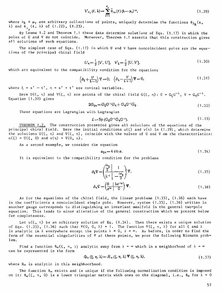
V.r (t, ~)= E ~rs (t) (%--~r) -s, ( 1 . 2 9 ) S o l

where X k ~ ~r are arbitrary collections of points, uniquely determine the functions CXk(X, X) and (t, X) of (1.22), (1.23).

r By Lemma 1.2 and Theorem 1.1 these data determine solutions of Eqs. (1.17) in which the

poles of U and V do not coincide. Moreover, Theorem 1.1 asserts that this construction gives all solutions of such equations.

The simplest case of Eqs. (1.17) in which U and V have noncoincident poles are the equations of the principal chiral field

�9 1 I [U, V], (1 .30) U ~ = ~ [V, U], V~----

which are equivalent to the compatibility condition for the equations

--~--~) ----0, (I .31)

where ~ = x' -- t' ' t' , q = x + are conical variables.

Here U(~, q) and V(~, ~) are points of the chiral field G(r n): U = G~G -I, V = G~G -z. Equation (1.30) gives

2G~=G~G-~G~+O~G-~G~ �9 (1.32)

These equations are Lagrangian with Lagrangian

L=Sp (G~G-~G~G-~). (1.33) THEOREM 1.2. The construction presented gives all solutions of the equations of the

principal chiral field. Here the initial conditions u(~) and v(o) in (1.29), which determine the solutions U(~, q) and V(~, ~), coincide with the values of U and V on the characteristics: u(~) = U(~, 0) and v(n) = V(0, n).

As a second example, we consider the equation

u ~ = 4 s l n u . ( 1 . 3 4 )

It is equivalent to the compatibility condition for the problems

�9 , (1.35)

I (1.36)

As f o r the equat ions of the c h i r a l f i e l d , the l i n e a r problems (1 .35) , (1.36) each have in the coefficients a noncoincident simple pole. However, system (1.35), (1.36) written in another gauge corresponds to distinguishing an invariant manifold in the general two-pole equation. This leads to minor alteration of the general construction which we present below for completeness.

Let u(~, n) be an arbitrary solution of Eq. (1.34). Then there exists a unique solution of Eqs. (1.35), (1.36) such that ~(0, 0, X) = I . The function $(6, q, X) for all ~ and X is analytic in X everywhere except the points X = 0, X = ~. As before, in order to find the form of the essential singularities of ~ at these points, we pose the following Riemann problem.

Find a function r ~, ~) analytic away from X = ~ which in a neighborhood of X = can be represented in the form

~ ( ~ , ~, ~ ) = ~ ( ~ , ~, ~) ~ (~, ~, ~), ( I .37)

where P~o is analytic in this neighboorhood.

The function r exists and is unique if the following normalization condition is imposed on it: ~(~, ~, 0) is a lower triangular matrix with ones on the diagonal, i.e., r for X = 0

57

has the form

�9 o, o) I (1.38)

These are three linear conditions on ~=. We impose still another condition by requiring that P~o(~, q, =) be an upper triangular matrix. Since det~ = I, it follows that l~o(~, q, ~) has the form

n, - W Ig-')" (1 .39)

We consider the logarithmic derivatives of @=. It follows from (1.37) that in a neighborhood of % =

(a~qI-)o~l:a~R-a=l-I - a - L_I I i~, R : I. (1.4o) - - T

Hence ~.@~1 is regular in a neighborhood of X = ~, and its value at this point is an upper triangular matrix. Since ~r is regular everywhere, it is constant. Moreover, it follows from (I~38) that

( ~ ~ �9 (1.41)

Hence ~ = 0.

Since ~oo does not depend on ~, it follows that

~ ( ' q , ~ ) = R ~ ( O , "q, * )~ (0 , "q, ~,). (1.42)

The function ~(0, q, %) has only one essential singular point % = =o, and it satisfies condition (I .38). From the uniqueness of @oo it follows that

~)=(N, ~)----- IF (O, N, %). (I .43)

It follows from (1.36) that ~oo(n, ~) satisfies the equation ~e_lu, \

e'u, , 0 ) (1.44)

where ul(q) = u(0, ~).

We consider in a similar way the function ~0(~, n, X) regular in the entire extended complex plane except at the point % = 0; in a neighborhood of this point it can be represented in the form

~o(~, ~1, %)---Ro(~,, 11, ~.)~[r ((~, ~], %,), (1.45)

where R0 is regular in this neighborhood.

We choose the following normalization conditions uniquely determining ~0. The matrix ~0(~, q, o~) is upper triangular, and R0(~, q, O) has the form (1.38).

In a neighborhood of X = 0 we have, according to (I .45),

0 ~.e-~"\ , OnO~176 + R~ e i" 0 )Ro . (I .46)

This implies that ~qO0~ I is regular everywhere and is hence constant. From the normalization conditions and (1.46) it follows that ~q@0~oll%=0 can have only the left lower element nonzero. It is equal to zero, since ~0(~, q, ~) is upper triangular. Hence ~0 = 0 or ~0(~, n , x) = ~ o ( r %). 0, %) and

i u where ~(~)=~- g(cj, 0).

58

Repeating literally the arguments for ~oo, we find that ~0($, %) = ~(~,

b~CDo=( ~ 1 w/-I)o, ~-, _,. (1 .47)

We have thus proved the following result.

LEMMA 1.3. The solutions @= and r of the Riemann problems posed depend only on q and ~, respectively, ~ = @~(q, %), ~0 = r %), and satisfy Eqs. (1.44), (1.47).

We now consider the inverse problem. Suppose there are given two arbitrary functions ul(q) and w(~). We define ~=(n, %) and @0(~, %) as solutions of Eqs. (1.44) and (1.47), respectively, with the initial conditions r %) = @0(0, %) = I.

Suppose that ~(~, n, %) is a regular function of % away from the points % = 0 and % = in neighborhoods of which it has the form

V(~, ll, %)=R0(~, N, X)~0(~, %), (1.48) �9 (~, ~, ~ ) = ~ ( ~ , ~, ~)~(~, x),

where R0 and ~ are r e g u l a r ma t r ix f u n c t i o n s in the cor responding ne ighborhoods .

The f u n c t i o n ~ e x i s t s and i s unique i f we a d d i t i o n a l l y r e q u i r e t h a t ~1%=~ and R01%= 0 have the form

THEOREM 1.3. The function ~(~, n, %) satisfies Eqs. (1.35), (1.36) where u(~, n) = u1(q) -- 2iing(~, q). Here u(E, q) is a solution of Eq. (1.34). All solutions of this equation are given by the proposed construction.

The proof of the theorem follows from considerations connected with the analysis of the logarithmic derivatives of P which have already been used repeatedly.

It should be noted that construction of local solutions of the sine-Gordon equation depending on two arbitrary functions was proposed in the work [61]. The solutions are represented in the form of series whose convergence is proved by means of the theory of infinite- dimensional Lie algebras. Here there was originally no connection of the functional parameters figuring in this construction with the initial data of problems of Goursat type. Recently [62] this gap was partially filled.

2. "Finite-Zone Solutions" of Equations Admitting a Representation

of Zero Curvature

The purpose of the present section is to distinguish algebrogeometric or "finite-zone" solutions of general equations admitting a representation of zero curvature. As in the preceding section, we consider Eqs. (1.17) without specifying the gauge and without carrying out reduction of the general system to some invariant submanifolds.

The restriction of system (1.17) to equations describing finite-zone solutions is carried out by means of an additional condition which is equivalent to the imbedding of Eqs. (1.17) in an extended system.

Definition. "Finite-zone solutions" of Eqs. (1.17) are solutions U(x, t, %) and V(x, t, %) of these equations for which there exists a matrix function W(x, t, %) meromorphic in % such that the following equations are satisfied:

[a~,-u, w]=0 , [a,-v, W l = 0 (1.50)

As p r e v i o u s l y , we cons ide r a s o l u t i o n ~(x, t , %) of Eqs. (1 .15 ) , (1.16) normal ized by the c o n d i t i o n ~(0, 0, %) = 1.

I t f o l l ows from ( ] .50) t h a t W(x, t , %)~(x, t , %) a l s o s a t i s f i e s Eqs. (1 .15 ) , ( 1 .16 ) . Since a s o l u t i o n of the l a t t e r system is un ique ly de termined by the i n i t i a l c o n d i t i o n , i t f o l l ows t h a t

IV(x, t, X)V(x, t, X)=~F(x, t, X)IV(O, O, ~). (1.51)

Hence, the c o e f f i c i e n t s of the polynomial

Q(X, F) = det (IV (x, t, X)--F.I) (1.52)

do not depend on x and t . They a re i n t e g r a l s of Eqs. ( 1 . 50 ) .

59

It will henceforth be assumed that for almost all X the matrix W(O, 0, X) has distinct eigenvalues, i.e., the equation

Q(~, ~)=0 ( 1 . 5 3 )

defines in C 2 the affine part of an algebraic curve F which is ramified in ~-sheeted fashion over the X plane where ~ is the dimension of the matrices U, V, W. The corresponding solutions are called finite-zone solutions of rank I.

Remark. A description of finite-zone solutions of ranks higher than I [here the polynomial Q(X, ~) = Qr(x, A), where r is the rank of the solution] for the Kadomtsev--Petviashvili equation and the theory connected with this which is based on the possibility of applying the apparatus and language of the theory of multidimensional holomorphic bundles over algebraic curves can be found in [35-37].

If the roots of Eq. (1.53) are simple for almost all X, then to each such root, i.e., each point y = (X, ~) of the curve F, there corresponds a unique eigenvector h(y),

W(O, O, x) hC~)=~h(~), (1.54)

which is normalized since its first coordinate hi(y) =- I. The remaining coordinates hi( Y ) are hereby meromorphic functions on F.

Suppose that ~i(x, t, X) is the i-th column vector of the matrix ~(x, t, X). We consider the solution ~(x, t, y) of Eqs. (1.15), (1.16) given by the formula

t

, (x, t, v) = ~ h, (v) v ' (x, t, ~). (1.55)

We d e n o t e by Pa, a = 1 , . . . , Z ( n + m), t he p re images on Y of the p o i n t s ~r and Xk -- the p o l e s of V and U. Then, s i n c e ~(x , t , X) i s a n a l y t i c away from the p o i n t s Xk, Vr, i t f o l l o w s that ~(x, t, y) is meromorphic on F away from the points Pa. The divisor of its poles O coincides with the divisor of poles of h(y).

(Here and below a divisor is simply a collection of points with multiplicities.)

In order to find the form of the singularities of ~(x, t, y) at the points Pa, we use the fact that by (1.51)

IJU(x, t, ~ )~(x , t, "f) ---- l ~ (X, t, ~). ( 1 .56 )

Hence,

(x, t, v) - - f (x, t, v) k (x, t, v), ( 1 .57)

where f ( x , t , u i s a s c a l a r f u n c t i o n , and h ( x , t , u i s an e i g e n v e c t o r o f the m a t r i x W n o r - m a l i z e d by the condition h1(x , t, y) = 1. As in the case of h(y), all the remaining coordinates hi(x , t, y) are meromorphic functions on F.

We consider the matrix ~(x, t, X) whose columns are the vectors ~(x, t, u where yj = (X, ~j) are the preimages of the point X on the curve F. This matrix is uniquely determined up to a permutation of columns. From (1.57) we have

~ ( x , t, ~ ) = / ~ ( x , t, ~)P(x , t, ~), (1.58)

where the matrix H is constructed from the vectors h(x, t, u in the same way as ~, the matrix F is diagonal, and its elements are equal to f(x, t, yj)6ij.

Since ~(x, t, y) satisfies Eqs. (1.15), (1.16), it follows that

U (x, t, X) = qx ~-I = HxH- ' + I-fFx F-ll-f-l, (1 .59 )

V(x, t, ~) = ~ , q - ' " t~,~7-, + /~FtF- ' / : / -1 . ( 1 .60)

Hence, in a neighborhood of the points Pa the function f(x, t, y) has the form

f ( x , t, ?)----exp(q=(x, t, k~)) f~(x , t, y), (1 .61 )

where q (x , t , k) i s a p o l y n o m i a l i n k , f a ( x , t , y) i s a meromorphic f u n c t i o n in a n e i g h b o r h o o d of P~, and k~1(u i s t h e l o c a l p a r a m e t e r i n n e i g h b o r h o o d s of the p o i n t s k ~ l ( P~ ) = 0.

Su~arizing, we arrive at the following assertion.

60

THEOREM 1.4. The vector-valued function ~(x, t, y).

I) It is meromorphic on F away from the points P~. Its divisor of poles does not depend on x, t. If W is nondegenerate, then in general position it my be assumed that the curve F is nonsingular. Here the degree of the divisor of poles of * is equal to g + ~ -- I, where g is the genus of the curve F.

2) In a neighborhood of the point P~@(x, t, y) has the form

~ ( x , r ~ ) = s~(X, t)k~' exp(q~(x, l, k~), ( 1 . 6 2 )

where t h e f i r s t f a c t o r i s t h e e x p a n s i o n in a n e i g h b o r h o o d of Pa in t e r m s of t h e l o c a l p a r a m - e t e r k~ ~ = k ~ l ( u o f some m e r o m o r p h i c v e c t o r , and q ~ ( x , t , k) i s a p o l y n o m i a l i n k . I f U ( o r V) h a s no p o i e a t t h e p o i n t X which i s t h e p r o j e c t i o n o f Pa o n t o t he X p l a n e , t h e n qa does n o t depend on x ( o r t ) .

The o n l y a s s e r t i o n of t h e t h e o r e m n o t p r o v e d above r e g a r d i n g t h e number of p o l e s o f ~ f o l l o w s f r o m t h e f a c t t h a t ( d e t ~ ) 2 i s a w e l l - d e f i n e d m e r o m o r p h i c f u n c t i o n of X. T h e p o l e s o f t h i s f u n c t i o n c o i n c i d e w i t h t h e p r o j e c t i o n s o f t h e p o I e s of h ( y ) , i . e . , w i t h t h e p r o j e c t i o n s of t h e p o l e s of ~, w h i l e t h e z e r o s c o i n c i d e w i t h t h e images of t h e b r a n c h p o i n t s o f F, i . e . , w i t h p o i n t s a t which e i g e n v a l u e s of W(O, 0, X) c o a l e s c e . We h a v e 2N = u, where N i s t h e number of p o l e s of ~ and u i s t h e number of b r a n c h p o i n t s o f F ( b o t h c o u n t i n g m u l t i p l i c i t i e s ) . Us ing t h e f o r m u l a [46]

2g--2 : v--2l, ( 1 . 6 3 )

c o n n e c t i n g the genus of an ~ - s h e e t e d c o v e r i n g of t h e p l a n e w i t h t h e number of b r a n c h p o i n t s , we o b t a i n

N = g + l - - l . ( 1 . 6 4 )

A x i o m a t i z a t i o n of t h e a n a l y t i c p r o p e r t i e s of ~ ( x , t , y) e s t a b l i s h e d in Theorem 1.4 f o r m s t h e b a s i s f o r t he c o n c e p t o f t he B a k e r - - A k h i e z e r f u n c t i o n which i s p e r h a p s t h e c e n t r a l c o n c e p t i n t h e a l g e b r o g e o m e t r i c v e r s i o n o f t h e method of t h e i n v e r s e p r o b l e m .

A g e n e r a l d e f i n i t i o n o f such f u n c t i o n s was g i v e n i n [ 2 6 ] .

I n a n e i g h b o r h o o d of p o i n t s P 1 , . . - , P M of a n o n s i n g u l a r c u r v e F we f i x l o c a l p a r a m e t e r s k ~ l ( u k ~ l ( P a ) = O. I n a n a l o g y w i t h t h e s p a c e ~ ( D ) of m e r o m o r p h i c f u n c t i o n s on F a s s o - c i a t e d w i t h a d i v i s o r D, f ( y ) 6 ~ ( ~ ) ) , i f D + Df ~ 0, where Df i s t h e p r i n c i p a l d i v i s o r of f , we i n t r o d u c e the s p a c e A(q, D) , where q i s a c o l l e c t i o n of p o l y n o m i a l s q ~ ( k ) .

A f u n c t i o n ~ ( q , y) b e l o n g s to ^ ( q , y) i f

1) away f r o m t h e p o i n t s Pa i t i s m e r o m o r p h i c , w h i l e f o r t h e d i v i s o r of i t s p o l e s D~ ( t h e m u l t i p l i c i t y w i t h wh ich t h e p o i n t Ys i s c o n t a i n e d in D i s e q u a l w i t h a minus s i g n t o t h e m u l t i p l i c i t y o f t h e p o l e of t h e f u n c t i o n a t t h i s p o i n t ) we h a v e D~ + D ~ O;

2) i n a n e i g h b o r h o o d of Pa t h e f u n c t i o n ~ ( q , y) exp ( - - q ~ ( k ~ ( y ) ) i s a n a l t y i c , k ~ l ( P ~ ) = O.

THEOREM 1 .5 . Fo r a n o n s p e c i a l d i v i s o r D ) 0 o f d e g r e e N ) g d i m A ( q , D) = N -- g + 1.

We r e c a l l t h a t t h o s e d i v i s o r s f o r which d i m ~ ( D ) = N - - g ~ l a r e c a l l e d n o n s p e c i a l d i v i s o r s f o r m i n g an open s e t among a l l d i v i s o r s .

I n some s p e c i a l c a s e s t h i s a s s e r t i o n was f i r s t p r o v e d by Bake r and A k h i e z e r [1 , 5 2 ] . T h e r e f o r e , f u n c t i o n s o f t h i s t y p e a r e c a l l e d B a k e r - - A k h i e z e r f u n c t i o n s . The method o f p r o o f of t h i s a s s e r t i o n u s e d i n t h e work [1] ( s e e a l s o [14 , 23]) i s b a s e d on t h e f a c t t h a t d~ /~ i s an A b e l i a n d i f f e r e n t i a l on F. To c o n s i d e r a b l e e x t e n t t h e p r o o f r e p e a t e d t h e c o u r s e of t h e p r o o f o f A b e l ' s t h e o r e m and t h e s o l u t i o n o f t h e J a c o b i i n v e r s i o n p r o b l e m [ 2 1 ] .

The e x p l i c i t c o n s t r u c t i o n o f ~ ( q , D) i s t h e s i m p l e s t and a t t h e same t i m e mos t e f f e c t i v e means of p r o v i n g t h e t h e o r e m .

On a n o n s i n g u l a r a l g e b r a i c c u r v e F of genus g we f i x a b a s i s o f c y c l e s

a~ . . . . . a a ; b~ . . . . . b e

with intersection matrix a~oai=biob j, a~obj=~t~. We introduce the basis of holomorphic dif-

normalized by the conditions ~;=~ . We denote by B the matrix of b ferentials ~k on r

61

periods Bik=~k. It is known that it is symmetric and has positive-definite imaginary b i

part.

Integral combinations of vectors in cg with coordinates 6jk and Bik form a lattice de- fining a complex torus J(F) called the Jacobi manifold of the curve.

Let P0 be a distinguished point on F; then the mapping A:F § J(F) is defined. The co-

ordinates of the vector A(y) are equal to ~flk. P0

On the basis of the matrix of b periods, just as for any matrix with positive-definite imaginary part, it is possible to construct an entire function of g complex variables

O(tt, . . . . . tt,,) = ~,~ exp(~i(Bk, k)+2:~i(k , tt)), kCzg

where (k , u) = k lUl + . . . + kgug .

It possesses the following easily verified properties:

0 (ttl . . . . . ttj--}- 1, ttj+l . . . . ttg) = 0 (U, . . . . . U i . . . . t tg) ,

(I .65) 0 (ul q- B1k ..... ueq- Bg~) = exp (~i (Bk~q- 2Uk)) 0 (Ul ..... Ug).

Moreover, for any nonspecial effect divisor D = YI +... + yg of degree g there exists a vector Z(D) such that the function 0(A(y) + Z(D)) defined on F dissected along the cycles ai, bj has exactly g zeros coinciding with the points Yi (see [21]),

z~(b)=- A~(,C,)+~--~e~+~ a~, tea~. s--I j4d~ a~

For any collection of polynomials qa(k) there exists a unique Abelian differential of second kind (see [44]) m (the index of mq we omit to simplify notation) having a singularity at the distinguished point P~ on F of the form dq~(k~) in the local parameter k~ 1 and normal-

ized by the conditions ~ r

a i

LEMMA 1.4. Let D be an arbitrary effective, nonspecial divisor of degree g; then the function

~(q , y ) = e x p ( S o~ 0 ( A ( v ) + z ( b ) + o ) ( 1 . 6 6 ) ,~ j o ( a ( ~ ) + z ( b ) ) '

where U = (U1 , . ,Ug) and U k ~ l . . ~ ~ i s a g e n e r a t o r of a o n e - d i m e n s i o n a l space A(q, D). b k

The p r o o f o f t h e lemma f o l l o w s f rom a s i m p l e v e r i f i c a t i o n of t h e p r o p e r t i e s o f t h e f u n c - t i o n ~ ( q , y ) . I t f o l l o w s d i r e c t l y f rom t h e p r o p e r t i e s ( ] . 6 5 ) t h a t t h e r i g h t s i d e of Eq. ( 1 . 6 6 ) g i v e s a w e l l - d e f i n e d f u n c t i o n on F, i . e . , i t s v a l u e s do n o t change on p a s s i n g a round t h e c y c l e s ai , b j . In a n e i g h b o r h o o d of Pa the f u n t i o n ~, as f o l l o w s f rom th e d e f i n i t i o n of m, has t he r e q u i r e d e s s e n t i a l s i n g u l a r i t y (a f o r m u l a o f t h i s t y p e f o r t h e B loch f u n c t i o n of t h e f i n i t e - z o n e S c h r U d i n g e r o p e r a t o r was f i r s t o b t a i n e d by I t s [ 2 3 ] ) .

The fact that A(q, D) is one-dimensional follows from the fact that if ~IEK(q, D), then ~i/~ is a meromorphic function on F with g poles. By the Riemann--Roch theorem and the fact that the divisor is nonspecial we find that ~l/~ = const.

To complete the proof of the theorem it suffices to note that functions ~i(q, Y) of the form (1.66) corresponding to divisors D i = Y1 + ... + Yg-i + Yg+i (where D = YI + ... + YN ) form a basis of the space A(q, D).

By Theorem 1.4 to each finite-zone solutions of Eqs. (1.17) of rank I there correspond a curve F, which can be assumed nonsingular in general position, a collection of polynomials qa(x, t, k), and a nonspecial divisor of degree g + I -- I, where g is the genus of the curve. We shall use the preceding theorem to construct an inverse mapping.

62

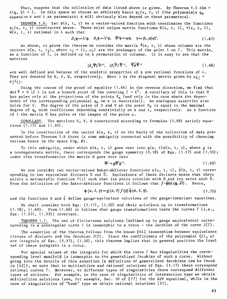
Thus, suppose that the collection of data listed above is given. By Theorem 1.5 dim • A(q, D) = ~. In this space we choose an arbitrary basis ~i(x, t, y) (the polynomials q~ depend onx and t as parameters; ~ will obviously also depend on these parameters).

THEOREM 1.6. Let ~(x, t, y) be a vector-valued function with coordinates the functions ~i(x, t, y) constructed above. There exist unique matrix functions U(x, t, %), V(x, t, %), W(x, t, %) rational in % such that

ax~:U~, Ot~-=V ~, W ~ = ~ , Y:~,~)EP. (1.67)

As above, to prove the theorem we consider the matrix ~(x, t, ~) whose columns are the vectors ~(x, t, yj), where yj = (%, ~j) are the preimages of the point % on F. This matrix, as a function of %, is defined up to a permutation of columns. It is easy to see that the matrices

(aXe) ~_l (al~)~-l ~ - - l (1.68)

are well defined and because of the analytic properties of ~ are rational functions of ~. They are denoted by U, V, W, respectively. Here ~ is the diagonal matrix given by ~ij =

~j6ij.

Using the course of the proof of equality (1.64) in the reverse direction, we find that det~ = 0 if % is not a branch point of the covering r § C I. A corollary of this is that U has poles only at the projections of the points Pa (and only in the case where the dependence of the corresponding polynomial q~ on x is nontrivial). An analogous assertion also holds for V. The degree of the poles of U and V at the point Pa is equal to the maximal degree of q~ with coefficient depending nontrivially on x and t, respectively. As a function of % the matrix W has poles at the images of the poles ~.

COROLLARY. The matrices U, V, W constructed according to formulas (1.68) satisfy equations (1.17) and (1.50).

In the construction of the vector ~(x, t, y) on the basis of the collection of data presented before Theorem 1.6 there is some ambiguity connected with the possibility of choosing various bases in the space A(q, D).

To this ambiguity, under which ~(x, t, y) goes over into g(x, t)~(x, t, y), where g is a nondegenerate matrix, there corresponds the gauge symmetry (1.18) of Eqs. (1.17) and (1.50); under this transformation the matrix W goes over into

W--+gWg -I. ( I .69)

We now c o n s i d e r two v e c t o r - v a l u e d Baker - -Akhiezer f u n c t i o n s $ ( x , t , y ) , ~ (x , t , y) c o r r e - s p o n d i n g to two equivalent divisors D and D. Equivalence of these divisors means that there exists a meromorphic function f(y) such that its poles coincide with D and its zeros with D. From the definition of the Baker--Akhiezer functions it follows that f.~EACq, D) . Hence,

~(X, t, ~ : g ( X , t) y(v)~(X, t, V), (1 .70 )

and the f u n c t i o n s ~ and ~ d e f i n e g a u g e - e q u i v a l e n t s o l u t i o n s o f t h e g a u g e - i n v a r i a n t e q u a t i o n s .

We s h a l l c o n s i d e r b o t h Eqs. ( 1 . 1 7 ) , (1 .50 ) and t h e i r s o l u t i o n s up to t r a n s f o r m a t i o n s ( 1 . 1 8 ) , ( 1 . 6 9 ) . From ( 1 . 6 9 ) i t f o l l o w s t h a t gauge t r a n s f o r m a t i o n s l e a v e the c u r v e s F [ i . e . , Eqs. ( 1 . 5 2 ) , ( 1 . 5 3 ) ] i n v a r i a n t .

THEOREM 1.7 . The s e t of f i n i t e - z o n e s o l u t i o n s ( d e f i n e d up to gauge e q u i v a l e n c e ) c o r r e - s p o n d i n g to a n o n s i n g u l a r c u r v e F i s i s o m o r p h i c to a t o r u s -- t he J a c o b i a n o f t he c u r v e J ( r ) .

The assertion of the theorem follows from the known [44] isomorphism between equivalence classes of divisors and the Jacobian J(F). Since the coefficients of the polynomial Q(%, ~) are integrals of Eqs. (1.17), (1.50), this theorem implies that in general position the level set of these integrals is a torus.

For special values of the integrals for which the curve F has singularities the corresponding level manifold is isomorphic to the generalized Jacobian of such a curve. Without going into the details of this assertion (a definition of generalized Jacobians can be found in [42]), we note that to multisoliton and rational solutions of Eqs. (1.17) there correspond rational curves F. Moreover, to different types of singularities there correspond different types of solitons. For example, in the case of singularities of intersection type we obtain multisoliton solutions (see, for example, Sec. 10 of [17] for the KdV equation), while in the case of singularities of "beak" type we obtain rational solutions [31].

63

So far we have discussed the general equations (1.17). Conditions imposed on U and V to distinguish invariant submanifolds of these equations lead to corresponding conditions on the parameters of the construction of finite-zone solutions of these equations.

We shall consider these conditions for the example of the sine-Gordon equation. Finite- zone solutions of this equation, which has, in addition to the representation (1.17) with matrices (1.35), (1.36) also the ordinary representation (1.2) with (4 x 4)-matrix operators, were first constructed in [24]. Subsequently, application of the general construction of finite-zone solutions proposed by the author [32] was carried out in application to the sine-

Gordon equation in [22] (see also [45, 46]).

It may be assumed with no loss of generality that W(~, q, %) does not have poles at the points % = 0 and % = =, since this can always be achieved by multiplying W by a constant

rational function of %.

Since the left sides of the equations

W~=[W,U], W~=IW, V], (1.71)

which coincide with (1.50), do not have poles for X = 0, X = =, it follows from the form of U

and V (1.35), (1.36) that

O0 O l

Hence, W(~, ~, X) in a neighborhood of these po in ts has the form

/ I \ w ~ 0 W (~' " X) = [~"([~,) + 0 (%)' (1.72)

t W j w, , (I w (TIT,,)+ O 73)

Hence, the curve F defined by the characteristic equation (1.53)

b 2 - r i ~) F + r2 (X) = 0 , ( 1 . 7 4 )

rz : Sp W, r2 : det W, branches at the points % = 0 and % = =. It also follows from (1.72),

(1.73) that

h2(~, ~, ~ ) = 0 ; h2(~,~, ~)=OCX-,n), x~O, (1.75)

where, as p rev i ous l y , h i (E , q, ~) are coord inates of an e igenvector of W(~, n, ~) normalized by the condition hz = I.

With consideration of these remarks Theorem 1.4 assigns to each finite-zone solution of the sine-Gordon equation of hyperelliptic curve F (1.74) with two distinguished branch points P0 and P= situated over ~ = 0 and ~ = = and also a divisor Do of degree g.

Away from the points P0 and P= the corresponding Baker--Akhiezer functions have g poles at points of the divisor Do. In a neighborhood of P0 they have the form

~'(~'~'k)=ek~(l+2x~'(~'~)k-s) ' s = . .2(~, n, k) = e k ~ l + ~ x . ~ ( ~ , n)~ -~ , (1 .76)

where k = ~-i/2

In a neighborhood of Poo we have

, , (vj, n, k) = c~e*'~ I + q , (~, n) k-" ,

* 2 ( ~ , ' q , k ) = c 2 e ~ k -~ 1 + ~2(~, k -~ 1

(1.77)

where k = %z/2 c i = ci(E, q)

64

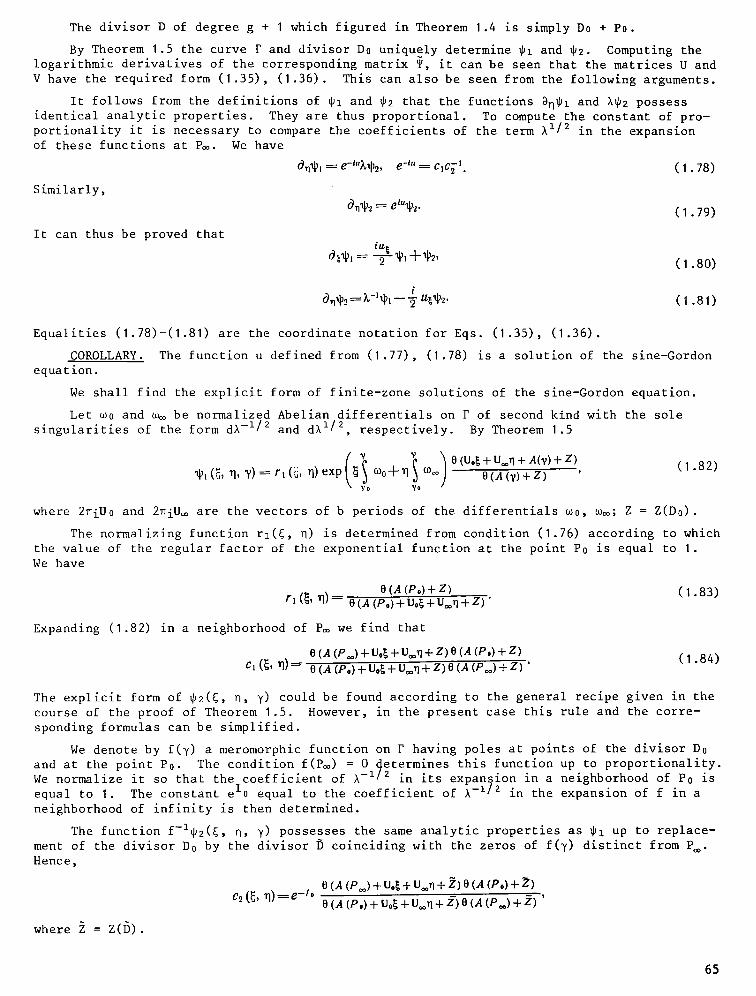
The divisor D of degree g + I which figured in Theorem 1.4 is simply Do + P0.

By Theorem 1.5 the curve F and divisor Do uniquely determine ~l and ~2. Computing the logarithmic derivatives of the corresponding matrix ~, it can be seen that the matrices U and V have the required form (1.35), (1.36). This can also be seen from the following arguments.

It follows from the definitions of ~I and ~2 that the functions a~l and X~2 possess identical analytic properties. They are thus proportional. To compute the constant of proportionality it is necessary to compare the coefficients of the term X~/2 in the expansion of these functions at P~. We have

an~, ---- e-~"k~, e -~" ----- clc~ I. ( 1 . 78)

Similarly,

It can thus be proved that

On~. 2 = et.~2. ( I. 79)

( i . 8o)

i (1.81)

Equalities (1.78)-(1.81) are the coordinate notation for Eqs. (1.35), (1.36).

COROLLARY. The function u defined from (1.77), (1.78) is a solution of the sine-Gordon equation.

We shall find the explicit form of finite-zone solutions of the sine-Gordon equation.

Let w0 and 0~o be normalized Abelian differentials on F of second kind with the sole singularities of the form dX -I/2 and dX I/2, respectively. By Theorem 1.5

~t(~, 11, ~ ) = r , ( ~ j , ~ )exp ~ m 0 + ~ m= 8 ( A ( ? ) + Z ) "' ( 1 . 8 2 ) yo

where 2wiU0 and 2~iU~ a r e t h e v e c t o r s o f b p e r i o d s o f t h e d i f f e r e n t i a l s m0, m~; Z = Z ( D 0 ) .

The n o r m a l i z i n g f u n c t i o n r z ( g , n) i s d e t e r m i n e d f r o m c o n d i t i o n ( 1 . 7 6 ) a c c o r d i n g t o w h i c h t h e v a l u e o f t h e r e g u l a r f a c t o r o f t h e e x p o n e n t i a l f u n c t i o n a t t h e p o i n t P0 i s e q u a l t o 1. We have

e (A (P~ + Z) r~ (~, n) = o (A (P~ + Uo~ + u=n + z )"

Expanding (1.82) in a neighborhood of P= we find that

8 (A (P~) + Uo[ + IJ=jI + Z) 8 (A (Po) + Z) cl (~, ~1) ----- e (A (Po) + Uo[ + U~I + Z) 0 (A (P~) + Z) "

(1.83)

(1.84)

The explicit form of ~2(~, ~, y) could be found according to the general recipe given in the course of the proof of Theorem 1.5. However, in the present case this rule and the corresponding formulas can be simplified.

We denote by f(y) a meromorphic function on F having poles at points of the divisor Do and at the point Po. The condition f(P=) = 0 determines this function up to proportionality. We normalize it so that the coefficient of X -1/2 in its expansion in a neighborhood of Po is equal to I. The constant elo equal to the coefficient of X-z/2 in the expansion of f in a neighborhood of infinity is then determined.

The function f-l~2(~, n, Y) possesses the same analytic properties as ~z up to replace- ment of the divisor Do by the divisor D coinciding with the zeros of f(y) distinct from P~. Hence,

0 (A (P~) + Uo~ + u~n + 2) e (A (P0) + 2) c2 (~, ~) = e - ' ~

o (A (Po) + u~ + U~n + f) 0 (A (P~) + 2) '

where Z = Z(D).

65

The divisors Do + P0 and D + P~ are equivalent. Therefore, by Abel's theorem [44]

Z q- A (Po) = 2 q- A (P~) .

I t f o l l o w s f r o m t h i s t h e o r e m t h a t t h e v e c t o r a = A(P~) -- A(P0) i s a h a l f p e r i o d , s i n c e 2P0 a n d 2P= a r e e q u i v a l e n t ( t h e f u n c t i o n X h a s a p o l e o f s e c o n d o r d e r a t P~ and a z e r o of m u l t i - p l i c i t y 2 a t P 0 ) .

We arrive finally at the formula

o= (w + Uo~ + u~n) o (w--a) 0 (w + a) ( 1 .85 ) e tu ~ e - - l o ,

0 (W--A + uo~ + U ~ ) 0 (W + a + U0~ + u ~ ) 0=(W)

f o r f i n i t e - z o n e s o l u t i o n s o f t h e s i n e - G o r d o n e q u a t i o n . I n t h i s f o r m u l a W = Z(D0) + A ( P 0 ) . However, this vector may be assumed arbitrary, since as Do varies the vectors W fill out the entire Jacobian.

In this chapter we have not touched on the important question concerning distinguishing real finite-zone solutions not having singularities. It is rather trivial to distinguish real solutions in those cases where the operators whose commutativity condition is equivalent to the equation considered are self-adjoint. In this case an antiinvolution is defined naturally on the curve P, and real solutions correspond to data invariant under this antiinvolution.

For non-self-adjoint operators the problem is considerably more complicated. Conditions that solutions (1.85) of the sine-Gordon equation be real were described in [45, 46]. Effec- tivization of these conditions and completion of the question regarding realness of finite- zone solutions (1.85) were accomplished in [16].

3. Representations of "Zero Curvature" and Elliptic Curves

Recently active attempts have been made to generalize Eqs. (1.17) to the case of pencils in which the matrices U and V are meromorphic functions of a parameter % defined on an algebraic curve F of genus greater than zero. (The case of rational pencils corresponds to g = 0.) We note that the Riemann--Roch theorem impedes the automatic transfer of Eqs. (1.17) to a curve of genus g > O.

Indeed, suppose that U(x, t, %) and V(x, t, X) are meromorphic functions on P, %EF. having divisors of poles of multiplicity N and M. Then by the Riemann--Roch theorem [46] the number of independent variables is equal to Z2(N -- g + I) for U and ~2(M -- g + I) for V (where ~ is the dimension of the matrices). The commutator [U, V] has poles of total multiplicity N + M. Therefore, Eqs. (I.|7) are equivalent to ~2(N + M -- g + I) equations for the unknown functions. With consideration of gauge symmetry (1.18) for g ~ I the number of equations is always greater than the number of unknowns.

There are two ways to circumvent this obstacle. One way is proposed in the work [35] where, in addition to poles fixed relative to x and t, the matrices U and V admit poles depending on x, t in a particular manner. It was shown that the number of equations [with consideration of (1.18)] hereby coincides with the number of independent variables which are the singular parts of U and V at the fixed peles. Since no physically interesting equations have so far been found in this scheme, we shall not consider it in more detail.

The second way is based on a choice of a special form of the matrices U and V and has been successfully realized only in some examples on elliptic curves P (g = I). The physically most interesting example of such equations is the Landau--Lifshits equation

S j = S X Sxx+S X IS, ( 1 . 8 6 )

where S is a three-dimensional vector of unit length, 1~1 = I, and lab = I~6~B is a diagonal matrix. It was shown in the work [67] that Eq. (1.86) is the compatibility condition for linear equations (1.15), (1.16) where the 2 x 2 matrices U and V are

8

u = s= (x, (i .87)

8

v = - i b = a= s=o=, (1 .8a)

66

where

P w t = b l = sn(~,k); ~02=b2~= p dn(%, k). sn (X, k) '

cn(~, k). (1 .89) '~z=bz=p sn(%, k) ' a,=--qf)2~)3, 52=--~)3~)1 ,

aa=--~v,~2; sn(X,k), cn(l,k), dn(~,k)

are Jacobi elliptic functions [2], and o e are the Pauli matrices.

The parameters Ia are given by the relations

k = ]/2/r7~ 1 ( I. 90) g 4--,-,---77,' P=~ 1/ la- I ' ' 0 < k < l .

In [47, 64] multisoliton solutions of these equations were constructed, and attempts were made to construct finite-zone solutions; these attempts have so far not given an effective answer.

The pair (1.87), (1.88) has 4 poles on the curve F. It turns out that Eq. (1.86) can be represented in the form of a commutation condition of "single-pole pencils" if in U and V we give up the condition that the pencils be meromorphic on the entire curve F.

We fix an elliptic curve F and an l-dimensional vector z = (zl ..... z~), z i ~ zj. We denote by G(F, z) the infinite-dimensional algebra of matrix-valued functions U(%) such that

I) they are meromorphic away from the point % = 0;

2) in a neighborhood of % = 0 the matrix element of U has the form

U/i (~) = exp (ff_~O ~;~-s (1.91)

(henceforth z i -- zj is denoted by zij). Conditions I) and 2) mean that the matrix elements are functions of Baker--Akhiezer type.

For any divisor of degree N the dimension of the linear space of matrix functions of the type described having poles at the points of this divisor is equal to N~ 2 . As in the case of rational pencils, it is possible to take as independent parameters the singular terms of U(%).

For example, suppose that U(%) has simple poles at the points %~,...,%N; then

N "

Ulj (%) = ~ ~j(D (ZIj, %,, %k)' ( 1 .92 ) 4=1

where

! I \

r x, ~ ) - e :~x~ = [ ~_-Z:-~; + . . . ) e~(X)z (1 .93) (X- -kn ) a (z)

i s the s i m p l e s t f u n c t i o n of Baker--Akhiezer type (he re o, ~ a re the W e i e r s t r a s s f u n c t i o n s [ 2 ] ) .

For the diagonal elements we have

N N

g u ( ~ ) = u t o - l - E u l ~ ( ~ - - ~ k ) , ~.~ uik=O. (1 .94) k=l k=l

A s s e r t i o n . Suppose t h a t U(~, n, ~) and V(~, n, ~) a re m a t r i x - v a l u e d f u n c t i o n s be long ing f o r a l l ~ and n to G(F, z (~ , n)) and having p o l e s in the d i v i s o r s of degree N and M, r e s p e c - t i v e l y , which c o n t a i n the po in t ~ = 0; then the e q u a t i o n

U~'Vn-~Z[U, "V] =0 (1 .95)

is equivalent to a system of equations for the independent parameters determining U and V and for the functions zi(~, n). This system is equivalent to the vanishing of the singular terms in (1.95). With consideration of gauge symmetry (1.95) the number of equations in it is equal to the number of unknown functions.

Example I. We consider the simplest case: U has a simple role at the point % = 0, while V has a pole of second order:

67

U, s = &/~ (z w x),

V, s = S,sffJ (z, s, ~.) + .o,fo (z,p x).

where r X) = r ~; O) i s t h e same as i n ( 1 . 9 3 ) , and

. , o ( x - - z + a ) o ( x - - , ) ettX, , - - - - ( l+O(l ) )#tx", ( z , y , = o' (X) o (z--a) o (a)

(I .96)

(I .97)

if r -- a) + ~(a) = 0.

Let zi(g, n) = zi be the half periods of the curve F (i.e., I = 3); then Eqs. (1.95) are equivalent to the Landau--Lifshits equation (1.86) where Sij is the skew-symmetric matrix corresponding to the vector Sa, and Ie are given by the equality

I= = Rll = @(X," X). ( 1 . 9 8 )

Example 2. As a second example we consider the problem of constructing elliptic solutions of the Kadomtsev--Petviashvili equation and of constructing variables of "action-angle" type for a system of particles on the line with pair potential interaction whose Hamiltonian has the form

N

I (I 99) H = y X p,=-- 2 X ~ (x,--xi), t=1 I ~ ]

where ~(x) is the Weierstrass @ -function. This problem was solved in [34] where the representation (1.95) with matrices whose elements are Baker--Akhiezer functions first arose.

Without going into the details of [34], we formulate its basic assertions.

For the equation of motion of system (1.99)

~, = 4 ~ ~' ( x , - x ) ( 1.100)

a Lax r e p r e s e n t a t i o n was known L = [M, L] n o t c o n t a i n i n g any s p e c t r a l p a r a m e t e r [ 5 4 ] . I t was shown i n [65] t h a t t h e i n t e g r a l s I k = t r L k / k a r e i n d e p e n d e n t and in i n v o l u t i o n . Thus , s y s - tem ( 1 . 9 9 ) i s c o m p l e t e l y i n t e g r a b l e by L i o u v i l l e ' s t h e o r e m . I n t r o d u c t i o n of a s p e c t r a l p a r a m - e t e r i n t h e Lax r e p r e s e n t a t i o n f o r ( 1 . 1 0 0 ) makes i t p o s s i b l e to move f o r w a r d in t h e c o n s t r u c - t i o n of v a r i a b l e s o f a n g l e t y p e .

We define the matrices

U j I = ~ 8 1 j + 2 ( l __60) O) (xt p ~), ( 1. 101)

k§

where O(x , X) i s t he same a s i n ( 1 . 9 3 ) , and 0 ' = a r X ) / 3 x .

LEMMA 1 . 5 . E q u a t i o n s ( 1 . 1 0 0 ) a r e e q u i v a l e n t t o t h e e q u a t i o n

Ut+[U, V ] = O ( 1 . 1 0 3 )

[ i . e . , Eq. ( 1 . 9 5 ) in which t h e r e i s no d e p e n d e n c e on q and ~ i s r e p l a c e d by t ] where U and V h a v e t h e f o r m ( 1 . 1 0 1 ) , ( 1 . 1 0 2 ) .

The assertion of the lemma follows by direct verification.

It follows from (I .103) that the function

R (k, ~) = det (2k + U (~, t)) ( 1 . 1 0 4 )

The m a t r i x U, h a v i n g e s s e n t i a l s i n g u l a r i t i e s a t ~ = 0, can be r e p r e - does not depend on t. sented in the form

h (t, x)---g (t, x)Z (t, x)g-1 (t, z),

where L has no essential singularity at ~ = 0, and g is a diagonal matrix, gij = ~ij exp x (~(%)xi). Hence, ri(X) , the coefficients of the expression

68

R (k, X) = '~ r, (X) k', l - -O

are elliptic functions with poles at the point I = O. The functions ri(1) can be represented as a linear combination of the ~ -function and its derivatives. The coefficients of this expansion are integrals of the system (I .99). Each collection of fixed values of these integrals gives by the equation R(k, I) = 0 an algebraic curve r n which covers the original elliptic curve F in n-sheeted fashion.

As shown in [34], the genus of r n is equal to n in general position. The Jacobian of the curve F n is isomorphic to the level manifold of the integrals ri, and the variables on it are variables of angle type.

Further effectivization of the solution of Eqs. (1.100) used the connection of Eqs. (1.103) with solutions of special type for the nonstationary SchrSdinger equation with an elliptic potential.

THEOREM I .8. The equation

xt--~-E.+2 ,-,~(P(x--x'(t)) , = o (+ .lO5)

has a solution ~ of the form

* = ~a l ( t , k, X)@(x--x, X)d'-'+ t''', l - - I

(1 .106)

where

O(x, ~)= a(~--x) e=(X)x ' a (M a (x)

i f and o n l y i f x i ( t ) s a t i s f y Eqs. ( 1 . 1 0 0 ) .

A function ~ of the form (1.106), as a function of the variable x, has simple poles at the points xi(t). Substituting it into (1.106) and equating the coefficients of (x -- xi )-2 and (x -- xi )-l to zero, we find that ~ satisfies (1.105) if and only if a = (al,...,a n) satisfies the equation

u(t, X)a(t, x, k ) = - 2 k a ,

x, k ) = 0

where U and V a r e t he same as i n ( 1 . 1 0 1 ) , ( 1 . 1 0 2 ) .

The a n a l y t i c p r o p e r t i e s of a ( t , k , t ) on t he Riemann s u r f a c e F can be e s t a b l i s h e d in a manner s i m i l a r to t he way i n , w h i c h t h i s was done in Sec . 2.

We f o r m u l a t e the f i n a l a s s e r t i o n .

THEOREM 1 . 9 . The e i g e n f u n c t i o n of t he n o n s t a t i o n a r y S c h r ~ d i n g e r e q u a t i o n (1 .105) ~ ( x , t, y) is defined on an n-sheeted covering F n of the original elliptic curve. The function ~(x, t, y) is a Baker--Akhiezer function with the single essential singularity of the form

exp (nZ -l (x--x, (0 ) )+ n~-2t)

at the distinguished preimage P0 on F n of the point I = 0.

The coordinates xi(t) of the system of particles (1.99) are given by the equation

(1.107) (1. +08)

0 ( U x + V t + Z ) = 0 = 1 - [ e (x--xi Ct)). ( 1 .109 )

Here 0 i s t he t h e t a f u n c t i o n c o n s t r u c t e d on t h e b a s i s o f the m a t r i x of b p e r i o d s o f t he c u r v e Fn; t he v e c t o r s U and V a r e the v e c t o r s of b p e r i o d s o f A b e l i a n d i f f e r e n t i a l s w i t h p o l e s a t P0 of s econd and t h i r d o r d e r s , r e s p e c t i v e l y .

The examples p r e s e n t e d d e m o n s t r a t e the b r o a d p o s s i b i l i t i e s o f r e p r e s e n t a t i o n s o f z e r o c u r v a t u r e in m a t r i c e s whose e l e m e n t s a r e f u n c t i o n s o f Baker - -Akhieze r t y p e , a l t h o u g h in f u l l

69

measure these possibilities have not been analytized in detail.

CHAPTER 2

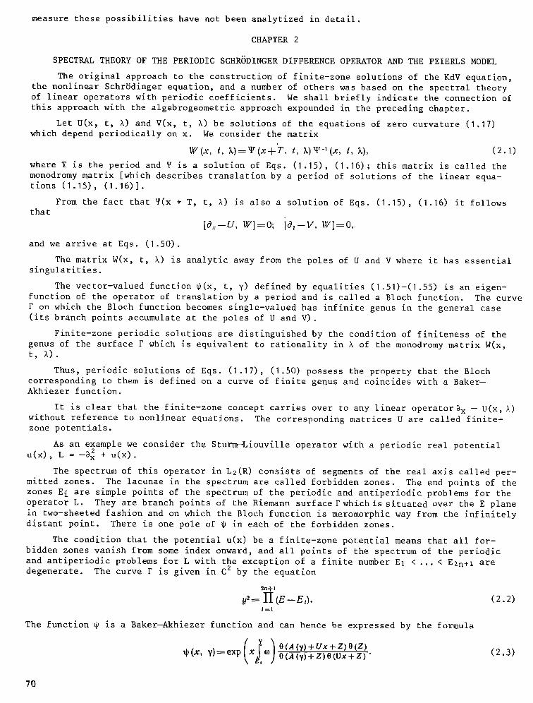
SPECTRAL THEORY OF THE PERIODIC SCHRODINGER DIFFERENCE OPERATOR AND THE PEIERLS MODEL

The original approach to the construction of finite-zone solutions of the KdV equation, the nonlinear SchrSdinger equation, and a number of others was based on the spectral theory of linear operators with periodic coefficients. We shall briefly indicate the connection of this approach with the algebrogeometric approach expounded in the preceding chapter.

Let U(x, t, ~) and V(x, t, ~) be solutions of the equations of zero curvature (1.17) which depend periodically on x. We consider the matrix

W(x, t, L ) = V ( x - ~ - T , t, k) V - ' ( x , t, ~), ( 2 . 1 )

where T i s t h e p e r i o d and ~ i s a s o l u t i o n of Eqs . ( 1 . 1 5 ) , ( 1 . 1 6 ) ; t h i s m a t r i x i s c a l l e d t he monodromy m a t r i x [wh ich d e s c r i b e s t r a n s l a t i o n by a p e r i o d of s o l u t i o n s of t h e l i n e a r e q u a - t i o n s ( 1 . 1 5 ) , ( 1 . 1 6 ) ] .

From t h e f a c t t h a t ~ (x + T, t , ~) i s a l s o a s o l u t i o n o f Eqs . ( 1 . 1 5 ) , ( 1 . 1 6 ) i t f o l l o w s t h a t

fox-v, Wl=0; io,-v, I 1=0,

and we a r r i v e a t Eqs . ( 1 . 5 0 ) .

The m a t r i x W(x, t , X) i s a n a l y t i c away f r o m t h e p o l e s of U and V where i t h a s e s s e n t i a l s i n g u l a r i t i e s .

The v e c t o r - v a l u e d f u n c t i o n ~ ( x , t , y) d e f i n e d by e q u a l i t i e s ( 1 . 5 1 ) - ( 1 . 5 5 ) i s an e i g e n - f u n c t i o n of t h e o p e r a t o r o f t r a n s l a t i o n by a p e r i o d and i s c a l l e d a B loch f u n c t i o n . The c u r v e F on which t h e B loch f u n c t i o n becomes s i n g l e - v a l u e d h a s i n f i n i t e genus i n t h e g e n e r a l c a s e ( i t s b r a n c h p o i n t s a c c u m u l a t e a t t h e p o l e s of U and V).

F i n i t e - z o n e p e r i o d i c s o l u t i o n s a r e d i s t i n g u i s h e d by t h e c o n d i t i o n of f i n i t e n e s s o f t h e genus of t h e s u r f a c e F which i s e q u i v a l e n t t o r a t i o n a l i t y in ~ of t h e monodromy m a t r i x W(x, t, ~ ) .

Thus, periodic solutions of Eqs. (1.17), (1.50) possess the property that the Bloch corresponding to them is defined on a curve of finite genus and coincides with a Baker-- Akhiezer function.

It is clear that the finite-zone concept carries over to any linear operator~ x -- U(x, %) without reference to nonlinear equations. The corresponding matrices U are called finite- zone potentials.

As an example we consider the Sturm--Liouville operator with a periodic real potential 2

u(x), L =--3x + u(x).

The spectrum of this operator in L2(R) consists of segments of the real axis called permitted zones. The lacunae in the spectrum are called forbidden zones. The end points of the zones E i are simple points of the spectrum of the periodic and antiperiodic problems for the operator L. They are branch points of the Riemann surface Fwhichis situated over the E plane in two-sheeted fashion and on which the Bloch function is meromorphic way from the infinitely distant point. There is one pole of ~ in each of the forbidden zones.

The condition that the potential u(x) be a finite-zone potential means that all forbidden zones vanish from some index onward, and all points of the spectrum of the periodic and antiperiodic problems for L with the exception of a finite number El < ... < E2n+l are degenerate. The curve F is given in C 2 by the equation

2n+l

y2--_ II (E--El). ( 2 . 2 ) /=1

The f u n c t i o n r i s a B a k e r - - A k h i e z e r f u n c t i o n and can h e n c e b e e x p r e s s e d by t h e f o r m u l a

( ~ )O(A(,)+Ux+Z)O(Z) ~(X, y ) = e x p x ~ O(A(y)+Z)O(Ux+Z) ( 2 . 3 )

70

Exanding (2.3) in a neighborhood of infinity, we obtain a formula [23] for finite-zone potentials of the Sturm-Liouville operator

0, u ( x ) = - - 2 ~ I n 0 ( U x + Z ) + const. (2 .4 )

An exposition of these results and of the spectral theory of finite-zone Sturm-Liouville operators globally can be found in [17].

I. Periodic Schr~dinger Difference Operator

The method of the inverse problem is applicable not only to partial differential equations but also to some differential-difference systems. For example, the equations of the Toda lattice [69]

X n = e -xn+xn+' - - e - x n - I +% ( 2 . 5 )

admit the Lax r e p r e s e n t a t i o n I~ = [A, L] , where

L*n -~- c.*n+t -t- ~On*n -~- ca-l*n-t , (2.6) A . I * Cll 41, Cr l - I Vn =-~- vn+,--T ~,-l, (2.7)

Vn = Xn, c2 = eXn+l-Xn- This representation was found in [38, 58].

An important difference of such systems from continuous systems is that all periodic solutions of differential-difference equations admitting representations of Lax type or of the more general difference analogue of the equations of zero curvature are finite-zone solutions.

Explicit expressions for periodic solutions of the equations of the Toda lattice were obtained in [33] (see also the author's appendix to [13]).

The purpose of the present section is an exposition of the algebrogeometric approach to the spectral theory of periodic difference operators for the example of the SchrSdinger difference operator (2.6). As already mentioned in the introduction, this theory plays an essential role not only in the construction of solutions of differential-difference systems but also in investigations of the Peierls model.

We consider operator (2.6) with periodic coefficients c n = Cn+N, Vn+ N = v n.

The basis of the modern approach to spectral problems for periodic operators is the investigation of the analytic properties of solutions of the equation

L ~ = E , . (2 .8 )

f o r a l l v a l u e s of the pa rame te r E i n c l u d i n g complex v a l u e s .

For any E the space of solutions of Eq. (2.8) is two-dimensional. Having given arbitrary values 0?0 and ~bl, all the remaining values ~0n are found from (2.8) in recurrent fashion. The standard basis ~n(E) and 0n(E) is given by the conditions (pa=1, (ps=0, 00=0, 01==I . From the recurrent procedure for computing ~n(E) and 0n(E) it follows that they are polynomials in E,

\ \ t = 2 /

' + ! . . . . (2.9) " ' " /

The matrix T(E) of the monodromy operator T:Yn § Yn+N in the basis ~p and 0 has the form

I (2.10) \q~,+~(E), ON+~(E)]"

From (2.8) it follows easily that for any two solutions of this equation, in particular, for r and 0, the expression (the analogue of the Wronskian)

c~ (~n0,,+t-- ~.+t0.)

71

does not depend on n. Since co = c N, it follows that

det T=~.VON+I--ON~N+I=~O01--~IO0 = | .

The eigenvalues w of the monodromy operator are found from the characteristic equation

I .2__ 2Q (E)* + 1 = 0; Q (E) = ~- (~.v (E) + 0.v+, (E)). (2.11)

The polynomial Q has degree N, and its leading terms have the form

1 / / ' v _ , \ �9 { "v-1 ,v -x ,~ ,~ 2Q(E) - . | E ' v - - | ~ k | e - v - ! + 1 ~ "ofo,,-- x ck~]E'v-2+ . . . . (2.12) )

The s p e c t r a E + o f t h e p e r i o d i c and a n t i p e r i o d i c p r o b l e m s f o r L a r e d e t e r m i n e d f r o m the e q u a t i o n Q(E~) = +1, s i n c e in t h i s c a s e w = + l .

We d e n o t e by E l , i = I , . . . , 2 q + 2, q ~< N -- I t he s i m p l e p o i n t s of t h e s p e c t r u m o f t h e p e r i o d i c and a n t i p e r i o d i c p r o b l e m s f o r L, i . e . , t h e s i m p l e r o o t s o f t h e e q u a t i o n

Q2(E)= I. ( 2 . 1 3 )

For a p o i n t E of g e n e r a l p o s i t i o n Eq. ( 2 . 1 1 ) h a s two r o o t s w and w - 1 . To e a c h r o o t t h e r e c o r r e s p o n d s a u n i q u e e i g e n v e c t o r {~n} o f t h e monodromy m a t r i x n o r m a l i z e d by the c o n - d i t i o n ~o = 1,

L~p. =Eq~. , ~,+.v = ~,.

This solution is called a Bloch solution. +

THEOREM 2. I. The two-valued function ~n(E) is a single-valued meromorphic function ~n(Y) on the hyperelliptic curve F, ~F, corresponding to the Riemann surface of the function v/R-(E) ',

2q+2

R (E)---- H (E--E,). (2.14) l=I

Away from the infinitely distant points it has q poles u infinitely distant points

In a neighborhood of the

(2.15)

Here the signs + correspond to the upper and lower sheets of the surface F (the upper sheet is the one on which at infinity /R ~ Eq+-l-).

The proof of this theorem repeats to considerable extent the analogous assertions from Sturm--Liouville theory [ 17] .

The Bloch solution, just as any other solution of Eq. (2.8), has the form ~,=~0~,+~t0,.

w--~ N The vector (~0, 41) is an eigenvector for the matrix T. Hence, ~0=I, ~t= 0, v or

~. = ~. (E) -} "-~.v 0 . v 0. (E). ( 2.1 6)

Suppose that ej, j = I .... ,N- q- i, are twofold roots of the equation Q2(E) = I, i.e.,

N--q--1

Q~(E) - - ] = C2r 2 (E) R (E), r (E) = H (E - - e j), ]=1

C-Z ~ C o ... C.,v,_ 1.

At the points ej in the Bloch basis the matrix of the operator T is equal to +I. it is equal to +I in any other basis. Thus,

(2.17)

Hence,

�9 e.v (E) = r (e)%.v (e), ~.v+, (E) = r (E)%.v§ (E),

~.v (e j)= e.v+1 (e j)= w (e j) = + I. (2.18)

(2.19)

72

From (2.19) it follows that Q(E)-~NCE)=rCE)Q(E).

Here ON, ~N+I, Q are polynomials in E. Substituting into (2.16) w = Q + CrY-and using the preceding equalities, we obtain

~ = ~. (E) ~ 0 (E)_=+_ C FR (Ei 0. (E). (2 .20) O N (E)

+ T h i s e q u a l i t y means t h a t t h e t w o - v a l u e d f u n c t i o n 0 ~ ( E ) i s a s i n g l e - v a l u e d , m e r o m o r p h i c

f u n c t i o n o f t h e p o i n t ~ F . The p o l e s o f 0 l i e a t t h e p o i n t s Y 1 , . . . , Y q e a c h o v e r a r o o t o f t h e p o l y n o m i a l 0N(E) . I n d e e d , i f 0N(E) = O, t h e n t h e two r o o t s Wl,2 a r e e q u a l t o ~N(E) and 0N+I (E) . Here ~,~(E)4=0N+I(E) . Hence , f o r one o f t h e r o o t s w [ i . e . , on one o f t h e s h e e t s o f F o v e r t h e r o o t 0H(E ) = 0J t h e n u m e r a t o r o f t h e f r a c t i o n i n ( 2 . 2 0 ) v a n i s h e s . The p o l e o f 0n l i e s on t h e s e c o n d s h e e t .

To c o m p l e t e t h e p r o o f i t r e m a i n s to c o n s i d e r t h e b e h a v i o r of 0~(E) as E § ~ . From ( 2 . 1 6 ) i t f o l l o w s t h a t a t P+01(E) has a s i m p l e p o l e . We f i n d d i r e c t l y f rom ( 2 . 8 ) t h a t 0n has a p o l e a t P+ of n - t h o r d e r , n > 0. S i m i l a r l y , 0 - n ( E ) h a s a p o l e a t P - o f n - t h o r d e r . From t h i s and t h e f a c t t h a t w h a s a t P+ a p o l e o f N - t h o r d e r w h i l e a t P - i t ha s a z e r o o f m u l t i p l i c i t y N we o b t a i n e q u a l i t y ( 2 . 1 5 ) where Xn a r e such t h a t x0 = 0, exp (x n -- Xn+l) = Cn.

The p a r a m e t e r s T 1 , . . . , Y q o r , more p r e c i s e l y , t h e i r p r o j e c t i o n s o n t o t h e E p l a n e (wh ich we h e n c e f o r t h d e n o t e i n t h e same way f o r b r e v i t y ) have a n a t u r a l s p e c t r a l m e a n i n g .

LEMMA 2 . 1 . The c o l l e c t i o n o f p o i n t s e j ( t w o f o l d d e g e n e r a t e p o i n t s o f t h e s p e c t r u m o f t h e p e r i o d i c and a n t i p e r i o d i c p r o b l e m s f o r L) and Y 1 , . . . , Y q fo rms t h e s p e c t r u m of p r o b l e m ( 2 . 8 ) w i t h z e r o b o u n d a r y c o n d i t i o n s ~0 = ~N = 0.

P r o o f . The c u r v e F o v e r t h e p o i n t s e j ha s two s h e e t s on each o f which t h e f u n c t i o n w(E) a s sumes t h e same v a l u e 1 o r --1. F o r ~n i t i s p o s s i b l e t o t a k e

~n (e j) = ~n ~ (el) - - ~n- (e]) = O~N (e j) O. (e l). ( 2.21 )

From (2.18) and the fact that r(ej) = 0 we find that ~0(ej) = ~N(ej) = 0.

The points Yi are the zeros of 0N(E). As already mentioned above, for E = Yi and for one of the signs in front of #R in (2.20) the numerator of the second term vanishes. Hence for the second it is nonzero. Suppose, for example, this is a plus sign. Then

is a nontrivial solution of Eq. (2.8), E = yj, with zero boundary conditions.

We consider the inverse problem. Suppose there are given arbitrary distinct points Ei, i = I,...,2q + 2 and points Y1,...,Yq on the Riemann surface F of the function ~-(E) whose projections onto the E plane are distinct. In difference problems the analogue of Theorem 1.5 is the Riemann--Roch theorem [44]. In the present case it asserts that there exists a meromorphic function 0n(Y) on F which is unique up to proportionality and has poles at the points YI,..-,Yq, a pole of n-th order at P+, and a zero of n-th order at the point P-. The function 0n(T) can be normalized up to sign by requiring that the coefficients of E • on the upper and lower sheets at infinity be mutual inverses. Fixing the sign in arbitrary fashion, we denote the corresponding coefficients by e • Here 0n(Y) will have the form (2.15) in a neighborhood of infinity.

LEMMA 2.2. The function 0n(Y) constructed satisfy Eq. (2.8) where the coefficients of the operator L are

c. = exp (x. - -x .+ , ) , ~.---- ~,+ (n) - - ~+ (n + 1). ( 2 . 2 2 )

P r o o f . We c o n s i d e r t h e f u n c t i o n ~ = L $ . - - E ~ . . I t h a s p o l e s a t t h e p o i n t s Y 1 , . . . , Y q . It follows from (2.15), (1.22) that ~, has a pole of order n -- I at P+ and a zero of order n at the point P-. By the Riemann--Roch theorem ~n=0.

The method of obtaining explicit formulas for On and the coefficients of L is completely analogous to the continuous case which was treated in the first chapter. As before, on F we fix a canonical collection of cycles. We denote by dp the normalized Abelian differential of third kind with sole singularities at infinity

73

q

l~q + E =lEq-I ~=t d E P ( B ) aB

i a p = V - ~ (e ) = y F - ( - E ) " (2.23)

The coefficients ai are determined from the normalization conditions

E2/+!

al ~'21 (2.24)

LEMMA 2.3. The function ~n(Y) has the form

*n=rnexp( itt i - / ap] O(A(~,)+Z(D)) ' (2.25)

where 27dUk=~dp, and r n is a constant. b k

In a neighborhood of the infinitely distant point on the upper sheet we have

exp i dp =Ee- lo( l - - l~E-~+. . . ) . (2 .26 )

It follows from (2.15) that exp(2x n + 210n) is equal to the ratio of the values of the factors of the exponential function in (2.25) taken at the images A(P +) = +z ~ From (2.25) and the fact that according to the Riemann bilinear relations 2z ~ = --IJ we obtain

c n 2 _ e _ 2 ~ * 0 (U (n--l) + Z) 0 ((n + I) U + Z) - - " 0' (nU+Z) ' (2.27)

where Z = Z(D) -- z ~

In a n e i g h b o r h o o d o f P+ we have

A (V) = z0 + VE-' + O (E-D,

where the coordinates V k of the vector V are determined by the equality

f~k=dE II (Vk + 0 (E-I).

Expanding (2 .25 ) in a s e r i e s in E - 1 , we o b t a i n f rom (2 .22 )

d ((n--1)U+Z+Vt) [ v n = a 7 I n 0 0 ( n U + Z + V t ) t=0 + I 1 "

(2.28)

THEOREM 2.2. Formulas (2.27), (1.28) recover the coefficients of L on the basis of the parameters E i and yj.

It is important to note that in general the formulas (2.27), (1.28) determine quasi- eriodic functions c n and v n. In order that c n and v n be periodic it is necessary and sufficient that for the corresponding differential dp the following conditions be satisfied:

U ~ = 2 ~ ms dp=-~-, mt--mtegers. ( 2 .29 ) b k

I t f o l l o w s f rom the d e f i n i t i o n of qn t h a t the p a r a m e t e r s E i , yj d e t e r m i n e them up to s i g n . Change of the s i g n s of {$n} l e a d s o n l y to a c o r r e s p o n d i n g change of the s i g n s of {Cn}. I t i s p o s s i b l e to no t d i s t i n g u i s h o p e r a t o r s d i f f e r i n g o n l y by the s i g n s o f the Cn, s i n c e t h e i r e i g e n f u n c t i o n s go ove r i n t o one a n o t h e r t r i v i a l l y . [Formula (2 .27 ) i s c o n s i s t e n t w i t h t he remain made above , s i n c e i t e x p r e s s e s in te rms of E i and yj n o t c n t h e m s e l v e s bu t t h e i r squares.]

Until now we have considered operators L with arbitrary complex coefficients. Suppose now that Vn and c n are real; then all the polynomials 0n(E), ~n(E), Q(E) introduced above are also real. Moreover, the periodic and antiperiodic problems for L are self-adjoint. This means that there are N real points of the spectrum of each problem, i.e., the polynomial Q2 _ | has 2N real roots. Hence at the extrema of the polynomial Q(E), dQ(E) = 0 we have IQ(E)[ I.

74

The segments [Eii- I, Eii] on which [Q(E) I ~ I are called permitted zones. In these segments lwl = I and the multivalued function p(E) defined from the equality w = tiP N is real. It is called the quasimomentum. Its differential coincides with (2.23) where in (2.24) a i are cycles situated over the forbidden zones [Eii, Eii+I]-

LEMMA 2.4. The poles Yi of the Bloch function ~n(u of a real operator L are situated such that there is one in each of the finite forbidden zones, Eii ~ Yi ~ Eii+l.

Proof. The poles Yi are zeros of the polynomial eN(E). At these points

1 = d e t T = ~N (~j) ON+l (Yj) ~- 1 .~

Since ~N and eN+ I are real, it follows that

and y] lies either in a forbidden zone or in one of the collapsed zones -- the points ej. In the letter it was shown above that @n(y) has no singularities. We consider the family of operators L t with coefficients c~ = t + (I -- t)c n, v~ = (I -- t)vn. It may be assumed with no loss of generality that c n > 0, since this can be achieved by changing the signs of c n which has no effect on Ei, yj. Since c~ = 0, it follows that y~, which depend continuously

i on t (just as E~), lie in forbidden zones for all t. For t = I all forbldden zones close up, i.e., all roots of the polynomial Q2 _ 1 except the first and last are twofold degenerate. Hence, y~ lie at two fold roots of Q2 _ 1. Deformation with respect to t leads to the situation that part of the twofold roots decompose into pairs of simple roots which are end points of a forbidden zone. Inside each of them there lies one point Yi by the continuity in t. For t = 0 we obtain the required assertion.

THEOREM 2.3. If the points EI,...,Eiq+ 2 are real and there is one of the points YI,..., yq of the corresponding Riemann surface over each of the forbidden zones [Eii, Eii+l], then the coefficients c n and v n of the operator L determined by them by Theorem 2.2 are real.

Proof. The necessity of the conditions of the theorem in the class of periodic operators is given by Lemma 2.4.

Suppose that the E~are real. Complex conjugation induces an antiinvolution �9 of the curve F:(E, /R-) § (E, CR). The fixed ovals of this antiinvolution are cycles situated over the segments [Eii, Eii+ I] and over the infinite zone joining the points Eiq+2, El through infinity.

We consider ~n(~(u This function posesses all the analytic properties of ~n- Since ~n is determined by these properties up to sign, it follows that

�9 n (* (?)) = • *n (?)- ( 2 . 3 0 )

It follows from (2.22) that the Vn are real, while the c n are either real or pure imaginary 2 is real) (i.e., c n

We shall prove that under the assumptions of the theorem c n = 0, c n = ~. The negation of this assertion is equivalent to the fact that one or several of the zeros Yi(n) of the function ~n(Y) is at infinity on the upper or lower sheet of F. From (2.30) it follows that on cycles situated over [Eii, Eii+l], ~nis either real or pure imaginary. On each cycle there is one pole Yi; therefore, there is at least one zero. Since there is a total of q zeros, it follows that Yi(n), like Yi, are situated one over each [Eii, Eii+l] and are hence bounded away from infinity.

By what has been proved, the sign of c~ does not change under continuous deformation of Ei and Yi for which the conditions of the theorem are satisfied. We deform them so that all the forbidden zones close. Here it is easy to verify that the operator L deforms into an operator L0 for which Vn = 0 and c~ = const > 0. The proof of the theorem is complete.

To conclude the section we consider conditions distinguishing operators L for which

v n = 0, i.e.,

L~n -~- Cn~n+l 2r- Cn-l~n-1. ( 2.31 )

Connected with this operator is the problem of integrating the difference analogue of

the KdV equation

Cnl:Cn ~(clz+l-c~-t), Cn ~ = c n 2" ( 2 . 3 2 )

75

THEOREM 2.4. The necessary and sufficient conditions that the operator L (constructed by Theorem 2.2 on the basis of the data E i and yj) has the form (2.31), i.e., v n = O, is the sy~m~etry of the points E i relative to zero and the invariance of the points yj relative to the involution on F

q+z

(e, ,," I ~ 1

Necessity of the conditions of the theorem follows from the fact that if ~n(T) is the Bloch function for the operator L of (2.31), then for ~n = (--1)n~n

Sufficiency of the conditions is proved in analogy to the proof of Theorem 2.3.

2. "Finite-Zone Potentials" and Variations of Kruskal's Integrals

As mentioned above, periodic operators are all finite-zone operators. Here the number of zones in the general case has the order of the period N of the operator. Distinguishing q-zone difference operators q < N can be carried out with the help of the same algebraic Ansatz as in the continuous case. Thus, for the SchrSdinger difference operator considered this Ansatz has the form: the operator L is a q-zone operator if and only if there is an operator

q+1

Lx~n= ~.~ dn, l,~n+k ( 2 . 3 3 ) km--q--1

such that

[L~, L]=0 . (2.34)

As in the continuous case, Eqs. (2.34) constitute essentially a pencil of nonlinear equations for the coefficients v n and c n of the operator L.

All solutions of these equations are given by formulas (2.27), (1.28) and are in general quasiperiodic functions of n.

The purpose of the present section is to present for this example still another aspect of the theory of finite-zone integration -- its connection with variational principles for functionals of Kruskal type.

We define functionals Ik = Ik{Cn, v n} by the formula

e~a

ip =- In E ~ ~ IkE -k, 4=0

where p(E) is the quasimomentum. These functionals have the form

N--!

n ~ 0

(2.35)

where the local densities r k are polynomials. From (2.12) we have

N--I I

Io = ~-" ~ In c,,, n ~ O

I Ii = "~" ~] "o,,

N - - 1

i 1 ~ / 2--vn*\ '=N--~0 to" + Y ) etc.

THEOREM 2.5. The operator L is a q-zone operator if and only if its coefficients are q+1

extremals of the functional f-f-----lq+2-~=jk, where ~k are certain constants. k=0

76

Because of this theorem, Eqs. (2.34) give a commutation representation of the pencil of equa t ions

q-F1 6H.=6fq.,=F~o~,,,SIk=0; 6=~(~C"SCnq=a~n6~n)n (2.36)

parametrized by the constants ek-

Proof. We shall first prove necessity of the conditions of the theorem.

LEMMA 2.5. There is the equality

/,Eq+'+/,Eq+... +/r l~=l~(SCn, 8Vn). (2.37) iSp = V R (e)

The proof of this relation can be obtained in complete analogy to the proof of its continuous variant [15].

We shall derive it from other considerations "which generalize easily to the case of variations not preserving the group of periods." (For the meaning of the last assertion see below.)

We consider an arbitrary variation 6Cn, 6v n of the operator L in the class of operators with the same period N. Under such variation the spectrum of the operator L is perturbed so that the end points of the old zones E i are shifted (we denote them by E~) and the twofold polnts of the spectrun ej posslbly decompose into slmple polnts e~ (at t~e site of the ej new lacunae are formed).

The quasimomentum is a multivalued function on F which on passing about the b-cycles changes by a integral multiple of 2n/N. Hence 6p is a single-valued meromorphic function on F. From (2.23) it follows that 6dp has poles of second order at the points E i and possibly simple poles over the points ej. From the single-valuedness of 6p it follows that the residues of 6dp over ej are equal to zero. Hence, ~p has simple p~les at the end points of the zones, and, since it is odd, equality (2.37) holds.

Expanding equality (2.37) in a neighborhood of infinity, we obtain

lo=-8;o, l

At • s, \ (2.38)

k - - I

l~ = -- 61 # + ~ [3,k611. t=0

From the first q + I equalities the coefficients Z k are expressed in terms of 6Ik, k ~< q + I. Equating the coefficients of the expansion (2.37) and (2.35) for E-q -2, we obtain (2.36) where e k are symmetric polynomials in E i.

The necessity of the conditions of the theorem follows from the fact that according to formula (2.37) for q-zone operators the coefficients Z k are independent and hence the differentials 61k, k ~< q + 2 are independent.

Let M q be the manifold of ordered collections E1 < ... < E2q+2. The closure MN is a stratified manifold containing Mq(~JW N for all q ~< N. For any collection El,... ,E2q+2 formula (2.23) defines a differential dp, and hence by (2.35) functionals Ik = Ik({Ei}).

We now consider the variation of (EI,...,E2q+2) in ~N. Under such variation, in addition to the variation Ei, there appear new lacunae ej < e~, j = I .... ,N -- q.

LEMMA 2.6. Let 6U k be the variation of the group of periods, i.e.,

Then r E IkEq+* k k=0

i s p = at ] / R (t)

(2.39)

77

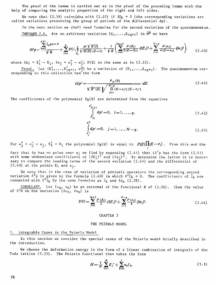
The proof of the lemma is carried out as in the proof of the preceding lemma with the help of comparing the analytic properties of the right and left sides.

We note that (2.39) coincides with (2.37) if 6U k = 0 (the corresponding variations are called variations preserving the group of periods of the differential dp).

In the next section we shall need formulas for the second variation of the quasimomentum.

THEOREM 2.6. For an arbitrary variation (EI,...,E2q+2) in ~N we have

q+l

i6,p_k=ov_g ' + 62U, ~ atVn(t) 4- p(e,) (6e,)2_~ Z 4(E--e,)(6ej)' t=x ai V ~ - - ~ (e-t) 2(E--El) /=, ' (2.40)

!

where 6Ei = E i -- E i, 6ej = e~ -- ej; P(E) is the same as in (2.23). v ; +

Proof. Let (EI,...,E2q+2 , e~) be a variation of (EI,...,E2q+2). r e s p o n d i n g t o t h i s c o l l e c t i o n h a s t h e f o r m

The quasimomentum cor-

PN (E) idp' = dE. /- N--q

I/~-57=~ l / IT (e--e~+) (e--ej-)

The coefficients of the polynomial PN(E) are determined from the equations

E'2i+!

dp'=O, i = 1 . . . . . q ,

1

~ dp t =O, j = l . . . . . N--q .

(2.41)

(2.42)

(2.43)

!

For e~ = ej = ej, E i = E i the polynomial PN(E) is equal to P(E)II(E--eI). From this and the I

fact that 6p has no poles over ej we find by expanding (2.41) that i62p has the form (2.41) with some undermined coefficients of (~Ei) 2 and (6ej) 2 To determine the latter it is necessary to compare the leading terms of the second varlation (2.41) and the differential of (2.40) at the points Ei and ej.

We note that in the case of variation of periodic operators the corresponding second variation ~2p is given by the formula (2.40) in which ~2U k = O. The coefficients of ~k are connected with 621k by the same formulas as I k and 61 k (2.28).

COROLLARY. Let (Cn, v n) be an extremal of the functional H of (2.36). Then the value of ~2H on the variation (6Cn, ~Vn) is

2q+2 N--q

62H= '~ ~P(E') (6E,)2_[ - ~.~ ~ (6el)=. (2.44) ~=i j=t

CHAPTER 3

THE PEIERLS MODEL

I. Integrable Cases in the Peierls Model

In this section we consider the special cases of the Peierls model briefly described in the introduction.

We choose the deformation energy in the form of a linear combination of integrals of the Toda lattice (2.35). The Peierls functional then takes the form

H = ~ - Ej+q-~• 1~1 k~O

(3.1)

78

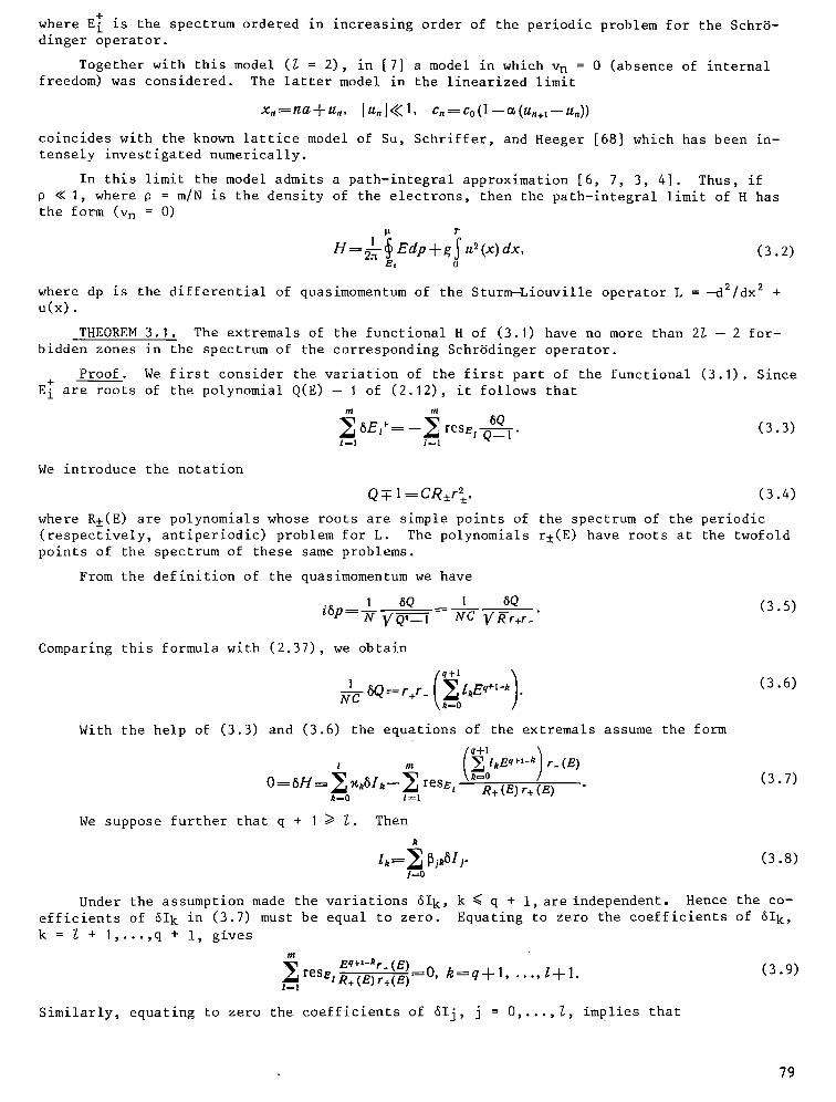
+ where E i is the spectrum ordered in increasing order of the periodic problem for the SchrS- dinger operator.

Together with this model (~ = 2), in [7] a model in which v n = 0 (absence of internal freedom) was considered. The latter model in the linearized limit

x~=naq-un, lu, l<<l, Cn=Co(I--O~(Un+l--Un) )

coincides with the known lattice model of Su, Schriffer, and Heeger [68] which has been in- tensely investigated numerically.

In this limit the model admits a path-integral approximation [6, 7, 3, 4]. Thus, if O << I, where p = m/N is the density of the electrons, then the path-integral limit of H has the form (v n = 0)

B T H = l ~ Edp+g ~ u2(x) ( 3 . 2 )

e t 0

where dp is the differential of quasimomentum of the Sturm--Liouville operator L = --d2/dx 2 + u(x).

THEOREM 3 . 1 . The e x t r e m a l s of t he f u n c t i o n a l H of ( 3 . 1 ) h a v e no more t han 22 -- 2 f o r - b i d d e n zones in t he s p e c t r u m o f the c o r r e s p o n d i n g S c h r ~ d i n g e r o p e r a t o r .

Proof. We first consider the variation of the first part of the functional (3.1). Since + E i are roots of the polynomial Q(E) -- I of (2.12), it follows that

m ~ 6Q

~-~6E~---- - - 'resetQ--I" (3 .3 ) 1=1 1~1

We introduce the notation

Q~ l=CR• (3.4)

where R• are polynomials whose roots are simple points of the spectrum of the periodic (respectively, antiperiodic) problem for L. The polynomials r• have roots at the twofold points of the spectrum of these same problems.

From the definition of the quasimomentum we have

6Q I 6Q (3.5) i6p~ N ~ Q~--I ~- N----C ~f Rr+r_"

Comparing this formula with (2.37), we obtain

/~+1 ) l 6Q_~_r+r_ik~=olkEq+l_ k (3.6)

NC

With the h e l p of ( 3 . 3 ) and ( 3 . 6 ) t h e e q u a t i o n s o f t h e e x t r e m a l s assume t h e f o r m

/ o+ t \ t m Ik~=olkE q+'-k) r_(E)

0= 6H= ~ Uk6Ik--~] rese, R+(E)r+(E) ( 3 . 7 ) 4 = 0 / = 1

We s u p p o s e f u r t h e r t h a t q + 1 /> ~. Then

k

I,= Z ~jk6lj. (3.81 ]=0

Under the assumption made the variations 61k, k ~ q + i, are independent. Hence the coefficients of 61 k in (3.7) must be equal to zero. Equating to zero the coefficients of 61k,

k = I + 1,...,q + i, gives

s Eq+l-~r-(E)--0, l - t ~R§ k = q + l . . . . . l + l . ( 3 . 9 )

Similarly, equating to zero the coefficients of ~lj, j = 0,...,l, implies that

79

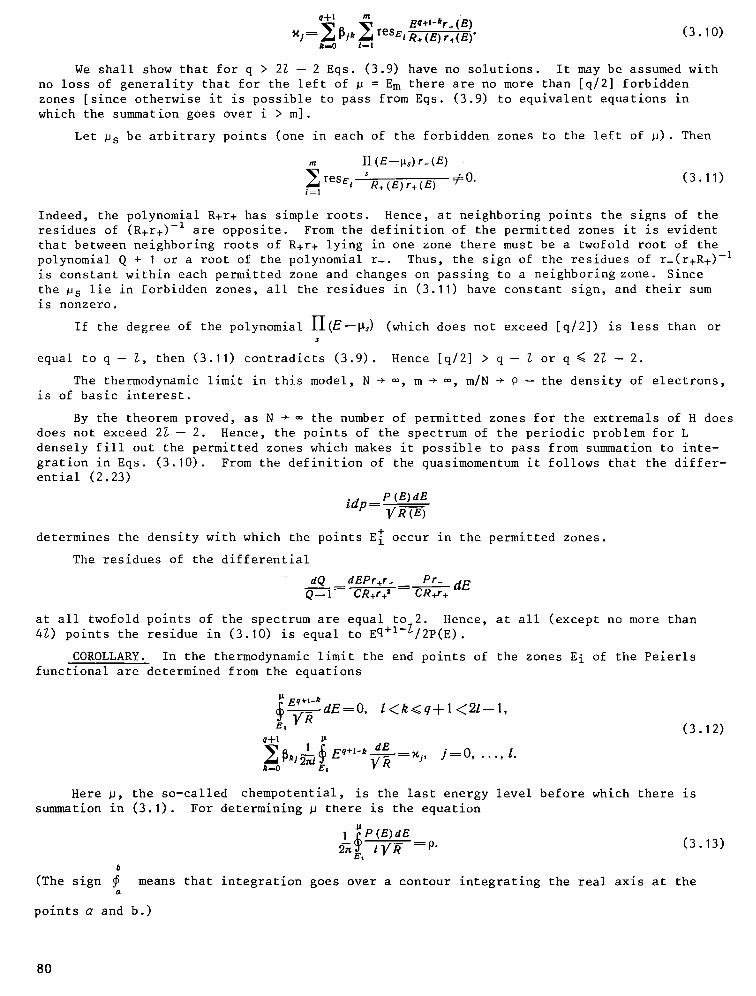
q+l ,. Bq+'-kr ~)"B" "1= ~ ~,k ~ rese, ~ ; . (3.10)

/z--O l--I

We shall show that for q > 2Z -- 2 Eqs. (3.9) have no solutions. It may be assumed with no loss of generality that for the left of ~ = E m there are no more than [q/2] forbidden zones [since otherwise it is possible to pass from Eqs. (3.9) to equivalent equations in which the summation goes over i > m].

Let ~s be arbitrary points (one in each of the forbidden zones to the left of ~). Then

II (P---~s) r_(E) resei R+(E)r+(E) =/=0. (3.1 1)

/=1

Indeed, the polynomial R+r+ has simple roots. Hence, at neighboring points the signs of the residues of (R+r+) -1 are opposite. From the definition of the permitted zones it is evident that between neighboring roots of R+r+ lying in one zone there must be a twofold root of the polynomial Q + I or a root of the polynomial r-. Thus, the sign of the residues of r_(r+R+) -1 is constant within each permitted zone and changes on passing to a neighboring zone. Since the Us lie in forbidden zones, all the residues in (3.11) have constant sign, and their sum is nonzero.

If the degree of the polynomial H(E--~s) (which does not exceed [q/2]) is less than or s

equal to q -- ~, then (3.11) contradicts (3.9). Hence [q/2] > q -- Z or q ~ 2Z - 2.

The thermodynamic limit in this model, N + ~, m + =, m/N + P -- the density of electrons, is of basic interest.

By the theorem proved, as N + = the number of permitted zones for the extremals of H does does not exceed 21 -- 2. Hence, the points of the spectrum of the periodic problem for L densely fill out the permitted zones which makes it possible to pass from summation to integration in Eqs. (3.10). From the definition of the quasimomentum it follows that the differential (2.23)

i d p _ = P ( E ) aE 1/~ (e)

+ determines the density with which the points E i occur in the permitted zones.

The residues of the differential

dO dEPr.r_ Pr_ d R ~ - - 1 = ~ = ~ - -

at all twofold points of the spectrum are equal to 2. Hence, at all (except no more than 4~) points the residue in (3.10) is equal to Eq+I-~/2P(E).

COROLLARY. In the thermodynamic limit the end points of the zones E i of the Peierls functional are determined from the equations

i Eq+'-k - 0 _-~-.__ d E = , l < k < q + l < 2 l 1,

q+l P

~0 1 E~ E q+l-' dE = ~k]~'~ ~ / ~ - = • j = 0 . . . . . l .

(3.12)

Here ~, the so-called chempotential, is the last energy level before which there is summation in (3.1). For determining ~ there is the equation

2-#~ i ~ R :P" (3.13) b

(The sign ~ means that integration goes over a contour integrating the real axis at the a

points a and b.)

80

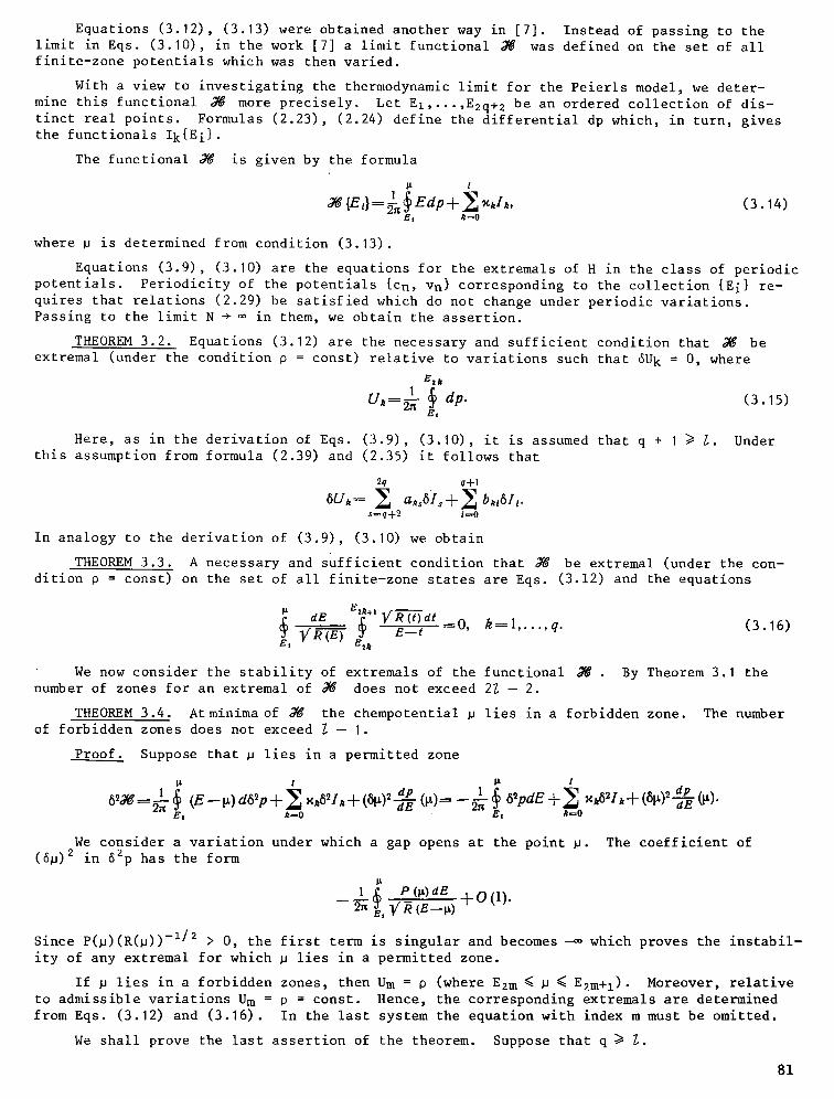
Equations (3.12), (3.13) were obtained another way in [7]. Instead of passing to the limit in Eqs. (3.10), in the work [7] a limit functional ~ was defined on the set of all finite-zone potentials which was then varied.

With a view to investigating the thermodynamic limit for the Peierls model, we determine this functional Jd more precisely. Let Ez,...,E2q+ 2 be an ordered collection of distinct real points. Formulas (2.23), (2.24) define the differential dp which, in turn, gives the functionals Ik{Ei}.

The functional ~ is given by the formula

Et /r (3.14)

where ~ is determined from condition (3.13).

Equations (3.9), (3.10) are the equations for the extremals of H in the class of periodic potentials. Periodicity of the potentials {Cn, Vn} corresponding to the collection {E i} re- quires that relations (2.29) be satisfied which do not change under periodic variations. Passing to the limit N § ~ in them, we obtain the assertion.

THEOREM 3.2. Equations (3.12) are the necessary and sufficient condition that ~ be extremal (under the condition O = const) relative to variations such that 6U k = 0, where

I Uk=~-~ ~ dp. (3.15) Et

Here, as in the derivation of Eqs. (3.9), (3.10), it is assumed that q + I ~ ~. Under this assumption from formula (2.39) and (2.35) it follows that

2q q + l

s ~ q + 2 t ~ 0

I n a n a l o g y t o t h e d e r i v a t i o n o f ( 3 . 9 ) , ( 3 . 1 0 ) we o b t a i n

THEOREM 3 . 3 . A n e c e s s a r y a n d s u f f i c i e n t c o n d i t i o n t h a t ~ b e e x t r e m a l ( u n d e r t h e c o n - d i t i o n 0 = c o n s t ) on t h e s e t o f a l l f i n i t e - z o n e s t a t e s a r e E q s . ( 3 . 1 2 ) and t h e e q u a t i o n s

Ea$+ I aE V R (t) dt ._=O, k = l . , q .

e , V~-T~T P - ~ " " E=k

(3.16)

We now consider the stability of extremals of the functional ~ . By Theorem 3.1 the number of zones for an extremal of ~ does not exceed 21 -- 2.

THEOREM 3.4. At minima of ~ the chempotential ~ lies in a forbidden zone. The number of forbidden zones does not exceed ~ -- I.

Proof. Suppose that ~ lies in a permitted zone

I 1 1 I 1 1

E , k=O E , k=O

We consider a variation under which a gap opens at the point ~. The coefficient of (~)2 in 62p has the form

1 ~ p (~)dE

Since P(~)(R(~)) -I/2 > 0, the first term is singular and becomes --= which proves the instabil- ity of any extremal for which ~ lies in a permitted zone.

If ~ lies in a forbidden zones, then Um = p (where E2m ~ ~ ~ E2m+l). Moreover, relative to admissible variations U m = O = const. Hence, the corresponding extremals are determined from Eqs. (3.12) and (3.16). In the last system the equation with index m must be omitted.

We shall prove the last assertion of the theorem. Suppose that q ~ I.

81

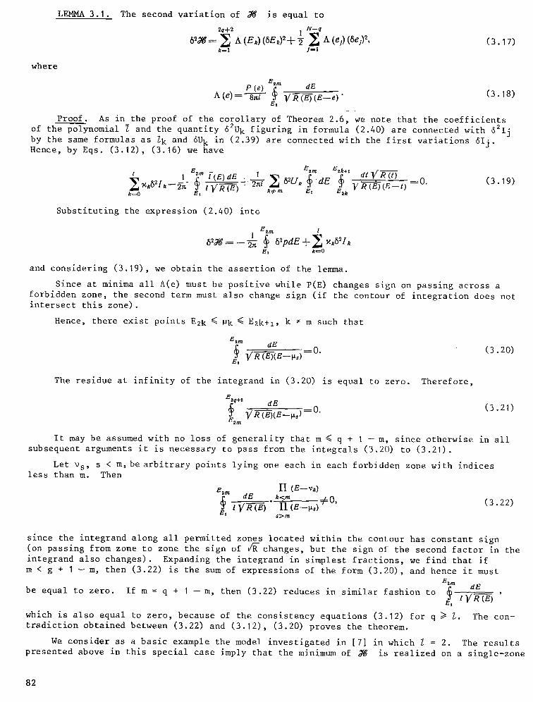
LEMMA 3 .1 .

where

The second variation of ~ is equal to

2q+2 1 N--q

k=l J--I (3.17)

~2 m P(e) de A(e)------~7-~l ~ ]/R(E)(E--e)" (3.18)

E,

Proof . As in the proof of the c o r o l l a r y of Theorem 2 .6 , we note t h a t the c o e f f i c i e n t s of the polynomial ~ and the q u a n t i t y 62Uk f i g u r i n g in formula (2.40) a re connected wi th ~2Ij by the same formulas as Z k and ~U k in (2.39) are connected wi th the f i r s t v a r i a t i o n s 6 I j . Hence, by Eqs. (3 .12 ) , (3.16) we have

-~0. (3.19)

Substituting the expression (2.40) into

E:~rn l 1 62~--__--~ ~ 6 2 p d E + ~ • 821.

Et k~0

and considering (3.19), we obtain the assertion of the lemma.

Since at minima all A(e) must be positive while P(E) changes sign on passing across a forbidden zone, the second term must also change sign (if the contour of integration does not intersect this zone).

Hence, there exist points E2k < ~k ~ E2k+l, k ~ m such that

E=m dE VR (e)(e--~) -0"

E,

(3.20)

The residue at infinity of the integrand in (3.20) is equal to zero. Therefore,

E~q§ (3.21 ) dE

V R ( e ) ( e - ~ ) = o. ~2m

It may be assumed with no loss of generality that m ~< q + I --m, since otherwise in all subsequent arguments it is necessary to pass from the integrals (3.20) to (3.21).

Let ~s, s < m, be arbitrary points lying one each in each forbidden zone with indices less than m. Then

e=,,, H (E--vk) dE ~<m ~0, (3.22)

:r ~ V R ~ } 11 {e - ) , , } Et s>m

since the integrand along all permitted zones located within the contour has constant sign (on passing from zone to zone the sign of ~changes, but the sign of the second factor in the integrand also changes). Expanding the integrand in simplest fractions, we find that if m < g + I -- m, then (3.22) is the sum of expressions of the form (3.20), and hence it must

Ezm

be equal to zero. If m = q + I -- m, then (3.22) reduces in similar fashion to iVR(E) E,

which is also equal to zero, because of the consistency equations (3.12) for q ~ I. The con- tradiction obtained between (3.22) and (3.12), (3.20) proves the theorem.

We consider as a basic example the model investigated in [7] in which I = 2. The results presented above in this special case imply that the minimum of ~Y~ is realized on a single-zone

82

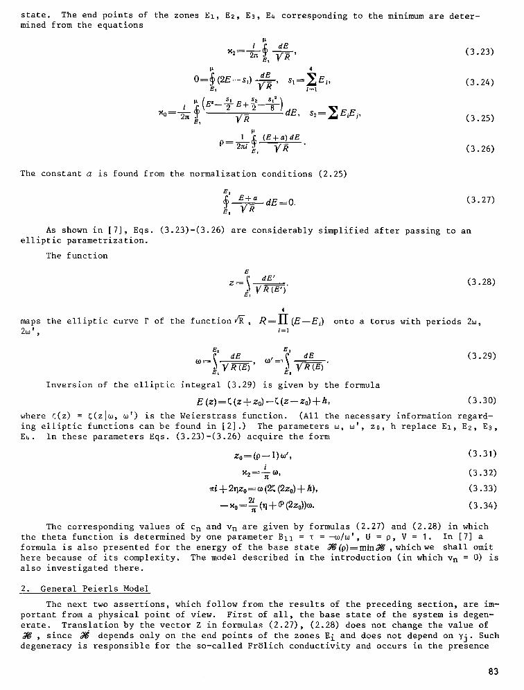
state. mined from the equations

The end points of the zones El, E2, E3, E4 corresponding to the minimum are deter-

~t l ~ dE

x2=-~- a , ~ , (3.23)

tt 4

0=~(2E--s,) ae e, ]/'R' SI=XEI'~=I (3.24)

, .~(e'--~ s, s , ' , e + ~ --if-)

x~ k, 1/R dE, s 2 = X E i E i, (3.25)

tl l__i_.~ (e+a)ae

P = 2hi ~, ]/ '~ (3.26)

The constant a is found from the normalization conditions (2.25)

E~ E+a

e, ]/ R dE =O. (3.27)

As shown in [7], Eqs. (3.23)-(3.26) are considerably simplified after passing to an elliptic parametrization.

The function

E I dE'

z = V ,~ (E')" E,

(3 .28)

4

maps the elliptic curve r of the function r R=H (E--Ei) onto a torus with periods 2m, 2~ ' ~=I

Ez E3

Et Et

Inversion of the elliptic integral (3.29) is given by the formula

E (z) = ~ (z q- Zo) -- ~ (z -- Zo) -4- h, ( 3 .30)

where ~(z) = ; ( z l ~ , ~ ' ) i s t h e W e i e r s t r a s s f u n c t i o n . (Al l the n e c e s s a r y i n f o r m a t i o n r e g a r d - ing e l l i p t i c f u n c t i o n s can be found in [ 2 ] . ) The p a r a m e t e r s ~, ~ ' , z0, h r e p l a c e E l , E2, E3, E~. In t h e s e p a r a m e t e r s Eqs. ( 3 . 2 3 ) - ( 3 . 2 6 ) a c q u i r e the form

Zo=(p__ l )~ , , (3 .31) i

• =-~ 00, (3.32)

~i --1- 2rlZo = o~ (2~ (gZo) + h), (3 .33)

-- xo = ~ (~i + ~ (2Zo))Co. (3 .34)

The corresponding values of c n and v n are given by formulas (2.27) and (2.28) in which the theta function is determined by one parameter BIt = T = -~/m', U = 0, V = I. In [7] a formula is also presented for the energy of the base state ~(p)=min~ , which we shall omit here because of its complexity. The model described in the introduction (in which v n = 0) is also investigated there.

2. General Peierls Model

The next two assertions, which follow from the results of the preceding section, are important from a physical point of view. First of all, the base state of the system is degenerate. Translation by the vector Z in formulas (2.27), (2.28) does not change the value of

, since ~ depends only on the end points of the zones E i and does not depend on yj. Such degeneracy is responsible for the so-called FrSlich conductivity and occurs in the presence

83

of additional sound (gapless) branches of the spectrum of excitations over the base state of the system. A second consequence is that ~(p) -- the energy of the base state -- is a smooth function of the density of electrons.

Below we shall consider the general Peierls model

1 ~ Edp+x212--• lYt

(3.35)

where

N--I

W = lira 1 ~ (~x (v,) + ~.~ (c,?)). ( 3 . 3 6)

It is found that in the general case the energy of the base state ~Y~.(P) for g = 0 becomes discontinuous at rational points p = r/q. The magnitude of the jump has order ~gexp (--aq). A number of physical considerations and results of machine computations [9, 50] indicate that degeneracy of the base state is also connected with questions of commensurability (to which a great deal of attention has recently been devoted in the physics literature (see, for example, the survey [51])). We shall prove that for irrational p and 0 ~< g ~< gp the base state is indeed degenerate.

Below the functional (3.35) with g = 0 (which was considered as the basic example in the preceding section) will be denoted by ~0.

We point out that in a neighborhood of the base state ~0 is not a smooth function, since in this state E 2 ~ ~ ~ E3. which

We denote by ~o(9, U)

The functional o'~o is smooth relative to variations for

Es

J- I dp=U=const. 2~ B,

(3.37)

the minimum of ~0 on the set of single-zone states for fixed p and U in (3.37). The end points of the zones corresponding to this minimum are determined from Eqs. (3.23)-(3.26). Here if U > p, then El ~ ~ < E2, while if U < p then E3 < ~ ~ E4.

The derivative a~0(U.@) is discontinuous at the point U = p. It follows from (2.39) that 0U

it has right and left limits h(Ea) > 0 and h(Ee) < 0, respectively, where

e E ,

k (e) = ~-fi~ e - - t t E l

(3.38)

Function h(e) decreases monotonically on the segments [Ez, E2] and [E3, E~]. Here h(El) = h(E4) = 0. On the segment [E2, E3] it increases linearly from h(E2) < 0 to h(E3) > 0. Hence, in a neighborhood of U = p.

~ o (U, O) = ~ o (0).+ k, l U - - 0 ] + k2 (U - - 9) + 0 ((U - - P)D, ( 3 . 3 8' ) & + h ~ = k (E~), h2--&=k(E2).

Remark. In the definition of the chempotential given above its value inside a forbidden zone was ambiguous. If we define ~ in this case by means of the relation

a~ (p)

~ = T '

then from (3.38) ~ will satisfy the equality h(~) = 0.

For small g the system (3.35) can be considered as a perturbation of the integrable model with g = 0. In order to apply considerations usual in such cases, in proving the main theorem of this section, we shall need formulas for the second variation of ~0 and for the first variation of W.

Substituting (2.27) and (2.28) into (3.36), it may be assumed that W is a function

W= W({&}, Z) of the collection {E i} = (E1,...,E2q+2), Z = (z1,...,Zq).

84

We consider the nature of the dependence of W on Z.

Formula (2.29) assigns to each collection {Ei} a q-dimensional vector U({Ei}) with coordinates 0 < U1 < ... < Uq < I. The collection {Ei} is called a nonresonance collection if there does not exist an integral vector r = (rl,...,rq) such that

< r, U({E~}) ) = t o , ( 3 .39 )

where r0 is an integer. For resonance collections R({Ei}) will denote the group formed by the same rQR({Ei}) for which (3.39) holds for some integer r0.

LEMMA 3.2. The functional W is equal to

W({E~, Z})= ~ ~',exp(2ni<r, Z > + n i r o ) , (3.40) ,E~({ed)

where

~ , , = I . . . I $: (z , . . . . . zq)e-2"~ <,", " > d z t . . . d z q

are the Fourier coefficients of the function

s" (z) = ~, (v (z)) + ~ (c 2 (z)), c~ = o(z--u)o(z+u) e_2,o, U = U ( { E i } ) ,

O'(Z)

v ( Z ) = a In O(Z+U) o(z+u+vt) t-o-- Ia.

(3.41)

(3.42)

From (2.27), (2.28) it follows that

*, (Vn) + @2 (c,2)= t~t" (nu--U-I- Z).

The limit

N--!

lira I E~(nU--U- t -ZI

is easily found by using the Fourier expansion for ~'(z).

COROLLARY I. For nonresonance collections {E i} W does not depend on Z and is equal to

Wo ({E,})= ! . . . I ~(Z)dzl . . .dze (3 .43 )

COROLLARY 2. If not all the frequencies Uk are rational, then the corresponding level of the functional W is degenerate.

Proof. Under the assumption of the corollary all the resonance relations are dependent. Hence, there is a vector Z, such that <r, Z,> = 0. It then follows from (3.40) that W({Ei}, Z + tZ,) does not depend on t.

Formula (3.43) defines the "continuous" part of the functional W which for general ~i and ~2 is discontinuous at all resonance collections. If Ir[ is the minimal order of resonance, ~rl----Irllq-...~.Irql, rER({EI}) , then the magnitude of the jump

IW ({E,}, Z)--Wo({E,})I

has order ~'r and decreases with increasing lrl for analytic 0i like exp (-alrl), where a is a constant.

We denote by W,({Ei})=minV/({Ei}, Z) By Corollary I it is equal to W0 almost everywhere. Z

It follows from (3.40) that

I " " l w ({E,}, z ) a z , . . , azq = Wo ({E,}).

Hence,

w , ({E,}) ~< Wo ({E,}).

85

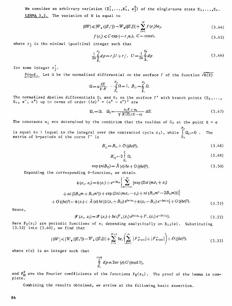
v v + We consider an arbitrary variation (EI,...,E~, e~) of the single-zone state EI,...,E4.

LENNA 3 . 3 . The v a r i a t i o n of W i s equa l to

N

[6UZl -.< Ire, ((E,'})-- VC,C{E,})[ + ~ / (ej)6e~, (3.44) j = l

f (e j) -.< C exp ( - - rf~t), C -- const, ( 3 .4 5)

where r j i s the minimai ( p o s i t i v e ) i n t e g e r such t h a t

dp=r,Uq-r/ , u = l ~dp E~ L~t

! f o r some i n t e g e r r j .

P r o o f .

(3.46)

Let ~ be the normalized differential on the surface F of the function

d E E~ E2 :, a.

E~ E

The normalized Abelian differentials ~i and ~2 on the surface F' with branch points (El,..., E4, e-, e +) up to terms of order (6e) 2 = (e +- e-) 2 are

a,E+a2 dE. (3 .47) fl,----.Q, f12= 1 /N(~)(E_e)

The constants ~i are determined by the condition that the residue of ~2 at the point E = e

Es

is equal to I (equal to the integral over the contracted cycle a2), while .I ~2-~-0 " The matrix of b-periods of the curve F' is ~,

B;, = B , , Jr 0 ((6&),

B12=2 i ~,

exp (niB2~) = A (e) 6eq- O ((6e)~).

Expanding the c o r r e s p o n d i n g 0 - f u n c t i o n , we o b t a i n

O(zl, z~)=O(zO+e "iB" ~ [exp(2r~i(mzt-t-z2)

-b ~i (2B,2m + BI ira2)) -6 exp (2ai (mzi- z2) + ai (B,lm 2 --2Bto_m))l}

Jr O ((6e) 2) = 0 (z0 q- A (e) 6e [0 (zl -t- B~2) e -'~t ~' -k 0 (z, - - B,~) e -2~i~,1 ~- O ((6&).

Hence,

(z,, z.~) = ~r (z0 + 6e (F+ (zl) e 2"t~' + F (z0 e-2"~').

Here F • a r e p e r i o d i c f u n c t i o n s of zz depend ing a n a l y t i c a l l y on B12(e ) . (3.52) into (3.40), we find that

[r,,r(e) I§ Ir~(e) l +O (0e)2), 16W/I~<IW,({EI'})--W,({E,})I~-Z fie, + i = l l

(3.48)

(3.49)

(3.50)

(3.51)

(3.52)

Substituting

(3.53)

where r(e) is an integer such that

r(e)

~. dp-- 2ar (e) U (rood 1), E,

and F~ are the Fourier coefficients of the functions Fi(zl). The proof of the lemma is complete.

Combining the results obtained, we arrive at the following basic assertion.

86

THEOREM 3.5. Suppose that r and r are analytic in some neighborhood of the real axis on which they are positive, and suppose that P satisfies the condition Ip --m/nl > a/n 2 for n > no, where no and a are some constants. Then there exists go > 0 such that for g < go the energy of the base state ~.(p)=min~ satisfies the inequality

g2C2 !g e , (0) - ~ , ({E,*}) I < 2A '

where E i i s t he b a s e s t a t e f o r t he u n p e r t u r b e d f u n c t i o n a l ~Y~0~ which i s g i v e n by ( 3 . 2 3 ) - ( 3 . 2 6 ) and h > 0 i s e q u a l to m i n h ( e ) in ( 3 . 1 8 ) .

Furthermore,

I. The spectrum of the operator L corresponding to the base state of the system has gaps at the points e s defined from the condition

e$ l__ 2n I d p ~ s p ( m o d l ) .

El

2. The width of the gap has order

16es ] < .gC exp (--sat) + 0 (gD. 2A

3. The b a s e s t a t e i s g i v e n by f o r m u l a s ( 2 . 2 7 ) and (2 .2 8 ) in which a l l f r e q u e n c i e s have t he fo rm

U, = rkp + rk', !

where rk , rk a r e i n t e g e r s .

4. I f p i s i r r a t i o n a l , t h e n the b a s e s t a t e i s d e g e n e r a t e .

Proof. We denote by V,c7~ a neighborhood of {E~} consisting of collections (E~, e~) such that

N - - , 4

1=I lft

denote by V h the complement of this neighborhood. and we

Because ~0 has no extremals besides {E~} and r and r are positive, for sufficiently small h we have

(3.54)

rain a~, > min ~0 > ~0 (P) + A h=" g ~h vh

I f gW. ({E,}) ~< A h'-' , then the minimum of

~ , (P) --< ge0 (P) + gW ({E,})

i s a c h i e v e d in t he n e i g h b o r h o o d V h.

Let P be as in the condition of the theorem; then W is differentiable at {E*} relative to all variations including those changing the period

E~

Indeed, if [U- 01 < E, U = m/n, then n > fa~/E.

Hence

E IW, ({e,})-w0 ({e,})l < c, exp(-- ~/f-g al)

and W({Ei}) has a derivative with respect to U equal to the derivative of W0.

87

Suppose that g satisfies the condition

OW ,~<min (h, + h2), guu EI=E I

w h e r e t h e h i a r e d e f i n e d i n ( 3 . 3 8 ' ) . From ( 3 . 3 8 ' ) i t t h e n f o l l o w s t h a t r n i n ~ i s a c h i e v e d for U = p.

Let (E;, e j) be the base state of the system. Since it belongs to Vh, it is possible to use the results of Lemmas 3.1 and 3.3. We have

g=6'= Ygo-~ gWmYgo(o)+A~2+gIV* ({Ei*})-gce >FNo(p)+gW*({E'*}) 2a '

where c i s d e f i n e d i n ( 3 . 5 4 ) . From t h e " d i a g o n a l i t y " of 6-~176 0 i t i s p o s s i b l e t o o b t a i n a more precise estimate for the width of each new gap

c f ( e ~ ) / f(e~) : Cexp(--r~a,) 6ej ~ 2A (e~) "~ g ~ ~'" g 2A

Thus, all parts of the theorem except the last have been proved. The degeneracy of the base state for irrational P is given by Corollary 2 of Lemma 3.2.

We note that the zone structure of the SchrSdinger difference operator corresponding to the base state of the Peierls model (which, by what has been proved, is quasiperiodic with the two periods 0 and I) is altogether analogous to the structure of the spectrum of the Sturm-Liouville operator with an almost periodic potential which was obtained in [56] (for application of the results of [56] in path-integral approximations in the Peirls problem see [51]).

LITERATURE CITED

I. N. I. Akhiezer, "A continual analogue of orthogonal polynomials on a system of inter- vals," Dokl. Akad. Nauk SSSR, 141, No. 2, 263-266 (1961).

2. H. Bateman and E. Erdelyi, Higher Transcendental Functions [in Russian], Nauka, Moscow (1974).

3. E. D. Belokolos, "The Peierls--Frolich problems and finite-zone potentials. 1 i, Teor Mat. Fiz., 45, No. 2, 268-280 (1980).

4. E. D. Belokolos, "The Peierls--FrSlich problems and finite-zone potentials. II," Teor. Mat. Fiz., 48, No. I, 60-69 (1981).

5. S. A. Brazovskii, S. A. Gordyunin, and N. N. Kirova, "Exact solution of the Peierls model with an arbitrary number of electrons on an elementary cell," Pis'ma Zh. Eksp. Teor. Fiz., 31, No. 8, 486-490 (1980).

6. S. A. Brazovskii, I. E. Dzyaloshinskii, and N. N. Kirova, "Spin states in the Peierls model and finite-zone potentials," Zh. Eksp. Teor. Fiz., 82, No. 6, 2279-2298 (1981).

7. S.A. Brazovskii, I. E. Dzyaloshinskii, and I. M. Krichever, "Exactly solvable discrete Peierls models," Zh. Eksp. Toer. Fiz., 83, No. I, 389-415 (1982).

8. I. M. Gel'fand and L. A. Dikii, "Asymptotics of the resolvent of Sturm--Liouville equations and the algebra of Korteweg--de Vries equations," Usp. Mat. Nauk, 30, No. 5, 67-100 (1975). I. E. Dzyaloshinskii, "Theory of helicoidal structures," Zh. Eksp. Teor. Fiz., 47, No. 5, 992-1008 (1964). I. E. Dzyaloshinskii and I. M. Krichever, "Effects of commensurability in the discrete Peierls model," Zh. Eksp. Teor. Fiz., 83, No. 5, 1576-1581 (1982). I. E. Dzyaloshinskii and I. M. Krichever, "Sound and the wave of charge density in the discrete Peierls model," Zh. Eksp. Teor. Fiz., 95 (1983). (in the press) B. A. Dubrovin, "The periodic problem for the Korteweg--de Vries equation in the class of finite-zone potentials," Funkts. Anal. Prilozhen., 9, No. 3, 41-51 (1975). B. A. Dubrovin, "Theta functions and nonlinear equations," Usp. Mat. Nauk, 36, No. 2, 11-80 (1981). B. A. Dubrovin, "The inverse problem of scattering theory for periodic finite-zone potentials," Funkts. Anal. Prilozhen., 9, No. I, 65-66 (1975). B. A. Dubrovin, V. B. Matveev, and S. P. Novikov, "Nonlinear equations of Korteweg--de Vries type, finite-zone linear operators, and Abelian manifolds," Usp. Mat. Nauk, 31, No. I, 55-136 (1976). B. A. Dubrovin and S. M. Natanzon, "Real two-zone solutions of the sine-Gordon equation," Funkts. Anal. Prilozhen., 16, No. I, 27-43 (1982).

.

10.

11.

12.

13.

14.

15.

16.

88

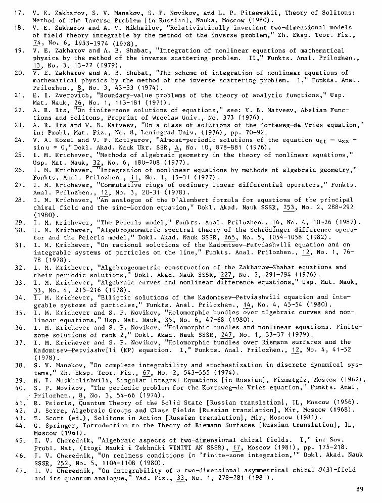
17. V. E. Zakharov, S. V. Manakov, S. P. Novikov, and L. P. Pitaevskii, Theory of Solitons: Method of the Inverse Problem [in Russian], Nauka, Moscow (1980).

18. V. E. Zakharov and A. V. Mikhailov, "Relativistically invariant two-dimensional models of field theory integrable by the method of the inverse problem," Zh. Eksp. Teor. Fiz., 7_44, No. 6, 1953-1974 (1978).

19. V. E. Zakharov and A. B. Shabat, "Integration of nonlinear equations of mathematical physics by the method of the inverse scattering problem. II," Funkts. Anal. Prilozhen., 13, No. 3, 13-22 (1979).

20. V. E. Zakharov and A. B. Shabat, "The scheme of integration of nonlinear equations of mathematical physics by the method of the inverse scattering problem. I," Funkts. Anal. Prilozhen., 8, No. 3, 43-53 (1974).

21. E. I. ZverovTch, "Boundary-value problems of the theory of analytic functions," Usp. Mat. Nauk, 26, No. I, 113-181 (1971).

22. A. R. Its, "On finite-zone solutions of equations," see: V. B. Matveev, Abelian Func- tions and Solitons, Preprint of Wroclaw Univ., No. 373 (1976).

23. A. R. Its and V. B. Matveev, "On a class of solutions of the Korteweg--de Vries equation," in: Probl. Mat. Fiz., No. 8, Leningrad Univ. (1976), pp. 70-92.

24. V. A. Kozel and V. P. Kotlyarov, "Almost-periodic solutions of the equation utt -- Uxx + sinu = 0," Dokl. Akad. Nauk Ukr. SSR, A, No. 10, 878-881 (1976).

25. I. M. Krichever, "Methods of algebraic geometry in the theory of nonlinear equations," Usp. Mat. Nauk, 32, No. 6, 180-208 (1977).

26. I. M. Krichever, "Integration of nonlinear equations by methods of algebraic geometry," Funkts. Anal. Prilozhen., 11, No. I, 15-31 (1977).

27. I. M. Krichever, "Commutative rings of ordinary linear differential operators," Funkts. Anal. Prilozhen., 12, No. 3, 20-31 (1978).

28. I. M. Krichever, "An analogue of the D'Alembert formula for equations of the principal chiral field and the sine-Gordon equation," Dokl. Akad. Nauk SSSR, 253, No. 2, 288-292 (1980).

29. I. M. Krichever, "The Peierls model," Funkts. Anal. Prilozhen., 16, No. 4, 10-26 (1982). 30. I. M. Krichever, "Algebrogeometric spectral theory of the Schr~dinger difference opera-

tor and the Peierls model," Dokl. Akad. Nauk SSSR, 265, No. 5, 1054-1058 (1982). 31. I. M. Krichever, "On rational solutions of the Kadomtsev--Petviashvili equation and on

integrable systems of particles on the line," Funkts. Anal. Prilozhen., 12, No. I, 76- 78 (1978).

32. I. M. Krichever, "Algebrogeometric construction of the Zakharov--Shabat equations and their periodic solutions," Dokl. Akad. Nauk SSSR, 227, No. 2, 291-294 (1976).

33. I. M. Krichever, "Algebraic curves and nonlinear difference equations," Usp. Mat. Nauk, 33, No. 4, 215-216 (1978).

34. I. M. Krichever, "Elliptic solutions of the Kadomtsev--Petviashvili equation and integrable systems of particles," Funkts. Anal. Prilozhen., 14, No. 4, 45-54 (1980).

35. I. M. Krichever and S. P. Novikov, "Holomorphic bundles over algebraic curves and nonlinear equations," Usp. Mat. Nauk, 35, No. 6, 47-68 (1980).

36. I. M. Krichever and S. P. Novikov, "Holomorphic bundles and nonlinear equations. Finite- zone solutions of rank 2," Dokl. Akad. Nauk SSSR, 247, No. I, 33-37 (1979).

37. I. M. Krichever and S. P. Novikov, "Holomorphic bundles over Riemann surfaces and the Kadomtsev--Petviashvili (KP) equation. I," Funkts. Anal. Prilozhen., 12, No. 4, 41-52 (1978).

38. S. V. Manakov, "On complete integrability and stochastization in discrete dynamical systems," Zh. Eksp. Teor. Fiz., 67, No. 2, 543-555 (1974).

39. N. I. Muskhelishvili, Singular Integral Equations [in Russian], Fizmatgiz, Moscow (1962). 40. S. P. Novikov, "The periodic problem for the Korteweg-de Vries equation," Funkts. Anal.

�9 Prilozhen., 8, No. 3, 54-66 (1974). 41. R. Peierls, Quantum Theory of the Solid State [Russian translation], IL, Moscow (1956). 42. J. Serre, Algebraic Groups and Class Fields [Russian translation], Mir, Moscow (1968). 43. E. Scott (ed.), Solitons in Action [Russian translation], Mir, Moscow (1981). 44. G. Springer, Introduction to the Theory of Riemann Surfaces [Russian translation], IL,

Moscow (1961). 45. I. V. Cherednik, "Algebraic aspects of two-dimensional chiral fields. I," in: Sov.

Probl. Mat. (Itogi Nauki i Tekhniki VlNITI AN SSSR), 17, Moscow (1981), pp. 175-218. 46. I. V. Cherednik, "On realness conditions in 'finite-zone integration,'" Dokl. Akad. Nauk

SSSR, 252, No. 5, 1104-1108 (1980). 47. I. V. Cherednik, "On integrability of a two-dimensional asymmetrical chiral #(3)-field

and its quantum analogue," Yad. Fiz., 33, No. I, 278-281 (1981).

89

48. I. V. Cherednik, "On solutions of algebraic type of asymmetric differential equations," Funkts. Anal. Prilozhen., 15, No. 3, 93-94 (1981).

49. M. A. Ablowitz, D. J. Kaup, A. S. Newell, and H. Segur, "Method for solving the sine- Gordon equation," Phys. Rev. Lett., 30, 1262-1264 (1973).

50. S. Aubry, " Analytlcity breaking and Anderson localization in incommensurate lattices," Ann. Israel Phys. Soc., ~, 133-164 (1980).

51. S. Aubry, "Metal--insulator transition in one-dimensional deformable lattices," Bifurca- tion Phenomena in Math. Phys. and Related Topics, C. Bardos and D. Bessis (eds.) (1980), pp. 163-184.

52. H. M. Baker, "Note on the foregoing paper 'Commutative ordinary differential operators,'" Proc. R. Soc. London, 118, 584-593 (1928).

53. R. K. Bullough and P. J. Caudrey (eds.), Solitons, Springer-Verlag (1980). 54. F. Calodgero, "Exactly solvable one-dimensional manybody systems," Lett. Nuovo Cimento,

13, 411-415 (1975). 55. D. V. Choodnovsky and G. V. Choodnovsky, "Pole expansions of nonlinear partial differ-

ential equations," Lett. Nuovo Cimento, 40B, 339-350 (1977). 56. E. I. Dinaburg and Y. C. Sinai, "Schr~dinger equation with quasiperiodic potentials,"

Fund. Anal., 9, 279-283 (1976). 57. L. D. Faddeev, Quantum Scattering Transformation, Proc. Freiburg Summer Inst., 1981,

Plenum Press (1982). 58. H.'Flaschka, "Toda lattice. II," Prog. Theor. Phys., 5__11, 543-555 (1974). 59. C. Gardner, J. Green, M. Kruskas, and R. Miura, "A method for solving the Korteweg--de

Vries equation," Phys. Rev. Lett., 19, 1095-1098 (1967). 60. P. D. Lax, "Integrals of nonlinear equations of evolution and solitary waves," Commun.

Pure Appl. Math., 21, No. 5, 467-490 (1968). 61. A. N. Leznov and M. N. Saveliev, "On the two-dimensional system of differential equa-

tions," Commun. Math. Phys., 74, 111-119 (1980). 62. P. Mansfild, "Solutions of the Toda lattice," Preprint Cambridge Univ., Cambridge, CB

39 EW (1982). 63. A. V. Mikhailov, "The reduction problem in the Zakharov--Shabat equations," Physica 3D,

i, 215-243 (1981). 64. A. V. Mikhailov, "The Landau--Lifshits equation and the Riemann--Hilbert bound@ry problem

on the torus," Phys. Lett., 92a, 2, 51-55 (1982). 65. A. M. Perelomov, "Completely integrable classical systems connected with semisimple Lie

algebras," Lett. Math. Phys., I, 531-540 (1977). 66. K. Pohlmeyer, "Integrable Hamiltonian systems and interaction through quadratic con-

straints," Commun. Math. Phys., 46, 207-223 (1976). 67. E. K. Sklyanin, "On complete integrability of the Landau--Lifshitz equation," Preprint

LOMI E-3-1979, Leningrad (1979). 68. W. P. Su, I. R. Schriffer, and A. I. Heeger, "Soliton excitations in polyacetylene,"

Phys. Rev., B22, 2099-2108 (1980). 69. M. Toda, "Waves in nonlinear lattices," Prog. Theor. Phys. Suppl., 45, 174-200 (1970).

90

Nonlinear equations and elliptic curves

Documents

Transcript of Nonlinear equations and elliptic curves