Nonlinear Control of Mechanical Systems With an Unactuated Cyclic Variable

IEEE TRANSACTIONS ON AUTOMATIC CONTROL, VOL. 50, NO. 5, MAY 2005 559

Nonlinear Control of Mechanical Systems With anUnactuated Cyclic Variable

J. W. Grizzle, Fellow, IEEE, Claude H. Moog, Senior Member, IEEE, and Christine Chevallereau

Abstract—Numerous robotic tasks associated with underactua-tion have been studied in the literature. For a large number ofthese in the plane, the mechanical models have a cyclic variable,the cyclic variable is unactuated, and all shape variables are inde-pendently actuated. This paper formulates and solves two controlproblems for this class of models. If the generalized momentumconjugate to the cyclic variable is not conserved, conditions arefound for the existence of a set of outputs that yields a system witha one-dimensional exponentially stable zero dynamics—i.e., an ex-ponentially minimum-phase system—along with a dynamic exten-sion that renders the system locally input-output decouplable. Ifthe generalized momentum conjugate to the cyclic variable is con-served, a reduced system is constructed and conditions are foundfor the existence of a set of outputs that yields an empty zero dy-namics, along with a dynamic extension that renders the systemfeedback linearizable. A common element in these two feedbackproblems is the construction of a scalar function of the configura-tion variables that has relative degree three with respect to one ofthe input components. The function arises by partially integratingthe conjugate momentum. The results are illustrated on two bal-ancing tasks and on a ballistic flip motion.

Index Terms—Asymptotic stability, feedforward systems, me-chanical systems, nonlinear control, robots, underactuation, zerodynamics.

I. INTRODUCTION

UNDERACTUATED mechanical systems have fewer actu-ators than degrees of freedom. Underactuation is naturally

associated with dexterity. For example, the act of standing withone foot flat on the ground is not viewed as particularly dex-terous, whereas a headstand or sur les pointes (ballet) are con-sidered dexterous. In the first case, since the foot is not in rota-tion with respect to the ground, the point of rotation is the ankle,which is actuated, as are each of the joints further up the tree;that is to say, normal standing involves a fully actuated system.On the other hand, in headstands or when on pointe, the contactpoint between the body and ground is acting as a pivot withoutactuation. These are underactuated systems. In these examples,a typical control task would be to hold an equilibrium pose with(asymptotic) stability, or to execute a motion (e.g., a relevé lent,

Manuscript received November 12, 2003; revised September 1, 2004 and De-cember 18, 2004. Recommended by Associate Editor Z. P. Jiang. The work ofC. Moog and C. Chevallereau was supported in part by the CNRS through theprogram ROBEA. The work of J. W. Grizzle was supported by the National Sci-ence Foundation under Grant ECS-0322395.

J. W. Grizzle is with the Control Systems Laboratory, Electrical Engineeringand Computer Science Department, The University of Michigan, Ann Arbor,MI 48109-2122 USA (e-mail: [email protected]).

C. H. Moog and C. Chevallereau are with IRCCyN, Ecole Centrale de Nantes,UMR CNRS 6597, 44321 Nantes cedex 03, France (e-mail: [email protected]; [email protected]).

Digital Object Identifier 10.1109/TAC.2005.847057

battement) without falling over (i.e., with internally boundedstates).

Motions that include a ballistic phase are also often viewedas dexterous. Examples include dismounting from a high baror platform diving. In these cases, the underactuation is mani-fest in the lack of contact with any surface. The ballistic phaseis normally of short duration since reestablishing contact witha surface (e.g., ground, mat, water, ) is an objective of themaneuver. A typical control problem would be to execute a pre-defined motion, with emphasis on achieving a final state that iscompatible with an elegant landing on a mat (no rebounding orslipping), or re-entry into the water (no splash). Similar thingscan be said for back flips, tumbling, and somersaults.

The objective of this paper is to contribute to the controlof mechanical systems that are capable of executing such dex-terous maneuvers in the plane. The literature on underactuated(a.k.a., super-articulated [50]) systems and nonholonomic sys-tems is vast. A few representative control works include thestudy of accessibility in [44], stabilization of equilibria throughpassivity techniques in [40] and energy shaping in [3], stabiliza-tion and tracking via backstepping in [24], [25], and [50], the useof virtual constraints to achieve stabilization of orbits in [51],and path planning in [4]. Representative works in the roboticsarea are cited in Section II. One of the novelties of the presentpaper is to recognize that balancing on a pivot while executinga motion and planning a back flip share a common mathemat-ical problem: Designing a set of outputs that results in a minimalzero dynamics: Exponentially minimum phase and one dimen-sional in the first case, and empty, in the second. In part, this isof course related to the maximal feedback linearization problem,which has been solved completely when static state feedback isconsidered [31], while only partial results are known when dy-namic state feedback is allowed, c.f. [12], [29] and referencestherein. The additional requirement being achieved here is thatthe “nonfeedback linearizable part” of the system is exponen-tially stable, and no general results are available on this aspect.

Section II identifies a special class of mechanical systemswith one degree of underactuation that underlies the study ofdexterous maneuvers in the plane as discussed previously. Thekey feature is that the systems possess a cyclic variable and thisvariable is unactuated [38]. Section III formulates and solvestwo related control problems. If the generalized momentum con-jugate to the cyclic variable is not conserved, conditions arefound for the existence of a set of outputs that yields an exponen-tially minimum phase system with a one-dimensional zero dy-namics, along with a dynamic extension that renders the systemlocally input–output decouplable. When these two propertiesare met, it is well known that asymptotic tracking of an open

0018-9286/$20.00 © 2005 IEEE

560 IEEE TRANSACTIONS ON AUTOMATIC CONTROL, VOL. 50, NO. 5, MAY 2005

Fig. 1. Planar tree structure attached to an inertial frame via a freely actingpivot. All joints are actuated except the attachment at the pivot. A coordinateconvention is indicated. Though not shown, prismatic joints and springs canalso be included.

set of output trajectories is possible, with all internal states re-maining bounded [22]. If the generalized momentum conjugateto the cyclic variable is conserved, a reduced system is con-structed and conditions are found for the existence of a set ofoutputs that yields an empty zero dynamics, along with a dy-namic extension that renders the system input-output decou-plable. When these two properties are met, is well known thatlocal dynamic state feedback linearization is possible [22]. Inboth of these feedback problems, the principal contribution isthe construction of a scalar function of the configuration vari-ables that has relative degree three with respect to one of theinput components [5]. The theoretical results are illustrated onthree simple examples in Section IV. This paper is wrapped upwith some additional discussion of the results in Section V andconcluding remarks in Section VI.

II. MOTIVATING CLASSES OF SYSTEMS

This section uses two classes of systems to set the stage forthe mathematical and control developments that follow. The firstclass consists of planar rigid bodies connected in a treestructure—no closed kinematic chains—with the base attachedto an inertial reference frame via a pivot, that is, an unactuatedrevolute joint. It is supposed that each link has nonzero mass,and that each connection of two links is independently actuatedso that the system has one degree of underactuation ( degreesof freedom with independent actuators). It is further sup-posed that all joints are frictionless, but this assumption is reallyonly important at the pivot. Fig. 1 shows an example of sucha system. Though not indicated in the figure, massless springsmay be attached between links and between links and the in-ertial reference frame; prismatic joints between links are alsoallowed. This class of systems clearly includes the Acrobot [2],[36], [52], the brachiating robots of [15], [34], [35], and [46], thegymnast robots of [32], [39], and [57] when pivoting on a high

Fig. 2. Planar tree stucture in ballistic motion. All joints are actuated. Acoordinate convention is indicated. Though not shown, prismatic joints can beincluded as can springs that act between links but not between a link and theinertial frame.

bar, and the stance phase models of Raibert’s one-legged hopper[1], [6], [14], [26], [33], [42], as well as RABBIT [7]–[10], [41].The control objectives will be to stabilize the system about anequilibrium point or to track a set of reference trajectories withinternal stability. The second class of systems consists ofplanar rigid bodies, once again connected in a tree structure,but this time, it is assumed that the mechanism is undergoingballistic motion. As before, it is supposed that that each linkhas nonzero mass and each connection of two links is inde-pendently actuated. In addition, it is assumed that there are nosprings between any link and an inertial reference frame. Sucha system has three degrees of underactuation: degrees offreedom and independent actuators. Fig. 2 shows an ex-ample of such a system. This class of systems clearly includesthe gymnast robot of [32] when dismounting from the high bar,the planar diver of [17], the flip gait of the robot in [16], the bal-listic phase of the four-link planar robot in [47], and the ballisticphase of running in planar biped robots [8] and Raibert’s hopper[1], [6], [14], [26], [42]. The control objective will be to maxi-mally linearize the system so as to facilitate the construction ofa trajectory that transfers the state of the system from one pointto another in finite time.

Consider the -link system shown in Fig. 1, along with theindicated coordinates, , where, for con-venience, the reference frame has been attached at the pivotpoint. The kinetic energy is quadratic, ,with positive definite. Since the kinetic energy is independentof the orientation of the reference frame, is independent of ;that is . The coordinate is said to be cyclic[18] (a.k.a., external in [37]) whereas are calledshape variables. The form of the potential energy depends

GRIZZLE et al.: NONLINEAR CONTROL OF MECHANICAL SYSTEMS 561

on whether the system is evolving under the action of gravity(for example, in a vertical plane versus a horizontal plane) andwhether or not springs have been attached at the joints. Electro-magnetic and electrostatic forces are excluded, and hence, thepotential energy depends only on the configuration variables.Mechanical systems where the kinetic energy is quadratic in thevelocities and the potential energy depends only on the config-uration variables are said to be simple.

Denote the Lagrangian by , and assume that thesystem is actuated such that

(1)

with taking values in . The model thus takes the form

(2)

where .Consider next the -link system shown in Fig. 2, along with

the indicated coordinates, , where arethe Cartesian coordinates of the center of mass. Suppose furtherthat there are no springs between a link and an inertial referenceframe. Then, the equations of motion decompose as

(3)

where in a vertical plane is the gravitational constant andif the system is evolving on a horizontal plane without friction,then . As in the first class of systems considered, is alsoa cyclic variable of because the kinetic energy is independentof the chosen orientation of the inertial reference frame.

The important point is that the dynamics of the body coor-dinates, , and the Cartesian coordinates of the center of mass,

, are decoupled. Since the center of mass coordinates areunactuated, the control of the system (3) can be reduced to thecontrol of a system having one degree of underactuation as in(2) by eliminating the trivial dynamics , . Inthis sense, the two systems in Figs. 1 and 2 are very similar:They give rise to control problems for systems withDOF, actuators, and the cyclic coordinate is unac-tuated. One way in which the systems are often different isthat angular momentum about the center of mass of (3) is al-ways conserved, whereas (2) may or may not have a conservedquantity depending on the potential energy. For example, con-sider a system as in Fig. 1 in a horizontal plane without fric-tion; suppose furthermore there are no springs between any linkand the inertial reference frame. Then, the angular momentumabout the pivot point is a conserved quantity, and thus this fea-ture—conservation of angular momentum—is possible in (2) aswell. Conservation of angular momentum gives rise to a non-holonomic constraint [27] and changes fundamentally the na-ture of the control problem.

In summary, the models of the simple mechanical systemsrepresented by Figs. 1 and 2 present the common feature ofan unactuated, cyclic variable. System (2) has one degree of

underactuation whereas even though system (3) has three de-grees of underactuation, in the proper coordinates, the controlproblem decouples into the control of a system of the form (2)plus keeping track of the evolution of the center of mass vari-ables. These observations are used in the next section to moti-vate the class of models analyzed. As a final remark, it is worthnoting that [38] has shown quite clearly that even for systemswith two degrees of freedom, if the cyclic coordinate and theunactuated coordinate do not coincide—such as in the invertedpendulum on a cart—then the system possesses quite differentproperties from a control point of view.

III. CONTROL OF SIMPLE MECHANICAL SYSTEMS WITH AN

UNACTUATED CYCLIC VARIABLE

Consider the classes of mechanical systems motivated in Sec-tion II. Roughly speaking, the goal is to determine a set of out-puts that gives rise to a zero dynamics of “smallest possible”dimension, and if this dimension is nonzero, also to assure thatthe zero dynamics is stable [5]. More precisely, in the case of asystem where the generalized momentum conjugate to the cyclicvariable is not conserved, a set of outputs will be found thatleads to local dynamic input–output decouplability and a one-di-mensional exponentially stable zero dynamics, and for systemswhere the conjugate momentum is conserved, a set of flat out-puts [13], [45] will be determined; that is, a set of outputs will befound that leads to the construction of a regular dynamic feed-back and a local change of coordinates in which the system islinear.

Before proceeding, it is worth noting that if outputs arechosen to correspond to the actuated variables, that is, ,for , then each component has relative degreetwo and the associated decoupling matrix is invertible (one saysthe system has vector relative degree (2, ,2) [22]). Such achoice leads to a two-dimensional zero dynamics, which, more-over, can be shown to be once again a Lagrangian system [56]and, thus, can never have an asymptotically stable equilibrium.One way to get around this problem is to construct a set ofoutputs such that the associated zero dynamics has dimensionone and, hence, is not Lagrangian. For special cases, [5] showshow to construct an output component that has relative degreethree with respect to one of the input components. This idea isdeveloped in much more generality here.

A. Partial Integration of a One-Form

This subsection presents a key result that will lead to the con-struction of outputs for the system (2) so that the associatedzero dynamics has dimension one and, hence, may admit anasymptotically stable equilibrium point. As will be seen in thenext subsection, the abstract one-form considered here naturallyarises from consideration of momentum. The result formalizesand extends previous work of [5] and [38].

The following lemma can be viewed as a special case of thePfaff–Darboux Theorem, whose role in control systems theorywas first highlighted in [21]. As a point of notation, given acollection of smooth real-valued functionsdefined on some open set , denotes


the corresponding codistribution as defined in [22]; that is, thespan is computed point-wise over .

Lemma 1: Consider a smooth -dimensional manifold .Let be a smooth one-form on and suppose thereis a set of coordinates defined in an openneighborhood of a point in which hasthe form

(4)

Then, for any , there exists a smooth functionsuch that at each point of

(5)

Moreover, in the coordinates , one such func-tion is

(6)Proof: Because is smooth, the functions are smooth

on . The integral in (6) is well-defined at each point inbecause the integrand is smooth and the integral is evaluatedover a closed and bounded interval. Since

it follows immediately that, at each point in

(7)

Remark 1: The -tuple is a valid set ofcoordinates on . Indeed

Said another way, the map that takes tois a diffeomorphism. Note that if is all

of , then the result of Lemma 1 is global.

B. Model Class and a Normal Form

Consider a simple1 DOF Lagrangian system withindependent actuators, where the unactuated variable is a

cyclic coordinate of the kinetic energy. Specifically, let the con-figuration space be , an open connected subset of , withlocal coordinates denoted by , and takecanonical coordinates on . Let the kinetic energy begiven by , where is positive definite and

1Recall that simple means that the kinetic energy is quadratic in the velocitiesand the potential energy depends only on the configuration variables.

smooth everywhere on , and satisfies (i.e.,is cyclic). Let the potential energy, , depend only on the

configuration variables and be smooth. Denote the Lagrangianby and assume that the system is actuated accordingto (1). The model can then be written as in (2). Subsequent anal-ysis and feedback design are more easily accomplished if thesystem is first transformed into the normal form [44], [53]

...

(8)

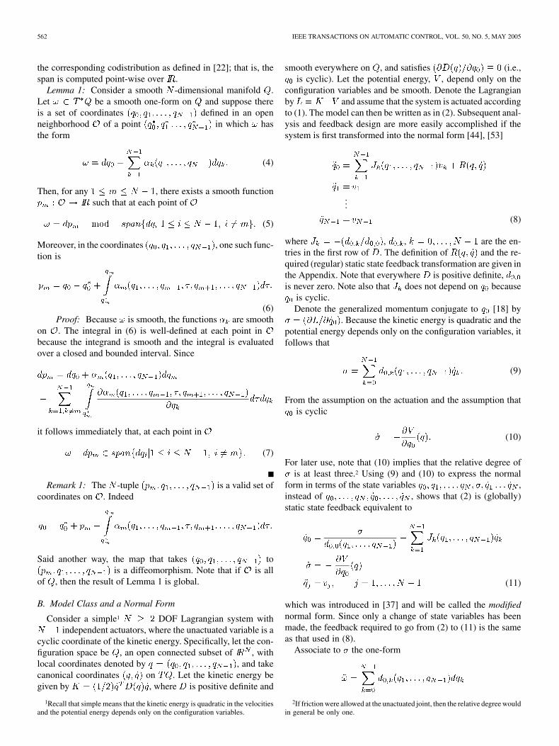
where , , are the en-tries in the first row of . The definition of and the re-quired (regular) static state feedback transformation are given inthe Appendix. Note that everywhere is positive definite,is never zero. Note also that does not depend on because

is cyclic.Denote the generalized momentum conjugate to [18] by

. Because the kinetic energy is quadratic and thepotential energy depends only on the configuration variables, itfollows that

(9)

From the assumption on the actuation and the assumption thatis cyclic

(10)

For later use, note that (10) implies that the relative degree ofis at least three.2 Using (9) and (10) to express the normal

form in terms of the state variables ,instead of , shows that (2) is (globally)static state feedback equivalent to

(11)

which was introduced in [37] and will be called the modifiednormal form. Since only a change of state variables has beenmade, the feedback required to go from (2) to (11) is the sameas that used in (8).

Associate to the one-form

2If friction were allowed at the unactuated joint, then the relative degree wouldin general be only one.


and the normalized one-form

Applying Lemma 1 for , define the function

(12)

Direct computation then leads to

(13)

where

Note that since does not depend on , it must be differen-tiated at least twice more before appears; in other words,has at least relative degree three with respect to .

This concludes the preliminary analysis required for subse-quent feedback design.

C. Systems Where the Generalized Momentum Conjugate tothe Cyclic Variable is not Conserved

It is first assumed that , the generalized momentum conju-gate to , is not constant along solutions of the model (1); thatis

(14)

It is also assumed that there exists a static equilibrium pointcorresponding to some constant value of the control, and

that when defining via (12), is taken as so that van-ishes3 at the equilibrium point. In this case, conditions will beidentified under which the set of outputs

...

(15)

a constant, yields an exponentially minimum phasesystem. More precisely, conditions will be given such that thezero dynamics is well defined in a neighborhood of the givenequilibrium point, has dimension one, and is exponentially

3Alternatively, let q be arbitrary, for example, zero, and define y = K(p �p ) + �, where p is the value at the equilibrium point, q .

stable for all , and moreover, the system is dynamicallyinput–output decouplable (equivalently, invertible).

Before proceeding with the analysis, the intuition behind thischoice of outputs is discussed. As stated earlier, a more standardchoice of outputs would be , for ,where each component has relative degree two. Such a choiceleads to a two-dimensional zero dynamics, which can be shownto be once again a Lagrangian system [56], and thus can neverhave an asymptotically stable equilibrium. By seeking an outputcomponent with a relative degree higher than two, the dimen-sion of the zero dynamics can be reduced, opening up the possi-bility of either having no zero dynamics at all, or, of creating onethat is scalar and asymptotically stable. For the class of systemsbeing studied, no output function of relative degree four hasbeen found (see Section V-B for more discussion on this point).The most obvious relative degree three function available is theconjugate momentum , which is a linear combination of thevelocity components. If the first component of the outputs weremodified to , the resulting zero dynamics manifold wouldinclude a one-dimensional submanifold of equilibria associatedwith and, thus, asymptotic sta-bility of the zero dynamics would be impossible. Inspired by [5],by associating to a one-form and then partially integrating it, afunction was determined that depends only on the configura-tion variables and has at least relative degree three with respectto one of the input components (after a static feedback was usedto put the system in normal form). Hence, any function ofand has at least relative degree three with respect to that inputcomponent. Moreover, by (13), if , for ,then is proportional to through the strictly positive quantity

. Thus the choice , , and ,for , should lead to the exponentially stablezero dynamics .

The main result is now stated.Theorem 1: Consider the simple mechanical system (2) with

DOF, independent actuators and the unactuatedcoordinate is cyclic. Associate to the system the outputs definedin (15), with , and define

(16)Then, in a neighborhood of any equilibrium point at whichis nonzero, the system is

i) exponentially minimum phase;ii) dynamically, input–output decouplable.

Moreover, once the system is transformed into the normal formof (8), or into the modified normal form of (11), then the dy-namic extension

...

(17)


renders it statically input–output decouplable.Proof: The zero dynamics is invariant under regular static

state feedback and dynamic extensions [22]. Hence, assume thesystem has already been transformed into the normal form (11)and then apply the dynamic extension (17). It follows that

, for . It remains to differentiate the first outputcomponent. Equation (13) yields

(18)

The arguments will now be dropped so that theformulas remain compact and readable. Differentiating (18)again yields

(19)

Due to the dynamic extension (17), have at leastrelative degree three and has at least relative degree two, thusthe inputs do not appear in . Differentiating once moreand keeping track only of the terms where the inputs appearyield

(20)

where is given in (16). Therefore, the decoupling matrix is

(21)

and is invertible at a given point if, and only if, is nonzeroat that point. In a neighborhood of an equilibrium point ,

is nonzero if, and only if

(22)

Wherever the decoupling matrix is invertible, the zerodynamics is locally well defined and the set of differentials,

, is independent [22] and,hence, has dimension . System (11) with the dynamicextension (17) has dimension , and thus the zero dy-namics has dimension one. To determine the zero dynamics, itis enough to find a function whose differential is independentof . In the Appendix, it isshown that is an appropriate choice. On the zero dynamicsmanifold (that is, when ), , ,and , . Thus, from (13) [seealso (78) in the Appendix], in a neighborhood of an equilibriumpoint where , the zero dynamics is

(23)

Since is positive, the zero dynamics is exponentially stablefor all .

Remark 2: Note that an integrator has not been added on .This is because is designed to have relative degree three withrespect to , while it only has relative degree two with respectto . With the dynamic extension, has relativedegree three with respect to .

Remark 3: From [22], exponential minimum phase pluslocal static input-output decouplability after a dynamic ex-tension implies the existence of a feedback that induces localasymptotic tracking of output trajectories with internallybounded states. See the three-link robot in Section IV-C-2 foran example.

Remark 4: If in (12) is selected with , then thedynamic extension becomes

(24)

and the decoupling matrix is invertible in a neighborhood of anequilibrium point if, and only if

(25)

Choosing different values of may be useful for avoiding sin-gularities.

Remark 5: The results of the Theorem 1 are inherently localfor two reasons. First of all, the decoupling matrix typically hassingularities away from the equilibrium point (see the examplesin Section IV). Second, even if the decoupling matrix were glob-ally invertible and if the zero dynamics were globally exponen-tially stable, global asymptotic stabilizability of an equilibriumdoes not necessarily follow; see [22, Ch. 9]. A global feedfor-ward representation of the system is discussed in Section V-A;see also [37].

D. Systems Where the Generalized Momentum Conjugate tothe Cyclic Variable is Conserved

It is now assumed that , the generalized momentum conju-gate to , is constant along solutions of the model; that is

(26)

which is equivalent to . In (11), can be treated as aconstant, yielding the reduced-order model

(27)


Let be given and define as in (12). In this case,conditions will be given such that (27) with outputs

...

(28)

is locally, dynamically, feedback linearizable. Note that (28) isa simplification of (15) arising from .

Theorem 2: Consider a simple mechanical system (2) withDOF, independent actuators, and the unactuated

coordinate is cyclic. Suppose that the generalized momentumconjugate to the cyclic coordinate is conserved along the mo-tions of the system so that the reduced system (27) can be de-fined. Associate to (27) the outputs defined in (28) and define

(29)

Then, in a neighborhood of any point at which is nonzero,the following hold.

i) System (27) is dynamically feedback equivalent to acontrollable linear system.

ii) System (27) is the strongly accessible part of (2), andcan be viewed as a representation of the uncon-

trollable part.iii) System (2) is dynamically feedback equivalent to a

linear system with a one-dimensional uncontrollablepart.

iv) System (27) with outputs (28) is dynamically input-output decouplable and has no zero dynamics.

Moreover, the dynamic extension (17) renders (27) staticallyfeedback linearizable.

Proof: As in the proof of Theorem 1, apply to (27) thedynamic extension (17). Once again, , for

and it remains to differentiate the first output component.From (18)–(20), by taking and , itfollows that

(30)

(31)

(32)

Thus, the decoupling matrix is

(33)

and is invertible in a neighborhood of a given point if and onlyif is nonzero at that point. In a neighborhood of a point

where the decoupling matrix is invertible, the sum of the rela-tive degrees of the outputs is , which equals the sumof the dimensions of (27) and (17). It follows that (27) with out-puts (28) has no zero dynamics [22], and thus any regular staticfeedback that locally input-output linearizes (27), (28), and (17),also renders the closed-loop system locally input-to-state linearin the coordinates ; the associ-ated Brunovsky canonical form is , .

Corollary 1: The same results hold for (3) with the exceptionthat the uncontrollable part has dimension five

(34)

where is a constant.

IV. EXAMPLES

This section will illustrate the theoretical results of Section IIIon systems of the type depicted in Figs. 1 and 2. The systems arechosen to be simple enough that the calculations are straight-forward and sufficiently complex to illustrate a range of pos-sible applications of the main theorems. The first example treatsa robot with two rigid links connected via an actuated revo-lute joint and attached at one end to a pivot; that is, the Ac-robot. A novel feature is that the robot is placed on a frictionlesshorizontal plane to remove gravity. If nothing else were done,the angular momentum about the attachment point would beconserved, so stabilization about an equilibrium would not bepossible. A spring is therefore added between the world frameand the first link, and a stabilizing controller is then designedthrough the use of Theorem 1. The second example treats a robotconsisting of three serial links connected by independently ac-tuated revolute joints, attached to a pivot, and constrained toevolve in a vertical plane. For this system, the results of [5], [38]are not applicable for designing a stabilizing controller. The-orem 1 is applied to design a controller that achieves stabiliza-tion about an equilibrium point and asymptotic tracking of tra-jectories. The last problem studied focuses on ballistic motionin a vertical plane, which is a key part of a model of running. Themodel assumes a robot with two rigid links connected via an ac-tuated revolute joint. The angular momentum about the center ofmass is conserved, creating a nonholonomic constraint. Corol-lary 1 is applied to feedback linearize the accessible part of thesystem. The linear representation of the dynamics is shown to beadvantageous for path planning. The singularities that preventthe system from being globally linearized are explicitly notedand how to plan a path through such a singularity is illustrated.

A. Computing the Outputs

The key to applying the results of Section III is the explicitcomputation of the function in (12) used to define the outputs.For all of the examples treated here, plus a wide range of otherexamples, the computation of this function is handled by thefollowing lemma. The proof by direct symbolic integration isnot given.


Lemma 2: Consider a simple mechanical system of the form(2), with DOF and mass inertia matrix . Suppose that

and can be expressed as

(35)

where , and that . Then,for and , (12) can be evaluated explicitlyas

(36)

where

(37)

Remark 6: Write

so that and

Hence, everywhere that , it follows thatand . Therefore, is

a positive real number everywhere that . Theminimum value ofover is equal to ,which is, therefore, also positive everywhere that

. The corresponds to the principal value. If, then (12) can be evaluated explicitly as

.Remark 7: If and either or

, then . In this case, the results simplify to theresults obtained in [38].

Remark 8: For a general point of interest , (12) canbe evaluated as

which is just in (36) minus the same function evaluated at .

B. Planar Two-Link Structure Attached to a Pivot

This example treats the planar two-link robot depicted inFig. 3. The purpose of the example is to emphasize the roleof the potential energy in determining whether generalized

Fig. 3. Two-link robot attached to a pivot and constrained to move in ahorizontal plane. The joint q is actuated, while q is passive; a linear springwith stiffness K is attached with rest position q = 0. From left to right, thelinks have length L and L and the masses are m and m .

momentum is conserved, and to demonstrate in the simplestpossible setting the computations needed to apply Theorem 1in order to achieve asymptotic stabilization of an equilibrium.The robot consists of two point masses connected by two rigid,massless links, with the links joined by an actuated revolutejoint (the use of a distributed mass model would not changeany of the following analysis). The connection to the pivot isunactuated and frictionless.

The configuration variables are chosen as and , whereis the angle of the first link referenced to a world frame attachedto the pivot point and is the relative angle between links oneand two. A linear spring of stiffness is introduced betweenthe first link and the world frame, with rest position .The plane of movement is assumed to be horizontal, and thusthe acceleration due to gravity is . The case where thegravity is non zero can be found in [5].

1) Mathematical Representation: The dynamic model iseasily obtained with the method of Lagrange and verifies thatis a cyclic variable. The complete dynamic model is not given;instead, the system is immediately written in the modifiednormal form (11) as

(38)

where

(39)

In (38), note that , given by (9), is the usual angular mo-mentum of the robot about the attachment point. Since the robot


is constrained to a horizontal plane, if the spring constant werezero, then angular momentum would be conserved and asymp-totic stabilization to an equilibrium point would be impossible.

2) Control Law Design: The control law design consistsof the preliminary feedback needed to place the system in the(modified) normal form (as explained in the Appendix), thedefinition of an output, and a second static state feedback usedto linearize and stabilize the resulting input-output map. Forthe two-link robot, the output is selected as

(40)

where is to be chosen

(41)

and is the value of at the equilibrium of interest, .For single-input systems, the dynamic extension (17) is

trivial: . Since it only amounts to relabeling the input,it is dropped. Direct calculation confirms that has relativedegree three

(42)

where

(43)

Suppose that . Let real scalars , and bechosen such that is exponentiallystable. Then, (43) leads to the locally input-output linearizingand exponentially stabilizing control law[22]

(44)

The actual torque applied to the actuated joint is computed from(75) of the Appendix.

3) Simulation: For the simulations, the robot is assumedconstrained to a horizontal plane , the spring attachingthe first link to the reference frame is assumed linear with

Fig. 4. Stabilization to an equilibrium. The figure shows the convergence ofthe commanded output, its first two derivatives, and the configuration variables.

stiffness , and the model parameters are selected as, , , and . The equilibrium

point was chosen as , , which corresponds to, and satisfies . The scalars were

arbitrarily chosen to place the eigenvalues of the error equationat 1.3. The free parameter in the output was arbitrarily set to

. Since , the zero dynamics has a slightlyslower speed of convergence than the output error equation.

The state feedback controller (44) was simulated for the ini-tial condition , , , . Fig. 4shows the evolution of the commanded output and its deriva-tives along with the evolution of the configuration variables ofthe robot. The output rapidly converges to zero and the config-uration variables converge to the desired equilibrium point. Ananimation of the motion is available at [19].

C. Planar Three-Link Serial Structure Attached to a Pivot

This example treats the planar three-link robot depicted inFig. 5. The robot consists of three point masses connected bythree rigid, massless links, with the links joined by an actuatedrevolute joint. The connection to the pivot is unactuated and fric-tionless. The links are labeled through starting from thepivot and the masses are similarly labeled through . Theparameter values given in Table I were selected to approximatethe biped robot RABBIT with the legs held together [7]. Theconfiguration variables are chosen as through , where isthe angle of the first link referenced to a world frame attachedto the pivot point, is the relative angle between links one andtwo, and is the relative angle between links two and three.No springs are used. The plane of movement is assumed to bevertical and, thus, the acceleration due to gravity is .

The example further illustrates the application of Theorem 1through the use of an output component that has relative degreethree with respect to only one of the input components and theuse of a nontrivial dynamic extension in the design of the feed-back controller. Both local asymptotic tracking and exponentialstabilization to an equilibrium point are demonstrated.


Fig. 5. Three-link mechanism, connected at a pivot, consisting of point massesand massless bars. The links have length L through L starting at the pivot;the masses arem throughm . (a) Equilibrium pose with the center of gravitycentered over the pivot. (b) Initial condition used in the simulation, with theequilibrium position superimposed in the background.

TABLE IMASS AND LENGTH PARAMETERS FOR THREE-LINK MECHANISM

1) Mathematical Representation: The complete dynamicmodel is easily obtained using the method of Lagrange andyields immediately the modified normal form (11) as

(45)

where

(46)

with , as given in Lemma 2, (35). Note that is theangular momentum of the robot about the attachment point andis computed from the previous data via (9).

2) Control Law Design: The goal is to demonstrate localexponential stability and asymptotic tracking about an equi-librium point. An equilibrium point was found from

, , and ,resulting in ; see Fig. 5(a).

The control law design consists of the preliminary feedbackneeded to place the system in the (modified) normal form (asexplained in the Appendix), the selection of two outputs, the dy-namic extension that renders the system statically decouplable(and, hence, statically input-output linearizable), and a secondstatic state feedback used to linearize and stabilize the input-output map. For the three-link robot, the outputs have been se-lected as

(47)

where is to be chosen, and the function is determinedthis time via Remark 8. The dynamic extension is

(48)

which consists of adding a single integrator on . Introduce astate vector , and express the com-position of (45), (47), and (48) as

(49)

Direct calculation confirms that has (vector) relative degreethree [22] with respect to . Indeed, using Lie derivative nota-tion, the output derivatives are

(50)

where corresponds to the decoupling matrix in (21).Evaluating the right-hand side of (22) at the equilibrium pointgives 2.35, and thus the decoupling matrix is invertible in aneighborhood of this point. It follows that a feedback law thatprovides asymptotic tracking is [22]

(51)for any constant matrices that render the error equation ex-ponentially stable: , for .

For the simulation, the matrices were arbitrarily chosento be diagonal and to place all of the eigenvalues of the errorequation at 1. The free parameter in the output was arbitrarilychosen as . Since , the zero dynamics isabout one-third as fast as the output error equation.


Fig. 6. Demonstration of asymptotic tracking and stabilization for thethree-link mechanism. For the first 40 s, the motion consists of an initialtransient, followed by tracking of sinusoidal trajectories that correspond toknee bends. At 40 s, the reference trajectory is abruptly set to zero, therebycommanding the system to an equilibrium point.

3) Simulation Results: The simulation demonstrates asymp-totic tracking and exponential stabilization. The initial conditionwas taken as (1.1,1.42, 1.80,0,0,0), and is depicted in Fig. 5(b).For the first 40 s, the robot is commanded to track sinusoidal ref-erences that cause it to execute a form of calisthenics, namely,deep knee bends; at 40 s, the references are abruptly set to con-stant values corresponding to the equilibrium point in orderto demonstrate convergence to a constant set point. The asymp-totic convergence of the outputs to the commanded referencesis shown in Fig. 6, along with the evolution of the configurationvariables and the applied joint torques. An animation of the mo-tion is available at [19].

D. Planar Two-Link Structure in Ballistic Motion

This examples illustrates how the locally linearizing coordi-nates of Theorem 2 can be used to advantage in planning a flipgait in a planar two link structure undergoing ballistic motion.The boundary constraints chosen in the flip gait are motivated bybipedal running [8]. The singularities in the decoupling matrixwill be explicitly computed and related to configuration changesof the mechanism.

As shown in Fig. 7, the mechanism consists of three pointmasses joined by two massless bars in an actuated, revolutejoint. The four configuration variables are selected as , ,

, and , where relates the orientation of the mechanismto a world frame and is the relative angle between the twolinks. The mechanism’s position with respect to a world frameis represented by the Cartesian coordinates of its center of mass.The point masses are given by , , ; the bar connecting

to has length and that connecting to haslength .

Fig. 7. Two-link robot undergoing ballistic motion in a vertical plane. Onlythe joint q is actuated. From left to right, the links have length L and L andthe masses are m , m , and m .

1) Mathematical Representation: The complete dynamicmodel is easily obtained using the method of Lagrange andyields immediately the modified normal form (11)

(52)

with control and

(53)

The strongly accessible portion of the model has dimensionthree, and involves , , . Due to ballistic motion, there isa five-dimensional uncontrollable subsystem that is completelydecoupled from the actuated portion of the model, and this isgiven by , , , , . How these two parts interact in a pathplanning problem is explained next.

2) Interaction Through Boundary Conditions: The flightphases of a gymnastic robot, such as a tumbler or a bipedalrunner, are typically short-term motions that alternate withsingle support phases.4 The creation of an overall satisfactorymotion is closely tied to achieving correct boundary conditionsat the interfaces of the flight and single support phases. Thestate of the robot at the end of a flight phase determines theinitial conditions for the single support phase, and consequently

4That is, one end of the mechanism is in contact with a rigid surface, and thecontact point is neither slipping nor rebounding; in other words the contact pointis acting as a pivot.


the state of the robot at the end of a flight phase is typicallymore important than the exact trajectory followed during theflight phase.

At the beginning and end of a flight phase, the robot is in con-tact with a surface, assumed here to be identified with the hori-zontal component of the world frame. Assume furthermore thatthe robot is in single support, with the contact point being eitherthe mass or . In single support, there are two holonomicconstraints that tie the position and velocity of the center of massto those of the angular coordinates; in other words, there is a lossof two degrees of freedom. Conservation of angular momentumthrough yields an additional (nonholonomic) constrainton the angular velocities. In particular, the desired final joint ve-locities must be chosen to satisfy this constraint.

The duration of the flight phase is determined from, with the initial conditions coming from the initial positions

and velocities of the angular coordinates at lift-off, and the endcondition of the height of the center mass coming from the de-sired final configuration of the angular coordinates at touch-down. Once the flight time is known, determining whether ornot there exists a solution of the reduced model

(54)

that is compatible with a given set of initial and final conditionsis a difficult problem: Once a trajectory for is chosen,must be numerically integrated, and if does not have thedesired value, then must be altered. Such an iterative pro-cedure is poorly adapted to online computations. Theorem 2 willbe applied to simplify this task. It should be noted that the valueof the momentum is unknown before the start of the flightphase, and thus it is not even possible to determine the reducedmodel (54) before the initial condition of the robot is known atlift-off.

3) Determining a Ballistic Motion Trajectory in LinearizingCoordinates: Local, input-output linearizing coordinates forthe reduced model (54) are constructed from and its firsttwo derivatives. Define by (41). Direct computation leads to

(55)

(56)

To determine the linearizing control, one more derivative isneeded

(57)

(58)

Wherever , a linearizing feedback can be constructedsuch that

(59)

For arbitrary initial and final conditions of the linear model (59),it is trivial to define a feasible trajectory. Indeed, it suffices to de-fine a three-times continuously differentiable function passingfrom given initial values to given final values. One could evenuse a polynomial of order five or greater.

Since the change of coordinates going from (54) to (59) islocal, not every solution of (59) can be mapped back onto asolution of (54). From (55), , the “global” orientation of therobot, can only be changed through modification of the inertiaparameter, , because the angular momentum is constant. Theinertia term can only be changed through variation of theinternal angle . Since is bounded, so is . These kindsof constraints, which must be applied point-wise in time on thetrajectories of (59), are made explicit by computing the inverseof the coordinate change.

4) Constraints Point-Wise in Time Associated With the Lin-earizing Coordinates: The calculation of , , and in termsof , , and yields

(60)

(61)

(62)

The first equation only admits a solution for, and then has two solutions: One for

and another for . These two domainsfor the cosine define two “configuration classes” of the robot,with the extreme points of the domains corresponding to thelinks being completely folded or unfolded. At the extreme pointsof the domains, attains an extremum and consequently, iszero. At an extreme point of , cannot be determined from(62), which takes the form . Since vanishes at anextreme point, (57) is used with to obtain

(63)with the sign of being determined by continuity (with torquecontrol, there cannot be discontinuities in the velocity). Therobot will then pass through the singularity, and change con-figuration classes.

Consequently, when generating a motion, two casescan present themselves, according to whether the motionstays always in the same configuration class or not. If theinitial and final configuration are in the same configura-tion class, then a trajectory can be generated by imposing

. Both open-loopand feedback controls are equally easily computed startingfrom the linear model. If the initial and final configurations arein different configuration classes, a trajectory can be computedthat passes through a singularity at a single time instance,

, where vanishes. An open-loop control


Fig. 8. Motion of the robot passes from left to right without passing through asingularity. The initial configuration (�� left) and final configuration (��right) belong to the same configuration class. The center of gravity follows aparabolic trajectory.

can be determined as before. On the other hand, a feedbackimplementation is not possible based on inverting in (58).However, since the flight phase is typically of short durationand the input is calculated as a function of the initial conditions,an open-loop control is probably sufficient.

5) Simulation Without Passing Through a Singularity: Themodel parameters were selected as , ,

, , and . For this simulation, the massof the robot is supposed initially in contact with the ground, withconfiguration defined by , , and angularvelocities , . The objective is to transfer the robotat the end of a flight phase so that when the mass of the robottouches the ground, its configuration is ,with angular velocity proportional to and . Theinitial and final configurations are depicted in Fig. 8; they belongto the same configuration class. From the initial conditions ofthe robot and the desired final configuration, the flight time iscomputed as . Conservation of angular momentumimplies that .

The initial and final values of and its first two derivativeswere computed from (41), (55), and (56). A fifth-order polyno-mial of was defined that satisfied these boundary conditions.The resulting trajectories of , , are depicted in Fig. 9;the point-wise in time constraints associated with (60)–(62) aremet. The input torque for the system was computed using (57)and (75) of the Appendix. The resulting trajectories in terms of

and are shown in Fig. 10 and the evolution of the robot in thevertical plane is presented in Fig. 8. An animation of the motionis available at [19].

6) Simulation With Passage Through a Singularity: For thissimulation, the mass of the robot is supposed initially in con-tact with the ground, with configuration defined by ,

and angular velocities , . The objec-tive is to transfer the robot at the end of a flight phase so thatwhen the mass of the robot touches the ground, its configu-ration is , with angular velocity propor-tional to , . The initial and final configurations aredepicted in Fig. 11; they do not belong to the same configura-tion class. From the initial conditions of the robot and the desired

Fig. 9. Based on the initial and final conditions of the flight phase, a trajectoryfor p and its derivatives is derived. The plot shows that _p satisfies theconstraint (�=(a � a )) � _p (t) � (�=(a + a )).

Fig. 10. Computed open-loop control transfers the robot from its initial stateto the desired final state ( ).

final configuration, the flight time is computed as .Conservation of angular momentum implies that .

The initial and final values of and its first two derivativeswere computed as before. So that the robot changes configura-tion class, at , the trajectory was forced to pass througha singularity corresponding to , that is, and

. A seventh-order polynomial in was de-fined that satisfied the six boundary conditions, plus ,

. The resulting trajectories of , ,are depicted in Fig. 12. The corresponding trajectories in termsof and are shown in Fig. 13 and the evolution of the robot inthe plane is presented in Fig. 11. An animation of the motion isavailable at [19].

V. ADDITIONAL TECHNICAL POINTS

This section provides additional discussion on a few pointsthat would have broken the flow of the main developments.


Fig. 11. Motion of the robot passes from left to right, with a singular positionoccurring when the two links are aligned. The initial configuration (� � �� left)and final configuration (� � �� right) belong to different configuration classes.

Fig. 12. Based on the initial and final conditions of the flight phase, a trajectoryfor p and its derivatives is derived. The plot shows that _p hits the constraint�=(a +a ) in the middle of the flight phase, which allows the change in theconfiguration class to occur.

A. A Cascade Structure

The feedback designs of Section III-C that have been illus-trated on the two-link and three-link models have singularitieswhere the decoupling matrix looses rank. Results in [20] showthat (within the category of analytic systems and compensators)achieving an invertible decoupling matrix via dynamic compen-sation is a necessary condition for the existence of a compen-sator that achieves asymptotic tracking of an open set of refer-ence trajectories. Hence, while it is not necessary that the partic-ular decoupling matrix constructed in (21) be invertible, at leastsome other decoupling matrix would have to be invertible forasymptotic tracking to be possible on a larger set.

If one is only trying to accomplish stabilization on a large setand not asymptotic tracking, it is then interesting to considerfeedback designs that avoid the requirement of an invertibledecoupling matrix. One way that this may be approachedfor the systems studied in Section III-C is the following.

Fig. 13. Computed open-loop control transfers the robot from its initial stateto the desired final state ( ).

First, use (13) to rewrite (11) in the coordinatesas

(64)

where

(65)

Define , , , ,, , and .

Then, (64) takes the form of a feedforward nonlinear system

(66)

for which various feedback stabilization methods have been de-veloped [30], [48], [49], [55]. Backstepping suggests consid-ering and as virtual controls [28], leading to the simpler(block-)feedforward system

(67)

For a two-link system, and are empty, leading to the twodimensional system , the global asymptotic sta-


bilization5 of which has been studied in [36]. The problem ofasymptotically stabilizing (67) on large sets is open for systemswith three or more links.

B. Checking Feedback Linearizability

This section offers a few observations on the generic non-feedback linearizability of the model class studied here whengeneralized conjugate momentum is not conserved. The reasonto check this property is that if the systems were feedback lin-earizable, then it would be possible to achieve an empty zero dy-namics instead of a zero dynamics with dimension one. Recallthat for single-input systems, it is known that a system is dynam-ically feedback linearizable if, and only if, it is statically feed-back linearizable. For multiple-input systems, dynamic feed-back does enlarge the class of linearizable systems, but nec-essary and sufficient conditions for dynamic feedback lineariz-ability are not known. If one restricts the outputs used to achievedynamic feedback linearizability (often called flat outputs) tobeing only functions of the configuration variables, however,then for mechanical systems with one degree of underactuation,necessary and sufficient conditions for dynamic feedback lin-earization are known [43]; in particular, for the class of systemsbeing studied in this paper, the conclusion is that there do notgenerally exist flat outputs depending only on the configurationvariables.

Consider first a two-DOF system written in the form of (64),and suppose that . Such a system has a single input and,thus, necessary and sufficient conditions for feedback lineariz-ability can be checked. Applying the method of [11], the systemis feedback linearizable if and only if

• either , in which case is a linearizing(or flat) output;

• or, and , where

, in which caseis a linearizing (or flat) output.

These conditions are not generally satisfied for the class of sys-tems being studied; in particular, applying them to the two linkexample of Section IV-B proves that it is not feedback lineariz-able.

Consider next a system with three-DOF written either in theform (11) or (64). Applying once again the method in [11], thesystem is statically feedback linearizable only if

(68)

moreover, the same obstruction persists if an integrator is addedon so the dynamic extension used in this paper does notrender the system static feedback linearizable. The obstruction(68) is present in the three-link example of Section IV-C.

We know of only two mechanical systems that meet theconditions of this paper and are feedback linearizable: Theinertia wheel pendulum [54] and the RTAC or TORA (see [23]and the references therein). Both systems satisfy the condition

5The Lyapunov function used in [36] was not shown to be proper or radiallyunbounded. For the Acrobot, a periodicity property of �G can be used to fill thislacuna when the dynamic model is extended in the obvious way to IR .

, and thus is a linearizing output. The methodof this paper also finds the locally linearizing coordinates. Thisis shown only for the inertia wheel pendulum.

In the coordinates of Fig. 1, the modified normal form of theinertia wheel pendulum is

(69)

where

(70)

and the parameters are as defined in [54]. Since and areconstant, (6) is trivially integrated about the equilibrium point

to obtain

(71)

Defining the output as and using (13) and(18)–(20), the model (69) in the coordinates

becomes

(72)

At the upright equilibrium, and,hence, (72) is linear in the coordinates after theapplication of a static state feedback.

Remark 9: More generally, the underlying reason forthe static feedback linearizability of the inertia wheel pen-dulum can be tied to be the following result, which appliesto DOF mechanisms (2). Consider again the one-form

associated with the gener-alized conjugate momentum (9) and suppose that is closed.Let . Then, a simple computation shows that: a) hasat least relative degree four; b) the outputs ,

, have decoupling matrix (21)with ; c) when the decoupling matrix is invertible,these outputs have vector relative degree (4, 2, , 2) and,thus, the system is static feedback linearizable; and d) thecoordinate transformation required to linearize the system iscanonical and given by , , where

. For the inertia wheelpendulum, is closed because the first row of the inertia matrixis constant; moreover, the relative degree four function isproportional to . In the case of the RTAC, the first row of theinertia matrix is not constant in the appropriate coordinates, but

is still closed.


VI. CONCLUSION

Motivated by a large number of dexterous robots that havebeen introduced in the literature over the past fifteen years, thispaper has analyzed simple planar mechanical systems with anunactuated cyclic variable and an independent actuator for eachshape variable. This class of models is naturally associated withbalancing tasks and includes -link extensions of the Acrobot,the stance phase of Raibert’s hopper and many other robots.Typical control objectives include stabilizing an equilibriumand asymptotically tracking a predefined motion. Through asimple decomposition procedure, models with an unactuatedcyclic variable and an independent actuator for each shape vari-able also arise for certain systems executing a ballistic motion,such as diving, dismounting from a high bar, and tumbling. Forthese systems, since momentum is conserved, since the initialconditions are usually determined by the end of a single supportphase, and since the ballistic phase is usually of short duration,asymptotically tracking a predefined motion is not a reasonableobjective. Instead, the main problem is to determine if a set ofinitial and final conditions is compatible, and if so, to generateonline a trajectory that joins them.

The paper presented two novel control results. When thegeneralized momentum conjugate to the cyclic variable wasnot conserved, conditions were found for the existence of aset of outputs that yielded a one-dimensional, exponentiallystable zero dynamics, along with a dynamic extension thatrendered the system locally input-output decouplable. By ex-isting results, a controller that achieves asymptotic stabilizationand tracking is then easily constructed. When the generalizedmomentum conjugate to the cyclic variable was conserved, areduced system was constructed and conditions were foundfor the existence of a set of outputs that yielded an emptyzero dynamics, along with a dynamic extension that renderedthe system locally input-output decouplable. By existing re-sults, a local coordinate transformation and dynamic feedbackcontroller that linearize the input-to-state map are then easilyconstructed. The solutions to these two control problems had acommon underlying element: The computation of a function ofthe configuration variables that had relative degree three withrespect to one of the input components. It was interesting thatthis function arose by partially integrating a physical quantity,the conjugate momentum.

The theoretical results were illustrated on three simple ex-amples. Stabilization of an equilibrium was demonstrated on avariant of the Acrobot without the influence of gravity. The pur-pose of the example was to emphasize the role of the potentialenergy in determining whether generalized momentum is con-served, and to demonstrate the computations needed to apply theresults of the paper in the simplest possible setting. Asymptoticstabilization about an equilibrium and asymptotic tracking wereboth illustrated on a serial, three-link, mechanism attached to apivot and constrained to evolve in a vertical plane. This exampleprovided a nontrivial illustration of the results for a system withmultiple inputs. The last example illustrated how locally lin-earizing coordinates can simplify the path planning problem fora ballistic flip motion of a two-link mechanism. The singularitiesin the decoupling matrix were explicitly computed and relatedto configuration changes of the mechanism.

APPENDIX

The Normal Form

The normal form is taken from [44] and [53]. Letand partition the generalized

coordinates into actuated and unactuated parts per ,. This induces a decomposition of the

model (2)

(73)

Define

(74)

The static state feedback taking (2) into (8) is

(75)

The feedback is regular because and.

Parameterization of the Zero Dynamics

From the choice of outputs (15), , ;. Hence, to determine the zero dynamics, it is

enough to find a function whose differential is independent of, modulo

(76)

This is most easily done if the model is expressed in the coordi-nates . Then, condition (22) for the invert-ibility of the decoupling matrix at an equilibrium becomes

(77)

where, in the new coordinates, is the equilibrium point andthe potential energy is

Model (8) with the dynamic extension (17) can be rewritten as

(78)


Computing and evaluating their differentials at the equi-librium point and modulo (76), results in

(79)

and, hence,modulo (76). Next, computing and evaluating its dif-ferential at the equilibrium point and modulo (76) and

yields

(80)

and, thus,modulo (76), proving that can be used to parameterize thezero dynamics in a neighborhood of an equilibrium point.

REFERENCES

[1] M. Ahmadi and M. Buehler, “Stable control of a simulated one-leggedrunning robot with hip and leg compliance,” IEEE Trans. Robot. Autom.,vol. 13, no. 1, pp. 96–104, Feb. 1997.

[2] M. D. Berkemeier and R. S. Fearing, “Tracking fast inverted trajectoriesof the underactuated Acrobot,” IEEE Trans. Robot. Autom., vol. 15, no.4, pp. 740–750, Aug. 1999.

[3] A. M. Bloch, N. E. Leonard, and J. E. Marsden, “Controlled lagrangiansand the stabilization of mechanical systems I: The first matching the-orem,” IEEE Trans. Autom. Control, vol. 45, no. 12, pp. 2253–2270,Dec. 2000.

[4] F. Bullo and K. M. Lynch, “Kinematic controllability for decoupled tra-jectory planning in underactuated mechanical systems,” IEEE Trans.Robot. Autom., vol. 17, no. 4, pp. 402–412, Aug. 2001.

[5] L. Cambrini, C. Chevallereau, C. H. Moog, and R. Stojic, “Stable trajec-tory tracking for biped robots,” in Proc. 39th IEEE Conf. Decision andControl, Sydney, Australia, Dec. 2000, pp. 4815–4820.

[6] C. Canudas-de-Wit, L. Roussel, and A. Goswani, “Periodic stabilizationof a 1-DOF hopping robot on nonlinear compliant surface,” in Proc.IFAC Symp. Robot Control, Nantes, France, Sep. 1997, pp. 405–410.

[7] C. Chevallereau, G. Abba, Y. Aoustin, F. Plestan, E. R. Westervelt, C.Canduas-de Wit, and J. W. Grizzle, “RABBIT: A testbed for advancedcontrol theory,” IEEE Control Syst. Mag., vol. 23, no. 5, pp. 57–79, Oct.2003.

[8] C. Chevallereau and Y. Aoustin, “Optimal reference trajectories forwalking and running of a biped robot,” Robotica, vol. 19, no. 5, pp.557–569, Sep. 2001.

[9] C. Chevallereau, A. Formal’sky, and D. Djoudi, “Tracking of a joint pathfor the walking of an underactuated biped,” Robotica, vol. 22, pp. 15–28,2004.

[10] C. Chevallereau and P. Sardain, “Design and actuation optimizationof a 4 axes biped robot for walking and running,” in Proc. IEEE Int.Conf. Robotics and Automation, San Francisco, CA, Apr. 2000, pp.3365–3370.

[11] G. Conte, C. H. Moog, and A. M. Perdon, Nonlinear Control Systems:An Algebraic Setting. New York: Springer-Verlag, Mar. 1999, vol. 242,Lecture Notes in Control and Information Science.

[12] M. Fliess, J. Lévine, P. Martin, and P. Rouchon, “Flatness and defect ofnonlinear systems: Introductory theory and examples,” Int. J. Control,vol. 61, pp. 1327–1361, 1995.

[13] , “A Lie-Bäcklund approach to equivalence and flatness of non-linear systems,” IEEE Trans. Autom. Control, vol. 44, no. 5, pp. 922–937,May 1999.

[14] C. Francois and C. Samson, “A new approach to the control of the planarone-legged hopper,” Int. J. Robot. Res., vol. 17, no. 11, pp. 1150–1166,1998.

[15] T. Fukuda and F. Saito, “Motion control of a brachiation robot,” Robot.Auton. Syst., vol. 18, pp. 83–93, Jul. 1996.

[16] T. Geng and X. Xu, “Flip gait synthesis of a biped based on Poincaremap,” in Proc. 2nd Int. Workshop Robot Motion and Control, BukowyDworek, Poland, Oct. 2001, pp. 239–243.

[17] J. M. Godhavn, A. Balluchi, L. Crawford, and S. Sastry, “Path planningfor nonholonmic systems with drift,” in Proc. Amer. Control Conf., Al-buguerque, NM, Jun. 1997, pp. 532–536.

[18] H. Goldstein, Classical Mechanics, 2nd ed. Reading, MA: Addison-Wesley, 1980.

[19] J. W. Grizzle. (2004, Aug.) Publications on robotics and control. [On-line]http://www.eecs.umich.edu/~grizzle/papers/robotics.html

[20] J. W. Grizzle, M. D. Di Benedetto, and F. Lamnabhi-Lagarrigue, “Nec-essary conditions for asymptotic tracking in nonlinear systems,” IEEETrans. Autom. Control, vol. 39, no. 9, pp. 1782–1794, Sep. 1994.

[21] H. Hermes, “Involutive subdistributions and canonical forms for distri-butions and control systems,” in Theory and Applications of NonlinearControl Systems, C. I. Byrnes and A. Lindquist, Eds. Amsterdam, TheNetherlands: North-Holland, 1986, pp. 123–135.

[22] A. Isidori, Nonlinear Control Systems: An Introduction, 3rd ed. Berlin,Germany: Springer-Verlag, 1995.

[23] Z. P. Jiang and I. Kanellakopoulos, “Global output-feedback trackingfor a benchmark nonlinear system,” IEEE Trans. Autom. Control, vol.45, no. 5, pp. 1023–1027, May 2000.

[24] Z. P. Jiang and H. Nijmeijer, “Tracking control of mobile robots: A casestudy in backstepping,” Automatica, vol. 33, no. 7, pp. 1393–1399, 1997.

[25] , “A recursive technique for tracking control of nonholonomic sys-tems in chained form,” IEEE Trans. Autom. Control, vol. 44, no. 2, pp.265–279, Feb. 1999.

[26] D. E. Koditschek and M. Buehler, “Analysis of a simplified hoppingrobot,” Int. J. Robot. Res., vol. 10, no. 6, pp. 587–605, 1991.

[27] I. Kolmanovsky, N. H. McClamroch, and V. T. Coppola, “New resultson control of multibody systems which conserve angular momentum,”J. Dyna. Control Syst., vol. 1, no. 4, pp. 447–462, 1995.

[28] M. Kristic, I. Kanellakopoulos, and P. Kokotovic, Nonlinear and Adap-tive Control Design. Adaptive and Learning Systems for Signal Pro-cessing, Communications and Control. New York: Wiley, 1995.

[29] H. G. Lee, Y. M. Kim, and H. T. Jeon, “On the linearization via a re-stricted class of dynamic feedback,” IEEE Trans. Autom. Control, vol.45, no. 7, pp. 1385–1391, Jul. 2000.

[30] J. Mareczek, M. Buss, and M. Spong, “Invariance control for a class ofcascade nonlinear systems,” IEEE Trans. Autom. Control, vol. 47, no. 4,pp. 1636–1640, Apr. 2002.

[31] R. Marino, “On the largest feedback linearizable subsystem,” Syst. Con-trol Lett., vol. 7, pp. 345–351, 1986.

[32] M. Miyazaki, M. Sampei, and M. Koga, “Control of a motion of anAcrobot approaching a horizontal bar,” Adv. Robot., vol. 15, no. 4, pp.467–480, 2001.

[33] M. Miyazaki, M. Sampei, M. Koga, and A. Takahashi, “A controlof underactuated hopping gait systems: Acrobot example,” in Proc.IEEE Conf. Decision and Control, Sydney, Australia, Dec. 2000, pp.4797–4803.

[34] J. Nakanishi, T. Fukuda, and D. E. Koditschek, “Preliminary studiesof a second generation brachiation robot controller,” in Proc. IEEEInt. Conf. Robotics and Automation, Albuquerque, NM, Apr. 1997, pp.2050–2056.

[35] , “A brachiating robot controller,” IEEE Trans. Robot. Autom., vol.16, no. 2, pp. 109–123, Apr. 2000.

[36] R. Olfati-Saber, “Control of underactuated mechanical systems withtwo degrees of freedom and symmetry,” in Proc. Amer. Control Conf.,Chicago, IL, Jun. 2000, pp. 4092–4096.

[37] , “Nonlinear control of underactuated mechanical systems with ap-plications to robotics and aerospace vehicles,” Ph.D. dissertation, Cali-fornia Inst. Technol., Pasadena, CA, Feb. 2001.

[38] , “Normal forms for underactuated mechanical systems with sym-metry,” IEEE Trans. Autom. Control, vol. 47, no. 2, pp. 305–308, Feb.2002.

[39] K. Ono, K. Yamamoto, and A. Imadu, “Control of giant swing motionof a two-link horizontal bar gymnast robot,” Adv. Robot., vol. 15, no. 4,pp. 449–465, 2001.

[40] R. Ortega, M. W. Spong, and F. Gomez-Estern, “Stabilization of under-actuated mechanical systems via interconnection and damping assign-ment,” IEEE Trans. Autom. Control, vol. 47, no. 8, pp. 1218–1233, Aug.2002.

[41] F. Plestan, J. W. Grizzle, E. R. Westervelt, and G. Abba, “Stable walkingof a 7-DOF biped robot,” IEEE Trans. Robot. Autom., vol. 19, no. 4, pp.653–668, Aug. 2003.

[42] M. Raibert, Legged Robots That Balance. Cambridge, MA: MIT Press,1986.

[43] M. Rathinam and R. M. Murray, “Configuration flatness of lagrangiansystems underactuated by one control,” SIAM J. Control Optim., vol.376, no. 1, pp. 164–179, 1998.


[44] M. Reyhanoglu, A. van der Schaft, N. H. McClamroch, and I.Kolmanovsky, “Dynamics and control of a class of underactuatedmechanical systems,” IEEE Trans. Autom. Control, vol. 44, no. 9, pp.1663–1671, Sep. 1999.

[45] P. Rouchon, M. Fliess, J. Levine, and P. Martin, “Flatness, motion plan-ning and trailer systems,” in Proc. 32nd IEEE Conf. Decision and Con-trol, Dec. 1993, pp. 2700–2705.

[46] F. Saito, T. Fukuda, and F. Arai, “Swing and locomotion control for atwo-link brachiation robot,” IEEE Control Syst. Mag., vol. 14, no. 1, pp.5–12, Feb. 1994.

[47] M. Sampei, H. Kiyota, and M. Ishikawa, “Control strategies for mechan-ical systems with various constraints—Control of nonholonomic sys-tems,” in Proc. IEEE Conf. Systems, Man, Cybern. C, Appl. Rev., vol. 3,Tokyo, Japan, 1999, pp. 158–165.

[48] R. Sepulchre, M. Arcak, and A. Teel, “Trading the stability of finitezeros for global stabilization of nonlinear cascade systems,” IEEE Trans.Autom. Control, vol. 47, no. 3, pp. 521–525, Mar. 2002.

[49] R. Sepulchre, M. Jankovic, and P. Kokotovic, Constructive NonlinearControl. Communications and Control Engineering. London, U.K.:Springer-Verlag, 1997.

[50] D. Seto and J. Baillieul, “Control problems in super-articulated me-chanical systems,” IEEE Trans. Autom. Control, vol. 39, no. 12, pp.2442–2453, Dec. 1994.

[51] A. Shiriaev and C. Canudas-de-Wit, “Virtual constraints: A constructivetool for orbital stabilization of underactuated nonlinear systems,” unpub-lished, Sep. 2003.

[52] M. W. Spong, “The swing up control problem for the Acrobot,” IEEEControl Syst. Mag., vol. 15, no. 1, pp. 49–55, Feb. 1995.

[53] , “Energy based control of a class of underactuated mechanicalsystems,” in Proc. IFAC World Congr., San Francisco, CA, 1996, pp.431–435.

[54] M. W. Spong, P. Corke, and R. Lozano, “Nonlinear control of the inertiawheel pendulum,” Automatica, vol. 37, pp. 1845–1851, 2001.

[55] A. Teel, “A nonlinear small gain theorem for the analysis of controlsystems with saturation,” IEEE Trans. Autom. Control, vol. 41, no. 9,pp. 1256–1270, Sep. 1996.

[56] E. Westervelt, J. W. Grizzle, and D. E. Koditschek, “Hybrid zero dy-namics of planar biped walkers,” IEEE Trans. Autom. Control, vol. 48,no. 1, pp. 42–56, Jan. 2003.

[57] M. Yamakita, T. Yonemura, Y. Michitsuji, and Z. Luo, “Stabilization ofAcrobot in upright position on a horizontal bar,” in Proc. IEEE Int. Conf.Robotics and Automation, Washington, DC, May 2002, pp. 3093–3098.

J. W. Grizzle (S’78–M’79–SM’90–F’97) receivedthe Ph.D. degree in electrical engineering from TheUniversity of Texas at Austin in 1983.

Since September 1987, he has been with TheUniversity of Michigan, Ann Arbor, where he is aProfessor of Electrical Engineering and ComputerScience. His research interests have often focusedon theoretical aspects of nonlinear systems and con-trol, including geometric methods for continuous-and discrete-time systems, and observer designin discrete-time. He has been a consultant in the

automotive industry since 1986, where he jointly holds fourteen patents dealingwith emissions reduction through improved controller design. His currentinterest in bipedal locomotion grew out of a sabbatical in Strasbourg, France.

Prof. Grizzle’s awards include: with K.L. Dobbins and J.A. Cook (Ford MotorCompany), 1992 Paper of the Year Award from the IEEE Vehicular TechnologySociety; with G. Abba (Univ. of Metz, France) and F. Plestan (Ecole Centrale,Nantes, France), the 2002 Axelby Award from the IEEE Control Systems So-ciety; and with J. Sun (Univ. of Michigan) and J. Cook (Ford), the 2003 IEEEControl Systems Society Technology Award. He has served as an Associate Ed-itor for the TRANSACTIONS ON AUTOMATIC CONTROL AND SYSTEMS and Sys-tems and Control Letters, Publications Chairman for the 1989 Conference onDecision and Control, on the Control Systems Society’s Board of Governors in1997–1999, and is currently an Associate Editor for Automatica and a Memberof several awards committees.

Claude H. Moog received the Ph.D. degree in auto-matic control and the “Docteur d’Etat” degree, bothfrom the University of Nantes, Nantes, Framce, in1980 and 1987, respectively.

Since 1983, he has been with the CNRS, and cur-rently holds the position of “Directeur de Recherche.”His research interests focus on theoretical aspects ofnonlinear systems and control. He coauthored a bookon algebraic methods for nonlinear control systemswith G. Conte and A.M. Perdon. He has served asan Associate Editor for Systems and Control Letters

since January 2004.

Christine Chevallereau graduated from EcoleNationale Supérieure de Mécanique, Nantes, France,in 1985, and received the Ph.D. degree in controland robotics from Ecole Nationale Supérieure deMécanique, Nantes, France in 1988.

Since 1989, she has been with the CNRS in the In-stitut de Recherche en Communications et Cyberne-tique de Nantes. Her research interests include mod-eling and control of robots, especially control of robotmanipulators and legged robots.

Nonlinear Control of Mechanical Systems With an Unactuated Cyclic Variable

Documents

Transcript of Nonlinear Control of Mechanical Systems With an Unactuated Cyclic Variable