Nonlinear Control Lecture 10: Back Steppingele.aut.ac.ir/~abdollahi/Lec_9_N10.pdfOutlineIntegrator...
33
Outline Integrator Back Stepping More General Form Uncertain Systems Trajectory Tracking Nonlinear Control Lecture 10: Back Stepping Farzaneh Abdollahi Department of Electrical Engineering Amirkabir University of Technology Fall 2010 Farzaneh Abdollahi Nonlinear Control Lecture 10 1/27
Transcript of Nonlinear Control Lecture 10: Back Steppingele.aut.ac.ir/~abdollahi/Lec_9_N10.pdfOutlineIntegrator...
Outline Integrator Back Stepping More General Form Uncertain Systems Trajectory Tracking
Nonlinear ControlLecture 10: Back Stepping
Farzaneh Abdollahi
Department of Electrical Engineering
Amirkabir University of Technology
Fall 2010
Farzaneh Abdollahi Nonlinear Control Lecture 10 1/27
Outline Integrator Back Stepping More General Form Uncertain Systems Trajectory Tracking
Integrator Back Stepping
More General FormBack Stepping for Strict-Feedback Systems
Uncertain Systems
Trajectory TrackingStabilizing ΠStabilizing ∆1
Stabilizing ∆2
Farzaneh Abdollahi Nonlinear Control Lecture 10 2/27
Outline Integrator Back Stepping More General Form Uncertain Systems Trajectory Tracking
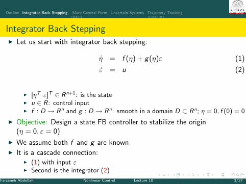
Integrator Back SteppingI Let us start with integrator back stepping:
η = f (η) + g(η)ε (1)
ε = u (2)
I [ηT ε]T ∈ Rn+1: is the stateI u ∈ R: control inputI f : D → Rn and g : D → Rn: smooth in a domain D ⊂ Rn; η = 0, f (0) = 0
I Objective: Design a state FB controller to stabilize the origin(η = 0, ε = 0)
I We assume both f and g are knownI It is a cascade connection:
I (1) with input εI Second is the integrator (2)
Farzaneh Abdollahi Nonlinear Control Lecture 10 3/27
Outline Integrator Back Stepping More General Form Uncertain Systems Trajectory Tracking
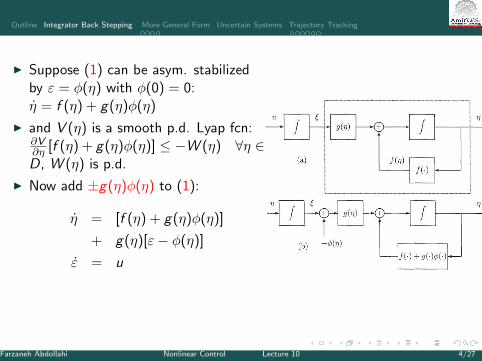
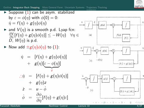
I Suppose (1) can be asym. stabilizedby ε = φ(η) with φ(0) = 0:η = f (η) + g(η)φ(η)
I and V (η) is a smooth p.d. Lyap fcn:∂V∂η [f (η) + g(η)φ(η)] ≤ −W (η) ∀η ∈D, W (η) is p.d.
I Now add ±g(η)φ(η) to (1):
η = [f (η) + g(η)φ(η)]
+ g(η)[ε− φ(η)]
ε = u
Farzaneh Abdollahi Nonlinear Control Lecture 10 4/27
Outline Integrator Back Stepping More General Form Uncertain Systems Trajectory Tracking
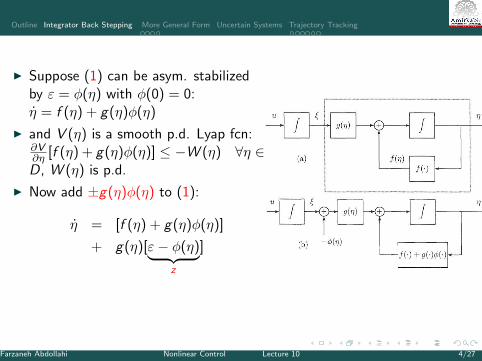
I Suppose (1) can be asym. stabilizedby ε = φ(η) with φ(0) = 0:η = f (η) + g(η)φ(η)
I and V (η) is a smooth p.d. Lyap fcn:∂V∂η [f (η) + g(η)φ(η)] ≤ −W (η) ∀η ∈D, W (η) is p.d.
I Now add ±g(η)φ(η) to (1):
η = [f (η) + g(η)φ(η)]
+ g(η)[ε− φ(η)︸ ︷︷ ︸z
]
Farzaneh Abdollahi Nonlinear Control Lecture 10 4/27
Outline Integrator Back Stepping More General Form Uncertain Systems Trajectory Tracking
I Suppose (1) can be asym. stabilizedby ε = φ(η) with φ(0) = 0:η = f (η) + g(η)φ(η)
I and V (η) is a smooth p.d. Lyap fcn:∂V∂η [f (η) + g(η)φ(η)] ≤ −W (η) ∀η ∈D, W (η) is p.d.
I Now add ±g(η)φ(η) to (1):
η = [f (η) + g(η)φ(η)]
+ g(η)[ε− φ(η)︸ ︷︷ ︸z
]
∴η = [f (η) + g(η)φ(η)]
+ g(η)z
z = u − φ
φ =∂φ
∂η[f (η) + g(η)ε]
Farzaneh Abdollahi Nonlinear Control Lecture 10 4/27
Outline Integrator Back Stepping More General Form Uncertain Systems Trajectory Tracking
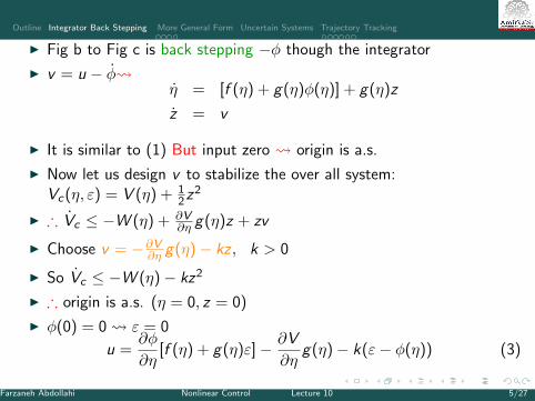
I Fig b to Fig c is back stepping −φ though the integrator
I v = u − φ η = [f (η) + g(η)φ(η)] + g(η)z
z = v
I It is similar to (1) But input zero origin is a.s.
I Now let us design v to stabilize the over all system:Vc(η, ε) = V (η) + 1
2z2
I ∴ Vc ≤ −W (η) + ∂V∂η g(η)z + zv
I Choose v = −∂V∂η g(η)− kz , k > 0
I So Vc ≤ −W (η)− kz2
I ∴ origin is a.s. (η = 0, z = 0)
I φ(0) = 0 ε = 0
u =∂φ
∂η[f (η) + g(η)ε]− ∂V
∂ηg(η)− k(ε− φ(η)) (3)
Farzaneh Abdollahi Nonlinear Control Lecture 10 5/27
Outline Integrator Back Stepping More General Form Uncertain Systems Trajectory Tracking
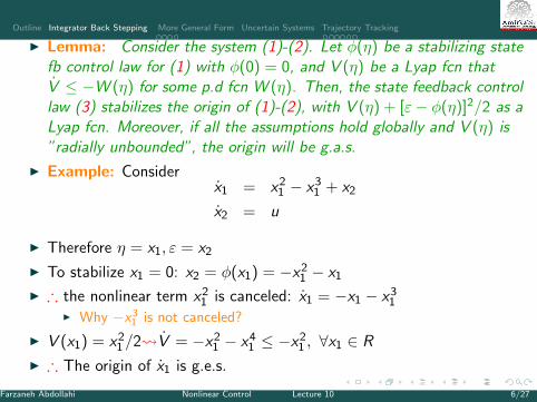
I Lemma: Consider the system (1)-(2). Let φ(η) be a stabilizing statefb control law for (1) with φ(0) = 0, and V (η) be a Lyap fcn thatV ≤ −W (η) for some p.d fcn W (η). Then, the state feedback controllaw (3) stabilizes the origin of (1)-(2), with V (η) + [ε− φ(η)]2/2 as aLyap fcn. Moreover, if all the assumptions hold globally and V (η) is”radially unbounded”, the origin will be g.a.s.
I Example: Considerx1 = x2
1 − x31 + x2
x2 = u
I Therefore η = x1, ε = x2
I To stabilize x1 = 0: x2 = φ(x1) = −x21 − x1
I ∴ the nonlinear term x21 is canceled: x1 = −x1 − x3
1I Why −x3
1 is not canceled?
I V (x1) = x21/2 V = −x2
1 − x41 ≤ −x2
1 , ∀x1 ∈ R
I ∴ The origin of x1 is g.e.s.
Farzaneh Abdollahi Nonlinear Control Lecture 10 6/27
Outline Integrator Back Stepping More General Form Uncertain Systems Trajectory Tracking
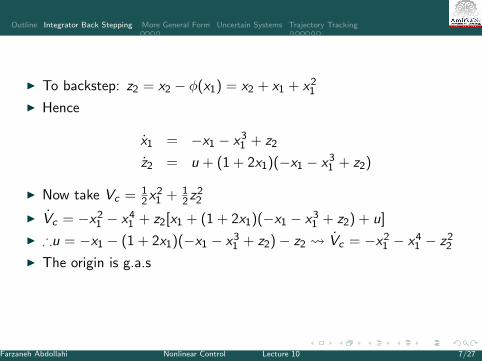
I To backstep: z2 = x2 − φ(x1) = x2 + x1 + x21
I Hence
x1 = −x1 − x31 + z2
z2 = u + (1 + 2x1)(−x1 − x31 + z2)
I Now take Vc = 12x2
1 + 12z2
2
I Vc = −x21 − x4
1 + z2[x1 + (1 + 2x1)(−x1 − x31 + z2) + u]
I ∴u = −x1 − (1 + 2x1)(−x1 − x31 + z2)− z2 Vc = −x2
1 − x41 − z2
2
I The origin is g.a.s
Farzaneh Abdollahi Nonlinear Control Lecture 10 7/27
Outline Integrator Back Stepping More General Form Uncertain Systems Trajectory Tracking
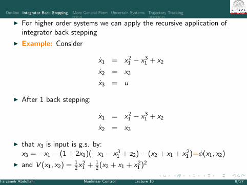
I For higher order systems we can apply the recursive application ofintegrator back stepping
I Example: Consider
x1 = x21 − x3
1 + x2
x2 = x3
x3 = u
I After 1 back stepping:
x1 = x21 − x3
1 + x2
x2 = x3
I that x3 is input is g.s. by:x3 = −x1 − (1 + 2x1)(−x1 − x3
1 + z2)− (x2 + x1 + x21 )=φ(x1, x2)
I and V (x1, x2) = 12x2
1 + 12(x2 + x1 + x2
1 )2
Farzaneh Abdollahi Nonlinear Control Lecture 10 8/27
Outline Integrator Back Stepping More General Form Uncertain Systems Trajectory Tracking
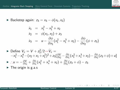
I Backstep again: z3 = x3 − φ(x1, x2)
x1 = x21 − x3
1 + x2
x2 = φ(x1, x2) + z3
x3 = u − ∂φ
∂x1(x2
1 − x31 + x2)− ∂φ
∂x2(φ+ z3)
I Define Vc = V + z23/2 Vc =
−x21 −x4
1 −(x2 +x1 +x21 )2 +z3[ ∂V
∂x2− ∂φ∂x1
(x21 +x3
x +x2)− ∂φ∂x2
(z3 +φ)+u]
I ∴u = − ∂V∂x2
+ ∂φ∂x1
(x21 + x3
x + x2) + ∂φ∂x2
(z3 + φ)− z3
I The origin is g.a.s
Farzaneh Abdollahi Nonlinear Control Lecture 10 9/27
Outline Integrator Back Stepping More General Form Uncertain Systems Trajectory Tracking
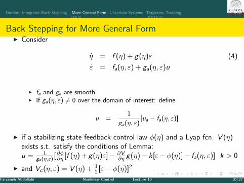
Back Stepping for More General FormI Consider
η = f (η) + g(η)ε (4)
ε = fa(η, ε) + ga(η, ε)u
I fa and ga are smoothI If ga(η, ε) 6= 0 over the domain of interest: define
u =1
ga(η, ε)[ua − fa(η, ε)]
I if a stabilizing state feedback control law φ(η) and a Lyap fcn. V (η)exists s.t. satisfy the conditions of Lemma:u = 1
ga(η,ε)[∂φ∂η [f (η) + g(η)ε]− ∂V
∂η g(η)− k[ε− φ(η)]− fa(η, ε)] k > 0
I and Vc(η, ε) = V (η) + 12 [ε− φ(η)]2
Farzaneh Abdollahi Nonlinear Control Lecture 10 10/27
Outline Integrator Back Stepping More General Form Uncertain Systems Trajectory Tracking
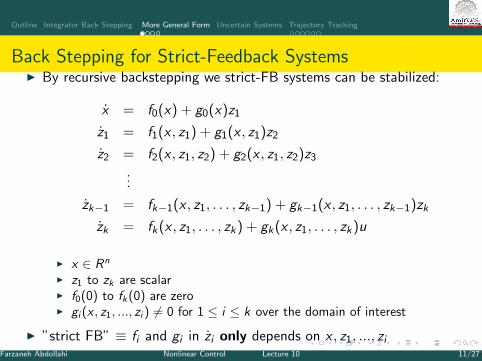
Back Stepping for Strict-Feedback SystemsI By recursive backstepping we strict-FB systems can be stabilized:
x = f0(x) + g0(x)z1
z1 = f1(x , z1) + g1(x , z1)z2
z2 = f2(x , z1, z2) + g2(x , z1, z2)z3
...
zk−1 = fk−1(x , z1, . . . , zk−1) + gk−1(x , z1, . . . , zk−1)zk
zk = fk(x , z1, . . . , zk) + gk(x , z1, . . . , zk)u
I x ∈ Rn
I z1 to zk are scalarI f0(0) to fk(0) are zeroI gi (x , z1, ..., zi ) 6= 0 for 1 ≤ i ≤ k over the domain of interest
I ”strict FB” ≡ fi and gi in zi only depends on x , z1, ..., zi
Farzaneh Abdollahi Nonlinear Control Lecture 10 11/27
Outline Integrator Back Stepping More General Form Uncertain Systems Trajectory Tracking
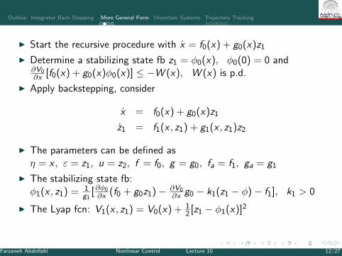
I Start the recursive procedure with x = f0(x) + g0(x)z1
I Determine a stabilizing state fb z1 = φ0(x), φ0(0) = 0 and∂V0∂x [f0(x) + g0(x)φ0(x)] ≤ −W (x), W (x) is p.d.
I Apply backstepping, consider
x = f0(x) + g0(x)z1
z1 = f1(x , z1) + g1(x , z1)z2
I The parameters can be defined asη = x , ε = z1, u = z2, f = f0, g = g0, fa = f1, ga = g1
I The stabilizing state fb:φ1(x , z1) = 1
g1[∂φ0∂x (f0 + g0z1)− ∂V0
∂x g0 − k1(z1 − φ)− f1], k1 > 0
I The Lyap fcn: V1(x , z1) = V0(x) + 12 [z1 − φ1(x)]2
Farzaneh Abdollahi Nonlinear Control Lecture 10 12/27
Outline Integrator Back Stepping More General Form Uncertain Systems Trajectory Tracking
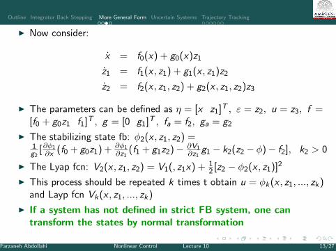
I Now consider:
x = f0(x) + g0(x)z1
z1 = f1(x , z1) + g1(x , z1)z2
z2 = f2(x , z1, z2) + g2(x , z1, z2)z3
I The parameters can be defined as η = [x z1]T , ε = z2, u = z3, f =[f0 + g0z1 f1]T , g = [0 g1]T , fa = f2, ga = g2
I The stabilizing state fb: φ2(x , z1, z2) =1g2
[∂φ1∂x (f0 + g0z1) + ∂φ1
∂z1(f1 + g1z2)− ∂V1
∂z1g1 − k2(z2 − φ)− f2], k2 > 0
I The Lyap fcn: V2(x , z1, z2) = V1(, z1x) + 12 [z2 − φ2(x , z1)]2
I This process should be repeated k times t obtain u = φk(x , z1, ..., zk)and Layp fcn Vk(x , z1, ..., zk)
I If a system has not defined in strict FB system, one cantransform the states by normal transformation
Farzaneh Abdollahi Nonlinear Control Lecture 10 13/27
Outline Integrator Back Stepping More General Form Uncertain Systems Trajectory Tracking
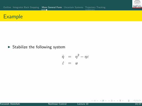
Example
I Stabilize the following system
η = η2 − ηεε = u
Farzaneh Abdollahi Nonlinear Control Lecture 10 14/27
Outline Integrator Back Stepping More General Form Uncertain Systems Trajectory Tracking
Example
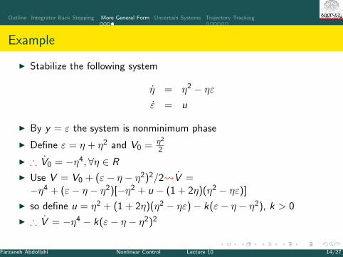
I Stabilize the following system
η = η2 − ηεε = u
I By y = ε the system is nonminimum phase
I Define ε = η + η2 and V0 = η2
2
I ∴ V0 = −η4,∀η ∈ R
I Use V = V0 + (ε− η − η2)2/2 V =−η4 + (ε− η − η2)[−η2 + u − (1 + 2η)(η2 − ηε)]
I so define u = η2 + (1 + 2η)(η2 − ηε)− k(ε− η − η2), k > 0
I ∴ V = −η4 − k(ε− η − η2)2
Farzaneh Abdollahi Nonlinear Control Lecture 10 14/27
Outline Integrator Back Stepping More General Form Uncertain Systems Trajectory Tracking
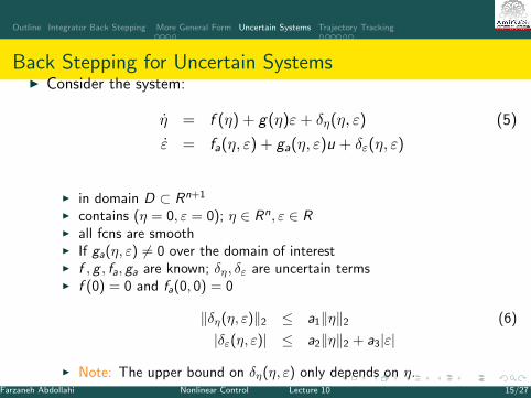
Back Stepping for Uncertain SystemsI Consider the system:
η = f (η) + g(η)ε+ δη(η, ε) (5)
ε = fa(η, ε) + ga(η, ε)u + δε(η, ε)
I in domain D ⊂ Rn+1
I contains (η = 0, ε = 0); η ∈ Rn, ε ∈ RI all fcns are smoothI If ga(η, ε) 6= 0 over the domain of interestI f , g , fa, ga are known; δη, δε are uncertain termsI f (0) = 0 and fa(0, 0) = 0
‖δη(η, ε)‖2 ≤ a1‖η‖2 (6)
|δε(η, ε)| ≤ a2‖η‖2 + a3|ε|
I Note: The upper bound on δη(η, ε) only depends on η.Farzaneh Abdollahi Nonlinear Control Lecture 10 15/27

Outline Integrator Back Stepping More General Form Uncertain Systems Trajectory Tracking
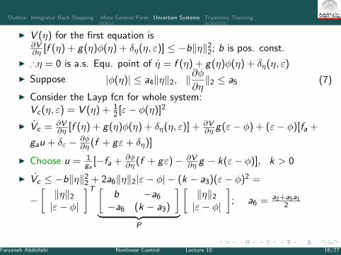
I V (η) for the first equation is∂V∂η [f (η) + g(η)φ(η) + δη(η, ε)] ≤ −b‖η‖22; b is pos. const.
I ∴η = 0 is a.s. Equ. point of η = f (η) + g(η)φ(η) + δη(η, ε)
I Suppose |φ(η)| ≤ a4‖η‖2, ‖∂φ
∂η‖2 ≤ a5 (7)
I Consider the Layp fcn for whole system:Vc(η, ε) = V (η) + 1
2 [ε− φ(η)]2
I Vc = ∂V∂η [f (η) + g(η)φ(η) + δη(η, ε)] + ∂V
∂η g(ε− φ) + (ε− φ)[fa +
gau + δε − ∂φ∂η (f + gε+ δη)]
Farzaneh Abdollahi Nonlinear Control Lecture 10 16/27
Outline Integrator Back Stepping More General Form Uncertain Systems Trajectory Tracking
I V (η) for the first equation is∂V∂η [f (η) + g(η)φ(η) + δη(η, ε)] ≤ −b‖η‖22; b is pos. const.
I ∴η = 0 is a.s. Equ. point of η = f (η) + g(η)φ(η) + δη(η, ε)
I Suppose |φ(η)| ≤ a4‖η‖2, ‖∂φ
∂η‖2 ≤ a5 (7)
I Consider the Layp fcn for whole system:Vc(η, ε) = V (η) + 1
2 [ε− φ(η)]2
I Vc = ∂V∂η [f (η) + g(η)φ(η) + δη(η, ε)] + ∂V
∂η g(ε− φ) + (ε− φ)[fa +
gau + δε − ∂φ∂η (f + gε+ δη)]
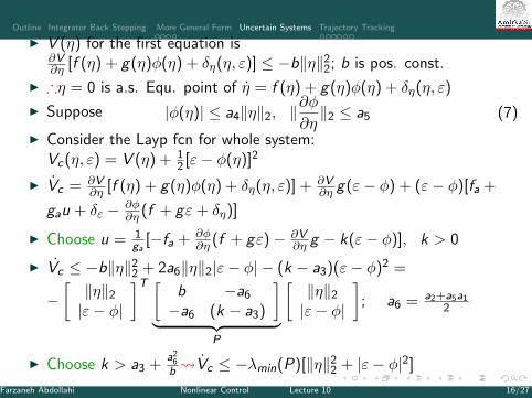
I Choose u = 1ga
[−fa + ∂φ∂η (f + gε)− ∂V
∂η g − k(ε− φ)], k > 0
I Vc ≤ −b‖η‖22 + 2a6‖η‖2|ε− φ| − (k − a3)(ε− φ)2 =
−[‖η‖2|ε− φ|
]T [b −a6
−a6 (k − a3)
]︸ ︷︷ ︸
P
[‖η‖2|ε− φ|
]; a6 = a2+a5a1
2
Farzaneh Abdollahi Nonlinear Control Lecture 10 16/27
Outline Integrator Back Stepping More General Form Uncertain Systems Trajectory Tracking
I V (η) for the first equation is∂V∂η [f (η) + g(η)φ(η) + δη(η, ε)] ≤ −b‖η‖22; b is pos. const.
I ∴η = 0 is a.s. Equ. point of η = f (η) + g(η)φ(η) + δη(η, ε)
I Suppose |φ(η)| ≤ a4‖η‖2, ‖∂φ
∂η‖2 ≤ a5 (7)
I Consider the Layp fcn for whole system:Vc(η, ε) = V (η) + 1
2 [ε− φ(η)]2
I Vc = ∂V∂η [f (η) + g(η)φ(η) + δη(η, ε)] + ∂V
∂η g(ε− φ) + (ε− φ)[fa +
gau + δε − ∂φ∂η (f + gε+ δη)]
I Choose u = 1ga
[−fa + ∂φ∂η (f + gε)− ∂V
∂η g − k(ε− φ)], k > 0
I Vc ≤ −b‖η‖22 + 2a6‖η‖2|ε− φ| − (k − a3)(ε− φ)2 =
−[‖η‖2|ε− φ|
]T [b −a6
−a6 (k − a3)
]︸ ︷︷ ︸
P
[‖η‖2|ε− φ|
]; a6 = a2+a5a1
2
I Choose k > a3 +a26b Vc ≤ −λmin(P)[‖η‖22 + |ε− φ|2]
Farzaneh Abdollahi Nonlinear Control Lecture 10 16/27
Outline Integrator Back Stepping More General Form Uncertain Systems Trajectory Tracking
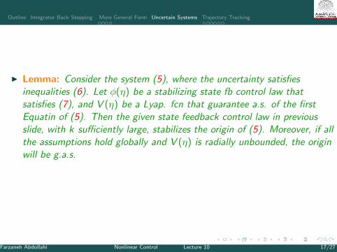
I Lemma: Consider the system (5), where the uncertainty satisfiesinequalities (6). Let φ(η) be a stabilizing state fb control law thatsatisfies (7), and V (η) be a Lyap. fcn that guarantee a.s. of the firstEquatin of (5). Then the given state feedback control law in previousslide, with k sufficiently large, stabilizes the origin of (5). Moreover, if allthe assumptions hold globally and V (η) is radially unbounded, the originwill be g.a.s.
Farzaneh Abdollahi Nonlinear Control Lecture 10 17/27

Outline Integrator Back Stepping More General Form Uncertain Systems Trajectory Tracking
Trajectory Tracking for A Second Order System [1], [2]I A 3 link underactuated manipulator
I The first two translational joints are actuatedI The third revolute joint is not actuatedI The linear approximation of this system is not
controllable since it is not influenced by gravity
I The dynamics:mx rx −m3lsin(θ)θ −m3lcos(θ)θ2 = τ1
my ry + m3lcos(θ)θ −m3lsin(θ)θ2 = τ2
I θ −m3lsin(θ)rx + m3lcos(θ)r)y = 0
λθ + rxsin(θ) + ry cos(θ) = 0
where [rx , ry ]: displacement of third joint; θorientation of third link respect to x axis; τ1 τ2:input of actuated joints; mi : mass, Ii : inertia;λ = (I3 + m3l2)/(m3l)
Farzaneh Abdollahi Nonlinear Control Lecture 10 18/27
Outline Integrator Back Stepping More General Form Uncertain Systems Trajectory Tracking
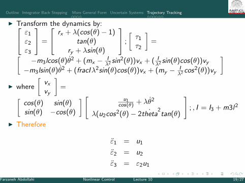
I Transform the dynamics by: ε1ε2ε3
=
rx + λ(cos(θ)− 1)tan(θ)
ry + λsin(θ)
;
[τ1τ2
]=[
−m3lcos(θ)θ2 + (mx − Iλ2 sin2(θ))vx + ( I
λ2 sin(θ)cos(θ))vy
−m3lsin(θ)θ2 + (fracIλ2sin(θ)cos(θ))vx + (my − Iλ2 cos2(θ))vy
]I where
[vx
vy
]=[
cos(θ) sin(θ)sin(θ) −cos(θ)
] [ u1cos(θ) + λθ2
λ(u2cos2(θ)− 2 ˙theta2tan(θ)
]; , I = I3 + m3l2
I Therefore
ε1 = u1
ε2 = u2
ε3 = ε2u1
Farzaneh Abdollahi Nonlinear Control Lecture 10 19/27
Outline Integrator Back Stepping More General Form Uncertain Systems Trajectory Tracking
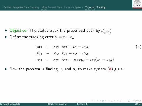
I Objective: The states track the prescribed path by εdij , εdij
I Define the tracking error x = ε− εd
x11 = x12 x12 = u1 − u1d (8)
x21 = x22 x21 = u2 − u2d
x31 = x32 x32 = x21u1d + ε21(u1 − u1d)
I Now the problem is finding u1 and u2 to make system (8) g.a.s.
Farzaneh Abdollahi Nonlinear Control Lecture 10 20/27
Outline Integrator Back Stepping More General Form Uncertain Systems Trajectory Tracking
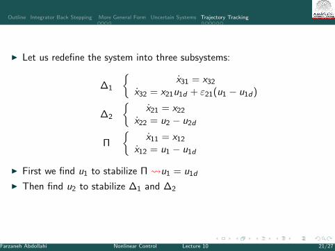
I Let us redefine the system into three subsystems:
∆1
{x31 = x32
x32 = x21u1d + ε21(u1 − u1d)
∆2
{x21 = x22
x22 = u2 − u2d
Π
{x11 = x12
x12 = u1 − u1d
I First we find u1 to stabilize Π u1 = u1d
I Then find u2 to stabilize ∆1 and ∆2
Farzaneh Abdollahi Nonlinear Control Lecture 10 21/27
Outline Integrator Back Stepping More General Form Uncertain Systems Trajectory Tracking
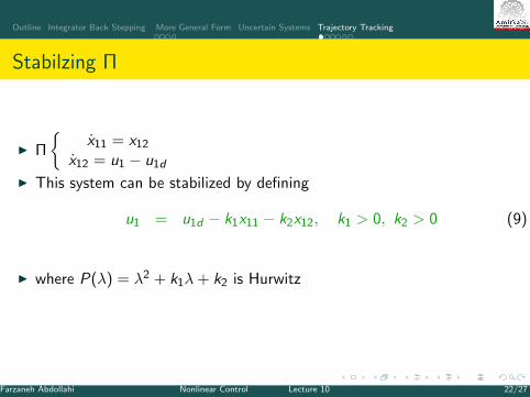
Stabilzing Π
I Π
{x11 = x12
x12 = u1 − u1d
I This system can be stabilized by defining
u1 = u1d − k1x11 − k2x12, k1 > 0, k2 > 0 (9)
I where P(λ) = λ2 + k1λ+ k2 is Hurwitz
Farzaneh Abdollahi Nonlinear Control Lecture 10 22/27
Outline Integrator Back Stepping More General Form Uncertain Systems Trajectory Tracking
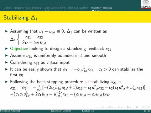
Stabilizing ∆1
I Assuming that u1 − u1d ≡ 0, ∆1 can be written as
∆1
{x31 = x32
x32 = x21u1d
I Objective looking to design a stabilizing feedback x21
I Assume u1d is uniformly bounded in t and smooth
I Considering x32 as virtual input
I It can be easily shown that φ1 = −c1u21dx31, c1 > 0 can stabilize the
first eq.
I Following the back stepping procedure stabilizing x21 isx21 = φ2 = − 1
ud1[−(2c1u1du1d + 1)x13− c1u2
1dx32− c2(c1u41d + u2
1dx32)] =
−(c1c2u31d + 2c1u1d + u−1
1d )x13 − (c1u1d + c2u1d)x32
Farzaneh Abdollahi Nonlinear Control Lecture 10 23/27

Outline Integrator Back Stepping More General Form Uncertain Systems Trajectory Tracking
Stabilizing ∆2
I ∆2
{x21 = x22
x22 = u2 − u2d
I With u1 = u1d , ∆1 is e.sabilized by x12 = φ2
I Apply backstepping to find u2:
I Define x21 = x21 − φ2
I ∴ ˙x21 = x21 − ddt [φ2]
I Now define x22 = x22 − φ3, φ3 = −c3x21 + ddt [φ2]
I It can be easily find that the following u2 can stabilize the system
u2 − u2d = −c4x22 +d
dt[φ3] (10)
= −c3c4x21 − (c3 + c4)x22 + c3c4φ2 + (c3 + c4)d
dt[φ2] +
d2
dt2[φ2]
I It has been shown that (9) and (10) can e.stabilized (8). [1]Farzaneh Abdollahi Nonlinear Control Lecture 10 24/27

Outline Integrator Back Stepping More General Form Uncertain Systems Trajectory Tracking
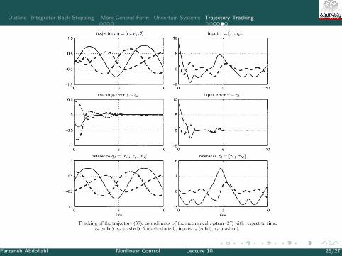
Simulation Results
I For the 3 link manipulator consider the following desired traj:rxd = r1sin(at)− λ(cos(arctan(r2cos(at)))− 1)ryd = r1r2
8 sin(2at)− λsin(arctan(r2cos(at)))θd(t) = arctan(r2cos(at))
I Define: r1 = r2 = a = 1, k1 = 4, k2 = 2√
2, c1 = 2, c2 = 2, c3 = 4, c4 = 4
I The results of tracking is shown in Figs.
Farzaneh Abdollahi Nonlinear Control Lecture 10 25/27
Outline Integrator Back Stepping More General Form Uncertain Systems Trajectory Tracking
Farzaneh Abdollahi Nonlinear Control Lecture 10 26/27

Outline Integrator Back Stepping More General Form Uncertain Systems Trajectory Tracking
Farzaneh Abdollahi Nonlinear Control Lecture 10 27/27
Outline Integrator Back Stepping More General Form Uncertain Systems Trajectory Tracking
N. P. Aneke,y. H. Nijmeijerz, and A. G. Jager, “Trackingcontrol of second-order chained form systems by cascadedbackstepping,” International Journal of Robust and NonlinearControl vol. 95, no.115 , pp. 95–115, 2003.
A. Isidori, F.L. Lagarrigue, W. Respondek, Nonlinear Controlin The Year 2000.Springer, 2001.
Farzaneh Abdollahi Nonlinear Control Lecture 10 27/27