J . Fluid Mech. (1975), wol. 68, part 1, pp . 21-40

Printed in Great Britain 21

Nonlinear calculation of arbitrarily shaped supercavitating hydrofoils near a free surface

By OKITSUGU FURUYA Division of Engineering and Applied Science, California Institute of

Technology, Pasadenat

(Received 15 December 1973)

A nonlinear exact solution to the problem of two-dimensional gravity-free incompressible potential flow around an arbitrarily shaped supercavitating hydrofoil near a free surface is obtained. A combination of Newton’s method with a functional iterative procedure is used to solve the nonlinear integral and algebraic equations of this problem. Fast and stable convergence results by starting the iteration with a readily chosen initial solution. Some representative numerical computations are made for practical hydrofoils having both generally shaped camber and leading-edge thickness distributions. The force coefficients, pressure distribution and free-streamline shapes of the cavity are calculated for each case with an execution time on an IBM 370-158 of 200-530s depending upon the initial trial solution.

1. Introduction In order to design a practical supercavitating hydrofoil operating near a free

surface, a close investigation of flow details such as the pressure distribution and cavity shape as well as the overall force and moment coefficients is required. Yet no appropriate method for this purpose having full accuracy yet permitting efficient computation has been derived (see, for example, the latest review articles on cavity flows by Wu (1972) and on hydrofoils by Acosta (1973)). The linearized free-streamline theory of Tulin (1953), for example, is a simple, direct but approximate method for predicting the forces on thin bodies and has been widely applied generally and applied to the present problem for a flat-plate foil by Yim (1 964). Unfortunately, this theory fails to calculate the pressure distribution correctly because of the singularities required at the leading edge by the theory itself. These singularities may be removed (Furuya & Acosta 1973) by employing a local nonlinear solution near the leading edge, still within the restrictions of overall small camber and SO on. The nonlinear exact theory is no doubt superior, provided that the nonlinear calculations themselves can be carried out, in that all the above features can be provided to high accuracy without any limitations on the flow configuration. The basic theory itself goes back to Levi-Civita (1907; see, for example, Gilbarg 1960; Milne-Thomson 1968). However, the nonlinearity ofthe theory has long been the barrier to its general use. This occurs because the

t Present address: Tetra Tech. Inc., Pasadena, California 91107.

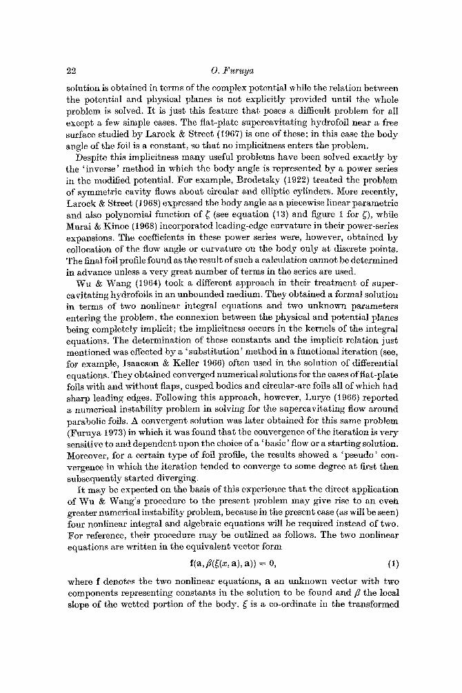
22 0. Furuya

solution is obtained in terms of the complex potential while the relation between the potential and physical planes is not explicitly provided until the whole problem is solved. It is just this feature that poses a difficult problem for all except a few simple cases. The flat-plate supercavitating hydrofoil near a free surface studied by Larock & Street (1967) is one of these; in this case the body angle of the foil is a constant, so that no implicitness enters the problem.

Despite this implicitness many useful problems have been solved exactly by the ‘inverse’ method in which the body angle is represented by a power series in the modified potential. For example, Brodetsky (1922) treated the problem of symmetric cavity flows about circular and elliptic cylinders. More recently, Larock & Street (1968) expressed the body angle as a piecewise linear parametric and also polynomial function of y (see equation (13) and figure 1 for C), while Murai & Kinoe (1968) incorporated leading-edge curvature in their power-series expansions. The coefficients in these power series were, however, obtained by collocation of the flow angle or curvature on the body only at discrete points. The final foil profile found as the result of such a calculation cannot be determined in advance unless a very great number of terms in the series are used.

Wu & Wang (1964) took a different approach in their treatment of super- cavitating hydrofoils in an unbounded medium. They obtained a formal solution in terms of two nonlinear integral equations and two unknown parameters entering the problem, the connexion between the physical and potential planes being completely implicit; the implicitness occurs in the kernels of the integral equations. The determination of these constants and the implicit relation just mentioned was effected by a ‘substitution’ method in a functional iteration (see, for example, Isaacson & Keller 1966) often used in the solution of differential equations. They obtained converged numerical solutions for the cases of flat-plate foils with and without flaps, cusped bodies and circular-arc foils all of which had sharp leading edges. Following this approach, however, Lurye (1 966) reported a numerical instability problem in solving for the supercavitating flow around parabolic foils. A convergent solution was later obtained for this same problem (Furuya 1973) in which it was found that the convergence of the iteration is very sensitive to and dependent upon the choice of a ‘basic ’ flow or a starting solution. Moreover, for a certain type of foil profile, the results showed a ‘pseudo’ con- vergence in which the iteration tended to converge to some degree at first then subsequently started diverging.

It may be expected on the basis of this experience that the direct application of Wu & Wang’s procedure to the present problem may give rise to an even greater numerical instability problem, because in the present case (as will be seen) four nonlinear integral and algebraic equations will be required instead of two. For reference, their procedure may be outlined as follows. The two nonlinear equations are written in the equivalent vector form

where f denotes the two nonlinear equations, a an unknown vector with two components representing constants in the solution to be found and p the local slope of the wetted portion of the body. is a co-ordinate in the transformed

Arbitrarily shaped supercavitating hydrofoils 23

potential plane and x is that in the physical plane. It should be mentioned that the system (1) is entirely different from the usual set of nonlinear equations in that it involves an implicit function P ( f x ) ) as well as the unknown parameters a, where 51%) will be found if a and P(5) are given. We can always write (1) as

( 2 )

(3) where the subscript v denotes the number of the iteration. By starting the iteration with a basic flow whose solution (al, Pl) is known, a2 and P2(,E) can be calculated from (3). This process of substitution is repeated until

a = g(a,P(5(x, a), a))

a,+, = g(a,,Py(5(x, a"), a,))?

and the iterative loop can be established by writing ( 2 ) as

11 (%+I - %)/%+ill 7 7 etc.9

becomes smaller than a desired value. This is in essence the substitution method used by Wu & Wang (1964).

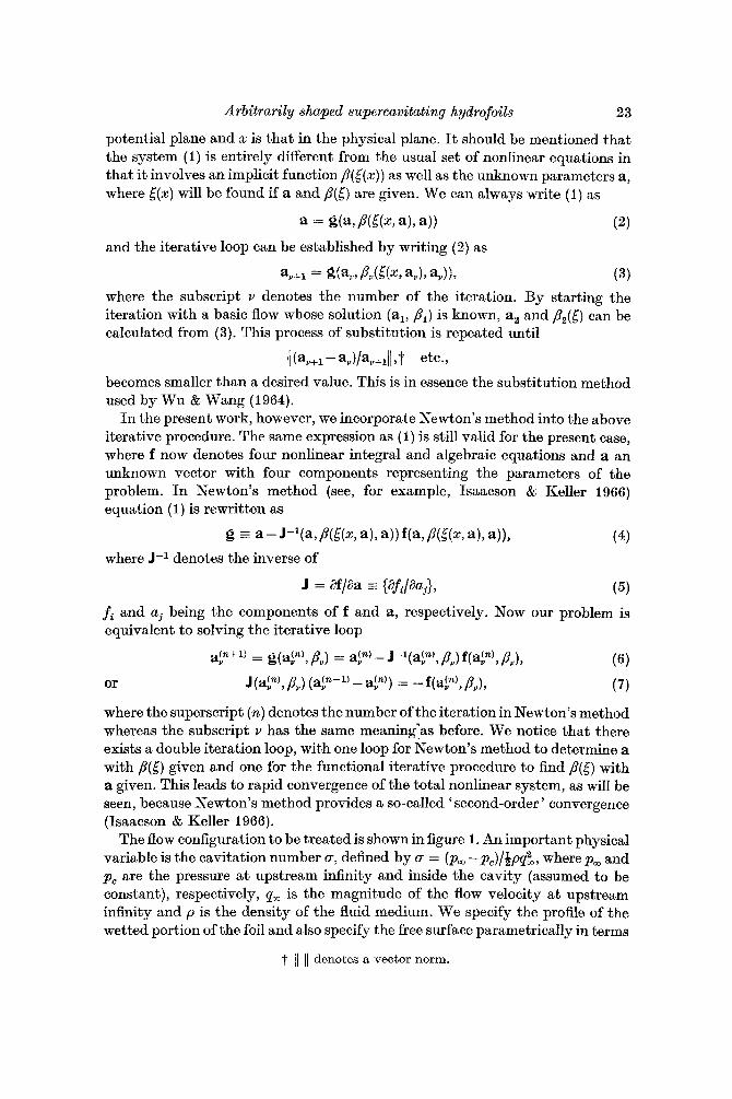
In the present work, however, we incorporate Newton's method int,o the above iterative procedure. The same expression as (1) is still valid for the present case, where f now denotes four nonlinear integral and algebraic equations and a an unknown vector with four components representing the parameters of the problem. In Newton's method (see, for example, Isaacson & Keller 1966) equation (1) is rewritten as

$2 = a - J - l ( a , P ( k a), a)) f(a, P ( t ( X > a), a)), (4) where J-l denotes the inverse of

J = af/aa z {afi/aaj>,

fi and aj being the components of f and a, respectively. Now our problem is equivalent to solving the iterative loop

(6)

or J(al"),Pv) (a:?Z+l)-a:")) = -f(ainn',PY), (7)

a:"+l) = g(a$"), P,) = a?) - J-l(a(") Y 7 P") f(aS"'t P A

where the superscript (n) denotes the number of the iteration in Newton's method whereas the subscript v has the same meaning:as before. We notice that there exists a double iteration loop, with one loop for Newton's method to determine a with P(5) given and one for the functional iterative procedure t o find P ( t ) with a given. This leads to rapid convergence of the total nonlinear system, as will be seen, because Newton's method provides a so-called ' second-order ' convergence (Isaacson & Keller 1966).

The flow configuration to be treated is shown in figure 1. An important physical variable is the cavitation number cr, defined by = (pm -pc)/&pq:, wherep, and pc are the pressure a t upstream infinity and inside the cavity (assumed to be constant), respectively, qm is the magnitude of the flow velocity a t upstream infinity and p is the density of the fluid medium. We specify the profile of the wetted portion of the foil and also specify the free surface parametrically in terms

t /I 11 denotes a vector norm.

24

I;"/

0. Furuya

/ u r e c surface, p=pm -D'

I

,-T =+ In (1+u) I

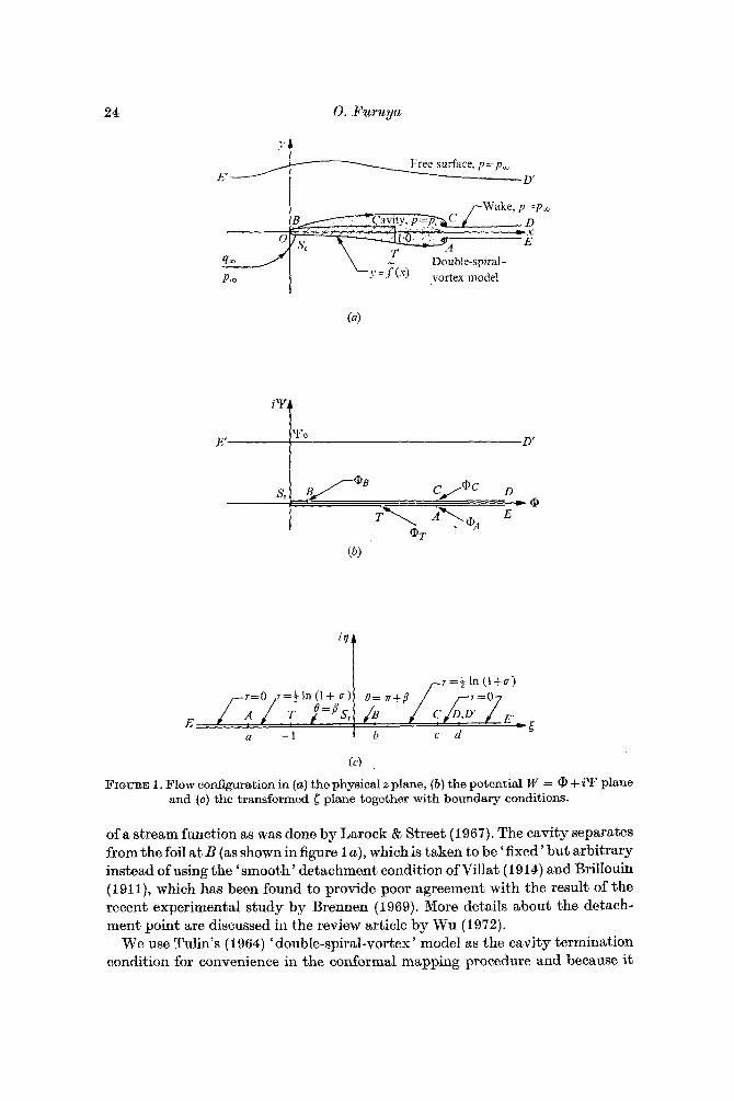
(4 FIGURE 1. Flow codguration in (a) the physical z plane, ( b ) the potential W = @ +iy plane

and (6) the transformed 6 plane together with boundary conditions.

of a stream function as was done by Larock & Street (1967). The cavity separates from the foil at B (as shown in figure 1 a), which is taken to be 'fixed ' but arbitrary instead of using the 'smooth' detachment condition of Villat (1914) and Brillouin (1911), which has been found to provide poor agreement with the result of the recent experimental study by Brennen (1969). More details about the detach- ment point are discussed in the review article by Wu (1972).

We use Tulin's (1964) 'double-spiral-vortex ' model as the cavity termination condition for convenience in the conformal mapping procedure and because it

Arbitrarily shaped supercavitating hydrqfoils 25

't

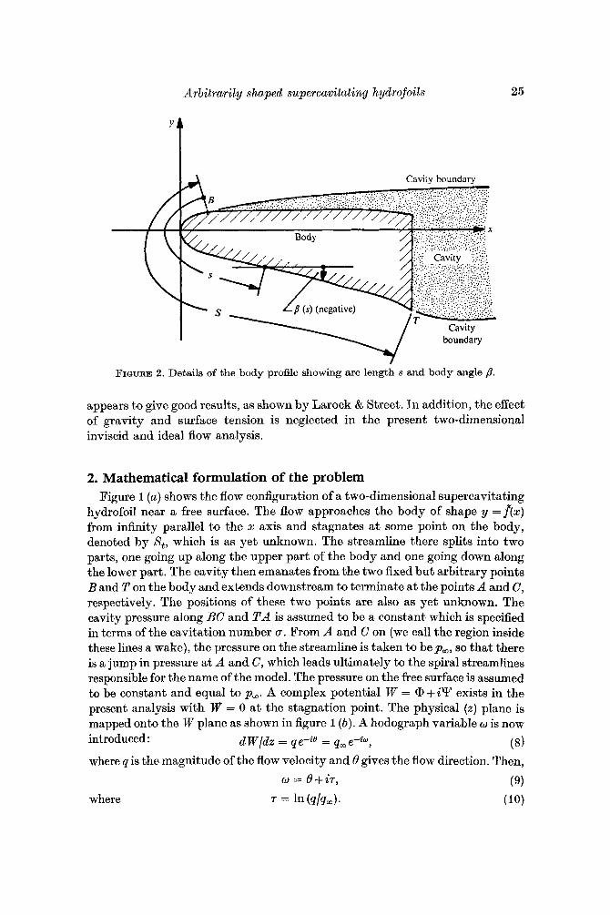
FIGURE 2. Details of the body profile showing arc length s and body angle /3.

appears to give good results, as shown by Larock & Street. In addition, the effect of gravity and surface tension is neglected in the present two-dimensional inviscid and ideal flow analysis.

2. Mathematical formulation of the problem Figure I (a) shows the flow configuration of a two-dimensional supercavitating

hydrofoil near a free surface. The flow approaches the body of shape y = f ( x ) from infinity parallel to the x axis and stagnates a t some point on the body, denoted by S,, which is as yet unknown. The streamline there splits into two parts, one going up along the upper part of the body and one going down along the lower part. The cavity then emanates from the two fixed but arbitrary points Band T on the body and extends downstream to terminate a t the points A and C, respectively. The positions of these two points are also as yet unknown. The cavity pressure along BC and T A is assumed to be a constant which is specified in terms of the cavitation number (T. From A and C on (we call the region inside these lines a wake), the pressure on the streamline is taken to bep,, so that there is a jump in pressure at A and C, which leads ultimately to the spiral streamlines responsible for the name of the model. The pressure on the free surface is assumed to be constant and equal to p,. A complex potential W = CD + iY exists in the present analysis with W = 0 a t the stagnation point. The physical ( 2 ) plane is mapped onto the W plane as shown in figure 1 ( b ) . A hodograph variable w is now introduced :

where q is the magnitude of the flow velocity and 8 gives the flow direction. Then, d Wldz = q r i s = qm e-iw, (8)

where

26 0. Turuya

All boundary conditions can be expressed in terms of either the real or imaginary part of o, forming a so-called mixed boundary-value problem. On the body between St and T (see figure 2)

% = p, where tanp = dfldx, (11 a ) y = f(x) defining the wetted surface of the foil. Between S, and B

e = ~ + n . On the cavity boundaries

7 = +1n(1 +g),

where the Bernoulli equation has been applied between the point a t infinity and that on the cavity boundary. Finally, on the wake and free surface

7 = 0. (11 4 Yo in figure 1 (b) , specified in the present problem, is a parametric representation for the submergence and physically denotes the total flow rate between the free surface and the streamline passing through the stagnation point. All the other co-ordinates QA, QT, QB and Qc are as yet unknown, and incidentally never appear directly in the present calculations. For simplicity we arbitrarily assume that

which was also used by Larock & Street (1967).

@A = @c, (12)

The W plane is then mapped onto the upper half of a new 5 plane by the mapping function w = -3 nd ( < + d l n F ) -d '

where d is the 6 co-ordinate corresponding to the points D and D' at downstream infinity. Since the scaling of the mapping is arbitrary, we take the 5 co-ordinate of the point T to be - 1. All the other co-ordinates a, ..., d in figure 1 ( c ) are as yet unknown parameters to be determined by various boundary conditions. One of these is given by (12) and is

fi f (a+dlna-d) - a -

Three more equations will be provided by imposing the boundary conditions at infinity and the scaling condition between the physical and transform planes on the solution of the boundary-value problem.

The boundary conditions on the real-5 axis of the 6 plane are now expressed as

7 = {OJ - m < $ < a , c < E < o o , (15 a)

+ l n ( l + n ) , a < .i< - 1 , b < .$< c , ( 1 5 b )

(15 c)

= O < [ < b . (15 4 - 1 < ( < 0,

By analytically continuing ~ ( 6 ) into the lower half < plane by the reflexion principle w(5*) = o*(5), (16)

Arbitrarily shaped supercavitating hydrofoils 27

where * denotes a complex conjugate, we can write

The boundary conditions (15) are now expressed in the form

2iT(6,0) = 0, -a < < < a, c < 6 < 00, (18a) 2 i ~ ( < , 0) = i ln ( I + (T), (18 b ) a < 5 < - 1, b < < < c,

W+-@- =

The homogeneous problem corresponding to the present one is described by

H+-H-=O, - 0 0 < c < - I , b < ( < w , (19a) H++H-=O, - I < ( < b , ( 1 9 b )

where H(C) is a homogeneous solution. By inspection H ( [ ) can be easily found to be

taking into account the condition that no singularities are allowed a t the upper and lower separation points. We choose a branch cut for H($ such that

H- = - [($+ 1) (<-b)]4 (31 a )

H(C) = [(5+ 1 ) (C-b)I+, (20)

-00 < ,g < - 1, - H - = i [ ( I + g ) ( b - < ) ] * , - I < $ < b, (21 b )

H- = [(<+ 1) (<-b)14 b < [ < c o . (21 c )

Introducing a new function G(C) defined by

G(C) = w(C)/H(CL we finally can write (1 8) in terms of G+ - G- as follows:

~H+-l(w+ - W - ) = 0, -XI < ( < a, ( 2 3 ~ ) H+-l(w+-w-) =- i ln( I+a) / [ ( (+ l ) ( t -b) ]~ , a < $ < -1, (23b)

H+-l(w+ + w-) = 2/3/i[( 1 + E ) (b - 5)]4 ( 2 3 ~ ) H+-l(w++w-) = ( 2 / 3 + 2 ~ ) / i [ ( I + ( ) ( b - 6 ) ] * , 0 < c < b, ( 2 3 d )

- 1 < < < 0,

H+-l(wf-w-) = i l n ( l + ( ~ ) / [ ( ~ + l ) ( ~ - - b ) ] * , b < 6 < c, (23e ) iH+--l(w+ - w-) = 0, c < E < 00. ( 2 3 f )

The application of Plemelj's formula (see, for example, Carrier, Krook & Pearson 1966) yields the general solution

28 0. Hwuya

It should again be mentioned that the angle of the body P in the second integral of (24) is not known a priori as a function of 5, so that this integral cannot be evaluated explicitly except for a flat plate, in which case /3 is constant.

The boundary conditions which have not yet been used are those at infinity:

Im (w( .o)} = Im (o(d)} = 0. (25 a, b) Applying (25 ) to w in (34), we obtain

- ( b + 1 ) f 2 = 2T + 4 (In 2[(a + 1) (a - b)]&+ (a + 1 ) + (a - 6 )

I b + l 2[(c+ I) (c - b)]4+ (c 4- 1) + (c - 6 ) + In

and ( I + b ) ( a - d )

f 3 = In(' 27T +g)(ln 2 1 ( ~ + I) (a -b ) (d + I ) (d - b ) ] f + (a+ 1) (d - b ) + (a - b ) (d + 1)

(1 +b) (d - c) 2[(c+ I) ( c - b ) (d+ 1)(d-b)]++ (c + 1) ( d - b ) + (c- b ) (d+ 1) f In

(27) The final equation will be obtained by the scaling between the transformed

potential and physical planes. Defining s t o be the arc length of the wetted part of the foil measured from the point B as depicted in figure 2, we can express the co-ordinates of the body parametrically as

x = x(s ) , y = y(s), 0 < s < 8, (28)

where S denotes the total arc length of the wetted portion. Then the inclination p of the body is given by

Since on the body surface

then

dz/ds = eiP, dz dW

Using the relations (8) and (13), we can write (31) as

w ( E ) for - 1 < 6 < b is found to be, from (24),

Arbitra,rily shaped supercavitating hydrofoils 29

where $ means the Cauchy principal value of the improper integral, and In ( - 1) is taken to be -in. Substitution of the above equation for w ( g ) into (32a)

s(k-) = - - provides

where

hG, a7 b, C) = exp { - Im ( ~ ( c ) ) } ,

a’, a, b, c ) w, d, Yo) d5‘, (32 b) S b 5

- 1 < 5 < b,

Now the proper scaling can be achieved by requiring

f 4 = s( - I ) - As = 0. (34) This now completes a system of four nonlinear equations fl, . . . ,f4 = 0, given in (14), (26), (27) and (34), respectively, for the four unknown parameters a, ..., d.

3. Numerical method The system of four nonlinear equations f = 0 can now be solved for the solution

parameters a = (a, b, c, d ) by following the iteration procedure in (7). Starting values of ,8 and a (providing the ‘basic ’ flow) are to be chosen to initiate Newton’s iterative loop with v = I and n = 1 in (7); two different types of basic flow may be considered, one being that for a flat plate, in which p is chosen to be constant and a is guessed by experience, and the other any similar flow which has already been obtained, perhaps as a result of previous numerical work. It is noted that the first starting value p1 may have nothing to do with the actual body angle ~3 specified as part of the problem although one tries to choose B1 as close to ,!3 as possible. With B1 and ail) chosen, the values off and J t can now be found because the integrals in (26), (27) and (34)$ involving /3 may be evaluated. Now (7) is a system of linear equations for ai2) - ail) with all coefficients known, so that ai2) can easily be found. We then proceed to the next iteration loop of Newton’s method to find aI3) by using the ai2) just obtained and using the same B1 and so on.§

t Most of the partial derivatives in J may be obtained numerically, for J is always regular its long as a is close to its exact form.

$ Incidentally, if /3 is expressed as any polynomial in 6, these integrals have closed forms; if ,8 is a constant, they are -PT, - / 3 ~ / [ ( d + 1) (d- b)]* and zero, respectively.

§ During each iteration loop of Newton’s method (1% = 1, 2, . . .) the range of ,8,([) must be changed from - 1 < E < bl]) to - 1 < [ < b?) so that the same value /3,([) can be used although b, changes from one iteration to another. One way of doing this is to redefine .&(E) ssP,( t ) , where t = - l + { ( l + b ~ ’ ) / ( l + b ~ ’ ) ) ( l + E ) .

30

8JO Newton's method, equations.

Y * 4 (14). (26). (27L (34) a"'

where v =I

0. Furuya

From equation (376)

a r n t l ) Y U G v f l

solution i n - B ( " , ( E ) converged

a"'- ( " + I ) Newton's =a method Y - I

I I Starting solution

FIGURE 3. A schematic iterative loop of the numerical procedure.

With a converged set of we now have a direct although approximate relationship between < and s through (32 b ) . This relationship is now used to determine the next approximation /3&) by substituting the approximate func- tion s(<) into the actual body-angle distribution P(s); the body-angle distribution is sketched in figure 2. We now have completed one loop of the functional iterative method, that for v = 1. Renaming the converged solution parameter a:m+1) as ail) for v = 2 and usingPz((), we repeat the same procedure and continue for v = 3 , 4 , ..., until a convergent solution is obtained. It is noted that P,(() must converge as well as a. The schematic diagram shown in figure 3 summarizes the whole iterative procedure.

4. Some basic characteristics of the flow 4.1. Pressure distribution, lift and drag

The pressure distribution on the foil is expressed here in terms of a pressure coefficient defined by

c, = (P - P,) / iP6, (35)

where qc is the magnitude of the flow velocity on the cavity boundaries. Applying the Bernoulli equation a t upstream infinity and on the body surface, we can write (35) as

Since q is given by (8), c, = l-q"(l+Gqq2,. (3Ga)

4 = 4 m exp(Im [ 4 E ( W I } , - 1 < c < b,

and also w(<) has been given for - 1 < ( < b, C, is finally found to be given by

CJE(4, = 1 - 1/(1 + 4 {W(Z), a, b, C ) y , (36 b )

where h(<(x), a, b, c) is defined in (33 a) .

taken to be unity, can now be obtained in the combined form Lift and drag coefficients CL and CD normalized by the foil length, which was

Arbitrarily shaped supercavitating hydrofoils 31

where dxlds and dsldc' are given by (30) and (32b) . Therefore, P h

where k is given in (33 b ) . It is noted that C, and C, are defined here with respect to q, instead of qm, so that 'conventional' force coefficients can be obtained by multiplying CL and C, by the factor 1 + cr.

4.2. Cavity and free-surface shapes The streamline shape is obtained by integrating (8):

where the subscript r denotes reference points in the z or (5 plane. The upper cavity shape is then given by

where zB = xB + iyB is the complex co-ordinate of the upper separation point B. w ( g ) for b < 5 < c is obtained from (24):

o([) = Rew,+iImw,, b < E < c,

where

Re %(El ) - (1+b) (a -C) ln( l+r)( ln 27T

2 [ ( a + 1 ) (a- b ) (1 +5) (5- b ) @ + (a+ I) ( 5 - b ) + (a - b ) (1 +5) -

Imw, = f r ln( l+a) .

Therefore, in component form,

y-yB = - exp{-Imw,}sin{Rew,(~)}k(~,d,Yo)d~, b < 6 < c , ( 4 2 b ) qa s' b

where it is noted that x and y are expressed through a parameter 5.

32 0. Furuya

Similarly the lower cavity shape is given by

5 x-+ = - 1 exp { - Im q) cos {Re ~~(5 ' ) ) k(g', d, Yo) dg', a < 5 < - 1, (43 a) Pa3 -1

y-yT = ~/~lexp{-Imo,}sin{Rew,(~)}k(~,d,Yo)d~', a < 5 < -1, (43b)

where (xT, yT) are the physical co-ordinates of the lower cavity separation point T. Re wl and Im wl are the real and imaginary parts of w ( g ) for a < 5 < - 1, which are again obtained from (24) :

Re Y(5) - (1 +b) ( 5 - a )

In ( l + 27r a) (In 2[(1 +a) (a - b ) (1 + 5) (6 - b)]* + (a + 1) (5 - b) + (a - b ) (1 + 5) - -

I (1 + b ) G - C )

2[(1 + G ) ( G - b ) (1 +5) (t-b)]* + (c+ 1) (5- b) + (c -b) (1 +g) + In

Imw, = &ln( l+a ) .

The free-surface shape is found as before:

1 5 x - xc = -Ic exp ( - Im wf} cos (Re w f ( F ) } k ( g , d, Yo) dg, c < 5, (45 a)

Y -Yc = -Jc exp { - I m q} sin {Re w&')} k ( r , d, Yo) dy, c < <, (45 b)

qa

q m

where (xcJ yc) are the co-ordinates in the z plane corresponding to the upper end of the cavity. Also,

Re Wf(5)

- - ( 1 + b ) (a - 6) 27r

In + a) (In 2[(a + 1 ) (a - b ) ( 1 + 5) (g - b)l* + (a + 1 ) (g - b ) + (a - b ) ( 1 + 5)

(1 + b ) ( 5 - c ) 2[(c+ 1) ( c - b ) (1 +t) (<--b)l*+ ( c+ 1) ( 5 - b ) + ( c - b ) (1 +5) + In

Imwf= +In ( l+a ) .

At the end points A and C of the cavity, the numerical calculations of the cavity shape must be carried out taking g in (43) or (40) not identically equal to a or c because of the logarithmic singularities. Also a t the point D or D', which corresponds to that on the upper wake or on the free surface at downstream infinity, the original integral (39) instead of (45) is to be evaluated by substituting 5' = d + 8 e i y , retaining 6 very small but not zero and varying y from 7r to 0

Arbitrurily shmped supercavituting hydrqfoils 33

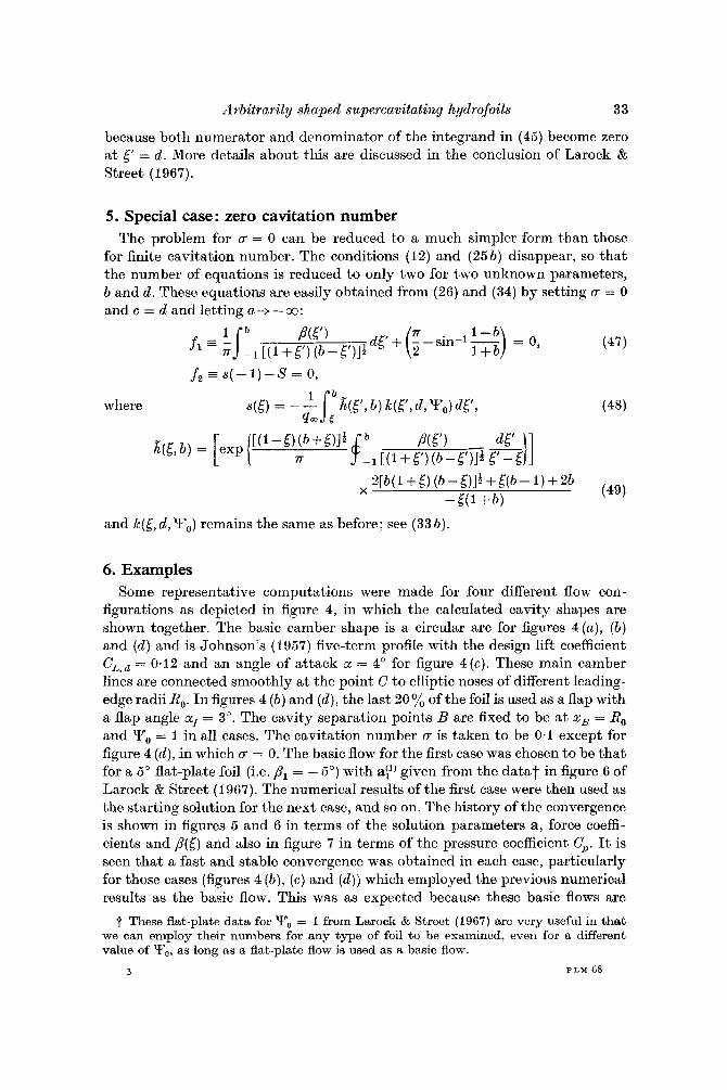
because both numerator and denominator of the integrand in (45) become zero a t = d. More details about this are discussed in the conclusion of Larock & Street (1967).

5. Special case: zero cavitation number The problem for u = 0 can be reduced to a much simpler form than those

for finite cavitation number. The conditions (12) and ( 2 5 b ) disappear, so that the number of equations is reduced to only two for two unknown parameters, b and d . These equations are easily obtained from (26) and (34) by setting u = 0 and c = d and letting a+-co:

where

fi = s( - 1 ) -8 = 0,

(49) 2[b( 1 +() (b - &')]a +((b - 1 ) + 2b

X - 5 ( 1 + b )

and k ( 6 , d , Y o ) remains the same as before; see (33 b) .

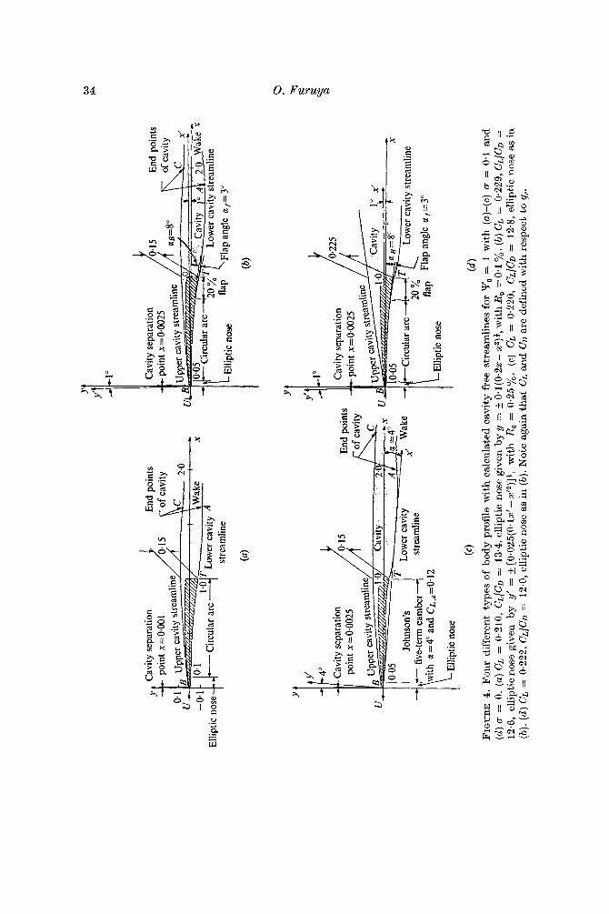
6. Examples Some representative computations were made for four different flow con-

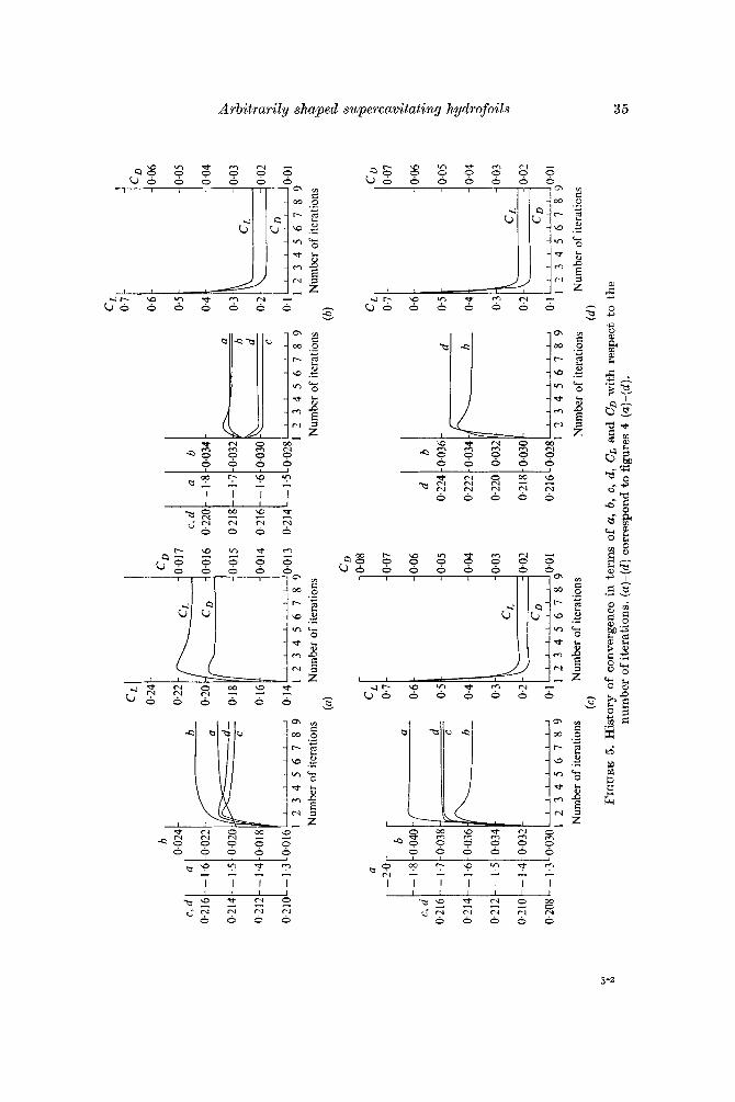
figurations as depicted in figure 4, in which the calculated cavity shapes are shown together. The basic camber shape is a circular arc for figures 4 ( a ) , ( b ) and (d ) and is Johnson's (1957) five-term profile with the design lift coefficient CL,d = 0.12 and an angle of attack a: = 4" for figure 4(c). These main camber lines are connected smoothly a t the point C to elliptic noses of different leading- edge radii R,. I n figures 4 ( b ) and (d) , the last 20% of the foil is used as a flap with a flap angle af = 3". The cavity separation points B are fixed to be a t xB = R, and Yo = I in all cases. The cavitation number u is taken to be 0.1 except for figure 4 (d), in which u = 0. The basic flow for the first case was chosen to be that for a 5" flat-plate foil (i.e. P1 = - 5") with ail' given from the data? in figure 6 of Larock & Street (1967). The numerical results of the first case were then used as the starting solution for the next case, and so on. The history of the convergence is shown in figures 5 and 6 in terms of the solution parameters a, force coeffi- cients and P(6) and also in figure 7 in terms of the pressure coefficient C,. It is seen that a fast and stable convergence was obtained in each case, particularly for those cases (figures 4 ( b ) , ( c ) and ( d ) ) which employed the previous numerical results as the basic flow. This was as expected because these basic flows are

7 These flat-plate data for Yo = 1 from Larock & Street (1967) are very useful in that we can employ their numbers for any type of foil to be examined, even for a different value of Yo, as long as a flat-plate flow is used as a basic flow.

3 F L M 68

Y‘t ’I

Yt

Yt

U

(4

(d )

FIG

UR

E

4. F

our

diff

eren

t ty

pes

of b

ody

prof

ile w

ith

calc

ulat

ed c

avit

y fr

ee s

trea

mli

nes

for

Yo

= 1 w

ith

(a)-

(c) v =

0.1

and

(d

) u =

0.

(a) C

r, =

0.2

10,

CL/

CD

= 1

3.4,

ell

ipti

c no

se g

iven

by

y =

i- 0.

l(0.

2z-z

2)~

, wit

h R

, =

0.1

%. (

b) C

L =

0.2

29, C

L/C

D =

12.6

, el

lipt

icno

se g

iven

by

y’ =

k[O

*025

(0.1

z’-z

’2)]

~, w

ith

R, =

0.2

5%.

(c)

CL

= 0

.220

, C

L/C

D = 1

24

, ell

ipti

c no

se a

sin

(b

). (d

) CL

= 0

.222

, CL/

CD

= 1

2.0,

ell

ipti

c no

se a

s in

(b)

. Not

e ag

ain

that

CL

and

CD

are

defi

ned

wit

h re

spec

t to

qc.

P

c, d

0.21

6--

0.21

4

0,21

2

0210

--

b

1.4 -

0.01

8

I .6

-0.0

22

I .5 -0

.020

1.3 -

0.01

6 12

34

56

78

9

- -

- -

cLI

I - -2

.0-

0.7

-

--1.

8-0,

040

0.6

-

0.5

-

0.4

-

0.3

-

0.2

-

a C

L

CL

CD

0.1 i

c, d

0'

216-

- 1.

7-0.

038

0.21

4--1

.6-0

.036

0.21

2 - - 1.

5 -0.

034

0~21

0--1

+0.0

32

0.20

8 - -

1.3 -

0.03

0

0.01

6

0.18

0.

015

0.16

0,

014

0.14

0.

013

12

34

56

78

9 0.08

0.07

0.06

0.05

0.04

0.03

0.02

12

34

56

78

9

dl

bl

0.

224

0.22

2

0.22

0

0.21

8

0.21

6

0.7

CD

0.06

0.05

0.04

0.3

0.03

0.02

0.

2

0. I

0.0 I

1

23

45

67

89

~~

,,

,~

~,

,~

Num

ber o

f ite

ratio

ns

Num

ber

of i

tera

tions

(b

)

-0.0

36

.0.0

34

- 0.0

32

-0.0

30

- 0.0

28 1

23

45

67

89

CL

CD

0.

7 4 0.07

0.6 1

4 0.06 0.05

0.04

0.3

0.03

0.2

0.02

LA 0.1 1234567

89

C

D L

_J 0.

01

Num

ber o

f ite

ratio

ns

Num

ber o

f ite

ratio

ns

Num

ber

of it

erat

ions

N

umbe

r of

itera

ticns

(4

(d

1 F

IGU

RE

5

. H

isto

ry o

f co

nver

genc

e in

ter

ms

of a, b

, c,

d,

CL

and

CD

wit

h re

spec

t to

th

e nu

mbe

r of

iter

atio

ns.

(a)-

(@ co

rres

pond

to fi

gure

s 4 (a)-(d).

w

or

36

-2 -

0. Furuya

'* 5 (4

-2 1 - 1.0 -0.5

5 (b)

*Flap3 portion

p W ) t

1st iteration

portion 5 (d 1

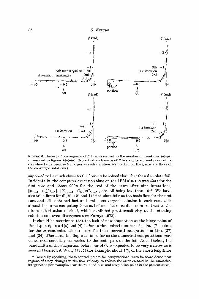
FIGURE 6. History of convergence of p(5) with respect to the number of iterations. (a)-(d) correspond to figures 4 (a)-@). (Note that each curve of /3 hitv a different end point at its right-hand side because b changes at each iteration. b's marked on the 6 axis are those of the converged solutions.)

supposed to be much closer to the flows to be solved than that for a flat-plate foil. Incidentally, the computer execution time on the IBM 370-158 was 530 s for the first case and about 200s for the rest of the cases after nine interations, 11 (av+l - av)/av+l!l, I (CL,y+l - CL,J/CL, v + l l , etc. all being less than We have also tried flows for B", 8", 12" and 14" flat-plate foils as the basic flow for the first case and still obtained fast and stable convergent solution in each case with almost the same computing time as before. These results are in contrast to the direct substitution method, which exhibited great sensitivity to the starting solution and even divergence (see Furuya, 1973).

It should be mentioned that the lack of flow stagnation a t the hinge point of the flap in figures 4 ( b ) and ( d ) is due to the limited number of points (71 points for the present calcu1ations)f used for the numerical integrations in (26), (27) and (34). Therefore, the flap was, in so far as the numerical computations were concerned, smoothly connected to the main part of the foil. Nevertheless, the bandwidth of the stagnation behaviour of C, is expected to be very narrow as is seen in Harrison & Wang (1965) (for example, about 1 yo of the chord length for

t Generally speaking, these control points for computations must be more dense near regions of steep changes in the flow velocity to reduce the error created in the numerica. integrations (for example, near the rounded nose and stagnation point in the present cases)l

Arbitrarily shaped superca,vitating hydrofoils 37

0.002 0,004

near the leading edge

0.5 I .o Circular-arc camber, -AT

El1iptic trailing-edge angle a ~ = 8 '

X T ' LJohnson's five-term camber Elliptic nose with a = 4 " a n d

CL .d= 0.1 2

c. 1.0

CP , 1.0 T (6)

'\ 0.002 0.0025

- l I I I I I , l I

B 10 10.05 0.5 I

trailing-edge angle a0 =8" a,=Y

c, 1.0

x' =I= 4T 20 0; flap

a,=3'

-Circular-arc camber, a ~ = 8 " Elliptic nose

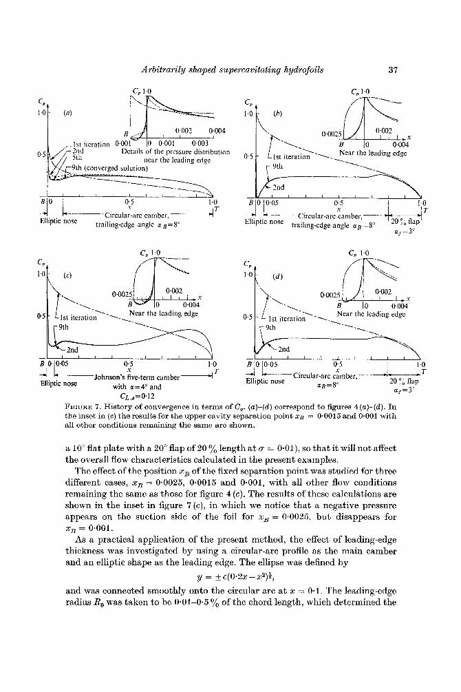
FIGURE 7. History of convergence in terms of C,. (a)-(d) correspond to figures 4(a)-(d). In the inset in (c) the results for the upper cavity separation point 58 = 0-0015 and 0.001 with all other conditions remaining the same are shown.

a 10" flat plate with a 20" flap of 20 yo length a t (T = 0.01)) so that it will not affect the overall flow characteristics calculated in the present examples.

The effect of the position x, of the fixed separation point was studied for three different cases, x, = 0.0025, 0.0015 and 0.001, with all other flow conditions remaining the same as those for figure 4 (c). The results of these calculations are shown in the inset in figure 7 ( c ) , in which we notice that a negative pressure appears on the suction side of the foil for x, = 0.0025, but disappears for XB = 0.001.

As a practical application of the present method, the effect of leading-edge thickness was investigated by using a circular-arc profile as the main camber and an elliptic shape as the leading edge. The ellipse was defined by

y = +e(0.2x-xZ)h, and was connected smoothly onto the circular arc at x = 0.1. The leading-edge radius R, was taken to be 0.01-0.5 yo of the chord length, which determined the

38 0. Fu,ruya

0.1 0.2 0.3 CL = s ( p -pc)dx/+pq: x chord

FIGURE 8. The effect of leading-edge radius on CL/CD vs. Cl, for circular-arc foils as function of trailing-edge camber angle with = 0.1 and Yo = 1. Note that the broken lines show the appearance of negative pressures on the pressure side of hydrofoils. (It is noted that the diagrams of the flow configuration in this figure and in figure 9 are schematic.)

parameter B in each case. In figure 8 the lift-to-drag ratio C,/C, is plotted vs. the lift coefficient C, as function of R, and the trailing-edge angle. As may be clearly seen, the values of C,lC, for the same C, decreased by factors of more than 1-8 from R, = 0.01 % to R, = 0.5 %. Of course, it is well known that, the sharper the leading edge, the better is the hydrodynamic performance obtained. In any case the final choice of R, must be dependent upon practical and structural considerations not within the scope of the present work.

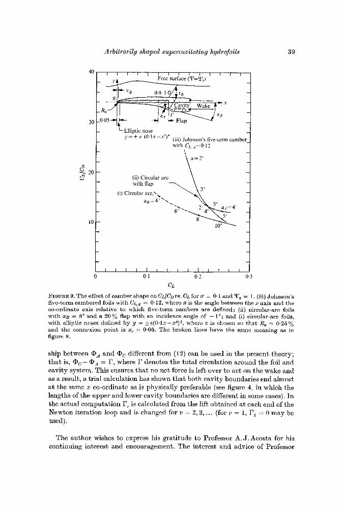
Figure 9 shows C,lCD as function of C, for three different types of camber profile in which the leading edge was represented by an ellipse with R, = 0.25 %. Both the circular-arc foil with a 3" flap and Johnson's five-term camber foil with c,, = 0.12 and a = 4" gave almost the same value of CLlCD, namely about I 2 for C, = 0.23. Incidentally, the distance between the trailing edge of the foil and the upper cavity boundary at the same x co-ordinate (important for practical foil design) was found to be 15 yo of the chord length in each case.

Finally, it may be worthwhile to mention that a new (possibly better) relation-

Arbitrarily shaped supercavitating hydrofoils 39

0 0.1 0.2

CL 0.3

FIGURE 9. The effect of camber shape on CL/CDVS. CL for v = 0.1 and Yo = 1. (iii) Johnson's five-term cambered foils with C L , ~ = 0.12, where OL is the angle between the x axis and the co-ordinate axis relative to which five-term cambers are defined; (ii) circular-arc foils with OLB = 8" and a 20 yo flap with a n incidence angle of - lo; and (i) circular-arc foils, with elliptic noses defmed by y = ie(O*1.z-x2)~, where E is chosen so that R,, = 0.25% and the connexion point is x,. = 0.05. The broken lines have the same meaning as in figure 8.

ship between @ A and Qc different from (12) can be used in the present theory; that is, QQ- @ A = I?, where I? denotes the total circulation around the foil and cavity system. This ensures that no net force is left over to act on the wake and as a result, a trial calculation has shown that both cavity boundaries end almost a t the same x co-ordinate as is physically preferable (see figure 4, in which the lengths of the upper and lower cavity boundaries are different in some cases). In the actual computation rv is calculated from the lift obtained a t each end of the Newton iteration loop and is changed for 1' = 2,3 , ... (for 1' = 1, I?l = 0 may be used).

The author wishes to express his gratitude to Professor A. J.Acosta for his continuing interest and encouragement. The interest and advice of Professor

40 0. Fwuya

T.Y.Wu is also appreciated. This work was supported by the Naval Ship Systems Command General Hydromechanics Research Program, technically administered by the Naval Ship Research and Development Center under Contract N00014-67-A-0094-003 1.

R E F E R E N C E S

ACOSTA, A. J. 1973 Hydrofoils and hydrofoil craft. Ann. Rev. Fluid Mech. 5, 161-184. BRENNEN, C. 1969 Cavitation State of Knowledge. A.S.M.E. BRILLOUIN, M. 1911 Ann. Ch,im. Phys. 23, 145-230. BRODETSKY, S. 1922 Discontinuous fluid motion past circular and elliptic cylinders. Proc.

CARRIER, G., KROOK, M. & PEARSON, C. 1966 Pumtions of a Complex Variable, p. 414. McGraw-Hill.

FURUYA, 0. 1973 Numerical computations of supercavitating hydrofoils of parabolic shape with Wu and Wang’s exact method. California Inst. Tech. Rep. E-79A.15.

FURUYA, 0. & ACOSTA, A. 1973 A note on the calculation of supercavitating hydrofoils with rounded noses. J . Fluids Engng, Trans. A.S.M.E. 95, 222-228.

GILBARG, D. 1960 In Handbuch der Physik, vol. 9, pp. 311-445. Springer. HARRISON, Z. & WANG, D. P. 1965 Evaluation of pressure distribution on a ca,vitat,ing

ISAACSON, E. & KELLER, H . 1966 Analysis of Numerical Method, pp. 113-123, 386. Wiley JOHNSON, V. 1957 Theoretical determination of low-drag supercavitating hydrofoils and

their two-dimensional characteristics a t zero cavitation number. N.A.C.A. Rep. RML57G l l a .

LAROCK, B. & STREET, R . 1967 Nonlinear solution for a fully cavitating hydrofoil beneath a free surface. J . Ship Res. 11, 131-140.

LaROCK, B. & STREET, R. 1968 Cambered bodies in cavitating flow - a nonlinear analysis and design procedure. J . Ship Res. 12, 1-13.

LEVI-CIVITA, T. 1907 Scie e leg@ di resistenzia. R. G. cir. mat., Palermo, 18, 1-37. LURYE, J. 1966 Numerical aspects of Wu’s method for cavitated flow, as applied to

sections having rounded noses. Rep., Melville, N . P., TRG-156-SR-3. MILNE-THOMSON, L. 1968 Theoretical Hydrodynamics, p. 338. Macmillan. MURAI, H. & KINOE, T. 1968 Theoret.ica1 research on blunt-nosed hydrofoil in fully

TULIN, M. 1953 Steady two-dimensional cavity flows about slender bodies. Navy Dept.,

TULIN, M. 1964 Supercavitating flows - small perturbation theory. J . Ship Res. 7, 16-37. VILLAT, H. 1914 Sur la validit6 des solutions de certains problemes d’hydrodynamique.

Wu, T. Y . 1972 Cavity and wake flows. Ann. Rev. Fluid Mech. 4, 243-284. WU, T. Y . & WANG, D. P. 1964 A wake model for free-streamline flow theory. Part 2.

Cavity flows past obstacles of arbitrary profile. J . Fluid Mech. 18, 65-93. YIM, B . 1964 On a fully cavitating two-dimensional flat plate hydrofoil with non-zero

cavitation number near a free surface. Hydronautics Tech. Rep. no. 463-464.

ROY. SOC. A 102, 542-553.

hydrofoil with flap. California Inst. Tech. Rep. E133.1.

cavitating flow. Rep. Inst. High Speed >Tech., Japan, no. 20.

Washington, D.C., D.T.M.B. Rep. no. 834.

J . Math. 10 (6), 231-290.