Nonlinear behaviour of Offshore Flexible Risers …College of Engineering, Design and Physical...
151
College of Engineering, Design and Physical Sciences Department of Mechanical, Aerospace and Civil Engineering A thesis submitted for the degree of Master of Philosophy Nonlinear behaviour of Offshore Flexible Risers Supervisors: Professor Hamid Bahai Dr. Giulio Alfano By: Shayan Norouzi
Transcript of Nonlinear behaviour of Offshore Flexible Risers …College of Engineering, Design and Physical...

College of Engineering, Design and Physical Sciences
Department of Mechanical, Aerospace and Civil Engineering
A thesis submitted for
the degree of
Master of Philosophy
Nonlinear behaviour of Offshore Flexible Risers
Supervisors:
Professor Hamid Bahai
Dr. Giulio Alfano
By:
Shayan Norouzi

ii
Dedicated to
My parents, my sibling, and Sara

iii
Abstract
As the search for exploration of oil and gas moves to deeper waters, flexible unbounded
risers have become the main means of extracting hydro carbonates from deep waters. In
this context, structural integrity of flexible risers has become a crucial issue for the offshore
industry.
In this study, experimental tests and detailed finite element analyses were carried out on a
scaled down model of a flexible riser pipe. The model used consists of four layers which
include two cylindrical polycarbonate tubes and two steel helical layers. One helical layer
represents the carcass layer in an actual flexible riser whilst the other represents the riser
tendon armour layers, wounded around the pipe assembly.
The model was first subjected to a three point bending load in order to study its bending-
curvature behaviour experimentally. Then, the specimen was tested under compressive load
with different pressure values to investigate the effect of pressure on the pipe deformation.
Additionally, the effects of pure axial load and pure pressure with no load on the model were
examined. The effects of static load on the deformation of a single helical tendon layer and
creep behaviour (Shetty, 2013) of the layer were also studied.
The investigation of a single tendon under axial load using finite element based software
shows residual strains results are in good agreement with the experiments. The numerical
model also shows a non-linear behaviour in bending-moment curvature for flexible pipe
which is in a good agreement with the experimental data.

iv
Declaration
This thesis is written based on the research carried out in Brunel University London in United
Kingdom. No part of it has been submitted elsewhere for any other qualification or degree. It
is all my own research except some sections which the works of others were used and the
related authors’ names are mentioned in references.
Copyright © 2014 by Shayan Norouzi.
All right of this thesis are reserved for the author. No quotation from this work is permitted
to be published without his personal signature. If data derived from, it is better to be
acknowledged.

v
Acknowledgements
The author tends to thank his supervisors, Professor
Hamid Bahai and Dr. Giulio Alfano for their helpful
recommendations and guidance during the research
process.
Also thanks to Mr. Keith Withers, whose guidance and
ideas helped a lot to improve the experiments, the
previous researchers of offshore engineering, the staff
of mechanical engineering workshop, and the other
related staff of Brunel University.

vi
Contents
Abstract …………………………………………………………………………………...... iii
Declaration …………………………...………………………………………………….…. iv
Acknowledgements …………………………………………………...………………….... v
Contents …………………………………………...………………………….……………. vi
List of figures …………........................................................................................…… ix
List of tables ……………...................................................................................…… xvii
List of symbols ……………………………………………………………..……………. xviii
1 Introduction 1
1.1 Overview .................................................................................................................... 2
1.2 Subsea Risers Configurations..................................................................................... 3
1.3 Flexible Risers Layers ................................................................................................ 4
1.3.1 Carcass ……………………………………………………………………...……….. 6
1.3.2 Internal Pressure Sheath …………………………………………………………… 6
1.3.3 Inner and Outer Liner ………………………………………………..……………… 7
1.3.4 Anti-wear Layer ……………………………………………………………………… 7
1.3.5 Pressure Armour ………………………………………………………….…………. 7
1.3.6 Tensile Armour ………………………………………………………………………. 8
1.3.7 Outer Sheath ………………………………………………………………………… 8
1.4 Failure Causes ........................................................................................................... 9
1.5 Problem Statement …………………………………………………………………...….. 10
1.6 Research Objectives ................................................................................................ 11
1.7 Thesis Outline .......................................................................................................... 11
vii
2 Literature Review 12
2.1 Overview .................................................................................................................. 13
2.2 Analytical Methods ................................................................................................... 13
2.3 Numerical Models ..................................................................................................... 20
2.4 Experiments ............................................................................................................. 27
2.5 Conclusion ................................................................................................................ 29
3 Experiments 30
3.1 Introduction ............................................................................................................... 31
3.2 Prototype Components ............................................................................................. 31
3.3 Strain Gauges .......................................................................................................... 36
3.4 Scorpio ……………………………………………………………………………..……… 38
3.5 INSTRON 8801 Loading Machine …………………………………………………..….. 39
3.6 Tests on Helical Tendon ………………………………………….……………………… 41
3.6.1 Tensile Dead Loading …………………………………………………………...… 41
3.6.2 Creep Circumstances …………………………………………………………...… 43
3.7 Bending .................................................................................................................... 48
3.8 Axial Loading (Compressive) ................................................................................... 56
3.8.1 Pressure Effects with No external Load …………………………………………. 60
3.8.2 Pressure Effects on Displacement-Load Diagrams …………………………..... 63
3.8.3 Effects of External Axial Load (No Internal Pressure) ………………………..... 64
3.9 Conclusion ............................................................................................................... 68
4 Numerical Modelling 69
4.1 Introduction ............................................................................................................... 70

viii
4.2 Geometry of Models ................................................................................................. 70
4.3 Meshing and Element Selection ............................................................................... 72
4.4 Contact ..................................................................................................................... 76
4.5 Load, Boundary Conditions and Remained Controls ............................................... 79
4.6 Solution Methods ...................................................................................................... 81
4.7 Results and Discussion ............................................................................................ 83
4.7.1 Static Dead Loading ……………………………………………………………….. 83
4.7.2 Bending Simulation …………………………………………………………..……. 87
4.8 Conclusion ................................................................................................................ 89
5 Conclusion and Recommendations for Future Work 90
5.1 Conclusions .............................................................................................................. 91
5.1.1 Experiments on the Flexible Pipe ……………………………………...………… 91
5.1.2 Non-linear Finite Elements Methods ……………….……...……………..……… 92
5.2 Recommendations for Future Work ......................................................................... 93
5.2.1 Enhancing of the Prototype ............................................................................. 93
5.2.2 Further Numerical Investigations ..................................................................... 93
5.2.3 Multi-scale Approach ....................................................................................... 94
Bibliography 95
Appendices 99
A Axial (Compression) Test Results 99
B Blueprints and 3D view of Components 121
C Lagrange Multiplier Method Equations 131

ix
List of Figures
Chapter 1
1.1 Flexible Riser Configurations ………………………..………………………………………... 4
1.2 Flexible Riser and its layers 3D view …………………………………….….…………..…… 5
1.3 Flexible Riser and its layers Cross-Section ……………………………….……………...…. 5
1.4 Carcass Profile ……………………………………………………………..………………..…. 6
1.5 Pressure Armour Profile ………………………………………..…………………………..…. 8
1.6 Failure tree of flexible pipe ………………………………………..………………………..…. 9
1.7 Major Incident rate per riser operational year reported to PSA, Norway ……………….. 10
Chapter 3
3.1 Schematic assembly of prototype 3D view…………………………….…………………… 34
3.2 Schematic assembly of bending test 3D view ………………………….………………….. 34
3.3 Schematic assembly of axial test 3D view ………………………………………….……… 35
3.4 Single tendon assembly for dead loading test 3D view ……………………………….….. 35
3.5 Schematic views of Strain gauges positions ………………………..………………….….. 37
3.6 Scorpio applications and their icons …………………………………….…….……………. 38
3.7 INSTRON 8801 …………………………………………………..…………..……………….. 40

x
3.8 Series 8800 Operating Panel ……………………………………………….……………….. 40
3.9 Tendon with two cylinders ………………………………………………………………….... 41
3.10 Hanger components ……………………………………..……………….…………………. 42
3.11 Tendon - Testing …………………….…………………………………………..………….. 42
3.12 Displacement-Load curves [Single Tendon-Static dead loading] ……………..……….. 43
3.13 Tensile Strain-Load curves at gauge 1 [Single Tendon-Static dead loading] ….….….. 43
3.14 Displacement-Time curve [Single Tendon-Creep Curve-1.4 kg] ……………...……….. 44
3.15 Strain-Time curve at SG 1 [Single Tendon-Creep Curve-1.4 kg] ………………....…… 44
3.16 Strain-Time curve at SG 2 [Single Tendon-Creep Curve-1.4 kg] ……………...…….… 44
3.17 Strain-Time curve at SG 3 [Single Tendon-Creep Curve-1.4 kg] ……………........…… 44
3.18 Strain-Time curve at SG 4 [Single Tendon-Creep Curve-1.4 kg] ……………...…….… 44
3.19 Strain-Time curve at SG 5 [Single Tendon-Creep Curve-1.4 kg] ………………....…… 44
3.20 Strain-Time curve at SG 6 [Single Tendon-Creep Curve-1.4 kg] ………………....…… 45
3.21 Strain-Time curve at SG 7 [Single Tendon-Creep Curve-1.4 kg] ……………...…….… 45
3.22 Displacement-Time curve [Single Tendon-Creep Curve-1.6 kg] ……………...……….. 45
3.23 Strain-Time curve at SG 1 [Single Tendon-Creep Curve-1.6 kg] ………………....…… 45
3.24 Strain-Time curve at SG 2 [Single Tendon-Creep Curve-1.6 kg] ………………....…… 45
3.25 Strain-Time curve at SG 3 [Single Tendon-Creep Curve-1.6 kg] ………………....…… 45
3.26 Strain-Time curve at SG 4 [Single Tendon-Creep Curve-1.6 kg] ………….……...…… 46
3.27 Strain-Time curve at SG 5 [Single Tendon-Creep Curve-1.6 kg] ……….………...…… 46

xi
3.28 Strain-Time curve at SG 6 [Single Tendon-Creep Curve-1.6 kg] ……….………...…… 46
3.29 Strain-Time curve at SG 7 [Single Tendon-Creep Curve-1.6 kg] …………….…...…… 46
3.30 Displacement-Time curve [Single Tendon-Creep Curve-1.8 kg] ……………...……….. 46
3.31 Strain-Time curve at SG 1 [Single Tendon-Creep Curve-1.8 kg] ………………....…… 46
3.32 Strain-Time curve at SG 2 [Single Tendon-Creep Curve-1.8 kg] ……………...…….… 47
3.33 Strain-Time curve at SG 3 [Single Tendon-Creep Curve-1.8 kg] ……………........…… 47
3.34 Strain-Time curve at SG 4 [Single Tendon-Creep Curve-1.8 kg] ………………....…… 47
3.35 Strain-Time curve at SG 5 [Single Tendon-Creep Curve-1.8 kg] ……………........…… 47
3.36 Strain-Time curve at SG 6 [Single Tendon-Creep Curve-1.8 kg] ……………...…….… 47
3.37 Strain-Time curve at SG 7 [Single Tendon-Creep Curve-1.8 kg] ……………........…… 47
3.38 Moment as Function of length and middle load ………………………………………….. 48
3.39 Specimen for bending test: displacement transducers positions ………………..…….. 51
3.40 Strain gauge of the helical tendon ………………………………………………………… 51
3.41 Schematic view of load increments versus time …………………………………………. 52
3.42 Specimen for bending test: air valve on the left, and oil components on the right …... 52
3.43 a) step1: deformation measurements, b) step2: Resulted chart, c) Final calculation .. 54
3.44 Moment Curvature [Bending] ………………………………………………………………. 55
3.45 Compressive Strain-Load curve at gauge 1 ………………...……………………………. 55
3.46 Leakage checking at maximum pressure 1 - assembly view …….………..…...………. 57
3.47 Leakage checking at maximum pressure 2 – Pressure gauge at 20bar (maximum) ... 58

xii
3.48 Leakage checking at maximum pressure 3 – Releasing oil ……………..…......………. 58
3.49 Compressive testing for inner tube …………………………………………..…...………. 59
3.50 Strain gauge for metal tendon (Right) and polymer Tubes (Left) …………………..….. 59
3.51 Displacement-Pressure curve [Axial-Outer Tube and Helical Tendon-pure pressure
effects] ……………………………………………………………………………………………… 60
3.52 Strain-Pressure curve at SG 1 [Axial- Helical Tendon-pure pressure effects] ……..… 61
3.53 Strain-Pressure curve at SG 2 [Axial- Helical Tendon-pure pressure effects] ……..… 61
3.54 Strain-Pressure curve at SG 3 [Axial- Helical Tendon-pure pressure effects] ……..… 61
3.55 Strain-Pressure curve at SG 4 [Axial- Helical Tendon-pure pressure effects] ……..… 61
3.56 Strain-Pressure curve at SG 5 [Axial- Helical Tendon-pure pressure effects] ……..… 61
3.57 Strain-Pressure curve at SG 6 [Axial- Helical Tendon-pure pressure effects] ……..… 61
3.58 Strain-Pressure curve at SG 7 [Axial- Helical Tendon-pure pressure effects] ……..… 62
3.59 Strain-Pressure curve at SG 1 [Axial- Outer Tube-pure pressure effects] ………….… 62
3.60 Strain-Pressure curve at SG 2 [Axial- Outer Tube-pure pressure effects] ………….… 62
3.61 Strain-Pressure curve at SG 3 [Axial- Outer Tube-pure pressure effects] ………….… 62
3.62 Strain-Pressure curve at SG 4 [Axial- Outer Tube-pure pressure effects] ………….… 62
3.63 Strain-Pressure curve at SG 5 [Axial- Outer Tube-pure pressure effects] ………….… 62
3.64 Strain-Pressure curve at SG 6 [Axial- Outer Tube-pure pressure effects] ………….… 63
3.65 Strain-Pressure curve at SG 7 [Axial- Outer Tube-pure pressure effects] ………….… 63
3.66 Pressure effect on Load-Displacement [Axial-Inner Tube] …………………………...… 63
xiii
3.67 Pressure effect on Load-Displacement [Axial-Inner Tube] …………………………...… 63
3.68 Pressure effect on Load-Displacement [Axial-Outer Tube and Helical Tendon] …...… 64
3.69 Pressure effect on Load-Displacement [Axial-Outer Tube and Helical Tendon] …..…. 64
3.70 Displacement-Load curve [Axial-no oil-15kN max] ……………………..……..………… 65
3.71 Strain-Load curve at SG 1 [Axial-Inner Tube-no oil-15kN max] ……………..……….… 65
3.72 Strain-Load curve at SG 2 [Axial-Inner Tube-no oil-15kN max] …………………..….… 65
3.73 Strain-Load curve at SG 3 [Axial-Inner Tube-no oil-15kN max] ……………………...… 65
3.74 Strain-Load curve at SG 4 [Axial-Inner Tube-no oil-15kN max] ……………………...… 65
3.75 Strain-Load curve at SG 5 [Axial-Inner Tube-no oil-15kN max] …………………..….… 66
3.76 Strain-Load curve at SG 6 [Axial-Inner Tube-no oil-15kN max] ……………………...… 66
3.77 Strain-Load curve at SG 7 [Axial-Inner Tube-no oil-15kN max] …………………..….… 66
3.78 Strain-Load curve at SG 1 [Axial-Helical Tendon-no oil-15kN max] ………….……..… 66
3.79 Strain-Load curve at SG 2 [Axial-Helical Tendon-no oil-15kN max] ……….........….… 66
3.80 Strain-Load curve at SG 3 [Axial-Helical Tendon-no oil-15kN max] ……...….……...… 66
3.81 Strain-Load curve at SG 4 [Axial-Helical Tendon-no oil-15kN max] ……...….……...… 67
3.82 Strain-Load curve at SG 5 [Axial-Helical Tendon-no oil-15kN max] ……...……..…..… 67
3.83 Strain-Load curve at SG 6 [Axial-Helical Tendon-no oil-15kN max] ……...….……...… 67
3.84 Strain-Load curve at SG 7 [Axial-Helical Tendon-no oil-15kN max] ……...……..…..… 67
3.85 Strain-Load curve at SG1 [Axial-Outer Tube-no oil-15kN max] ……...……...……....… 67
3.86 Strain-Load curve at SG 2 [Axial-Outer Tube-no oil-15kN max] ……...……...……...… 67

xiv
3.87 Strain-Load curve at SG 3 [Axial-Outer Tube-no oil-15kN max] ……...……...……...… 67
3.88 Strain-Load curve at SG 4 [Axial-Outer Tube-no oil-15kN max] ……...……...……...… 67
3.89 Strain-Load curve at SG 5 [Axial-Outer Tube-no oil-15kN max] ……...………....…..… 68
3.90 Strain-Load curve at SG 6 [Axial-Outer Tube-no oil-15kN max] ……...………....…..… 68
3.91 Strain-Load curve at SG 7 [Axial-Outer Tube-no oil-15kN max] ……...……...……...… 68
Chapter 4
4.1 Prototype Layers ............................................................................................................ 70
4.2 Workbench model of prototype for bending ................................................................... 71
4.3 Single Tendon model ..................................................................................................... 71
4.4 SOLID 185 for loading component at bending ............................................................... 73
4.5 SHELL 181 for prototype layers at bending ................................................................... 73
4.6 SURF 154 [Bending] ...................................................................................................... 74
4.7 C3D8R Node Numbering and 1x1x1 integration point scheme ..................................... 74
4.8 Meshing [Bending] ......................................................................................................... 75
4.9 Meshing [Static dead loading] ........................................................................................ 75
4.10 CONTA174 [Bending] .................................................................................................. 76
4.11 Target170 [Bending] ..................................................................................................... 77
4.12 Target170 Segment types [Bending] ............................................................................ 77
4.13 Contact detection point at Gauss point [Bending] ........................................................ 78

xv
4.14 Contact modelling [Bending] ........................................................................................ 78
4.15 Schematic view of the Single Helical Tendon study ..................................................... 79
4.16 ABAQUS modelled load and boundary conditions using References Points [Static dead
loading] …………………………………………….……………………………………………….. 79
4.17 Schematic view of bending .......................................................................................... 80
4.18 ANSYS modelled load, frictionless support, and boundary conditions [Bending] ........ 80
4.19 Deformation at last second [Static dead loading] ......................................................... 83
4.20 Displacement-Load curves ........................................................................................... 84
4.21.a Tensile Strain-Load curves at SG1 [Single Tendon-Static dead loading] ……..….... 84
4.21.b Torsional Strain-Load curves at SG 1 [Single Tendon-Static dead loading] ……...... 84
4.22.a Tensile Strain-Load curves at SG 2 [Single Tendon-Static dead loading] ………..... 85
4.22.b Torsional Strain-Load curves at SG 2 [Single Tendon-Static dead loading] ……...... 85
4.23.a Tensile Strain-Load curves at SG 3 [Single Tendon-Static dead loading] ………..... 85
4.23.b Torsional Strain-Load curves at SG 3 [Single Tendon-Static dead loading] ……...... 85
4.24.a Tensile Strain-Load curves at SG 4 [Single Tendon-Static dead loading] ………..... 85
4.24.b Torsional Strain-Load curves at SG 4 [Single Tendon-Static dead loading] ……...... 85
4.25.a Tensile Strain-Load curves at SG 5 [Single Tendon-Static dead loading] …….….... 86
4.25.b Torsional Strain-Load curves at SG 5 [Single Tendon-Static dead loading] ……...... 86
4.26.a Tensile Strain-Load curves at SG 6 [Single Tendon-Static dead loading] ………..... 86
4.26.b Torsional Strain-Load curves at SG 6 [Single Tendon-Static dead loading] ……...... 86

xvi
4.27.a Tensile Strain-Load curves at SG 7 [Single Tendon-Static dead loading] ………..... 86
4.27.b Torsional Strain-Load curves at SG 7 [Single Tendon-Static dead loading] ……...... 86
4.28 Deformed prototype (total direction) [Bending] ............................................................ 87
4.29 Moment Curvature [Bending] ....................................................................................... 87
4.30.a Compressive Strain-Load curves at SG 1 …………………………….…………..….... 88
4.30.b Torsional Strain-Load curves at SG 1 …………………………………….…………..... 88
4.31.a Compressive Strain-Load curves at SG 2 …………………………………….……...... 88
4.31.b Torsional Strain-Load curves at SG 2 …………………………………………….…..... 88
4.32.a Compressive Strain-Load curves at SG 3 ………………………………….………...... 89
4.32.b Torsional Strain-Load curves at SG 3 ………………………………………….……..... 89
4.33.a Compressive Strain-Load curves at SG 5 …………………………………………….... 89
4.33.b Torsional Strain-Load curves at SG 5 ………………………………………….……..... 89

xvii
List of Tables
3.1 Prototype Dimensions .................................................................................................... 32
3.2 Material data for each layer ............................................................................................ 32
3.3 List of Axial tests (Air Pressure) ..................................................................................... 55
3.4 List of Axial tests (Oil Pressure) ..................................................................................... 55

xviii
List of Symbols
do outer diameter
di inner diameter
E module of elasticity
GF gauge factor
I area moment inertia
L length of beam
M bending moment
Ma bending moment at point A
My yield moment
P bending load
Ra reaction force at point A
Ri inner radius
RG initial resistance of gauge
Rm mean radius
Ro outer radius
Rev Number of revolutions (pitches)
t thickness
x horizontal direction at bending
X bending curvature
y vertical direction at bending
y maximum bending radius
∆R strain made resistance
ϵ strain
Pi number
stress
y yield stress

Chapter 1:
Introduction

Chapter 1 Introduction
2
1.1 Overview
In recent decades, as global oil demand has been rising, oil exploration and production has
been progressing into deeper water. As a result, industrial competition for designing efficient
and reliable facilities to reach the hydro-carbonates in ultra-deep waters in areas such as
Gulf of Mexico, southern shores of Caspian Sea, Norwegian Sea and Greenland waters has
become inevitable. This has led to the rapid development of the flexible risers capable of
functioning in a harsh environment in deeper waters often exceeding 3km below sea level.
One key development has been the unbounded flexible risers used to transport oil and gas
at high internal and external pressure between the seabed and surface in deep waters.
Flexible risers consist of several polymer and steel layers that are, to a certain extent, free to
move internally relative to each other. This gives low bending stiffness and makes them
highly valuable tools for subsea oil and gas companies. Their ability of withstanding against
both horizontal and vertical displacements made them ideal for floating platforms.
Due to the complex geometry of flexible risers, the conventional stress prediction and fatigue
analysis tools based on analytical formulations and linear methods are not adequate.
Instead, detailed non-linear finite element methods or experimental methods are required to
take into account the contact and friction between the layers, radial contraction and
delamination. In this thesis both detailed finite element methods and experimental
techniques are used to analyse the complex structural behavior of flexible risers.
In this chapter, first the main configurations for flexible risers are briefly explained. Then, the
components of a typical flexible riser are described. Finally, the objective, scope of the
research, and outline of the thesis are presented.

Chapter 1 Introduction
3
1.2 Subsea Risers Configurations
As shown in figure 1.1, flexible risers can have the following configurations:
Steep wave,
Lazy wave,
Steep S,
Lazy S.
The first two configurations perform through incorporate buoyancy modules (Tong and Tang,
1997); in these configurations, synthetic foam used to make buoyancy elements which are
connected to the longer length of the pipe; hence, negative weight results to wave shape,
which separates the movements of risers of Touch down point (TDP) from vessel motion.
The steep wave requires a base and a bend stiffener at sea floor and therefore the lazy
wave is more desired; in some projects where internal fluid density changes with life of the
riser, steep wave configurations is a good solution. Buoyancy elements would lose volume if
the pressure is high and submerged weight would increase (Løseth, 2011).
The next two configurations are known as S-configurations in which anchored buoyancy
modulus is used; the buoy component is attached to the pipe and creates an S-shape; it
might either be fixed or floated. Tension variation is absorbed by buoy and minimized at
TDP. S-configurations are expensive because of the infrastructure requirements (Løseth,
2011).

Chapter 1 Introduction
4
Figure 1.1 Flexible Riser Configurations (Løseth, 2011)
1.3 Flexible Risers Layer1
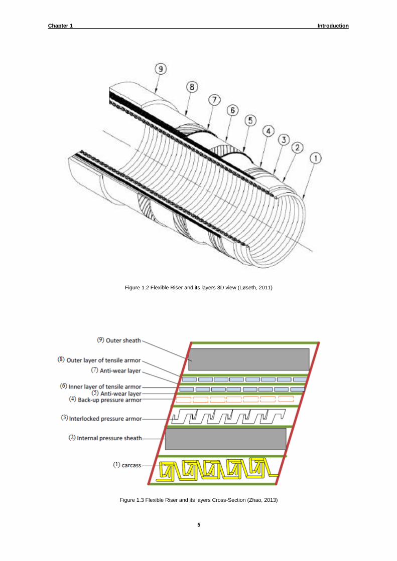
A typical unbounded flexible riser consists of six to twenty layers with different materials and
cross-sections (Løseth, 2011). The layers of a typical flexible riser are shown in figures 1.2
and 1.3.
(1) A detailed discussion upon layers is presented in Bai and Bai (2010).
Chapter 1 Introduction
5
Figure 1.2 Flexible Riser and its layers 3D view (Løseth, 2011)
Figure 1.3 Flexible Riser and its layers Cross-Section (Zhao, 2013)

Chapter 1 Introduction
6
1.3.1 Carcass
An interlocked carcass is the innermost part of the pipe structure; it has an interlocking
cross section with a high lay angle with respect to the pipe longitudinal direction. The profile
of carcass is demonstrated in figure 1.4. Carcass is commonly made from steel AISI 304,
steel AISI 316, or Duplex steel (Løseth, 2011). Its function is to contact with internal fluid
directly in the bore and make resistance against the external pressure. The fluid freely flows
through the carcass in the bore.
Figure 1.4 Carcass Profile (Løseth, 2011)
1.3.2 Internal Pressure Sheath
This layer ensures internal fluid integrity and is used as sealing component; is made from
thermoplastic polymer, either extruded over the carcass or tape wrapped. This layer
guarantees the fluid temperature (Bai and Bai, 2010). The possible material options of
internal pressure sheath have listed below (Zhao, 2013):
Polyamide (nylon), PA11 or PA22
Poly vinylidene fluoride (PVDF)
High density polyethylene (HDPE) and cross-linked polyethylene (XLPE)

Chapter 1 Introduction
7
1.3.3 Inner and Outer Liner
These layers are made from polyethylene (e.g. HDPE, XLPE), or polyamide (e.g. PA11) and
polyvinylidene fluoride (e.g. PVDF). They have the ability to withstand high mechanical and
thermal strains which makes them crucial; the thermal properties of these layers mostly are
defined as design limits (Løseth, 2011).
1.3.4 Anti-wear Layer
The aim of considering this layer in flexible risers is separating metallic armour layers and
therefore reducing the friction. Typically, they are made from polyethylene, polyamide, or
polyvinylidene fluoride (Løseth, 2011).
1.3.5 Pressure Armour
Also called Zeta pressure spiral or flat spiral, this layer has zeta shaped cross-section and
similar to carcass, its lay angle with respect to the pipe longitudinal direction is high (about
89 degree). A typical pressure armour profile is shown in figure 1.5. The zeta shaped profiles
let the layer to bend easily and the gap between armour wires would be controlled; hence,
internal sheath through this layer would not be extruded. This layer is mainly designed for
the applied hoop stresses made from internal pressure; in addition, it can resist against
external pressure, accidental loads, and crushing effects from the tensile armour layer. The
material used for this layer is mainly low carbon steel alloys, which have bigger yielding
strength around 700 to 1000 MPa. Profiles used for pressure armours designs are: Theta
shaped, C-Clip, X-LINKT, and K-LINKT. As a reinforcement, zeta profile might be assembled
by a flatted steel helix (Løseth, 2011 and Zhao, 2013).

Chapter 1 Introduction
8
Figure 1.5 Pressure Armour Profile (Løseth, 2011)
1.3.6 Tensile Armour
Also known as axial armour or helical tendon, this layer consists of two or four cross
wounded layers (pairs), which are made from flat rectangular wires with low lay angle with
respect to the pipe longitudinal direction (30 to 55 degree). This layer provides longitudinal
strength (axial loads) and supports the structure weight by transferring it to the termination
point atop. When axial load is applied, the induced torsion on helical cross wounded layer
can be balanced by using another layer with different angular assembly; hence, the number
of cross wounded in the structure is always even. It also transfers some longitudinal loads to
radial direction similar to the direction of the external pressure. They are made from low alloy
steels with yield points of 700 to 1500 MPa (Løseth, 2011, Zhao, 2013 and Norouzi, 2012).
1.3.7 Outer Sheath
Also known as external thermal plastic layer, this layer is the only visible layer of the flexible
pipe from outside. It has designed for protecting the structure from sea-water intrusion,
corrosion, abrasion, damages during the handling, and binding the armour layers (Zhao,
2013 and Norouzi, 2012).
Chapter 1 Introduction
9
1.4 Failure Causes
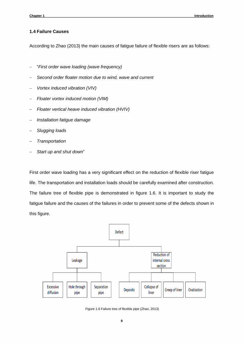
According to Zhao (2013) the main causes of fatigue failure of flexible risers are as follows:
“First order wave loading (wave frequency)
Second order floater motion due to wind, wave and current
Vortex induced vibration (VIV)
Floater vortex induced motion (VIM)
Floater vertical heave induced vibration (HVIV)
Installation fatigue damage
Slugging loads
Transportation
Start up and shut down”
First order wave loading has a very significant effect on the reduction of flexible riser fatigue
life. The transportation and installation loads should be carefully examined after construction.
The failure tree of flexible pipe is demonstrated in figure 1.6. It is important to study the
fatigue failure and the causes of the failures in order to prevent some of the defects shown in
this figure.
Figure 1.6 Failure tree of flexible pipe (Zhao, 2013)
Chapter 1 Introduction
01
1.5 Problem Statement
Even though the importance of using flexible risers for subsea technology in offshore oil and
gas production is well known, the complex structural behaviour of flexible risers is not
sufficiently understood for many design and development purposes. On the one hand
flexible risers must be reliable enough to safeguard the environment. On the other hand,
they must make the exploitation of the subsea hydrocarbons economically feasible. It is clear
that due to ultra-deep water usage, the processes of repairing the risers are very expensive.
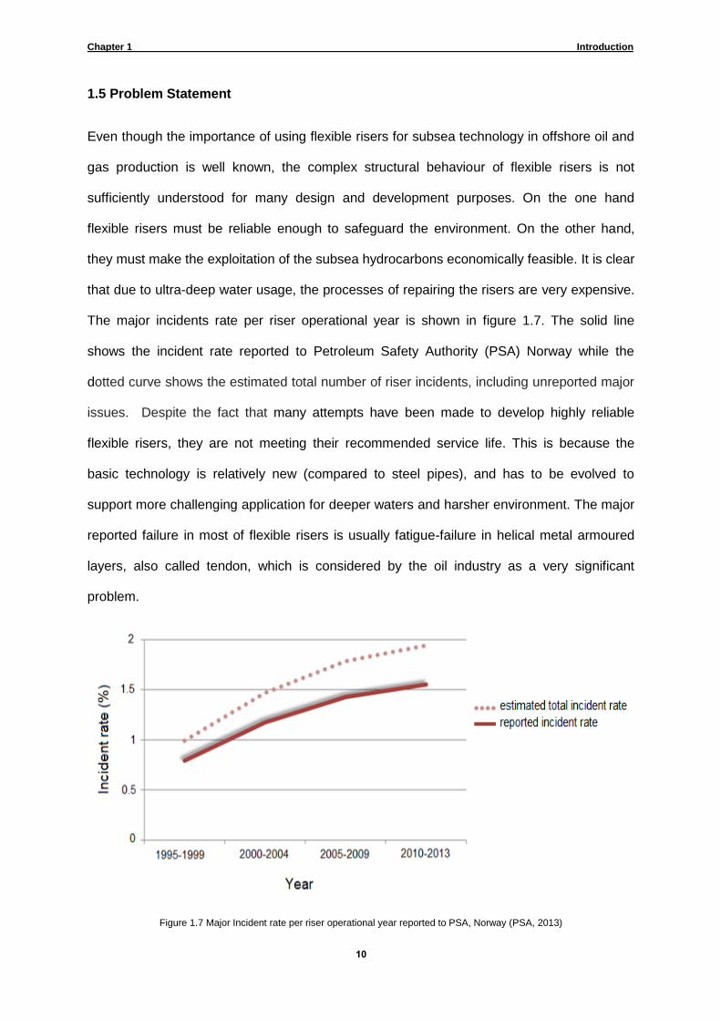
The major incidents rate per riser operational year is shown in figure 1.7. The solid line
shows the incident rate reported to Petroleum Safety Authority (PSA) Norway while the
dotted curve shows the estimated total number of riser incidents, including unreported major
issues. Despite the fact that many attempts have been made to develop highly reliable
flexible risers, they are not meeting their recommended service life. This is because the
basic technology is relatively new (compared to steel pipes), and has to be evolved to
support more challenging application for deeper waters and harsher environment. The major
reported failure in most of flexible risers is usually fatigue-failure in helical metal armoured
layers, also called tendon, which is considered by the oil industry as a very significant
problem.
Figure 1.7 Major Incident rate per riser operational year reported to PSA, Norway (PSA, 2013)

Chapter 1 Introduction
00
Experimental tests on the tendon layers and flexible risers and detailed numerical methods
are essential to understand the structural behaviour and failure mechanism of flexible risers.
1.6 Research Objectives
The objective of this study is the development of experimental and numerical models to
analyse the structure of flexible risers. This will help us to understand the failure mechanism
of flexible risers. In particular, the intention of this thesis is to use accurate numerical and
experimental modelling to investigate the followings:
Stress and strain analysis and creep behaviour of a single helical armour wire of tendon
layer under various loads.
The structural behaviour of a simplified prototype of a flexible pipe with four layers under
bending moment and axial load.
Capability of finite element methods for prediction of the structural behaviour of flexible
risers.
1.7 Thesis Outline
The thesis is organized in five chapters to report the work carried out to achieve these
objectives. A review of literature in the field of flexible risers is presented in Chapter 2. The
major existing methods for analysing flexible risers are outlined in this chapter. The methods
are also classified according to their accuracies. Chapter 3 deals with the experiments on a
model of flexible riser. The tensile testing on the helical tendon under various axial loads is
described. Also the bending moment, axial extension and compression tests on the model
are explained and the results are discussed. Chapter 4 contains the finite elements methods
for numerical modelling of a flexible riser. The geometry of the model, mesh generation,
contacts modelling and solution methods are explained in this chapter. Also the numerical
results are compared with the experimental data. Chapter 5 draws conclusions about the
work presented with a summary and suggestion for future work.

Chapter 2:
Literature Review

Chapter 2 Literature Review
03
2.1 Overview
This chapter is concerned with literature relevant to the present research. The aim is to
obtain an understanding of a variety of methods which have been used for analysing
offshore flexible pipes with their assumptions, level of complexity and capabilities. For the
objectives of this thesis it is convenient to classify them into three broad categories;
analytical, computational, and experimental methods. In analytical methods, simple
formulations developed for linear elastic models e.g. methods based on Euler-Bernoulli
beam theory (Bauchau and Craig, 2009) are used for analysing flexible risers. In
computational methods, flexible risers are analysed by a model-based simulation through
numerical methods implemented on digital computers. Experimental methods subject a
small scale of the riser to the ultimate test of observation under various loads and
displacements.
2.2 Analytical Methods
A common approach in analysing flexible pipes is to assume them as composites or cross-
sectional models. In this simple and straightforward approach, it is assumed that a pipe
composed of many independent parts and response of a pipe can be predicted by summing
the characteristic responses of the components. Indeed, in this method the global load-
displacement relation is calculated from summarizing of individual layer roles; hence,
interlaminar effects are neglected. Multi-layer method analyses each layer individually and
considers their degree of freedoms separately. In some models a combination of FE and
analytical methods are used. Some analytical studies have been compared by numerical
models or experiments which will be demonstrated in this section.
Custódio and Vaz (2002) introduced an analytical model to load unbonded flexible pipes and
umbilicals axi-symmetrically; the nonlinear behaviour which calculate the related interlaminar
gaps and contact between wires is defined by this model. In order to model the equilibrium of

Chapter 2 Literature Review
04
wires, Clebsch-Kirchhoff equations (Love, 1927) were used instead of Love’s equations
(Love, 1927); hence, the wires were assumed as bar and not beams.
In the work presented by Féret and Bournazel (1987), a multi-layer model was developed to
predict response of bending and axis-symmetrical loading; the model consisted of variables
for radial and thickness changes with respect to individual layers and used wire bar
assumption. A finite element programme called EFLEX was used, assuming layers are
always in contact. Several equations were presented for wire stress, contact pressure, radial
changes and the length of pipe. Bending moment-curvature relationship was defined for
three distinct regions:
Initial stiff section, there is no significant bending as there is a frictional moment. The
frictional moment magnitude has a linear relationship with the internal pressure.
Elastic section, plastic sheaths stiffness is largely responsible for calculating the pipe
bending stiffness. It is assumed that the bending stiffness is weakly dependent on the
pressure.
High stiff section, which is limited by contact radius on the lower curvature side.
In this final section, when helical wires contact each other, their lay angles have to be
changed for further deformations. So, a blocking radius appears on the high curvature side
and bending stiffness in this side is highly increased. This is because pressure armour layer
covered a single self-interlocking wire, yet still adjacent hoops can move. At high curvature
of the pipe, adjacent hoops will contact each other, which prevents further bending. Authors
compared their work with results of a bending test, showing a similar pattern in bending
behaviour.
Harte and McNamara (1993) proposed a method based on the changes of stiffness matrices
for layers with deformation. They assumed helical armour as wire bar and global stiffness

Chapter 2 Literature Review
05
matrix was made from assembly of individual layer stiffness matrices. As the global contact
pressures were unknown, radial constrains which keep the layers in contact were assumed.
The authors compared their study with results of a finite element model, modelled the
structure as axi-symmetric and bonded. The verification of analytical method was introduced
by the numerical results; for large deformation the prediction using the analytical method is
not satisfactory as the nonlinear deformations are not taken into account.
Huang (1978) conducted research on an elastic strand finite deformation with a core
surrounded by helical armours loaded by axial forces and torsional moments. The core was
regarded as straight circular rod while tendons were considered as thin curved rods; both
have circular cross-sections. The theory of the research was based on curved and slender
rods. Nonlinear behaviour of changes in geometry caused by reduction in helical angle and
cross section between core and wires were added to the analysis. Extension of the core,
causes the helical wires to separate from each other, especially if the material of the core
and surrounding armours are the same. For each helical angle caused by various axial
forces, stress of core and armours and contact forces between them were analysed.
Examples of finite extension of strands with both free ends and fixed ends were
demonstrated. The examples had a central core with six helical armour wires. The strand
could be either fixed or free end to twist. In latter strand, extension was coupled by untwist.
As the wire extensional rigidity reduced by untwist, the total extensional rigidity of structure
decreased and stress in core was increased. At rotation-free end analysis, untwist causes a
considerable reduction of tensile strength.
Knapp (1979) derived a stiffness matrix for helical armoured wires under tensile and torsion.
Strain expressions were developed for the wires under axial loading, twisting and bending,
and radial contraction of the layers. The expression of wire strain under bending are
obtained using equations of Love (1927) without derivation to explain bended wire response.
Radial contraction was given form an analytical method which considered underlying layer

Chapter 2 Literature Review
06
as a thick tube with elastic material; hence, the interlayer contact is not directly considered.
Because of the geometrical restrictions of the method, the expressions are only valid for
initially straight wire sections.
In the study presented by Kraincanic and Kebadze (2001), a model developed to predict wire
slippage during bending. In this model, a gradual and non-linear transition area between
small curvatures with high stiffness and large curvatures with low stiffness for moment-
curvature relationship was predicted. This is because the helical wires start to slip at various
points. Interlayer nonlinear behaviour between individual armours of tendon layer was
studied; bending stiffness was defined as a function of “bending curvature, coefficients of
interlayer friction, and interlayer contact pressure”. By increasing the curvature of the pipe,
wires slip at neutral axis. The curvature expressions which were defined as cause of slip in
an individual wire was developed and assembly of the forces, caused the slip in individual
wires, can predict the moment-curvature relationship at bending for flexible pipes. They
hypothesized Coulomb friction model as their theoretical base and compared their nonlinear
formulations of helical layers on unbonded flexible riser with experiments. The force at
neutral axis of cross section was at its maximum value; hence, at neutral axis inter-layer slip
started. As a proof practical observations reported the initial failure was near neutral axis. All
in all, the results of this study were very similar to the experimental data.
Lanteigne (1985) worked on treatment of helically armoured cables, analysed Aluminium
Conductor Steel Reinforced (ACSR) material by assuming the central core as rigid. For
modelling components, wire bar assumption has used and linear expressions for wire strains
at axial, twist, and bending have been developed. For bending analysis it was assumed that
plane sections remain the same during the bending, then global stiffness matrix was
calculated. The cables were considered as assembly of helical wound wires (multi-layers).
For wire deformation, bent helix assumption was considered because of the higher fill-factor
and high values of frictional forces which prevented wires to respond naturally (geodesic).

Chapter 2 Literature Review
07
The author mentions that increasing or decreasing the axial force of structure would cause
interlayer slip and proposed an expression for slip based on the radial load and a coefficient
of friction. Lanteigne (1985) assumed that in a cable including multiple layers of wounded
wires, when conductor is bent, the axial force carried out by outer layer is greater than the
one carried out by other layers. If the slip occurs, the outer layer axial force would decrease
to the value of first neighbourhood inner layer. Thus, he developed the expressions of radial
force for each layer. The lay angle1 changes of wires caused by deformation were neglected
and it was assumed they have no effect on torsion. In this research, the influences of radial
stress and tension of cable on frictional forces were studied and some prediction methods in
terms of resisting against slip were obtained through considering axial forces of each layer
individually.
Leroy et al. (2010) compared three models to predict stress of flexible pipe layers:
A developed single wire analytical model, which was a development of previous research
of Leroy and Estrier (2001); it was focusing on lateral contact between armour layers and
their neighbourhood layers. Contact was defined via penalty method, wire frictions were
neglected. Wire transverse curvature was affected by inter-wire contact.
The periodic FE model, used to model a helical single layer and other layers around it
were assumed to be rigid. The value of pitch divided by the numbers of wires was used
as model length; boundary conditions at the end were modelled as periodic values.
The explicit FE model, represented as a full pitch model in which all layers were
considered. In this model, kinematic coupling method of one reference point to the nodes
of end surface (constraint) was used.
Cross-validation between the models showed good agreement in axial stress in armour
layer. In terms of outer layer, the predicted stresses using the explicit model were greater
than the other two models. This was because the constraints of the explicit model do not
(1 ) Please refer to Edmans (2012).

Chapter 2 Literature Review
08
have effects on helical wires as it was stabilized by higher frictional loads. A comparison of
transverse curvature showed close agreement between the models. The comparisons of the
3D explicit model with experimental results showed good agreement in terms of stress.
Mclver (1995) proposed a method for modelling the detailed component and overall
structural behaviour of flexible pipe sections. In this method, the helical armour wires are
assumed as beams with consideration of torsional stiffness, interlaminar friction, and
separation. Love’s equations were used for equilibrium and the kinematic analysis of the
armour wires defines the accuracy of the model. Serret-Frenet equations taken from
derivation of Serret-Frenet vectors were used to introduce a pair of axes for simple directions
of wire section. Using tangent vector of the wire, undeformed axes were defined. The Serret-
Frenet related curvature is calculated via two factors in the axes; hence, a set of equations
was made for defining local basis vectors based on curve of undeformed configuration of
helix. Then, variables of the displacement and rotation related to the deformation were
defined through local basis vectors. Basis vector at this step was defined by initial vectors
using a rotation matrix. Local curvature, local torsion, and axial strain expressions were
calculated through the displacement vector of wire, vector of initial tangent, vector of current
basis and their derivations due to parameter of the wire and were expanded by comparing to
the vector of initial basis. Expressions for the curvature, torsion, and axial strain were written
using the local displacement. The varied coefficients of friction were depended on the
degree of wear related to the polymer layers.
In the work of Out and von Morgen (1997), armour wire deformation expressions
demonstrated by considering geodesic theory (Edmans, 2012). Indeed, through comparison
of bent helix and geodesic solutions, normal and bi-normal curvatures were determined. This
study was focusing on slip and curvature of the helical wires as they are crucial in fatigue
failure studies.
Chapter 2 Literature Review
09
Tan et al. (2005) investigated the effects of geometry on tendons deflection when riser is
bended uniformly faraway from any end fittings effects and there is no subsequent bending
stress. It was possible to assume either geodesic or bent helix as deflected configuration for
simplification. The bending stresses were estimated by measuring geometrical difference of
deflected and original helical shape. The effects of cross section of armour, e.g. width and
thickness ratio, were neglected. The authors presented a strain energy analytical model to
obtain the effect of width-thickness ratio on final deflection. Higher order influences were
considered to determine the deflection via exact mathematics, wire deformations, and stress
analyses. In addition, combined deformations of pipe in axial-bending directions were
discussed. The analysis were compared and validated by finite elements model in terms of
deflection and normal, bi-normal, and total bending stresses.
Velinsky et al. (1984) improved a theory for predicting armours with complex cross-section in
terms of static responds. Equilibrium nonlinear solutions were linearized; results were used
on a 6x19 scale rope which had independent core (wire rope). At rotation-prevented case,
the maximum value of tensile stress occurred in the core. The actual stress depended on
both axial load and the axial-twisting moment in crude sense. In theory, the effective
modulus of structure decreased by adding strands. A Seale rope in terms of load-
deformation curve tested and compared with theory. If there was no rotation, tensile stress of
Seale rope would be at its maximum value. At bending over a sheave, this value was
depended on curvature of the sheave; possibly shifted to the centre wire in one of the outer
strands because of the bigger diameter of the outer strand centre wire. Effective modulus
was lower in practice because contact deformation was neglected. In addition, the
theoretical assumption that “plane sections in a rope remain plane” was neglected when the
rope ends were held in zinc sockets; they decrease while the rope length increased. In
practice, when there is no rotation, the maximum tensile stress will be at centre wire of
IWRC (Independent wire rope core); if this value exceeded the material elastic limit, and if
there was nearly no external load, the centre wire stresses would be compressive.

Chapter 2 Literature Review
21
Witz and Tan (1992) studied bending behaviours of flexible pipe based on the beam model
for wires. Parameters such as axial strain, curvature local changes, and torsion, were
defined through analytical assumption of pipe deformation as a whole. Stress/strain changes
at wire cross section neglected. The Love’s equations were simplified for the study of helical
elements by assuming external forces (or moments) were acting on the wires and their
resultants along the tape were constant. The distributed force was towards the axis of the
pipe. The geometric properties of the wire were constants because of the constitutive
relation of curvature and stress resultants. Wire local bending and torsion might be limited
via the friction of surrounding parts. The mechanism and the start of axial/twisting slip of the
wires inside the pipes were explained.
Witz and Tan (1995) extended the method for predicting stress/strain for the helical tendon
wire under bended condition. The analytical model used in this study, used bent helix
assumption for the wires configurations and deformed configuration calculated via a linear
expression. They showed that when the ends of the flexible pipe were constrained, slip was
mostly in the lateral direction and axial strain of slipped wires is non-zero.
2.3 Numerical Models
Major established industries in the field of flexible risers, rely on computational mechanic
software to analyse and design flexible pipes. The software can be classified based on the
discretization methods used to discretize the continuum mathematical model in the space.
Few software use Finite Difference Method (FDM), Finite Volume Method (FVM) or
Boundary Element Method (BEM) to discretize the model in the space. The Finite Element
Method (FEM), however, is the dominate method and the most powerful numerical method
ever devised for the analysis of engineering problems. It is capable of handling geometrically
complicated domains, a variety of boundary conditions, nonlinearities, and coupled
phenomena that are common in flexible risers. Several FE methods used for analysing
flexible pipes are presented in this section.

Chapter 2 Literature Review
20
Bahtui et al. (2009) proposed “a new constitutive model for flexible risers” using multi-scale
approach. This method which is one of the earliest multi-scale approach used for flexible
risers is based on the elasto-plastic constitute model. The model is based on analogy friction
slip of riser layers with micro planes of a continuum medium in non-associative elasto-
plasticity. In the model an initial linear elastic relation for the initial response is considered
followed by non-associative rule with linear kinematic hardening for full slip phase. By
modelling the small scale using a non-linear Finite Element (FE) programme, ABAQUS, the
behaviour of full scale pipe was estimated.
Felippa and Chung (1981) presented formulations for non-linear beam model geometry.
Element displacements and strains were defined as coordinate systems which were
convected and changes with their related elements. For formulation of axial strain in bending
a component was extensionally considered. Simple expressions presented for loading,
external pressure, and fluid flow inside the pipe. The software package used for dynamic
analysis is called “Orcaflex”.
Larsen (1992) obtained results of mechanical loading on offshore flexible risers done by an
in-house FE software. The aim of his research was to:
Measure numerical modelling error of the FE software for flexible risers,
Define a benchmark for developers and users of numerical software.
Major results of Larson’s paper were:
The numerical modelling of static analysis was relatively accurate compare with the
experimental data.
Compare to static tensile analysis, the dynamic analysis however show a bigger
difference (10 to 15 per cent). The uncertainty observed mostly at hydrodynamic loading
and structural damping.
Chapter 2 Literature Review
22
The work was able to be develop a “benchmark” for verifying other methodologies
Le Corre and Probyn (2009) used ABAQUS to model a single core umbilical with three
concentric cylindrical sheaths, assumed to be shells. Between sheaths, helical wounded
tubes, cables and fillers were assumed, which were modelled as circular beams. Explicit
solver used for the simulation via general contact algorithm taken from tests data. In the
general contact algorithm an effective cylindrical surface for the contact in beams axis are
assumed. The beam cross section was assumed circular to compute the contact
interactions.
Rial et al. (2013) worked on the fatigue analysis of some hydro-formed metal tubes with
constant amplitude load as well as a constant internal pressure, causes three dimensional
stress-strain relations. They showed that the life cycle decreases when there was lateral
distance between axes; in other word, in straight tubes the life cycle is maximum. In addition,
practically cracks were started at welding line. The structure life number of cycles at the
crack initiation for variable loads extracted. Then, a FE model was made to calculate
residual stresses of hydro-forming process. The results of the numerical simulation in the
following several approaches were compared with experiments:
A stress-strain life method (widely used),
A critical plane method,
An energy method,
A continuum damage based method.
It was shown by the FE model that residual stresses of forming process had crucial influence
on the mechanical behaviour of risers. Finally, it was demonstrated that the critical plane and
continuum damage based are much easier to predict, in terms of fatigue life, when residual
stresses were included.

Chapter 2 Literature Review
23
Risa (2011) worked on the FE analysis of an umbilical using ABAQUS software. Two helical
conductors with circular cross-sections were assumed to be wrapped around a cylinder.
General contact algorithm was considered for contact, explicit dynamic were used for the
analysis. Kinematic constrains were helpful to model boundary conditions at the end
sections. Repeated hot points were observed by contact along the length of conductor, even
though both geometry and loads were uniform in that direction.
Sævik (1993) developed a curved beam with eight degrees of freedom (DOF) to analyse
stress and slip in armouring wires of flexible pipe. Tendon layer was slipped between its
surrounding layers and thus structure degree of freedom was minimized. In order to explain
each armour reference system and loading, differential geometry was used and large
transformations were prevented. Numerical models were compared with a test specimen
and the results were verified. The analysis was done base on the Lagrange method (ANSYS
Inc., 2012) of large displacements and rotations. Hence, a large group of transformations
was neglected and instead, pipe/armour layer was solved via an assembly of hyperelastic
and elastoplastic springs at nodes. Then, the Newton-Raphson method with load increments
solved the equations.
Sævik (2010) compared stresses of bending FE models with related experiments for flexible
pipe. He used two different models:
First model, a cross section stress resultant method was used; the model was moment
based. Three possible areas of slip were considered for individual tensile armour, relying
on local frication positions for various components. Delimiting conditions were formulated
based on the local curvature and resulted to a constant value of the critical curvature
which was defined as a function of number, material properties, coefficient of friction, and
cross-section of the wires. The moment of each layer was then defined; as the geometry
and material varies, frictional moment was calculated from summing its individual values
at the layers. Then constitutive relation of moment resultants and slip of the wire were
Chapter 2 Literature Review
24
calculated in layers. Plasticity was developed through applying two moments to
demonstrated stresses, and frictional moment to show slip-yield surface, and the slip
curvatures as made strains.
Second model, was a sandwich beam formulation. It used multi-layer modelling and all
components were modelled independently; in terms of constant valued contact, structure
was modelled as a composite beam. Bent helix assumption was used in this model.
Each helical armour potential energy was assumed to be summed from the strain and
the purely elastic slip energies along the helix path. The stick-slip response of the wire
was possible through a spring with weak penalty and constant stiffness.
Good agreement between the FE models and experiment in terms of the curvatures were
obtained.
Sævik (2011) presented a finite element model to predict axisymmetric effected stresses as
well as two equations to predict bending stresses in tendon layers in non-bonded flexible
risers. Then the experiments were carried out via fibre-optic Braggs to compare with the
equations of bending stresses and fatigue. By applying differential geometry the local
bending in wounded armour layers were formulated while shear analysis of frictional
interlayer behaviour were calculated in two ways:
a) Considering the cross section output of frictional moment (MM),
b) Applying a similar beam formulation for each tendon (SBM).
The Same axisymmetric model was used to analyse the boundary conditions with regards to
initial contact pressure in both formulations. In terms of computational efficiency, the first
method was ten times faster because more computational effort required for building
stiffness matrix in the second method.

Chapter 2 Literature Review
25
Tan et al. (2007) used FE models for studying the bending hysteresis time-dependent in
flexible risers. Two models were analysed, the software of both were developed as
subroutines for Orcaflex:
First model, the software extension used in this section was introduced by the
manufacturer of Orcaflex; three dimensional increments for bending moment of the
springs were available for curvature increments (which were given). Hence, the
researchers were able to work on the moment-curvature of single-plane bending as it
was common because of much higher cost of combined bending analysis. Using the
single-plane bending moment-curvature relationship as input data, the model introduced
acceptable scalar stiffnesses, which were multiplied to 3D increments of curvature for the
related pipe and bending moment increments were obtained. Curvature and bending
then were calculated through sum of curvature increments, introducing smaller increase
for moment. In this model, hysteresis behaviour was able to be simulated as the process
of increasing and decreasing curvature was similar.
Second model, in this model the extent of the slip region in a pipe element using the
current curvature data and internal history variables recording the element's previous
curvature and slip states were calculated. Using these results, the section moments was
calculated and returned to the main model. Finally, stresses in tendon wires are
calculated in a subsequent formulation.
Vaz and Rizzo (2011) calculated the displacement inside metallic/polymer layers of flexible
pipes which had a high axial stiffness at tension and low axial stiffness at compression.
Typically, under condition of installing or production processes in deep waters, flexible risers
can be compressed or bended; if the design is not reliable enough, the possibility of failure of
structure is high. A non-linear FE model was developed in terms of instability of unbonded
flexible pipe tendon layers under axial compression load and modes of failure. The model
was an axisymmetric using assembly of beam and spring components. For each helical
armour layer one wire were required to be modelled to optimise computational cost. A typical

Chapter 2 Literature Review
26
flexible riser with variable armours’ coefficient of friction and variable external pressure was
studied. It was shown that the most critical situation was when annular was flooded because
of reduction of COF and lack of support of hydrostatic pressure on helical wires. There were
four instability modes; two were in lateral direction and other two in radial directions. It was
shown that:
At bird-caging condition, the inner layers1 are neutral. The failure is mostly inelastic with
dry annular condition; when wetted, the instability might be elastic.
The anti-bird caging tape was not harmed in lateral modes, armour wires might stabilize
independently for low friction force and vice versa for high values.
The radial modes might depend on the failure of anti-bird caging tape and elastic
buckling of foundation.
In both conditions couple lateral displacement observed in wires.
Østergaard et al. (2012a) studied lateral wire buckling of helical tendons inside flexible pipes.
The armour layers defined as two layers of helically steel wires with opposite directions. In
ultra-deep conditions, flexible pipe is bended repeatedly and compressed longitudinally; if
the compression load exceeds the armour layers load carrying ability, the structure may fail.
A helical armour was modelled as a long and thin curved beam surrounded by a frictionless
cylinder sheath. Both small geometrical beams and perfect beams were studied. The
equations were based on curved beam equilibrium and therefore large deflections were
possible. The equilibrium of a single helical wire inside the flexible riser was determined
based on the model. The tests with same conditions were examined. Nonlinear Softening
(Prasad, 2009) was obtained in the calculated force-displacement diagrams. The most
crucial parameter of solution was the pitch of helical armour. It was shown that when the
pitch is increased, softening happens at much lower load value.
(1) interlocked carcass, pressure amour and plastic sheath

Chapter 2 Literature Review
27
Østergaard et al. (2012b) introduced a model for analysing lateral buckling failure inside
helical tendon layers. Flexible pipes normally buckle laterally under repeating of bending
loads or longitudinal compression, mainly when pipe is left in deep waters. The mechanical
behaviour of both armour layers was determined using the multiple single-wire analyses.
Since failure in one armour layer induces torsion to the structure of pipe, lateral buckling is
mostly observed with twisted riser. Two models of buckling, with and without twisting, were
modelled. The limit compressive load can be obtained with deformation modes, with the
assumption of flooding the interior of riser, and compared with experiments. The observation
verified sensitivity of armours to initial defects, caused the inner layer gaps of helical wires to
deform at lateral buckling. The maximum value of compressive load can be estimated from
the discussed method for both twisting and not twisting conditions.
2.4 Experiments
Very few reported experimental studies regarding flexible risers are available. In this section,
some test data from previous studies are described.
Beden et al. (2009) worked on the fatigue life modes and the prediction of the fatigue life
modes with constant and variable load amplitude. Different models confirmed the fact that
there was no standard methodology for crack propagation. They concluded that:
From constant amplitude crack growth data and methods of estimating load interaction
influences, a logical prediction of specimens failure for random loads can be achieved,
An optimization between computation cost and accuracy of prediction was essential in
model selection,
Accurate prediction was relied on low value of crack growth rate data.
Clarke et al. (2011) argued that although flexible risers are recently desirable to be used
instead of rigid types in offshore oil-exploration industry, they are not easily inspected

Chapter 2 Literature Review
28
through Non Destructive Testing (NDT). Finding a single technique to detect armour failure
reliably was desired, however, the recent researchers verified that to take advantage from a
combination of different instruments is safer. They worked on a full-scale dynamic loading on
a 6 metres long specimen with end fittings equipped with some sensors. Torsional angle,
axial displacement, and Acoustic emission were compared. A detection pattern was resulted
when there was rupture of outer tendon layer. Although acoustic emission is a desired NDT
method because of its non-instructiveness, due to sensitivity to noise, it has some errors;
hence, its in-field responds were omitted. To increase the accuracy, the combination of the
method with other methods was recommended. The position of sensors has a vital role in
accuracy of this method.
MacFarlane (1989) highlighted an experimented viewpoint about problems associated with
the behaviour of flexible pipes with solutions. The main problem of the research was pipe
terminations of performances, materials and assembly of layers. By explaining safety,
testing, and inspection processes, major unknowns were defined as material performance
under service conditions, compression and finally, erosion/corrosion in long period. He
showed that:
The connection of the pipes to platforms or sea floors was the most important problem
for the designers; the unknowns were defined as the “the performance of the polymer
materials” under servicing circumstances, corrosion/erosion effects, and performance of
risers at compression.
Safety in design was crucial when termination failure occurs,
Flexible risers were classified through umbilicals and tethers,
Numerical modelling for analysing mechanical, thermal, electrical, and chemical properties of
flexible risers were recommended.

Chapter 2 Literature Review
29
2.5 Conclusion
There are three broad methods for analysing flexible risers; analytical, computational and
experimental methods. The analytical method is the simplest and most straightforward
method. However, the mathematical model, in most practical cases, does not admit
analytical solution due to the geometric complexity and nonlinearities arise from changing
geometry, contacts between layers, or material behaviour. In most cases, in particular for
small scale modelling of flexible risers, it is necessary to use non-linear finite element
methods to compute an approximate solution to the mathematical model. However, it is
essential to determine the degree to which the finite element represents the physical reality
of the riser model by conducting an experiment. Although validating numerical results using
experimental data is a must, very few experimental data regarding structural analysis of
flexible risers are available. In the next chapter an experimental study is described.

Chapter 3:
Experiments
Chapter 3 Experiments
30
3.1 Introduction
In this study, three experiments on a scaled down model of a flexible pipe were conducted.
First and foremost, a single helical armour wire of tendon layer was tested under variable
axial loads. In addition, the behaviour of this layer in creep circumstances for three various
loads has been reported. Second, a prototype of flexible pipe was tested by applying
variable bending loads to check the nonlinear behaviour of the specimen in the bending
moment-curvature relationship. The prototype consists of two helical armour layers as
carcass and helical tendon layers, and two tubes as outer sheath and anti-wear layers.
Finally, the behaviour of the prototype under axial load was studied. Also, the effect of
internal pressure, when no external load was applied, has been tested. Moreover, the effects
of internal pressure on the response of the specimen to the external load have been studied.
The methods of experiments and results are described in this chapter.
3.2 Prototype Components1
Obviously, because of the size, it is not practical to conduct experiments on a large scale
flexible riser in regular labs. So, a small scaled prototype (
) with only four layers was
developed to conduct the experiments. The following four layers were used:
(1) Outer Tube: designed similar to outer sheath layer in real flexible risers, covered all
other layers of the prototype (see figure 3.1).
(2) Single Helical Armour (or Tendon): was covered by outer sheath and surrounded the
inner cylinder (red helix in figures 3.1 to 3.4).
(1) For more information about size, shapes, and blueprints of each component please refer to appendix B.

Chapter 3 Experiments
32
(3) Inner Tube: it was designed more accurately in order to seal the pressurized oil inside it;
this layer was placed inside tendon and covered carcass (figure 3.1).
(4) Helical Carcass: had more pitches comparing to the tendon layer and it was placed
inside the inner tube (yellow helix in figures 3.1 to 3.3).
A schematic view of total assembly of these layers is demonstrated in figure 3.1; for further
details of prototype dimensions and materials please see tables 3.1 and 3.2.
Table 3.1 Prototype Dimensions
Layer No.
Layer Name
Ri (mm)
Ro (mm)
Rm (mm)
t (mm)
Rev.
Length (mm)
1
Carcass
44
47
45.5
3
15
651
2
Inner Tube
47
50
49.5
3
-
667.8
3
Tendon
50
55
52.5
5
6
651
4
Outer Tube
55
60
57.5
5
-
681
R i: inner radius, Ro: outer radius, Rm: mean radius,
t: thickness, Rev.: No. of Revolutions (pitches)
Table 3.2 Material data for each layer
Layer No.
Layer Name
Material Name
E (N/mm2)
y (N/mm2)
(kg/m3)
1
Carcass
Steel AISI1018
2E+5
0.3
740
7860
2
Inner Tube
Polycarbonate
2E+3
0.37
65
1500
3
Tendon
Steel AISI1018
2E+5
0.3
740
7860
4
Outer Tube
Polycarbonate
2E+3
0.37
65
1500
Several more components have been designed in order to keep the layers in right place, to
seal the prototype when necessary, or to apply the external load; these additional
components have listed below:

Chapter 3 Experiments
33
(5) End-Caps: were designed to keep the layers of test specimen in desired position, to
help other components seal the fluid inside inner-tube, and to help applying load; they
were installed at each end of the specimen. The left end-cap for bending test in figure
3.2 was removed to show inside the prototype.
(6) Threaded Rod: was designed to help the end-caps keep the test layers in place. It was
adjusted by two nuts at its both ends which are sealed by washers and grease (light blue
rod in figure 3.2).
(7) Load Part: was designed to apply the external load. It was installed at the middle of
outer sheath for the bending experiment (shown in figure 3.2). It was also installed at the
top of the specimen for axial loading tests (see figure 3.3).
(8) Bending bed: was designed and made for the bending test; both bending end-caps
were installed on the bed which was installed on loading machine at bottom (magenta in
figure 3.2).
(9) Additional Cylinders: these extra components were made for tests on tendon layer (see
figure 3.4).
Both end-caps in axial and bending loading test contain notches to add pressured oil or let
the air exit. At each end-cap two (totally four) O-rings were placed to seal pressure oil, one
pair between end-caps and inner tube and the other between end-caps and the threaded
rod. Hence, the size of inner tube was reduced for housing the O-rings.

Chapter 3 Experiments
34
Figure 3.1 Schematic assembly of prototype layers 3D view
Figure 3.2 Schematic assembly of bending test 3D view

Chapter 3 Experiments
35
Figure 3.3 Schematic assembly of axial test 3D view
Figure 3.4 Single Tendon assembly for dead loading test 3D view

Chapter 3 Experiments
36
3.3 Strain gauges
A device for measuring strain on various materials is called strain gauge, introduced first
time by Edward E. Simmons and Arthur C. Ruge in 1938. The simplest and common design
includes an insulating backing which is flexible and supports a main part: metallic foil
platform.
Strain gauges must attach to desired objects by any suitable cohesive material, thus
changing in object size under tensile, or compressive, loads will change the size of foil and
the electrical resistance will change. There are many ways to measure this resistance,
usually using Wheatstone bridge via a value called gauge factor; in all tests in this chapter
Quarter Bridge was used.
Gauge Factor, also called GF, can be calculated from:
(3.1)
In which ∆R is strain made resistance changes, which is made by length changes of strain
gauge after loaded or unloaded, RG is the initial resistance of gauge, and ϵ is strain. For
most of metallic foils, the GF is between 2.05 to 2.2; for all strain gauges used in this thesis,
gauge factor considered as 2.12, which was previously measured.
In bending tests five strain gauges used with approximately the same position. For axial
loading this number increased to seven: four on one side of the specimen and three on other
side. The same number of gauges used with different arrangement for the dead-loading
(figure 3.5). All of the strain gauges were calibrated before each test.
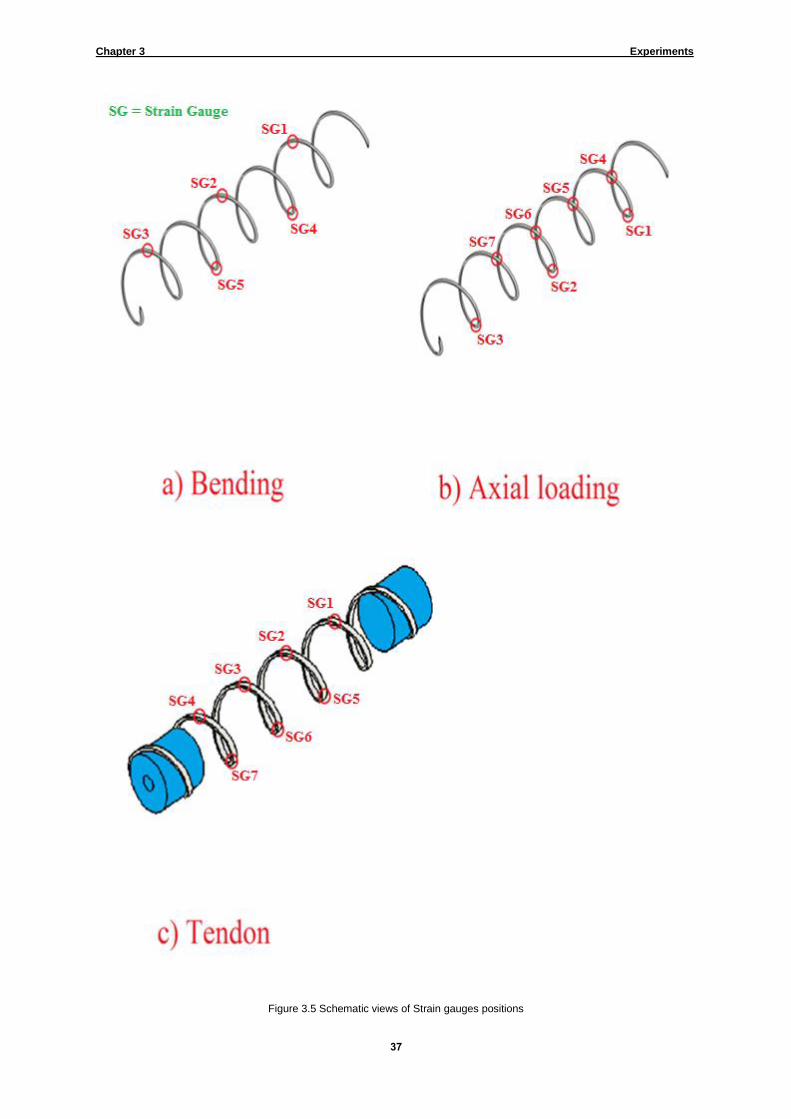
Chapter 3 Experiments
37
Figure 3.5 Schematic views of Strain gauges positions

Chapter 3 Experiments
38
3.4 Scorpio
Scorpio is a computer program that reads and plots the information of strain gauges. The
Scorpio software includes five applications shown in figure 3.6. They are:
Figure 3.6 Scorpio applications and their icons (Solartron Instruments Ltd., 1993)
a) Scorpio System Configuration: It was shown by the first icon on the left in figure 3.6.
The main application that prepares the PC system for starting the other four applications.
b) Measurement Setup: Using three methods, this application is responsible for preparing
the data logger for measuring data; the methods are:
File: the logger commands are sent through a disk-based file; this file can be
prepared via either Learn feature or editing text feature.
Interactive: in the data logger a command line is saved for further control or plotting.
Panel: data logger front panel is simulated.
c) Monitor: This application for displaying raw data from connected logger(s). The data is
divided to three types:
Channels: They are separated measurements of the tasks.
Task: A single test results taken from the data logger are assembled in the task.
Headers: Are the “Task-headers” gathered from all tasks of the data logger and
plotted on the screen.
Measurement setup application controls the Monitor results through its local on/off
options.

Chapter 3 Experiments
39
d) Live Results: It is used to show, plot, save and export the live results data when it was
necessary; the data might be demonstrated as:
Text, for the task.
Trend graphs, for the channels.
Transient data through two options might be saved:
Interactive: The data is plotted in a chart and components can be saved in the disk.
Standalone: The data is taken continuously and saved directly to the disk but no plot
is provided.
e) Historical Results: The already saved-to-disk data can be record and playback with this
application through either the PC or the data logger. From this application data can be
transferred to Microsoft Excel, which is more reliable.
3.5 INSTRON 8801 Loading Machine
INSTRON 8801 is a loading machine designed for fatigue testing systems. The maximum
load capacity of the machine is 100kN, which is bigger than the maximum loads required for
the experiments. It is possible to apply any static or dynamic tests via this instrument
including high/low cyclic loading, thermal fatigue experiments and mechanics of fracture. A
picture of this instrument is shown in figure 3.7 (Illinois Tool Works Inc., 2012).
The machine has an operator panel facility which proves users immediate feedback on
setting of any test (figure 3.8). So, it is possible to instantly check the operating modes;
position, real time load, number of cycles, strain status, wearing, errors. No PC is required
when panel is available. (Illinois Tool Works Inc., 2008).

Chapter 3 Experiments
41
Figure 3.7 INSTRON 8801 (Illinois Tool Works Inc., 2012)
Figure 3.8 Series 8800 Operating Panel (Illinois Tool Works Inc., 2008)

Chapter 3 Experiments
40
3.6 Tests on Helical Tendon
3.6.1 Tensile Dead Loading
One of the major concerns in flexible risers is fatigue failures observed in helical wires. The
aim of this test is to measure the effects of static loads on the deformation and strain
changes of single helical tendon layer before the reliability of tendon reached the creep-
curved conditions.
In figure 3.9, a single tendon specimen with two metallic cylinders at both ends is shown.
The process of loading is called dead loading, in which the specimen is tested under static
tensile loads; using a hanger, various weights are added to apply a specific value of load on
the specimen. A hanger with the mass of 1.75 kg was used. The initial length of the
specimen without hangers was 630mm; the length with the hanger was 715mm, which was
assumed as initial length in the analysis. The maximum possible value for loading was 2kg.
It is shown in figures 3.10 and 3.11 how the test components assembled, placed and tested.
The results of dead loading experiments were used to validate the accuracy of the numerical
models in the next chapter. Here, only two samples (one for displacement and one for strain
changes) of these results have shown in figures 3.12 and 3.13.
Figure 3.9 Tendon with two cylinders

Chapter 3 Experiments
42
Figure 3.10 Hanger components
Figure 3.11 Tendon - Testing
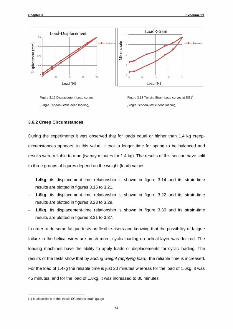
Chapter 3 Experiments
43
Figure 3.12 Displacement-Load curves Figure 3.13 Tensile Strain-Load curves at SG11
[Single Tendon-Static dead loading] [Single Tendon-Static dead loading]
3.6.2 Creep Circumstances
During the experiments it was observed that for loads equal or higher than 1.4 kg creep-
circumstances appears; in this value, it took a longer time for spring to be balanced and
results were reliable to read (twenty minutes for 1.4 kg). The results of this section have split
to three groups of figures depend on the weight (load) values:
1.4kg, its displacement-time relationship is shown in figure 3.14 and its strain-time
results are plotted in figures 3.15 to 3.21,
1.6kg, its displacement-time relationship is shown in figure 3.22 and its strain-time
results are plotted in figures 3.23 to 3.29,
1.8kg, its displacement-time relationship is shown in figure 3.30 and its strain-time
results are plotted in figures 3.31 to 3.37.
In order to do some fatigue tests on flexible risers and knowing that the possibility of fatigue
failure in the helical wires are much more, cyclic loading on helical layer was desired. The
loading machines have the ability to apply loads or displacements for cyclic loading. The
results of the tests show that by adding weight (applying load), the reliable time is increased.
For the load of 1.4kg the reliable time is just 20 minutes whereas for the load of 1.6kg, it was
45 minutes, and for the load of 1.8kg, it was increased to 80 minutes.
(1) In all sections of this thesis SG means strain gauge
0
1.875
3.75
5.625
7.5
17 20 23 26 29
Dis
pla
cem
ent
(mm
)
Load (N)
Load-Displacement
Experiment
-1
1
3
5
7
17 20 23 26 29
Mic
ro s
trai
n
Load (N)
Load-Strain
Experiment

Chapter 3 Experiments
44
Figure 3.14 Displacement-Time curve Figure 3.15 Strain-Time curve at SG 1
[Single Tendon-Creep Curve-1.4 kg] [Single Tendon-Creep Curve-1.4 kg]
Figure 3.16 Strain-Time curve at SG 2 Figure 3.17 Strain-Time curve at SG 3
[Single Tendon-Creep Curve-1.4 kg] [Single Tendon-Creep Curve-1.4 kg]
Figure 3.18 Strain-Time curve at SG 4 Figure 3.19 Strain-Time curve at SG 5
[Single Tendon-Creep Curve-1.4 kg] [Single Tendon-Creep Curve-1.4 kg]
8.9
9.1
9.3
9.5
0 5 10 15 20
Dis
pla
cem
ent
(mm
)
Time (min)
Displacement - Time
-70
-40
-10
20
0 5 10 15 20
Mic
ro s
trai
n
Time (min)
Strain - Time
Torsion
Tensile
-40
-30
-20
-10
0 5 10 15 20
Mic
ro s
trai
n
Time (min)
Strain - Time
Torsion
Tensile
-40
-30
-20
-10
0 5 10 15 20
Mic
ro s
trai
n
Time (min)
Strain - Time
Torsion
Tensile
-40
-30
-20
-10
0
0 5 10 15 20
Mic
ro s
trai
n
Time (min)
Strain - Time
TorsionTensile
-64
-46.5
-29
-11.5
6
0 5 10 15 20
Mic
ro s
trai
n
Time (min)
Strain - Time
TorsionTensile

Chapter 3 Experiments
45
Figure 3.20 Strain-Time curve at SG 6 Figure 3.21 Strain-Time curve at SG 7
[Single Tendon-Creep Curve-1.4 kg] [Single Tendon-Creep Curve-1.4 kg]
Figure 3.22 Displacement-Time curve Figure 3.23 Strain-Time curve at SG 1
[Single Tendon-Creep Curve-1.6 kg] [Single Tendon-Creep Curve-1.6 kg]
Figure 3.24 Strain-Time curve at SG 2 Figure 3.25 Strain-Time curve at SG 3
[Single Tendon-Creep Curve-1.6 kg] [Single Tendon-Creep Curve-1.6 kg]
-31
-29.75
-28.5
-27.25
-26
0 5 10 15 20
Mic
ro s
trai
n
Time (min)
Strain - Time
Torsion
Tensile
-65
-50
-35
-20
-5
0 5 10 15 20
Mic
ro s
trai
n
Time (min)
Strain - Time
Torsion
Tensile
11
11.5
12
12.5
0 15 30 45
Dis
pla
cem
ent
(mm
)
Time (min)
Displacement - Time
-95
-60
-25
10
45
0 15 30 45
Mic
ro s
trai
n
Time (min)
Strain - Time
Torsion
Tensile
-45
-35
-25
-15
-5
0 15 30 45
Mic
ro s
trai
n
Time (min)
Strain - Time
Torsion
Tensile
-50
-40
-30
-20
-10
0 15 30 45
Mic
ro s
trai
n
Time (min)
Strain - Time
Torsion
Tensile

Chapter 3 Experiments
46
Figure 3.26 Strain-Time curve at SG 4 Figure 3.27 Strain-Time curve at SG 5
[Single Tendon-Creep Curve-1.6 kg] [Single Tendon-Creep Curve-1.6 kg]
Figure 3.28 Strain-Time curve at SG 6 Figure 3.29 Strain-Time curve at SG 7
[Single Tendon-Creep Curve-1.6 kg] [Single Tendon-Creep Curve-1.6 kg]
Figure 3.30 Displacement-Time curve Figure 3.31 Strain-Time curve at SG 1
[Single Tendon-Creep Curve-1.8 kg] [Single Tendon-Creep Curve-1.8 kg]
-50
-35
-20
-5
10
0 15 30 45
Mic
ro s
trai
n
Time (min)
Strain - Time
Torsion
Tensile
-85
-57.5
-30
-2.5
25
0 15 30 45
Mic
ro s
trai
n
Time (min)
Strain - Time
Torsion
Tensile
-35.5
-33.875
-32.25
-30.625
-29
0 15 30 45
Mic
ro s
trai
n
Time (min)
Strain - Time
Torsion
Tensile
-71
-53.5
-36
-18.5
-1
0 15 30 45
Mic
ro s
trai
n
Time (min)
Strain - Time
Torsion
Tensile
13.5
14.625
15.75
16.875
18
0 20 40 60 80
Dis
pla
cem
ent
(mm
)
Time (min)
Displacement - Time
-130
-80
-30
20
70
0 20 40 60 80
Mic
ro s
trai
n
Time (min)
Strain - Time
TorsionTensile

Chapter 3 Experiments
47
Figure 3.32 Strain-Time curve at SG 2 Figure 3.33 Strain-Time curve at SG 3
[Single Tendon-Creep Curve-1.8 kg] [Single Tendon-Creep Curve-1.8 kg]
Figure 3.34 Strain-Time curve at SG 4 Figure 3.35 Strain-Time curve at SG 5
[Single Tendon-Creep Curve-1.8 kg] [Single Tendon-Creep Curve-1.8 kg]
Figure 3.36 Strain-Time curve at SG 6 Figure 3.37 Strain-Time curve at SG 7
[Single Tendon-Creep Curve-1.8 kg] [Single Tendon-Creep Curve-1.8 kg]
-53
-42.25
-31.5
-20.75
-10
0 20 40 60 80
Mic
ro s
trai
n
Time (min)
Strain - Time
TorsionTensile
-80
-62.5
-45
-27.5
-10
0 20 40 60 80
Mic
ro s
trai
n
Time (min)
Strain - Time
TorsionTensile
-50
-35
-20
-5
10
0 20 40 60 80
Mic
ro s
trai
n
Time (min)
Strain - Time
Torsion
Tensile
-140
-95
-50
-5
40
0 20 40 60 80
Mic
ro s
trai
n
Time (min)
Strain - Time
Torsion
Tensile
-54
-49
-44
-39
-34
0 20 40 60 80
Mic
ro s
trai
n
Time (min)
Strain - Time
Torsion
Tensile
-100
-75
-50
-25
0
0 20 40 60 80
Mic
ro s
trai
n
Time (min)
Strain - Time
Torsion
Tensile
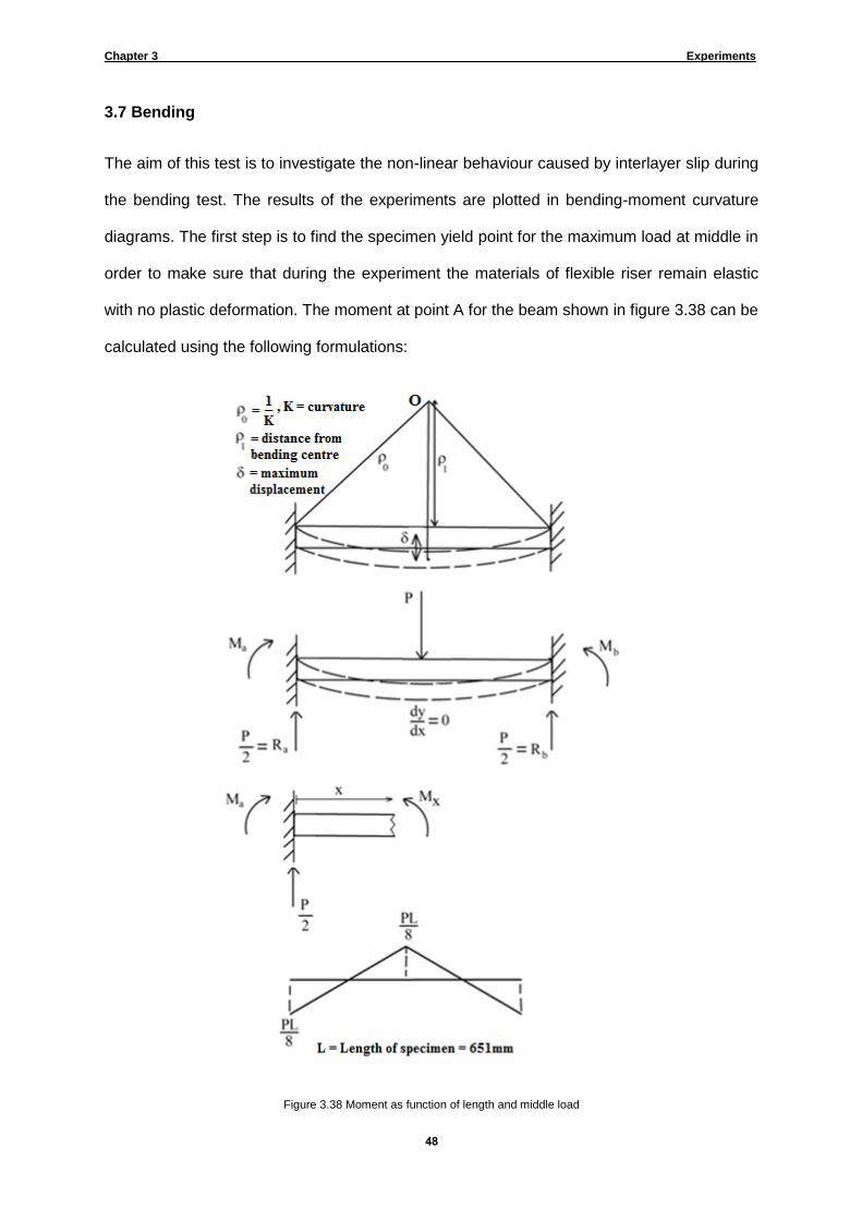
Chapter 3 Experiments
48
3.7 Bending
The aim of this test is to investigate the non-linear behaviour caused by interlayer slip during
the bending test. The results of the experiments are plotted in bending-moment curvature
diagrams. The first step is to find the specimen yield point for the maximum load at middle in
order to make sure that during the experiment the materials of flexible riser remain elastic
with no plastic deformation. The moment at point A for the beam shown in figure 3.38 can be
calculated using the following formulations:
Figure 3.38 Moment as function of length and middle load

Chapter 3 Experiments
49
(3.2)
For bending, we know that
, (3.3)
Where is bending moment, is the distance between bending neutral axis and bended
surfaces = inner radius of inner tube: ,
is area moment inertia, calculated from:
[
]
[ ] .
Knowing that yield stress is 60MPa from CES1 selector software, yield moment and load are:
In order to study the inter-layer non-linear effects without reaching yield point, the maximum
load used for bending test was 13kN, which was lower than 16.88kN. The value of curvature
for bending can be calculated from:
[
]
(3.4)
In order to use equation 3.4 for measuring curvature at each load increment, nine
displacement transducers were placed under the specimen. However, the displacements of
two points at the end of each side were ignored because of the negligible small values. So
(1) Cambridge material selector software

Chapter 3 Experiments
51
effectively, seven displacement transducers were used for the analysis. The space between
the displacement transducer was 65.1 mm (figure 3.39).
The accuracy of displacement measurement is one hundredth of millimetre. On direction of
helical tendon, five strain gauges were installed with the accuracy of a micro-strain (figure
3.40). The bending load is increased and decreased in 105 steps with the load increment of
250N (figure 3.41).
Each displacement transducer was installed on a variable sized metallic base. The
maximum load value could not exceed 13kN in practice. This was because at this load the
lowest part of outer tube touched the top surface of one base; thus, more loading was
practically impossible.
For controlling oil and letting the air to exit easily while pressure oil is induced inside the
inner-tube, two valves were designed which are shown in figure 3.42. The air notch had to
be drilled in higher position to evacuate more air at the same time as oil was pressured in
(left side of figure 3.42). As demonstrated in the right side of the figure 3.42, in oder to
observe and control the oil pressure, a pressure gauge and a valve (black) placed
respectively between the end-cap and one-way oil valve. A one way valve designed to
dispatch oil-pump easily. Bed is positioned on INSTRON loading machine with three M20
bolts in middle.

Chapter 3 Experiments
50
Figure 3.39 Specimen for bending test: displacement transducers positions
Figure 3.40 Strain gauge of the helical tendon

Chapter 3 Experiments
52
Figure 3.41 Schematic view of load increments versus time
Figure 3.42 Specimen for bending test: air valve on the left, and oil components on the right
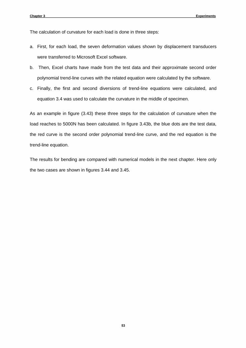
Chapter 3 Experiments
53
The calculation of curvature for each load is done in three steps:
a. First, for each load, the seven deformation values shown by displacement transducers
were transferred to Microsoft Excel software.
b. Then, Excel charts have made from the test data and their approximate second order
polynomial trend-line curves with the related equation were calculated by the software.
c. Finally, the first and second diversions of trend-line equations were calculated, and
equation 3.4 was used to calculate the curvature in the middle of specimen.
As an example in figure (3.43) these three steps for the calculation of curvature when the
load reaches to 5000N has been calculated. In figure 3.43b, the blue dots are the test data,
the red curve is the second order polynomial trend-line curve, and the red equation is the
trend-line equation.
The results for bending are compared with numerical models in the next chapter. Here only
the two cases are shown in figures 3.44 and 3.45.

Chapter 3 Experiments
54
a)
b)
Trend line equation
K (
)
0.0399998
c)
Figure 3.43 a) step1: Deformation measurements, b) step2: Resulted chart, c) Final calculation of curvature
(1) maximum value of x = xmax = L = 651mm
y = 2E-05x2 - 0.0158x - 59.985
-63
-61.5
-60
0 220 440 660
y
x (xmax = L = 651)
Load (N) x1 y + dy
5000
0 -60
130.2 -61.57
195.3 -62.18
260.4 -62.44
325.5 -62.57
390.6 -62.45
455.7 -62.19
520.8 -61.55
651 -60
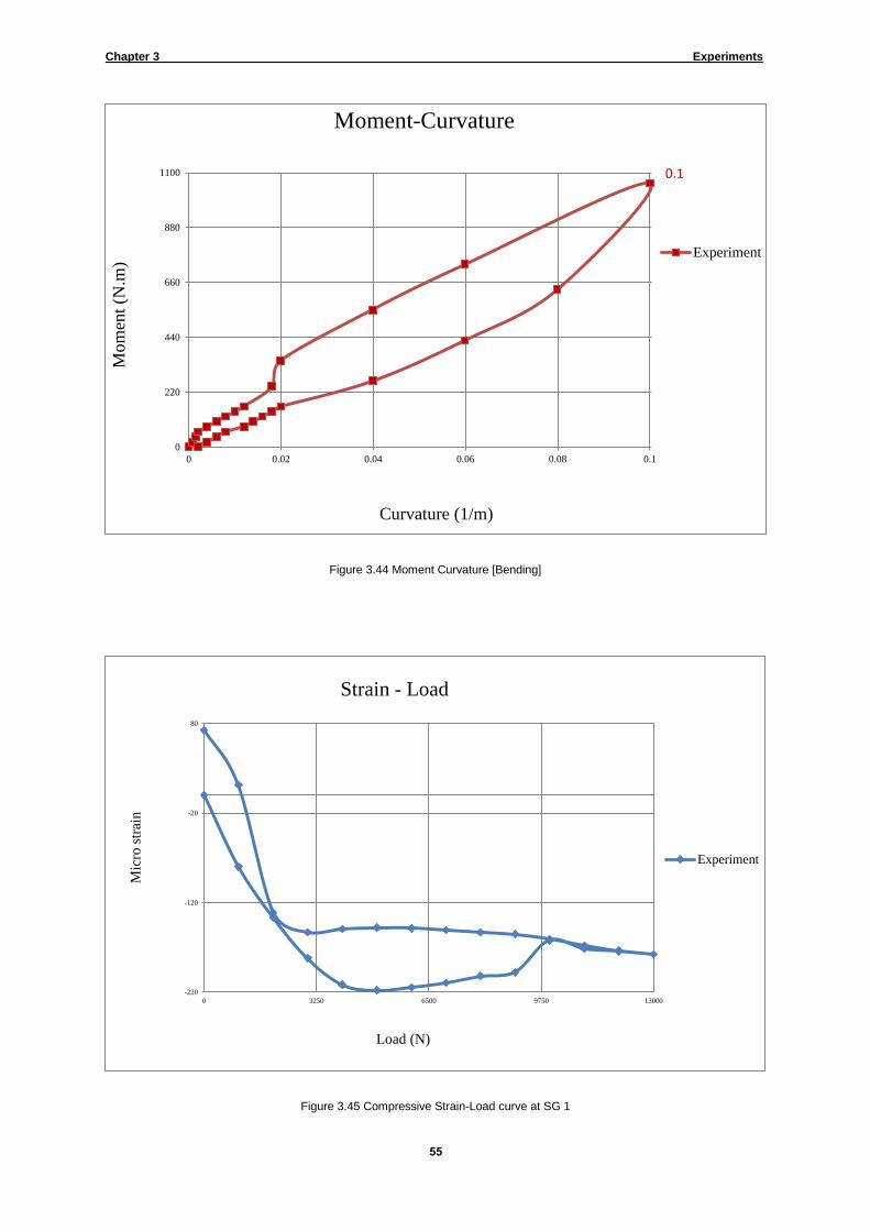
Chapter 3 Experiments
55
Figure 3.44 Moment Curvature [Bending]
Figure 3.45 Compressive Strain-Load curve at SG 1
0.1
0
220
440
660
880
1100
0 0.02 0.04 0.06 0.08 0.1
Mom
ent
(N.m
)
Curvature (1/m)
Moment-Curvature
Experiment
-220
-120
-20
80
0 3250 6500 9750 13000
Mic
ro s
trai
n
Load (N)
Strain - Load
Experiment

Chapter 3 Experiments
56
3.8 Axial Loading (Compressive)
Many axial loading tests were performed in this study under various conditions shown in
tables 3.1 and 3.2. Although there are sixteen different tests, only the results of a few tests
are presented in this chapter. The rest are shown in appendix A.
Table 3.3 List of Axial tests (Air Pressure)1
Test No. Layer(s) with strain-gauges Maximum Load (kN) Pressure (bar)
01 Inner tube 15 1
02 3 1
03 Outer Tube and Helical Tendon 15 1
04 3 1
Table 3.4 List of Axial tests (Oil Pressure)
Test No. Layer(s) with strain-gauges Maximum Load (kN) Pressure (bar)
05
Inner tube
3
1
06 5
07 10
08 15
09 20
10 No load 1,5,10,12,14,16,18,20
11
Outer Tube and Helical Tendon
3
1
12 5
13 10
14 15
15 20
16 No load 1,5,10,12,14,16,18,20
A large number of wires were attached to strain gauges related to these layers and it was
not possible to attach the wires to both strain gauges on the inner and outer tube at the
same time. So the tests for every load and pressure were performed twice; first inner tube
was measured and then outer tube and helical tendon was studied. To prevent inducing
unwanted moment from non axi-symmetric design of bending end-caps, the end-caps design
(1) For all axial tests the increment for 15000N was 500N and for 3000N it was 200N.

Chapter 3 Experiments
57
become curved for axial tests, which were lighter as well. The prototype assembly for axial
loading is shown in figure 3.46. An L shape notch at the bottom and a notch at the top were
drilled for oil injecting and air eviction respectively; all oil components of previous tests were
used beneath the specimen (figure 3.47). Leakage has been checked before starting the
test; the maximum available value of oil pressure, which is twenty bars, was applied
continuously for a while. This was a check to make sure that there is no risk to the safety of
the people and the loading machine during the experiment (figures 3.46 to 3.48).
Two displacement transducers were used: one for vertical deformation and the other for the
buckling changes (figure 3.49). Seven strain gauges were installed on the crucial layers,
which are inner-tube, tendon, and outer tube. To measure the strain changes two types of
strain gauges one suitable for polymers and one for metal were used (figure 3.50).
Figure 3.46 Leakage checking at maximum pressure 1 - assembly view

Chapter 3 Experiments
58
Figure 3.47 Leakage checking at maximum pressure 2 - Pressure gauge at 20bar (maximum)
Figure 3.48 Leakage checking at maximum pressure 3 – Releasing oil

Chapter 3 Experiments
59
Figure 3.49 Compressive testing for inner tube
Figure 3.50 Strain gauge for metal tendon (Right) and polymer Tubes (Left)

Chapter 3 Experiments
61
3.8.1 Pressure Effects with No External Load
The aim of this study was to demonstrate the pure effect of pressure on the deformation and
strain changes. The displacement-load relationship has been plotted in figure 3.51. The
displacement-load figure shows that there was a strong non-linear behaviour at deformation
trend in particular between 10 to 20 bar. During unloading, the residual stresses kept the
deformed specimen in similar situation until the value has decreased to the half of maximum
pressure, ten bar; at this point the trend had a similar pattern to the previous process. Finally
in the end there are residual stresses at specimen. The figure demonstrates that even small
internal pressure value, may activate the interlayer behaviour of flexible pipe.
In figures 3.52 to 3.65 the strain changes versus pressure are demonstrated. In two cases
figure 3.52 and 3.58 due to a problem in the strain gauges it was not possible to measure
strains. For helical tendon, the induced torsion results had less residual strains comparing to
compression; this means, the pressure had less effects on helix at torsion direction
comparing to compressive direction. Except gauge number seven, the trend of compression
indicate residual strains at the end. For torsion trends, except gauge number six, there are
residual strains. The torsion trends are not similar in terms of direction as each gauge local
position is different. For outer tube, similar to previous part, the compressive residual strains
were larger than the results of buckling. The figures have shown that the trends are similar
for buckling and compression.
Figure 3.51 Displacement-Pressure curves [Axial-Outer Tube and Helical Tendon-pure pressure effects]
0
0.055
0.11
0.165
0.22
0 5 10 15 20
Dis
pla
cem
ent
(mm
)
Pressure (bar)
Displacement - Pressure
Loading
Unloading
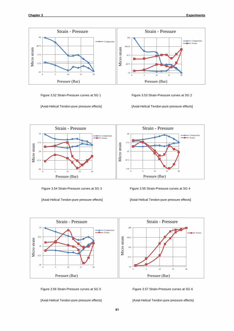
Chapter 3 Experiments
60
Figure 3.52 Strain-Pressure curves at SG 1 Figure 3.53 Strain-Pressure curves at SG 2
[Axial-Helical Tendon-pure pressure effects] [Axial-Helical Tendon-pure pressure effects]
Figure 3.54 Strain-Pressure curves at SG 3 Figure 3.55 Strain-Pressure curves at SG 4
[Axial-Helical Tendon-pure pressure effects] [Axial-Helical Tendon-pure pressure effects]
Figure 3.56 Strain-Pressure curves at SG 5 Figure 3.57 Strain-Pressure curves at SG 6
[Axial-Helical Tendon-pure pressure effects] [Axial-Helical Tendon-pure pressure effects]
-25
-3.75
17.5
38.75
60
0 5 10 15 20
Mic
ro s
trai
n
Pressure (Bar)
Strain - Pressure
Compression
-10
28.75
67.5
106.25
145
0 5 10 15 20
Mic
ro s
trai
n
Pressure (Bar)
Strain - Pressure
Compression
Tosion
-95
-57.5
-20
17.5
55
0 5 10 15 20
Mic
ro s
trai
n
Pressure (Bar)
Strain - Pressure
Compression
Tosion
-110
-67.5
-25
17.5
60
0 5 10 15 20
Mic
ro s
trai
n
Pressure (Bar)
Strain - Pressure
Compression
Tosion
-35
-12.5
10
32.5
55
0 5 10 15 20
Mic
ro s
trai
n
Pressure (Bar)
Strain - Pressure
Compression
Tosion
-10
57.5
125
192.5
260
0 5 10 15 20
Mic
ro s
trai
n
Pressure (Bar)
Strain - Pressure
Tosion

Chapter 3 Experiments
62
Figure 3.58 Strain-Pressure curves at SG 7 Figure 3.59 Strain-Pressure curves at SG 1
[Axial-Helical Tendon-pure pressure effects] [Axial-Outer Tube-pure pressure effects]
Figure 3.60 Strain-Pressure curves at SG 2 Figure 3.61 Strain-Pressure curves at SG 3
[Axial-Outer Tube-pure pressure effects] [Axial-Outer Tube-pure pressure effects]
Figure 3.62 Strain-Pressure curves at SG 4 Figure 3.63 Strain-Pressure curves at SG 5
[Axial-Outer Tube-pure pressure effects] [Axial-Outer Tube-pure pressure effects]
-105
-77.5
-50
-22.5
5
0 5 10 15 20
Mic
ro s
trai
n
Pressure (Bar)
Strain - Pressure
Compression
-160
-42.5
75
192.5
310
0 5 10 15 20
Mic
ro s
trai
n
Pressure (Bar)
Strain - Pressure
Compression
Buckling
-50
22.5
95
167.5
240
0 5 10 15 20
Mic
ro s
trai
n
Pressure (Bar)
Strain - Pressure
CompressionBuckling
-50
15
80
145
210
0 5 10 15 20
Mic
ro s
trai
n
Pressure (Bar)
Strain - Pressure
CompressionBuckling
-120
-35
50
135
220
0 5 10 15 20
Mic
ro s
trai
n
Pressure (Bar)
Strain - Pressure
CompressionBuckling
-100
-22.5
55
132.5
210
0 5 10 15 20
Mic
ro s
trai
n
Pressure (Bar)
Strain - Pressure
CompressionBuckling
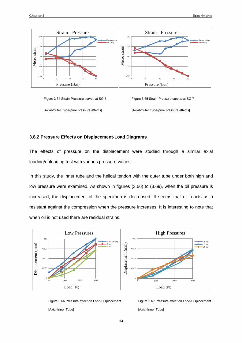
Chapter 3 Experiments
63
Figure 3.64 Strain-Pressure curves at SG 6 Figure 3.65 Strain-Pressure curves at SG 7
[Axial-Outer Tube-pure pressure effects] [Axial-Outer Tube-pure pressure effects]
3.8.2 Pressure Effects on Displacement-Load Diagrams
The effects of pressure on the displacement were studied through a similar axial
loading/unloading test with various pressure values.
In this study, the inner tube and the helical tendon with the outer tube under both high and
low pressure were examined. As shown in figures (3.66) to (3.69), when the oil pressure is
increased, the displacement of the specimen is decreased. It seems that oil reacts as a
resistant against the compression when the pressure increases. It is interesting to note that
when oil is not used there are residual strains.
Figure 3.66 Pressure effect on Load-Displacement Figure 3.67 Pressure effect on Load-Displacement
[Axial-Inner Tube] [Axial-Inner Tube]
-190
-80
30
140
250
0 5 10 15 20
Mic
ro s
trai
n
Pressure (Bar)
Strain - Pressure
CompressionBuckling
-300
-172.5
-45
82.5
210
0 5 10 15 20
Mic
ro s
trai
n
Pressure (Bar)
Strain - Pressure
CompressionBuckling
0
0.0175
0.035
0.0525
0.07
0 1000 2000 3000
Dis
pla
cem
ent
(mm
)
Load (N)
Low Pressures
1 bar (no oil)
1 bar
5 bar
0
0.0175
0.035
0.0525
0.07
0 1000 2000 3000
Dis
pla
cem
ent
(mm
)
Load (N)
High Pressures
10 bar
15 bar
20 bar
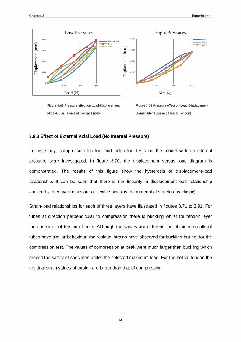
Chapter 3 Experiments
64
Figure 3.68 Pressure effect on Load-Displacement Figure 3.69 Pressure effect on Load-Displacement
[Axial-Outer Tube and Helical Tendon] [Axial-Outer Tube and Helical Tendon]
3.8.3 Effect of External Axial Load (No Internal Pressure)
In this study, compression loading and unloading tests on the model with no internal
pressure were investigated. In figure 3.70, the displacement versus load diagram is
demonstrated. The results of this figure show the hysteresis of displacement-load
relationship. It can be seen that there is non-linearity in displacement-load relationship
caused by interlayer behaviour of flexible pipe (as the material of structure is elastic).
Strain-load relationships for each of three layers have illustrated in figures 3.71 to 3.91. For
tubes at direction perpendicular to compression there is buckling whilst for tendon layer
there is signs of torsion of helix. Although the values are different, the obtained results of
tubes have similar behaviour; the residual strains have observed for buckling but not for the
compression test. The values of compression at peak were much larger than buckling which
proved the safety of specimen under the selected maximum load. For the helical tendon the
residual strain values of torsion are larger than that of compression.
0
0.018
0.036
0.054
0.072
0 1000 2000 3000
Dis
pla
cem
ent
(mm
)
Load (N)
Low Pressures
1 bar (no oil)
1 bar
5 bar
0
0.018
0.036
0.054
0.072
0 1000 2000 3000
Dis
pla
cem
ent
(mm
)
Load (N)
Hight Pressures
10 bar
15 bar
20 bar

Chapter 3 Experiments
65
Figure 3.70 Displacement-Load curve [Axial-no-oil-15kN max]
Figure 3.71 Strain-Load curve at SG 1 Figure 3.72 Strain-Load curve at SG 2
[Axial-Inner Tube-no oil-15kN max] [Axial-Inner Tube-no oil-15kN max]
Figure 3.73 Strain-Load curve at SG 3 Figure 3.74 Strain-Load curve at SG 4
[Axial-Inner Tube-no oil-15kN max] [Axial-Inner Tube-no oil-15kN max]
0
0.1
0.2
0.3
0.4
0.5
0.6
0.7
0 3000 6000 9000 12000 15000D
isp
lace
men
t (m
m)
Load (N)
Displacement - Load
-550
-400
-250
-100
50
200
0 3000 6000 9000 12000 15000
Mic
ro s
trai
n
Load (N)
Strain - Load
Buckling
Compression
-650
-400
-150
100
350
0 3000 6000 9000 12000 15000
Mic
ro s
trai
n
Load (N)
Strain - Load
Buckling
Compression
-660
-456
-252
-48
156
360
0 3000 6000 9000 12000 15000
Mic
ro s
trai
n
Load (N)
Strain - Load
Buckling
Compression
-710
-504
-298
-92
114
320
0 3000 6000 9000 12000 15000
Mic
ro s
trai
n
Load (N)
Strain - Load
Buckling
Compression

Chapter 3 Experiments
66
Figure 3.75 Strain-Load curve at SG 5 Figure 3.76 Strain-Load curve at SG 6
[Axial-Inner Tube-no oil-15kN max] [Axial-Inner Tube-no oil-15kN max]
Figure 3.77 Strain-Load curve at SG 7 Figure 3.78 Strain-Load curve at SG 1
[Axial-Inner Tube-no oil-15kN max] [Axial-Helical Tendon-no oil-15kN max]
Figure 3.79 Strain-Load curve at SG 2 Figure 3.80 Strain-Load curve at SG 3
[Axial-Helical Tendon-no oil-15kN max] [Axial-Helical Tendon-no oil-15kN max]
-710
-524
-338
-152
34
220
0 3000 6000 9000 12000 15000
Mic
ro s
trai
n
Load (N)
Strain - Load
Buckling
Compression
-650
-460
-270
-80
110
300
0 3000 6000 9000 12000 15000
Mic
ro s
trai
n
Load (N)
Strain - Load
Buckling
Compression
-670
-464
-258
-52
154
360
0 3000 6000 9000 12000 15000
Mic
ro s
trai
n
Load (N)
Strain - Load
Buckling
Compression
0
3.5
7
10.5
14
0 3000 6000 9000 12000 15000
Mic
ro s
trai
n
Load (N)
Strain - Load
TorsionCompression
-2
2.5
7
11.5
16
0 3000 6000 9000 12000 15000
Mic
ro s
trai
n
Load (N)
Strain - Load
TorsionCompression
-2
3
8
13
18
0 3000 6000 9000 12000 15000
Mic
ro s
trai
n
Load (N)
Strain - Load
TorsionCompression

Chapter 3 Experiments
67
Figure 3.81 Strain-Load curve at SG 4 Figure 3.82 Strain-Load curve at SG 5
[Axial-Helical Tendon-no oil-15kN max] [Axial-Helical Tendon-no oil-15kN max]
Figure 3.83 Strain-Load curve at SG 6 Figure 3.84 Strain-Load curve at SG 7
[Axial-Helical Tendon-no oil-15kN max] [Axial-Helical Tendon-no oil-15kN max]
Figure 3.85 Strain-Load curve at SG 1 Figure 3.86 strain-Load curve at SG 2
[Axial-Outer Tube-no oil-15kN max] [Axial-Outer Tube-no oil-15kN max]
Figure 5.87 Strain-Load curve at SG 3 Figure 5.88 Strain-Load curve at SG 4
[Axial-Outer Tube-no oil-15kN max] [Axial-Outer Tube-no oil-15kN max]
-1
2
5
8
11
0 3000 6000 9000 12000 15000
Mic
ro s
trai
n
Load (N)
Strain - Load Torsion
Compression
-1
4.25
9.5
14.75
20
0 3000 6000 9000 12000 15000
Mic
ro s
trai
n
Load (N)
Strain - Load
Torsion
Compression
-1
2.25
5.5
8.75
12
0 3000 6000 9000 12000 15000
Mic
ro s
trai
n
Load (N)
Strain - Load Torsion
-2
2.25
6.5
10.75
15
0 3000 6000 9000 12000 15000
Mic
ro s
trai
n
Load (N)
Strain - Load TorsionCompression
-350
-250
-150
-50
50
150
0 3000 6000 9000 12000 15000
Mic
ro s
trai
n
Load (N)
Strain - Load Buckling
Compression
-400
-247.5
-95
57.5
210
0 3000 6000 9000 12000 15000
Mic
ro s
trai
n
Load (N)
Strain - Load Buckling
Compression
-470
-292.5
-115
62.5
240
0 3000 6000 9000 12000 15000
Mic
ro s
trai
n
Load (N)
Strain - Load Buckling
Compression
-540
-340
-140
60
260
0 3000 6000 9000 12000 15000
Mic
ro s
trai
n
Load (N)
Strain - Load
Buckling
Compression

Chapter 3 Experiments
68
Figure 5.89 Strain-Load curve at SG 5 Figure 5.90 Strain-Load curve at SG 6
[Axial-Outer Tube-no oil-15kN max] [Axial-Outer Tube-no oil-15kN max]
Figure 5.91 Strain-Load curve at SG 7
[Axial-Outer Tube-no oil-15kN max]
3.9 Conclusion
Several experiments on a prototype of flexible pipe were conducted to investigate its non-
linear behaviour caused by interlayer slip during bending and axial loading tests. The effect
of static loads on the deformation and strain changes of a single helical tendon layer was
also investigated. A strong non-linear behaviour in both the bending and the axial load tests
were observed. The experimental results can be used as a benchmark solution to
investigate the accuracy of various FE based models for analysing flexible pipes.
-590
-365
-140
85
310
0 3000 6000 9000 12000 15000
Mic
ro s
trai
n
Load (N)
Strain - Load Buckling
Compression
-600
-375
-150
75
300
0 3000 6000 9000 12000 15000
Mic
ro s
trai
n
Load (N)
Strain - Load Buckling
Compression
-550
-340
-130
80
290
0 3000 6000 9000 12000 15000
Mic
ro s
trai
n
Load (N)
Strain - Load Buckling
Compression

Chapter 4:
Numerical Modelling
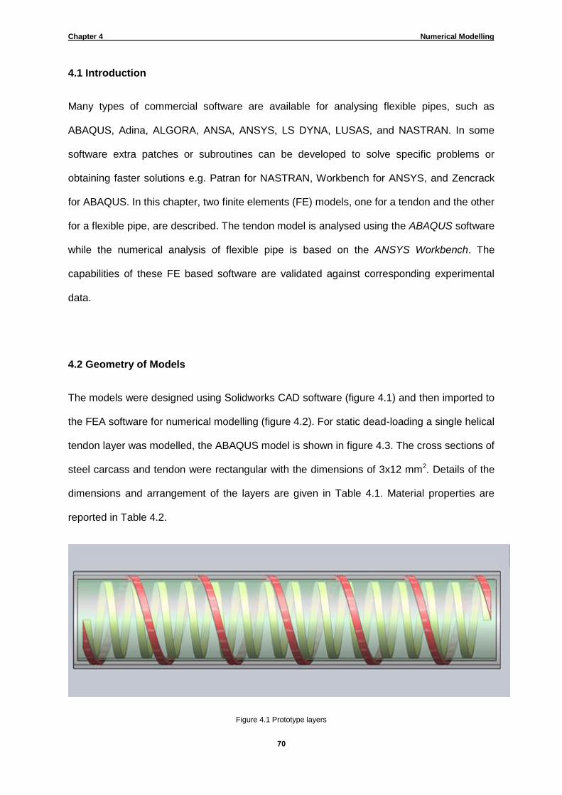
Chapter 4 Numerical Modelling
71
4.1 Introduction
Many types of commercial software are available for analysing flexible pipes, such as
ABAQUS, Adina, ALGORA, ANSA, ANSYS, LS DYNA, LUSAS, and NASTRAN. In some
software extra patches or subroutines can be developed to solve specific problems or
obtaining faster solutions e.g. Patran for NASTRAN, Workbench for ANSYS, and Zencrack
for ABAQUS. In this chapter, two finite elements (FE) models, one for a tendon and the other
for a flexible pipe, are described. The tendon model is analysed using the ABAQUS software
while the numerical analysis of flexible pipe is based on the ANSYS Workbench. The
capabilities of these FE based software are validated against corresponding experimental
data.
4.2 Geometry of Models
The models were designed using Solidworks CAD software (figure 4.1) and then imported to
the FEA software for numerical modelling (figure 4.2). For static dead-loading a single helical
tendon layer was modelled, the ABAQUS model is shown in figure 4.3. The cross sections of
steel carcass and tendon were rectangular with the dimensions of 3x12 mm2. Details of the
dimensions and arrangement of the layers are given in Table 4.1. Material properties are
reported in Table 4.2.
Figure 4.1 Prototype layers

Chapter 4 Numerical Modelling
70
Figure 4.2 Workbench model of prototype for Bending
Figure 4.3 Single Tendon model

Chapter 4 Numerical Modelling
72
4.3 Meshing and Element Selection1
Because of geometry, in ANSYS Workbench an eight-node structural element, SOLID185,
for solid load component was used. The element was non-layered type used full integration
and pure displacement (figure 4.4). For riser layers, a four-node shell element SHELL181
with full integration was used. In this element there are two assumptions (figure 4.5):
Normals to the centre-plane after deforming are straight, yet they do not have to remain
perpendicular to centre-plane.
Every Integration points set of any layer in radial direction are similar in terms of element
(or material) orientation.
To keep the load component in a vertical direction for either loading or unloading processes,
there is a need of a frictionless support. So, new surface element SURF154, a three
dimensional structural surface with four nodes (figure 4.6) were used. For Contact, ANSYS
Workbench used two elements CONTA174 and Target170, which are explained in the next
section. In total, 6500 elements were used in the meshing process for the riser model in
ANSYS.
The tendon was assumed solid and an eight node linear brick shaped C3D8R element with
reduced integration and hourglass control was selected in ABAQUS. The node numbering
and the integration point for this element are demonstrated in figure 4.7. Only 150 elements
were required for modelling the tendon in ABAQUS. In figure 4.8, the developed mesh for
the riser in ANSYS Workbench is shown while in figure 4.9 the mesh for tendon layer in
ABAQUS is given.
(1) As demonstrated by ANSYS Inc. (2012) and Dassault Systems (2013).
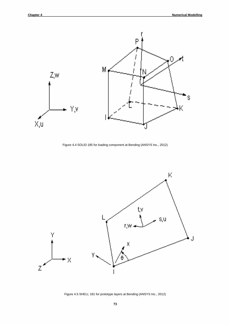
Chapter 4 Numerical Modelling
73
Figure 4.4 SOLID 185 for loading component at Bending (ANSYS Inc., 2012)
Figure 4.5 SHELL 181 for prototype layers at Bending (ANSYS Inc., 2012)

Chapter 4 Numerical Modelling
74
Figure 4.6 SURF 154 [Bending] (ANSYS Inc., 2012)
Figure 4.7: C3D8R Node Numbering and 1x1x1 integration point scheme [Static dead loading] (Dhondt, 2011)
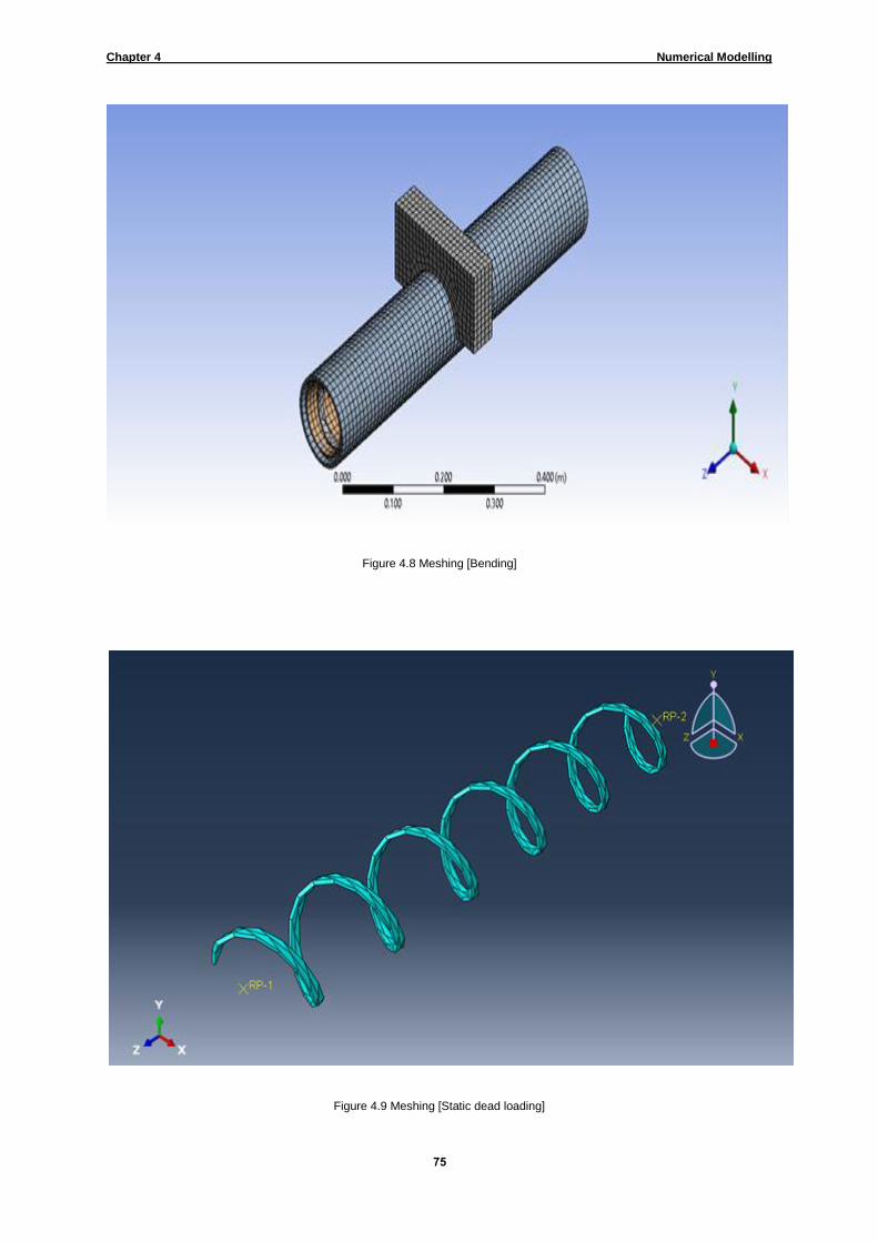
Chapter 4 Numerical Modelling
75
Figure 4.8 Meshing [Bending]
Figure 4.9 Meshing [Static dead loading]

Chapter 4 Numerical Modelling
76
4.4 Contact
There is a three dimensional surface to surface contact between layers and also between
outer tube and loading part. So, a contact modelling technique is required to take into
account the contact effects. Penalty method with Gauss integration points was used to
model contact in ANSYS Workbench. Coefficient of friction between layers is assumed as
0.2. For contact modelling two types of elements have to be defined contact and target.
These elements, defined automatically by ANSYS, are CONTA174 (shown in figure 4.10)
and target 170 in figures 4.11 and 4.12. As shown in figure 4.13, deformable solid materials
are normally defined as contact whereas rigid bodies are defined as targets. In the riser
model, tubes were considered as contact, while helical carcass, helical tendon, and load part
modelled as target. In figure 4.14, contact modelling between outer tube and helical tendon
is demonstrated.
Figure 4.10 CONTA174 [Bending] (ANSYS Inc., 2012)

Chapter 4 Numerical Modelling
77
Figure 4.11 Target170 [Bending] (ANSYS Inc., 2012)
Figure 4.12 Target170 Segment types [Bending] (ANSYS Inc., 2012)

Chapter 4 Numerical Modelling
78
Figure 4.13 Contact detection point at Gauss point [Bending] (ANSYS Inc., 2012)
Figure 4.14 Contact modelling [Bending]

Chapter 4 Numerical Modelling
79
4.5 Load, Boundary Conditions, and Remained Controls
A uniform displacement boundary condition is used to analyse the tendon in ABAQUS. In
this boundary condition all points on the one end section remain in plane throughout the
analysis. An axial force is applied on the other end which gradually increases to 29kN. The
boundary conditions and loading reference points was positioned at centre line of helix at the
both ends (figures 4.15 and 4.16).
Figure 4.15 Schematic view of the Single Helical Tendon study
Figure 4.16 ABAQUS modelled load and boundary conditions using Reference Points [Static dead loading]

Chapter 4 Numerical Modelling
81
For the analysing of the riser in ANSYS, a loading force was applied at the support which is
increased by 250N increment value to reach 13000N (figure 4.17). For unloading test
analysis this value decreased to zero with the same increment. To model this process,
tabular method was used in ANSYS Workbench. To keep load part in its position, a
frictionless support was modelled through four surfaces surrounding the load component
(blue surfaces in figure 4.18). For boundary conditions, one side of the riser modelled as
fixed support whilst the other side can slide freely (see D, E, F, and G signs in figure 4.18).
The numerical modelling of bending was assumed as non-linear problem because the
interlayer effect of pipe structure is non-linear.
Figure 4.17 Schematic view of bending
Figure 4.18 ANSYS modelled load, frictionless support, and boundary conditions [Bending]

Chapter 4 Numerical Modelling
80
4.6 Solution Methods
The solution model used in ANSYS and ABAQUS are briefly explained here (ANSYS Inc.,
2012):
Full Integration, also called method or selective reduced integration, this method
prevents volumetric mesh locking in incompressible models. Volumetric strain at the
Gauss integration point is replaced with the average volumetric strain of elements. The
crucial problem of this way is restrictions in bending problems, where shear locking could
not be ignored. Using the enhanced strain formulation in these conditions is strongly
recommended.
Reduced Integration, similar to previous method, in this method the volumetric mesh
locking in incompressible models is banned. Although this method is much more
accurate in terms of efficiency than full integration method, the accuracy of the respond
is influenced by energy used for hourglass control.
Enhanced Strain Formulation, shear locking for bending and volumetric locking in
incompressible models are prevented in this method. The formulation introduces thirteen
internal DOFs; nine of them are used to overcome shear locking at bending conditions.
In some FE computer programs such as ANSYS these DOFs are made by the software
and are not accessible by the users. Because of extra DOFs, static considerations, and
low efficiency (lower than full integration), this method is roughly selected in the FE
models.
Simplified Enhanced Strain Formulation, similar to previous method, shear locking is
prevented. The number of DOFs is reduced in this method. This means, the number of
DOFs preventing volumetric locking are decreased; thus, the simplified formulation

Chapter 4 Numerical Modelling
82
cannot be used for incompressive materials in most of the models. This method is much
better than previous one because of its lower degrees of freedom, yet full integration
method is better than both of them.
Lagrange Multiplier Method in Contact Elements, in this method, the given internal
energy term is completed through a constraints set which was applied by a Lagrange
multiplier and integrated over its volume, leads to an augmented form. For more details
of this method please refer to appendix C.
For modelling bending in ANSYS, Full Integration method was used. The numerical solution
method used in ABAQUS is Reduced Integration method.

Chapter 4 Numerical Modelling
83
4.7 Results and Discussion
4.7.1 Static Dead Loading
The fatigue failures of tendons in flexible risers are quite common. So, it is important to
examine the predictive ability of FE methods for this layer compared with experimental
results. A schematic model of residual displacements in tendon layer under axial load,
predicted by ABAQUS software, is given in the figure 4.19.
Figure 4.19 Deformation at last second [Static dead loading]
In all results an initial load equivalent to the lighter hanger weight (17.1605N) used in the
experiment is applied. The load is then increased from 17.16N to 29N. The displacement-
load relationship and corresponding experimental data is shown in figure 4.20. The strain-
load results in figures 4.21 to 4.27 are plotted. Both the numerical results and experimental
data show the residual strains with very little difference. The small difference in values is

Chapter 4 Numerical Modelling
84
resulted from the loading machine or numerical errors. It seems that the first four gauges on
front side (gauges numbers one to four) have a symmetric reaction for unloading condition
while this behaviour is not shown in the three other gauges. At this side, gauge number five
has a similar trend to gauges number one and four, gauges number seven has a higher
tensile changes, as it is close to the weights; the effects of both gauge numbers five and
seven are neutralized in gauge number six, which demonstrates less difference in strain
changes between tensile and torsion directions.
Figure 4.20 Displacement-Load curve
Figure 4.21.a Tensile Strain-Load curve at SG 1 Figure 4.21.b Torsional Strain-Load curve at SG 1
[Single Tendon-Static dead loading] [Single Tendon-Static dead loading]
0
1.875
3.75
5.625
7.5
17 21 25 29
Dis
pla
cem
ent
(mm
)
Load (N)
Load-Displacement
Numerical
Experiment
-1
1
3
5
7
17 21 25 29
Mic
ro s
trai
n
Load (N)
Load-Strain
Numerical
Experiment
-65
-48.75
-32.5
-16.25
0
17 21 25 29
Mic
ro s
trai
n
Load (N)
Load-Strain
Numerical
Experiment

Chapter 4 Numerical Modelling
85
Figure 4.22.a Tensile Strain-Load curve at SG 2 Figure 4.22.b Torsional Strain-Load curve at SG 2
[Single Tendon-Static dead loading] [Single Tendon-Static dead loading]
Figure 4.23.a Tensile Strain-Load curve at SG 3 Figure 4.23.b Torsional Strain-Load curve at SG 3
[Single Tendon-Static dead loading] [Single Tendon-Static dead loading]
Figure 4.24.a Tensile Strain-Load curve at SG 4 Figure 4.24.b Torsional Strain-Load curve at SG 4
[Single Tendon-Static dead loading] [Single Tendon-Static dead loading]
-16
-11.5
-7
-2.5
2
17 21 25 29
Mic
ro s
trai
n
Load (N)
Load-Strain
NumericalExperiment
-40
-30
-20
-10
0
17 21 25 29
Mic
ro s
trai
n
Load (N)
Load-Strain
NumericalExperiment
-17
-12.5
-8
-3.5
1
17 21 25 29
Mic
ro s
trai
n
Load (N)
Load-Strain
NumericalExperiment
-45
-32.5
-20
-7.5
5
17 21 25 29
Mic
ro s
trai
n
Load (N)
Load-Strain
NumericalExperiment
-5.5
-4
-2.5
-1
0.5
17 21 25 29
Mic
ro s
trai
n
Load (N)
Load-Strain
NumericalExperiment
-41
-29.75
-18.5
-7.25
4
17 21 25 29
Mic
ro s
trai
n
Load (N)
Load-Strain
NumericalExperiment

Chapter 4 Numerical Modelling
86
Figure 4.25.a Tensile Strain-Load curve at SG 5 Figure 4.25.b Torsional Strain-Load curve at SG 5
[Single Tendon-Static dead loading] [Single Tendon-Static dead loading]
Figure 4.26.a Tensile Strain-Load curve at SG 6 Figure 4.26.b Torsional Strain-Load curve at SG 6
[Single Tendon-Static dead loading] [Single Tendon-Static dead loading]
Figure 4.27.a Tensile Strain-Load curve at SG 7 Figure 4.27.b Torsional Strain-Load curve at SG 7
[Single Tendon-Static dead loading] [Single Tendon-Static dead loading]
-3
-1.875
-0.75
0.375
1.5
17 21 25 29
Mic
ro s
trai
n
Load (N)
Load-Strain
NumericalExperiment
-58
-43
-28
-13
2
17 21 25 29
Mic
ro s
trai
n
Load (N)
Load-Strain
NumericalExperiment
-28
-20.5
-13
-5.5
2
17 21 25 29
Mic
ro s
trai
n
Load (N)
Load-Strain
NumericalExperiment
-35
-26.25
-17.5
-8.75
0
17 21 25 29
Mic
ro s
trai
n
Load (N)
Load-Strain
NumericalExperiment
-51
-38
-25
-12
1
17 21 25 29
Mic
ro s
trai
n
Load (N)
Load-Strain
NumericalExperiment
-15
-11
-7
-3
1
17 21 25 29
Mic
ro s
trai
n
Load (N)
Load-Strain
NumericalExperiment

Chapter 4 Numerical Modelling
87
4.7.2 Bending Simulation
The pipe model was tested under bending by applying load at the middle (figure 4.28).
Figure 4.28 Deformed prototype (total direction) [Bending]
Figure 4.29 Moment Curvature [Bending]
0.0998
0.1
0
220
440
660
880
1100
0 0.02 0.04 0.06 0.08 0.1
Mom
ent
(N.m
)
Curvature (1/m)
Moment-Curvature
Numerical
Experiment

Chapter 4 Numerical Modelling
88
When the external load is small a linear behaviour is shown in the resulting curvature. This is
because, there is no slip between specimen layers and therefore, the trend of Moment-
Curvature is linear. By applying more loads, external bending load overcomes the layers
frictions and interlayer slip occurs and the non-linear behaviour in bending-moment
curvature is appeared. There is no material non-linearity as the maximum load used is much
less than the load required for the specimen yield point. So, the non-linear trend shown in
figure 4.29 has only caused by interlayer behaviour of the structure. Although the values of
the numerical analysis and experimental specimen are not exactly the same, the trend
captured by the numerical model is very close to the experimental results. In figures 4.30 to
4.33 the strain-load diagrams of helical tendon for both torsional and compressive directions
are demonstrated. Similar to figure 4.29, the trends of strain load diagrams are linear at the
beginning and have steeper shape, and then it becomes non-linear because of interlayer
effects.
Figure 4.30.a Compressive Strain-Load curves at SG 1 Figure 4.30.b Torsional Strain-Load curves at SG 1
Figure 4.31.a Compressive Strain-Load curves at SG 2 Figure 4.31.b Torsional Strain-Load curves at SG 2
-220
-120
-20
80
0 3250 6500 9750 13000
Mic
ro s
trai
n
Load (N)
Strain - Load Numerical
Experiment
-190
-136
-82
-28
26
80
0 3250 6500 9750 13000
Mic
ro s
trai
n
Load (N)
Strain - Load Numerical
Experiment
-700
-500
-300
-100
100
0 3250 6500 9750 13000
Mic
ro s
trai
n
Load (N)
Strain - Load NumericalExperiment
-1400
-1000
-600
-200
200
0 3250 6500 9750 13000
Mic
ro s
trai
n
Load (N)
Strain - Load NumericalExperiment

Chapter 4 Numerical Modelling
89
Figure 4.32.a Compressive Strain-Load curves at SG 3 Figure 4.32b Torsional Strain-Load curves at SG 3
Figure 4.33.a Compressive Strain-Load curves at SG 5 Figure 4.33.b Torsional Strain-Load curves at SG 5
4.8 Conclusion
The capabilities of the FE software for analysing flexible pipes are validated using
experimental data. The investigation of a single tendon under axial load using a numerical
model shows residual strains similar to the experimental data. The maximum error of
numerical results in comparison with experimental data is 14%. Both the numerical model
and experimental data show a non-linear behaviour in bending-moment curvature for flexible
pipe under bending moment. The results highlight the need for non-linear FE methods for
analysing flexible pipes.
-125
-77
-29
19
67
115
0 3250 6500 9750 13000
Mic
ro s
trai
n
Load (N)
Strain - Load Numerical
Experiment
-150
-100
-50
0
50
100
0 3250 6500 9750 13000
Mic
ro s
trai
n
Load (N)
Strain - Load Numerical
Experiment
-120
-70
-20
30
80
0 3250 6500 9750 13000
Mic
ro s
trai
n
Load (N)
Strain - Load Numerical
Experiment
-320
-232
-144
-56
32
120
0 3250 6500 9750 13000
Mic
ro s
trai
n
Load (N)
Strain - Load Numerical
Experiment

Chapter 5:
Conclusion and
Recommendations for
Future Work

Chapter 5 Conclusion and Recommendations for Future Work
90
5.1 Conclusions
The two main objectives of this research have been successfully accomplished. One is the
successful experiments of the prototype of a flexible pipe which has led to the understanding
of the complex non-linear structural behaviour of flexible risers. The other is the validations
of two non-linear finite element based programmes for analysing flexible pipes which has
demonstrated the capability of finite element based methods in capturing the structural non-
linearity observed in the experiments.
5.1.1 Experiments on the Flexible Pipe
Several experiments on a model of flexible pipe were conducted. First, a test was conducted
on a single helical tendon layer. This is a significant test because the failure in helical wires
is a major concern in flexible risers and analysing their behaviour is essential to understand
their failure mechanism. The effects of static loads on the deformation and strain changes of
a single helical tendon layer were investigated. Significant residual strains were observed
when the tendon is under pure axial loading. Also, the creep behaviour of the tendon was
examined and tendon creep curves were evaluated for each stain gauge.
The prototype of a flexible pipe was tested by applying variable bending loads to investigate
the bending moment-curvature relationship. The prototype had a helical armour layers as a
carcass in an actual riser, a helical tendon layer, and two tubes as outer sheath and anti-
wear layers. It was shown that for small loads there is a linear behaviour between bending
moment and curvature as there is no slip between specimen layers. However, by increasing
the bending load, interlayer slip occurs and the non-linear behaviour in bending-moment
curvature is observed. To make sure that no material non-linearity is present in the analysis,
the maximum load used is much less than the load required for the specimen yield point.
Also, the behaviour of the prototype of flexible pipe under axial loading was studied and the
effect of internal pressure was tested. The displacement-load behaviour shows that there

Chapter 5 Conclusion and Recommendations for Future Work
92
was a strong non-linear behaviour in deformation trend in particular between 10 to 20 bar.
Besides, the residual strains have been observed for buckling but not for the compression
test.
5.1.2 Non-linear Finite Elements Methods
The predictive ability of FE methods compared with experimental results is examined for a
model of a single tendon layer under axial load. Solid elements used to model the tendon
with an eight node linear brick shaped element. The reduced integration method and
hourglass control options was selected in ABAQUS software. Only one hundred and fifty
elements were required for modelling the tendon in ABAQUS. An implicit solution procedure
with fixed boundary conditions imposed at control nodes was used. The numerical results
show residual strains with a pattern very similar to the experimental data. A very small
difference exists between the numerical and experimental results, which is due to the
loading machine and numerical errors.
A detailed finite element model of a flexible pipe has also been developed. This model is
based on solid elements and takes into account contact interactions between all components
in the pipe. In this model, the most recent developments in contact modelling such as
application of a penalty method for enforcing normal contact constraints were used. The
model uses an implicit solution procedure and fixed boundary conditions imposed with a
control nodes. The pipe models were tested under bending by applying load at the middle of
the pipe. Similar to the experimental data, numerical model predicts non-linear behaviour in
bending-moment curvature for flexible pipe under bending moment. The results highlight the
need for non-linear FE methods for analysing flexible pipes.

Chapter 5 Conclusion and Recommendations for Future Work
93
5.2 Recommendations for Future Work
The following three areas are identified as a potential of this work:
5.2.1 Enhancing of the Prototype
The experiment in this study was carried out on a prototype consists of a helical armour
layer, a helical tendon layer, and two tubes as outer sheath and anti-wear layers. A typical
unbounded flexible riser consists of about 6 to 20 layers with different material,
performances and cross-sections. The tensile armour wires and the pressure sheaths are
used in all unbounded flexible pipes. However, most flexible designs use additional layers to
reduce gas permeability, provide thermal insulation or to increase flexibility. So, it is
recommended to use a prototype with more number of layers. Also in this study only one
helical armour or helical tendon is used which can be increase to about 30 for each layer.
The role of tensile armour in the structural integrity of flexible risers are quite important as
this layer is providing strength in longitudinal direction and gives support to the weight of all
the layers and transferring that to end termination point on the structure or vessel. The
tensile armour is also transferring some of the longitudinal load into an inward radial force
analogous to the external pressure.
5.2.2 Further Numerical Investigations
A number of experiments were conducted in this study. However, only two sets of
experiments are used to examine the capabilities of numerical methods for prediction of
strain. Further numerical analysis can be performed to investigate the accuracy of FE
software in predicting the behaviour of pipes in creep circumstances for various loads. Also
the behaviour of the prototype under axial testing and the effects of internal pressure can be
analysed numerically. The numerical results used for comparison would need to include

Chapter 5 Conclusion and Recommendations for Future Work
94
results for the stresses in the tensile wires, local bending stresses in the wires, as well as
bending moment-curvature data under different values of internal pressure.
5.2.3 Multi-scale Approach
The numerical and experimental data presented in this work can be used to develop
methodologies for large scale modelling of flexible pipes. One method is the development of
constitutive models based on the framework of beam models. The relationship between
generalised stresses and strains in the beam can be developed based on the analogy
between frictional slipping between different layers of a flexible riser and frictional slipping
between micro-planes of a continuum medium in non-associative elasto-plasticity. So, a
linear elastic relationship can be used for the initial response in which no-slip occurs and a
non-associative rule with linear kinematic hardening to model the full-slip phase, Bahtui
(2008). Alternatively computational homogenisation procedures currently in widespread use
for the modelling of composite materials can be developed for multi-scale modelling of
flexible risers. These methods allow the large-scale dynamics of large installed pipes to be
related to the behaviour of its internal components which was examined in this study,
Edmans (2012).

Bibliography

Bibliography .
96
Advanced Technology Program, 2004, Composites Manufacturing Technologies: Applications in Automotive, Petroleum, and Civil Infrastructure Industries Economic Study of a Cluster of ATP-Funded Projects
ANSYS Inc., 2012, ANSYS 13 help viewer [Computer Programme]. API Specification 17J, 2002, Specification for Unbonded Flexible Pipe, American Petroleum Institute Bahtui, A., Bahai, H., Alfano, G., 2009. Numerical derivation of constitutive models for unbonded flexible risers, International Journal of Mechanical Sciences, 51, pp. 295-304 Bahtui, A., 2008. Development of a Constitutive Model to Simulate Unbonded Flexible Riser Pipe Elements. Ph.D. thesis, Department of mechanical engineering, Brunel University, London, UK
Bai, Q., Bai, Y., 2010. Subsea Engineering Handbook, London: Gulf Professional Publishing / Elsevier Bauchau, O.A., Craig, J.I., 2009. Structural Analysis, Dordrecht: Springer, pp: 173-221 Beden, S. M., Abdullah, S., Ariffin, A. K., 2009. Review of Fatigue Crack Propagation Models for Metallic Components, European Journal of Scientific Research, 28 (3), pp.364-397 Byer, O., Lazebnik, F., Smeltze, D., 2010, Methods for Euclidean Geometry, USA: Mathematical Association of America, p. 210 Carpinteria, A., Paggi, M., 2007, Are the Paris' Law Parameters Dependent on each other? Frattura ed Integrità Strutturale, 2, pp. 10-16 Clarke, T., Jacques, R., Bisognin, A., Camerini, C., Damasceno, S., Strohaecker, T. 2011, Monitoring the structural integrity of a flexible riser during a full-scale fatigue test, Engineering Structures, 33, pp.1181–1186 Clements, R.A., Jamal, N., Sheldrake, T., 2006, Riser Strategies: Fatigue Testing and Analysis Methodologies for Flexible Risers. In: Offshore Technology Conference, Houston, USA, 1-4 May 2006. Offshore Technology Conference
Custódio, A.B., Vaz, M.A., 2002. A nonlinear formulation for the axisymmetric response of umbilical cables and flexible pipes, Applied Ocean Research 24, pp. 21-29 Dassault Systems Simulia Corp., 2013, ABAQUS Analysis User's Guide [Computer Programme].
Dhondt, G., 2011, Eight-node brick element with reduced integration (C3D8R and F3D8R), MIT University, Massachusetts, US
Edmans, B., 2012. Non-linear Finite Element Analysis of Flexible Pipes for Deep-water Applications. Ph.D. thesis, Department of mechanical engineering, Brunel University, London, UK
Féret, J.J., Bournazel, C.L., 1987. Calculation of stresses and slip in structural layers of unbonded flexible pipes. Journal of Offshore Mechanics and Arctic Engineering 109, pp. 263-269.
Fernández, L. Troyano (2003). Bridge Engineering: A Global Perspective. London: Thomas Telford. 514 Felippa, C.A., Chung, J.S., 1981. Nonlinear static analysis of deep ocean mining pipe, Transactions of the ASME: Journal of Energy Resources Technology 103, pp. 11-25 Harte, A.M., McNamara, J.F., 1993. Modeling procedures for the stress analysis of flexible pipe cross-sections. Journal of Offshore Mechanics and Arctic Engineering 115, pp. 46-51 Huang, N. C., 1978. Finite Extension of an Elastic Strand with a Central Core, Journal of Applied Mechanics, 45, pp. 852-858

Bibliography .
97
Illinois Tool Works Inc., 2008, 8800 Servohydraulic Testing Systems Illinois Tool Works Inc., 2012, 8801 Servohydraulic Fatigue Testing System Up to 100kN
Kebadze, E., Kraincanic, I., 2001, Slip initiation and progression in helical armouring layers of unbonded flexible pipes and its effect on pipe bending behavior, The Journal of Strain Analysis for Engineering Design,36(3), pp. 265-275
Knapp, R.H., 1979. Derivation of a new stiffness matrix for helically armoured cables considering tension and torsion. International Journal for Numerical Methods in Engineering 14, pp. 415-529.
Lanteigne, J., 1985, Theoretical estimation of the response of helically armoured cables to tension, torsion and bending, Journal of Applied Mechanics, 52, pp. 423-432
Larsen, C.M, 1992, Flexible riser analysis: comparison of results from computer programs, Marine Structures, 5(2-3), pp. 103-119 Le Corre, V., Probyn, I., 2009, Validation of a 3-dimensional finite element analysis model of a deep-water steel tube umbilical in combined tension and cyclic bending, in: Proceedings of the International Conference on Offshore Mechanics and Arctic Engineering, Honolulu, Hawaii Leroy, J.M., Estrier, P., 2001, Calculation of stresses and slips in helical layers of dynamically bent flexible pipes. Oil and Gas Science and Technology - Rev. IFP 56, pp. 545-554
Leroy, J.M., Estrier, P., et al, T.P., 2010, Stress assessment in armour layers of flexible risers, in: Proceedings of the ASME 2010 29th International Conference on Offshore, Ocean and Arctic Engineering. OMAE2010-20932 Love, A.E.H., 1927, A Treatise on the Mathematical Theory of Elasticity, Dover, New York, 4th edition.
Løseth, K., 2011, Response of Flexible Risers in Bend Stiffener Area, M.Sc. NTNU Norwegian University of Science and Technology MacFarlane, C.J., 1989. Flexible riser pipes: problems and unknowns, Engineering Structures, 11(4), pp. 281–289 McIver, D.B., 1995, A method for modelling the detailed component and overall structural behaviour of flexible pipe sections. Engineering Structures 17, pp. 254-266 Norouzi, S. 2012, Simulation of Bending in Off-shore Flexible Risers: Deformation of Tendon Layers. In: Brunel University, ResCon (Annual Research Conference). London, UK, 19 June 2012. London: Brunel University. Out, J.M.M., von Morgen, B.J., 1997, Slippage of helical reinforcing on a bent cylinder, Engineering Structures 19, pp. 507-515 PSA, 2013. Un-bonded Flexible Risers - Recent Field Experience and Actions for Increased Robustness, Norway: PSA Prasad, B.B., 2009. Fundamentals of Soil Dynamics and Earthquake Engineering, Delhi: PHI Learning, pp. 178-179 Rial, D., Kebir, H., Wintrebert, E., Roelandt, J. M., 2013, Multi-axial fatigue analysis of a metal flexible pipe, Materials and Design, 54 (2014), pp. 796–804
Risa, A., 2011, Finite element analysis of marine umbilical, Master's thesis, Department of Marine Structures, NTNU, Trondheim, Norway

Bibliography .
98
Shetty, M. N., 2013. Dislocations and Mechanical Behaviour of Materials, India: Prentice Hall of India
Pvt. Ltd pp. 496-498
Solartron Instruments Ltd., 1993, Scorpio Data Acquisition System USER MANUAL Sævik, S., 1993, A finite element model for predicting stresses and slip in flexible pipe armouring tendons, Computers and Structures, 46(2), pp. 219-230
Sævik, S., 2010, Comparison between theoretical and experimental flexible pipe bending stresses, in: Proceedings of the ASME 2010 29th International Conference on Offshore, Ocean and Arctic Engineering, OMAE2010-20352 Sævik, S., 2011, Theoretical and experimental studies of stresses in flexible pipes, Computers and Structures, 89, pp. 2273-2291 Tan, Z., Case, M., Sheldrake, T., 2005, Higher Order Effects on Bending of Helical Armor Wire Inside an Unbonded Flexible Pip, In: ASME (American Society of Mechanical Engineers), 24th International Conference on Offshore Mechanics and Arctic Engineering, Halkidiki, Greece, 12-17 June 2005, ASME
Tan, Z., Quiggin, P., Sheldrake, T., 2007, Time domain simulation of the 3D bending hysteresis behaviour of an unbonded flexible riser, in: Proceedings of the 26th International Conference on Offshore Mechanics and Arctic Engineering. OMAE2007-29315 Tong, L.S., Tang, Y.S., ed., 1997. Boiling Heat Transfer and Two-Phase Flow, Washington D.C.: Taylor & Francis, pp. 55-56 Vaz, M.A., Rizzo, N.A.S., 2011. A finite element model for flexible pipe armor wire Instability, Marine Structures, 24, pp. 275–291
Velinsky, S.A., Anderson, G.L., Costello, G.A., 1984, Wire Rope with Complex Cross Section, Journal of Engineering Mechanics, 110, pp. 380-391
Vishay Measurements, n.d. Strain Gauge Installations with M-Bond 200 and AE-10 Adhesive Systems
Witz, J., Tan, Z., 1992, On the Flexural Structural Behaviour of Flexible Risers, Umbilicals and Marine Cable. Marine Structures 5, pp.229-249 Witz, J.A., Tan, Z., 1995, Rotary bending of marine cables and umbilicals, Engineering Structures 17, pp. 267-275 Yue, Q., Lu, Q., Yan, J., Zheng, J., Palmer, A., 2013, Tension behavior prediction of flexible pipelines in shallow water, Ocean Engineering, 58, pp. 201–207
Zhao, B., 2013. Fatigue Analysis of Flexible Riser - Effect of Mean Stress Correction Procedures.
M.Sc., NTNU Norwegian University of Science and Technology
Østergaard, N., Lyckegaard, A., Andreasen, J.H., 2012a. Imperfection analysis of flexible pipe armor wires in compression and bending, Applied Ocean Research, 38, pp. 40–47
Østergaard, N., Lyckegaard, A., Andreasen, J.H., 2012b. On modelling of lateral buckling failure in flexible pipe tensile armour layers, Marine Structures, 27, pp. 64-81

Appendix A
Axial (Compression)
Test Results

Appendix A Axial (Compression) Test Results
011
This appendix contains several axial loading tests under various conditions which were
performed in this study. These results which can be used as a benchmark for validating FE
models are shown in figures AA1 to AA161.
Inner Tube, Max Load= 3000N, Increment= 200N, Pressure= 1bar (No Oil)
Figure AA1 Displacement-Load curve Figure AA2 Strain-Load curve at SG 1
Figure AA3 Strain-Load curve at SG 2 Figure AA4 Strain-Load curve at SG 3
Figure AA5 Strain-Load curve at SG 4 Figure AA6 Strain-Load curve at SG 5
Figure AA7 Strain-Load curve at SG 6 Figure AA8 Strain-Load curve at SG 7
0
0.0175
0.035
0.0525
0.07
0 1000 2000 3000
Dis
pla
cem
ent
(mm
)
Load (N)
Displacement - Load
-60
-30
0
30
0 1000 2000 3000
Mic
ro s
trai
n
Load (N)
Strain - Load
Buckling
Compression
-70
-42.5
-15
12.5
40
0 1000 2000 3000
Mic
ro s
trai
n
Load (N)
Strain - Load
Buckling
Compression
-70
-42.5
-15
12.5
40
0 1000 2000 3000
Mic
ro s
trai
n
Load (N)
Strain - Load
Buckling
Compression
-70
-45
-20
5
30
0 1000 2000 3000
Mic
ro s
trai
n
Load (N)
Strain - Load
Buckling
-65
-43.75
-22.5
-1.25
20
0 1000 2000 3000
Mic
ro s
trai
n
Load (N)
Strain - Load
BucklingCompression
-60
-37.5
-15
7.5
30
0 1000 2000 3000
Mic
ro s
trai
n
Load (N)
Strain - Load
Buckling
Compression
-65
-40
-15
10
35
0 1000 2000 3000
Mic
ro s
trai
n
Load (N)
Strain - Load
Buckling
Compression
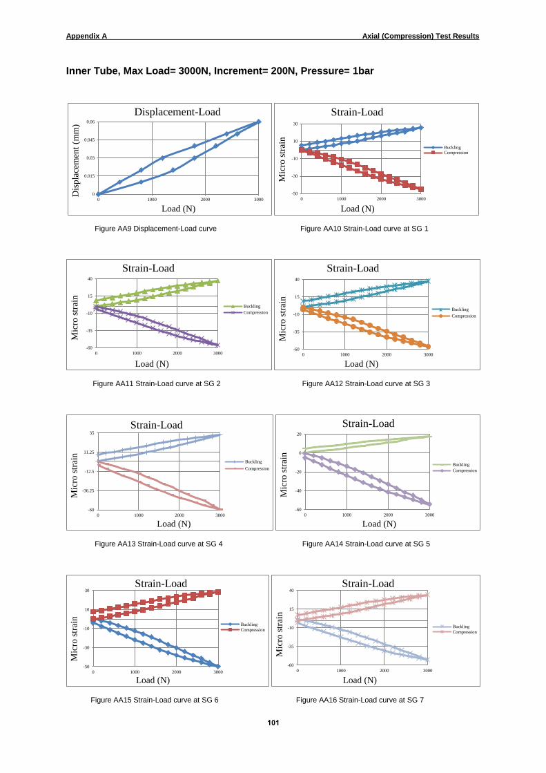
Appendix A Axial (Compression) Test Results
010
Inner Tube, Max Load= 3000N, Increment= 200N, Pressure= 1bar
Figure AA9 Displacement-Load curve Figure AA10 Strain-Load curve at SG 1
Figure AA11 Strain-Load curve at SG 2 Figure AA12 Strain-Load curve at SG 3
Figure AA13 Strain-Load curve at SG 4 Figure AA14 Strain-Load curve at SG 5
Figure AA15 Strain-Load curve at SG 6 Figure AA16 Strain-Load curve at SG 7
0
0.015
0.03
0.045
0.06
0 1000 2000 3000
Dis
pla
cem
ent
(mm
)
Load (N)
Displacement-Load
-50
-30
-10
10
30
0 1000 2000 3000
Mic
ro s
trai
n
Load (N)
Strain-Load
BucklingCompression
-60
-35
-10
15
40
0 1000 2000 3000
Mic
ro s
trai
n
Load (N)
Strain-Load
Buckling
Compression
-60
-35
-10
15
40
0 1000 2000 3000
Mic
ro s
trai
n
Load (N)
Strain-Load
Buckling
Compression
-60
-36.25
-12.5
11.25
35
0 1000 2000 3000
Mic
ro s
trai
n
Load (N)
Strain-Load
Buckling
Compression
-60
-40
-20
0
20
0 1000 2000 3000
Mic
ro s
trai
n
Load (N)
Strain-Load
Buckling
Compression
-50
-30
-10
10
30
0 1000 2000 3000
Mic
ro s
trai
n
Load (N)
Strain-Load
Buckling
Compression
-60
-35
-10
15
40
0 1000 2000 3000
Mic
ro s
trai
n
Load (N)
Strain-Load
Buckling
Compression

Appendix A Axial (Compression) Test Results
012
Inner Tube, Max Load= 3000N, Increment= 200N, Pressure= 5bar
Figure AA17 Displacement-Load curve Figure AA18 Strain-Load at SG 1
Figure AA19 Strain-Load at SG 2 Figure AA20 Strain-Load at SG 3
Figure AA21 Strain-Load at SG 4 Figure AA22 Strain-Load at SG 5
Figure AA23 Strain-Load at SG 6 Figure AA24 Strain-Load at SG 7
0
0.0125
0.025
0.0375
0.05
0 1000 2000 3000Dis
pla
cem
ent
(mm
)
Load (N)
Displacement-Load
-50
-28.75
-7.5
13.75
35
0 1000 2000 3000
Mic
ro s
trai
n
Load (N)
Strain-Load
Buckling
Compression
-65
-36.25
-7.5
21.25
50
0 1000 2000 3000
Mic
ro s
trai
n
Load (N)
Strain-Load
Buckling
Compression
-60
-33.75
-7.5
18.75
45
0 1000 2000 3000
Mic
ro s
trai
n
Load (N)
Strain-Load
Buckling
-65
-48.75
-32.5
-16.25
0
0 1000 2000 3000
Mic
ro s
trai
n
Load (N)
Strain-Load
Compression
-60
-36.25
-12.5
11.25
35
0 1000 2000 3000
Mic
ro s
trai
n
Load (N)
Strain-Load
Buckling
Compression
-60
-33.75
-7.5
18.75
45
0 1000 2000 3000
Mic
ro s
trai
n
Load (N)
Strain-Load
Buckling
Compression
-65
-32.5
0
32.5
65
0 1000 2000 3000
Mic
ro s
trai
n
Load (N)
Strain-Load
Buckling
Compression
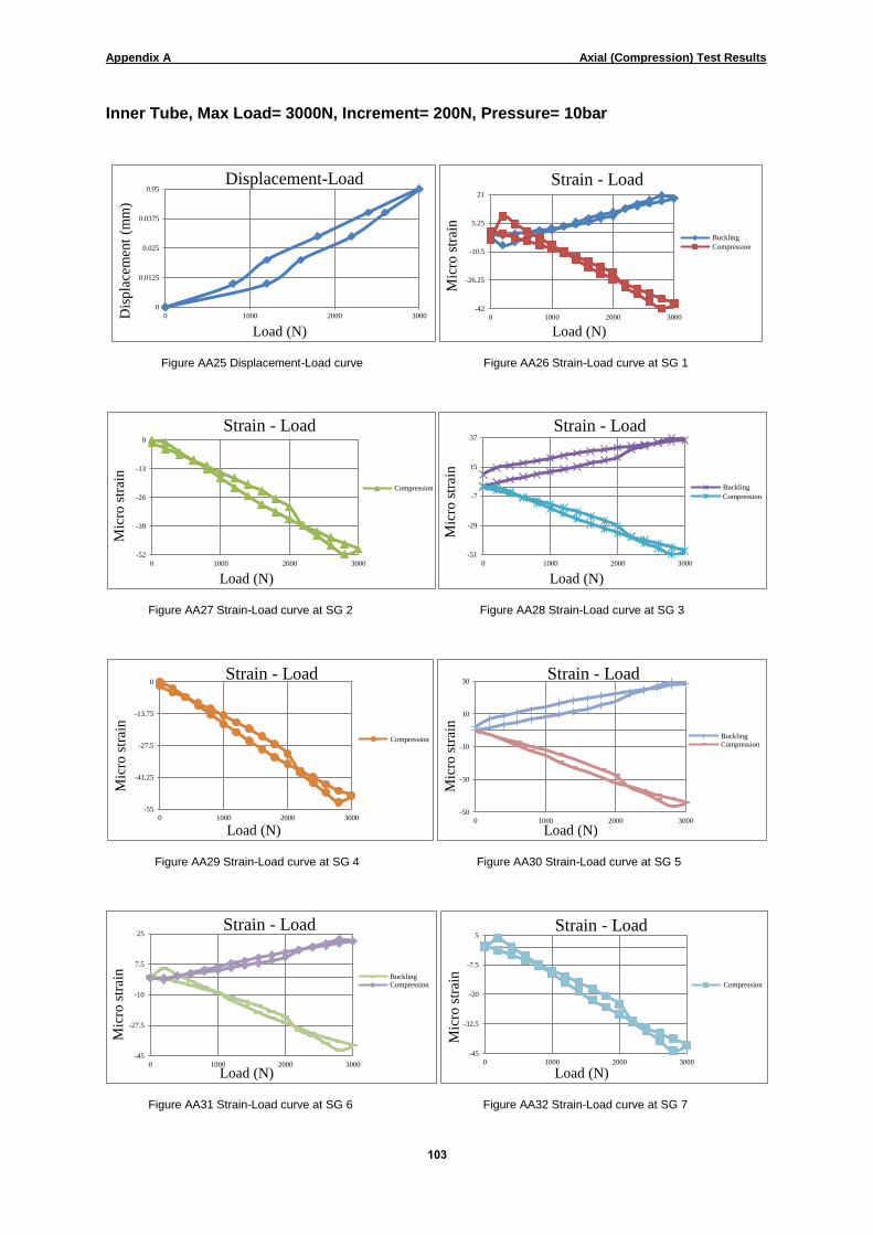
Appendix A Axial (Compression) Test Results
013
Inner Tube, Max Load= 3000N, Increment= 200N, Pressure= 10bar
Figure AA25 Displacement-Load curve Figure AA26 Strain-Load curve at SG 1
Figure AA27 Strain-Load curve at SG 2 Figure AA28 Strain-Load curve at SG 3
Figure AA29 Strain-Load curve at SG 4 Figure AA30 Strain-Load curve at SG 5
Figure AA31 Strain-Load curve at SG 6 Figure AA32 Strain-Load curve at SG 7
0
0.0125
0.025
0.0375
0.05
0 1000 2000 3000Dis
pla
cem
ent
(mm
)
Load (N)
Displacement-Load
-42
-26.25
-10.5
5.25
21
0 1000 2000 3000
Mic
ro s
trai
n
Load (N)
Strain - Load
Buckling
Compression
-52
-39
-26
-13
0
0 1000 2000 3000
Mic
ro s
trai
n
Load (N)
Strain - Load
Compression
-51
-29
-7
15
37
0 1000 2000 3000
Mic
ro s
trai
n
Load (N)
Strain - Load
Buckling
Compression
-55
-41.25
-27.5
-13.75
0
0 1000 2000 3000
Mic
ro s
trai
n
Load (N)
Strain - Load
Compression
-50
-30
-10
10
30
0 1000 2000 3000
Mic
ro s
trai
n
Load (N)
Strain - Load
BucklingCompression
-45
-27.5
-10
7.5
25
0 1000 2000 3000
Mic
ro s
trai
n
Load (N)
Strain - Load
BucklingCompression
-45
-32.5
-20
-7.5
5
0 1000 2000 3000
Mic
ro s
trai
n
Load (N)
Strain - Load
Compression
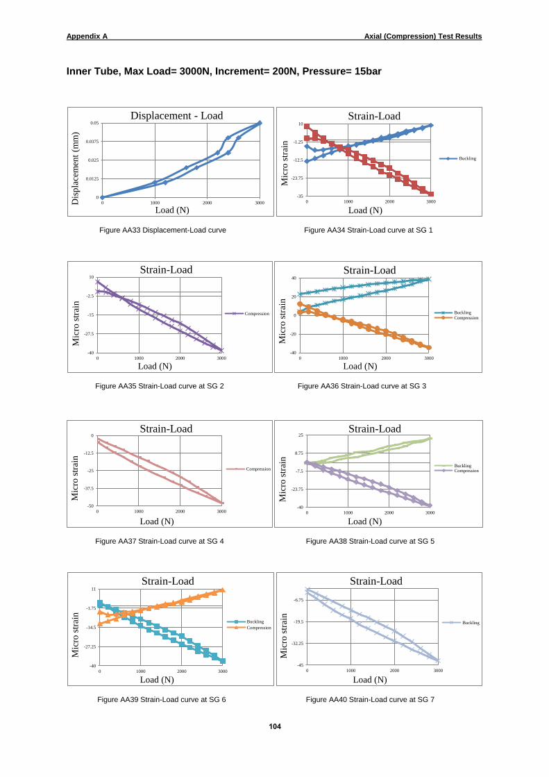
Appendix A Axial (Compression) Test Results
014
Inner Tube, Max Load= 3000N, Increment= 200N, Pressure= 15bar
Figure AA33 Displacement-Load curve Figure AA34 Strain-Load curve at SG 1
Figure AA35 Strain-Load curve at SG 2 Figure AA36 Strain-Load curve at SG 3
Figure AA37 Strain-Load curve at SG 4 Figure AA38 Strain-Load curve at SG 5
Figure AA39 Strain-Load curve at SG 6 Figure AA40 Strain-Load curve at SG 7
0
0.0125
0.025
0.0375
0.05
0 1000 2000 3000Dis
pla
cem
ent
(mm
)
Load (N)
Displacement - Load
-35
-23.75
-12.5
-1.25
10
0 1000 2000 3000
Mic
ro s
trai
n
Load (N)
Strain-Load
Buckling
-40
-27.5
-15
-2.5
10
0 1000 2000 3000
Mic
ro s
trai
n
Load (N)
Strain-Load
Compression
-40
-20
0
20
40
0 1000 2000 3000
Mic
ro s
trai
n
Load (N)
Strain-Load
BucklingCompression
-50
-37.5
-25
-12.5
0
0 1000 2000 3000
Mic
ro s
trai
n
Load (N)
Strain-Load
Compression
-40
-23.75
-7.5
8.75
25
0 1000 2000 3000
Mic
ro s
trai
n
Load (N)
Strain-Load
BucklingCompression
-40
-27.25
-14.5
-1.75
11
0 1000 2000 3000
Mic
ro s
trai
n
Load (N)
Strain-Load
Buckling
Compression
-45
-32.25
-19.5
-6.75
0 1000 2000 3000
Mic
ro s
trai
n
Load (N)
Strain-Load
Buckling
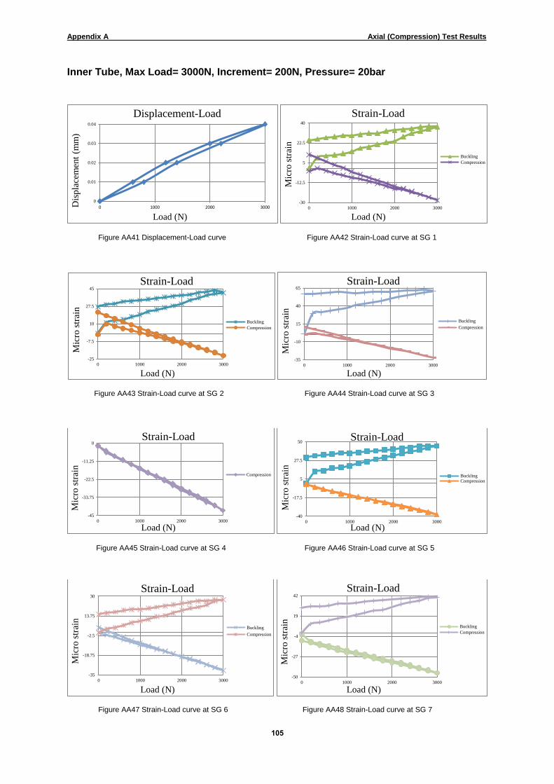
Appendix A Axial (Compression) Test Results
015
Inner Tube, Max Load= 3000N, Increment= 200N, Pressure= 20bar
Figure AA41 Displacement-Load curve Figure AA42 Strain-Load curve at SG 1
Figure AA43 Strain-Load curve at SG 2 Figure AA44 Strain-Load curve at SG 3
Figure AA45 Strain-Load curve at SG 4 Figure AA46 Strain-Load curve at SG 5
Figure AA47 Strain-Load curve at SG 6 Figure AA48 Strain-Load curve at SG 7
0
0.01
0.02
0.03
0.04
0 1000 2000 3000Dis
pla
cem
ent
(mm
)
Load (N)
Displacement-Load
-30
-12.5
5
22.5
40
0 1000 2000 3000
Mic
ro s
trai
n
Load (N)
Strain-Load
Buckling
Compression
-25
-7.5
10
27.5
45
0 1000 2000 3000
Mic
ro s
trai
n
Load (N)
Strain-Load
Buckling
Compression
-35
-10
15
40
65
0 1000 2000 3000
Mic
ro s
trai
n
Load (N)
Strain-Load
Buckling
Compression
-45
-33.75
-22.5
-11.25
0
0 1000 2000 3000
Mic
ro s
trai
n
Load (N)
Strain-Load
Compression
-40
-17.5
5
27.5
50
0 1000 2000 3000
Mic
ro s
trai
n
Load (N)
Strain-Load
BucklingCompression
-35
-18.75
-2.5
13.75
30
0 1000 2000 3000
Mic
ro s
trai
n
Load (N)
Strain-Load
Buckling
Compression
-50
-27
-4
19
42
0 1000 2000 3000
Mic
ro s
trai
n
Load (N)
Strain-Load
Buckling
Compression

Appendix A Axial (Compression) Test Results
016
Inner Tube, No Load, Increasing Pressure effects, Max Pressure= 20 bar
Figure AA49 Displacement-Pressure curve Figure AA50 Strain-Pressure curve at SG 1
Figure AA51 Strain-Pressure curve at SG 2 Figure AA52 Strain-Pressure curve at SG 3
Figure AA53 Strain-Pressure curve at SG 4 Figure AA54 Strain-Pressure curve at SG 5
Figure AA55 Strain-Pressure curve at SG 6 Figure AA56 Strain-Pressure curve at SG 7
-0.02
0.02
0.06
0.1
0.14
0 5 10 15 20
Dis
pla
cem
ent
(mm
)
Pressure (bar)
Displacement-Pressure
-1500
925
3350
5775
8200
0 5 10 15 20
Mic
ro s
trai
n
Pressure (bar)
Strain-Pressure
BucklingCompression
-3000
250
3500
6750
10000
0 5 10 15 20
Mic
ro s
trai
n
Pressure (bar)
Strain-Pressure
Buckling
Compression
-3000
0
3000
6000
9000
0 5 10 15 20
Mic
ro s
trai
n
Pressure (bar)
Strain-Pressure
BucklingCompression
-2600
-1948.75
-1297.5
-646.25
5
0 5 10 15 20
Mic
ro s
trai
n
Pressure (bar)
Strain-Pressure
Compression
-3000
0
3000
6000
9000
0 5 10 15 20
Mic
ro s
trai
n
Pressure (bar)
Strain-Pressure
Buckling
Compression
-3000
0
3000
6000
9000
0 5 10 15 20
Mic
ro s
trai
n
Pressure (bar)
Strain-Pressure
Buckling
Compression
-3000
250
3500
6750
10000
0 5 10 15 20
Mic
ro s
trai
n
Pressure (bar)
Strain-Pressure
Buckling
Compression
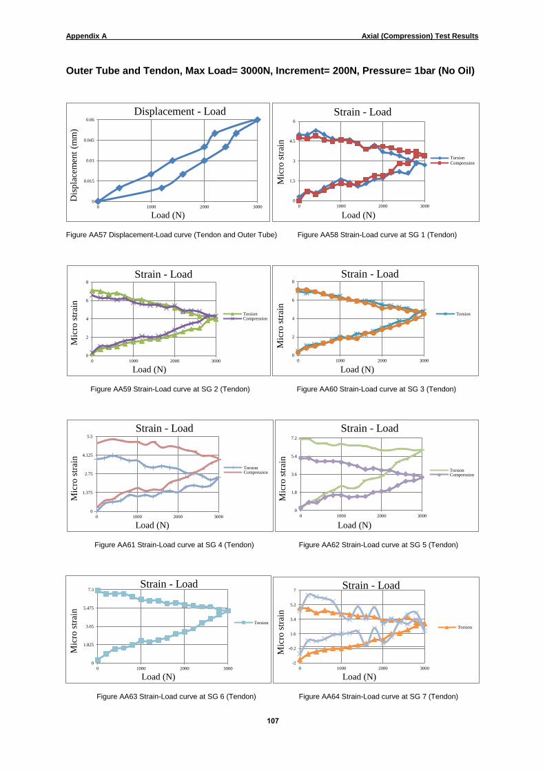
Appendix A Axial (Compression) Test Results
017
Outer Tube and Tendon, Max Load= 3000N, Increment= 200N, Pressure= 1bar (No Oil)
Figure AA57 Displacement-Load curve (Tendon and Outer Tube) Figure AA58 Strain-Load curve at SG 1 (Tendon)
Figure AA59 Strain-Load curve at SG 2 (Tendon) Figure AA60 Strain-Load curve at SG 3 (Tendon)
Figure AA61 Strain-Load curve at SG 4 (Tendon) Figure AA62 Strain-Load curve at SG 5 (Tendon)
Figure AA63 Strain-Load curve at SG 6 (Tendon) Figure AA64 Strain-Load curve at SG 7 (Tendon)
0
0.015
0.03
0.045
0.06
0 1000 2000 3000
Dis
pla
cem
ent
(mm
)
Load (N)
Displacement - Load
0
1.5
3
4.5
6
0 1000 2000 3000
Mic
ro s
trai
n
Load (N)
Strain - Load
TorsionCompression
0
2
4
6
8
0 1000 2000 3000
Mic
ro s
trai
n
Load (N)
Strain - Load
TorsionCompression
0
2
4
6
8
0 1000 2000 3000
Mic
ro s
trai
n
Load (N)
Strain - Load
Torsion
0
1.375
2.75
4.125
5.5
0 1000 2000 3000
Mic
ro s
trai
n
Load (N)
Strain - Load
TorsionCompression
0
1.8
3.6
5.4
7.2
0 1000 2000 3000
Mic
ro s
trai
n
Load (N)
Strain - Load
TorsionCompression
0
1.825
3.65
5.475
7.3
0 1000 2000 3000
Mic
ro s
trai
n
Load (N)
Strain - Load
Torsion
-2
-0.2
1.6
3.4
5.2
7
0 1000 2000 3000
Mic
ro s
trai
n
Load (N)
Strain - Load
Torsion

Appendix A Axial (Compression) Test Results
018
Figure AA65 Strain-Load curve at SG 1 (Outer Tube) Figure AA66 Strain-Load curve at SG 2 (Outer Tube)
Figure AA67 Strain-Load curve at SG 3 (Outer Tube) Figure AA68 Strain-Load curve at SG 4 (Outer Tube)
Figure AA69 Strain-Load curve at SG 5 (Outer Tube) Figure AA70 Strain-Load curve at SG 6 (Outer Tube)
Figure AA71 Strain-Load curve at SG 7 (Outer Tube)
-12
-3.5
5
13.5
22
0 1000 2000 3000
Mic
ro s
trai
n
Load (N)
Strain - Load
BucklingCompression
-25
-12.25
0.5
13.25
26
0 1000 2000 3000
Mic
ro s
trai
n
Load (N)
Strain - Load
BucklingCompression
-45
-26.25
-7.5
11.25
30
0 1000 2000 3000
Mic
ro s
trai
n
Load (N)
Strain - Load
Buckling
-60
-36.25
-12.5
11.25
35
0 1000 2000 3000
Mic
ro s
trai
n
Load (N)
Strain - Load
Buckling
-70
-40
-10
20
50
0 1000 2000 3000
Mic
ro s
trai
n
Load (N)
Strain - Load
TorsionCompression
-70
-40
-10
20
50
0 1000 2000 3000
Mic
ro s
trai
n
Load (N)
Strain - Load
TorsionCompression
-65
-37.5
-10
17.5
45
0 1000 2000 3000
Mic
ro s
trai
n
Load (N)
Strain - Load
Torsion

Appendix A Axial (Compression) Test Results
019
Outer Tube and Tendon, Max Load= 3000N, Increment= 200N, Pressure= 1bar
Figure AA72 Displacement-Load curve (Tendon and Outer Tube) Figure AA73 Strain-Load curve at SG 1 (Tendon)
Figure AA74 Strain-Load curve at SG 2 (Tendon) Figure AA75 Strain-Load curve at SG 3 (Tendon)
Figure AA76 Strain-Load curve at SG 4 (Tendon) Figure AA77 Strain-Load curve at SG 5 (Tendon)
Figure AA78 Strain-Load curve at SG 6 (Tendon) Figure AA79 Strain-Load curve at SG 7 (Tendon)
0
0.0175
0.035
0.0525
0.07
0 1000 2000 3000
Dis
pla
cem
ent
(mm
)
Load (N)
Displacement - Load
-0.2
0.45
1.1
1.75
2.4
0 1000 2000 3000
Mic
ro s
trai
n
Load (N)
Strain - Load
Torsion
Compression
0
0.625
1.25
1.875
2.5
0 1000 2000 3000
Mic
ro s
trai
n
Load (N)
Strain - Load
Torsion
Compression
-0.4
0.375
1.15
1.925
2.7
0 1000 2000 3000
Mic
ro s
trai
n
Load (N)
Strain - Load
Torsion
Compression
0
0.75
1.5
2.25
3
0 1000 2000 3000
Mic
ro s
trai
n
Load (N)
Strain - Load
TorsionCompression
0
0.675
1.35
2.025
2.7
0 1000 2000 3000
Mic
ro s
trai
n
Load (N)
Strain - Load
Torsion
0
0.65
1.3
1.95
2.6
0 1000 2000 3000
Mic
ro s
trai
n
Load (N)
Strain - Load
Torsion
-2
-1.075
-0.15
0.775
1.7
0 1000 2000 3000
Mic
ro s
trai
n
Load (N)
Strain - Load
Torsion
Compression

Appendix A Axial (Compression) Test Results
001
Figure AA80 Strain-Load curve at SG 1 (Outer Tube) Figure AA81 Strain-Load curve at SG 2 (Outer Tube)
Figure AA82 Strain-Load curve at SG 3 (Outer Tube) Figure AA83 Strain-Load curve at SG 4 (Outer Tube)
Figure AA84 Strain-Load curve at SG 5 (Outer Tube) Figure AA85 Strain-Load curve at SG 6 (Outer Tube)
Figure AA86 Strain-Load curve at SG 7 (Outer Tube)
-25
-15
-5
5
15
0 1000 2000 3000
Mic
ro s
trai
n
Load (N)
Strain - Load
Buckling
Compression
-35
-21.25
-7.5
6.25
20
0 1000 2000 3000
Mic
ro s
trai
n
Load (N)
Strain - Load
Buckling
Compression
-55
-33.75
-12.5
8.75
30
0 1000 2000 3000
Mic
ro s
trai
n
Load (N)
Strain - Load
Buckling
Compression
-70
-43.75
-17.5
8.75
35
0 1000 2000 3000
Mic
ro s
trai
n
Load (N)
Strain - Load
Buckling
Compression
-85
-52.5
-20
12.5
45
0 1000 2000 3000
Mic
ro s
trai
n
Load (N)
Strain - Load
Buckling
Compression
-85
-52.5
-20
12.5
45
0 1000 2000 3000
Mic
ro s
trai
n
Load (N)
Strain - Load
Buckling
Compression
-76
-45.75
-15.5
14.75
45
0 1000 2000 3000
Mic
ro s
trai
n
Load (N)
Strain - Load
Buckling
Compression

Appendix A Axial (Compression) Test Results
000
Outer Tube and Tendon, Max Load= 3000N, Increment= 200N, Pressure= 5bar
Figure AA87 Displacement-Load curve (Tendon and Outer Tube) Figure AA88 Strain-Load curve at SG 1 (Tendon)
Figure AA89 Strain-Load curve at SG 2 (Tendon) Figure AA90 Strain-Load curve at SG 3 (Tendon)
Figure AA91 Strain-Load curve at SG 4 (Tendon) Figure AA92 Strain-Load curve at SG 5 (Tendon)
Figure AA93 Strain-Load curve at SG 6 (Tendon) Figure AA94 Strain-Load curve at SG 7 (Tendon)
0
0.015
0.03
0.045
0.06
0 1000 2000 3000Dis
pla
cem
ent
(m
m)
Load (N)
Displacement - Load
-1.5
-0.875
-0.25
0.375
1
0 1000 2000 3000
Mic
ro s
trai
n
Load (N)
Strain - Load
Torsion
Compression
-0.2
0.3
0.8
1.3
1.8
0 1000 2000 3000
Mic
ro s
trai
n
Load (N)
Strain - Load
Torsion
Compression
0.2
0.625
1.05
1.475
1.9
0 1000 2000 3000
Mic
ro s
trai
n
Load (N)
Strain - Load
TorsionCompression
-0.6
-0.25
0.1
0.45
0.8
0 1000 2000 3000
Mic
ro s
trai
n
Load (N)
Strain - Load
TorsionCompress…
-0.5
0.375
1.25
2.125
3
0 1000 2000 3000
Mic
ro s
trai
n
Load (N)
Strain - Load
TorsionCompression
0
0.775
1.55
2.325
3.1
0 1000 2000 3000
Mic
ro s
trai
n
Load (N)
Strain - Load
Torsion
-2
-1.25
-0.5
0.25
1
0 1000 2000 3000
Mic
ro s
trai
n
Load (N)
Strain - Load
Torsion
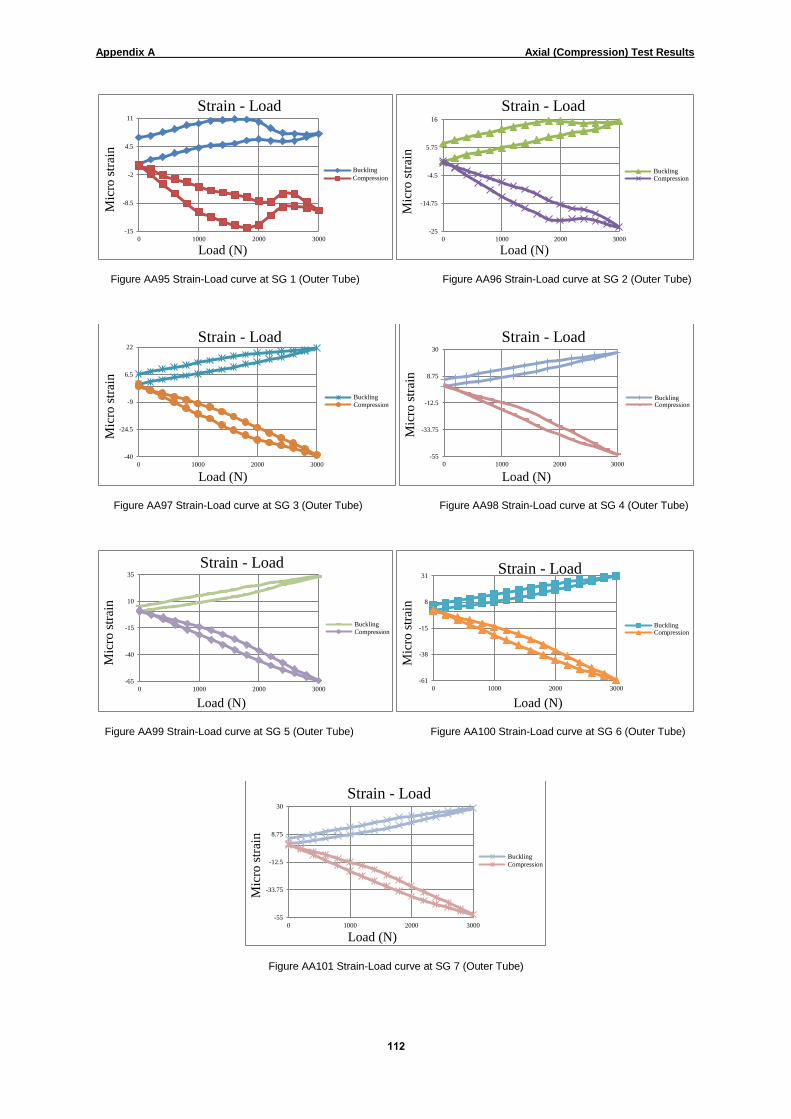
Appendix A Axial (Compression) Test Results
002
Figure AA95 Strain-Load curve at SG 1 (Outer Tube) Figure AA96 Strain-Load curve at SG 2 (Outer Tube)
Figure AA97 Strain-Load curve at SG 3 (Outer Tube) Figure AA98 Strain-Load curve at SG 4 (Outer Tube)
Figure AA99 Strain-Load curve at SG 5 (Outer Tube) Figure AA100 Strain-Load curve at SG 6 (Outer Tube)
Figure AA101 Strain-Load curve at SG 7 (Outer Tube)
-15
-8.5
-2
4.5
11
0 1000 2000 3000
Mic
ro s
trai
n
Load (N)
Strain - Load
Buckling
Compression
-25
-14.75
-4.5
5.75
16
0 1000 2000 3000
Mic
ro s
trai
n
Load (N)
Strain - Load
BucklingCompression
-40
-24.5
-9
6.5
22
0 1000 2000 3000
Mic
ro s
trai
n
Load (N)
Strain - Load
Buckling
Compression
-55
-33.75
-12.5
8.75
30
0 1000 2000 3000
Mic
ro s
trai
n
Load (N)
Strain - Load
BucklingCompression
-65
-40
-15
10
35
0 1000 2000 3000
Mic
ro s
trai
n
Load (N)
Strain - Load
Buckling
Compression
-61
-38
-15
8
31
0 1000 2000 3000
Mic
ro s
trai
n
Load (N)
Strain - Load
BucklingCompression
-55
-33.75
-12.5
8.75
30
0 1000 2000 3000
Mic
ro s
trai
n
Load (N)
Strain - Load
Buckling
Compression

Appendix A Axial (Compression) Test Results
003
Outer Tube and Tendon, Max Load= 3000N, Increment= 200N, Pressure= 10bar
Figure AA102 Displacement-Load curve (Tendon and Outer Tube) Figure AA103 Strain-Load curve at SG 1 (Tendon)
Figure AA104 Strain-Load curve at SG 2 (Tendon) Figure AA105 Strain-Load curve at SG 3 (Tendon)
Figure AA106 Strain-Load curve at SG 4 (Tendon) Figure AA107 Strain-Load curve at SG 5 (Tendon)
Figure AA108 Strain-Load curve at SG 6 (Tendon) Figure AA109 Strain-Load curve at SG 7 (Tendon)
0
0.0125
0.025
0.0375
0.05
0 1000 2000 3000Dis
pla
cem
ent
(mm
)
Load (N)
Displacement - Load
-1.5
-0.75
0
0.75
1.5
0 1000 2000 3000
Mic
ro s
trai
n
Load (N)
Strain - Load
TorsionCompression
-0.7
-0.075
0.55
1.175
1.8
0 1000 2000 3000
Mic
ro s
trai
n
Load (N)
Strain - Load
TorsionCompression
0
0.525
1.05
1.575
2.1
0 1000 2000 3000
Mic
ro s
trai
n
Load (N)
Strain - Load
TorsionCompression
-2
-1.225
-0.45
0.325
1.1
0 1000 2000 3000
Mic
ro s
trai
n
Load (N)
Strain - Load
TorsionCompression
-1
0.525
2.05
3.575
5.1
0 1000 2000 3000
Mic
ro s
trai
n
Load (N)
Strain - Load
TorsionCompression
0
0.4
0.8
1.2
1.6
0 1000 2000 3000
Mic
ro s
trai
n
Load (N)
Strain - Load
Torsion
-2
-1.3
-0.6
0.1
0.8
0 1000 2000 3000
Mic
ro s
trai
n
Load (N)
Strain - Load
TorsionCompression

Appendix A Axial (Compression) Test Results
004
Figure AA110 Strain-Load curve at SG 1 (Outer Tube) Figure AA111 Strain-Load curve at SG 2 (Outer Tube)
Figure AA112 Strain-Load curve at SG 3 (Outer Tube) Figure AA113 Strain-Load curve at SG 4 (Outer Tube)
Figure AA114 Strain-Load curve at SG 5 (Outer Tube) Figure AA115 Strain-Load curve at SG 6 (Outer Tube)
Figure AA116 Strain-Load curve at SG 7 (Outer Tube)
-11
-6.5
-2
2.5
7
0 1000 2000 3000
Mic
ro s
trai
n
Load (N)
Strain - Load
Buckling
-20
-12
-4
4
12
0 1000 2000 3000
Mic
ro s
trai
n
Load (N)
Strain - Load
Buckling
-36
-22.5
-9
4.5
18
0 1000 2000 3000
Mic
ro s
trai
n
Load (N)
Strain - Load
BucklingCompression
-51
-32
-13
6
25
0 1000 2000 3000
Mic
ro s
trai
n
Load (N)
Strain - Load
Buckling
-61
-37.5
-14
9.5
33
0 1000 2000 3000
Mic
ro s
trai
n
Load (N)
Strain - Load
Buckling
-58
-36
-14
8
30
0 1000 2000 3000
Mic
ro s
trai
n
Load (N)
Strain - Load
BucklingCompression
-51
-31.25
-11.5
8.25
28
0 1000 2000 3000
Mic
ro s
trai
n
Load (N)
Strain - Load
BucklingCompression

Appendix A Axial (Compression) Test Results
005
Outer Tube and Tendon, Max Load = 3000 N, Increment = 200 N, Pressure = 15 bar
Figure AA117 Displacement-Load curve (Tendon and Outer Tube) Figure AA118 Strain-Load curve at SG 1 (Tendon)
Figure AA119 Strain-Load curve at SG 2 (Tendon) Figure AA120 Strain-Load curve at SG 3 (Tendon)
Figure AA121 Strain-Load curve at SG 4 (Tendon) Figure AA122 Strain-Load curve at SG 5 (Tendon)
Figure AA123 Strain-Load curve at SG 6 (Tendon) Figure AA124 Strain-Load curve at SG 7 (Tendon)
0
0.0125
0.025
0.0375
0.05
0 1000 2000 3000Dis
pla
cem
ent
(mm
)
Load (N)
Displacement - Load
-1.6
-0.725
0.15
1.025
1.9
0 1000 2000 3000
Mic
ro s
trai
n
Load (N)
Strain - Load
Torsion
-0.2
0.45
1.1
1.75
2.4
0 1000 2000 3000
Mic
ro s
trai
n
Load (N)
Strain - Load
Torsion
0
0.4
0.8
1.2
1.6
0 1000 2000 3000
Mic
ro s
trai
n
Load (N)
Strain - Load
TorsionCompression
-2.5
-1.5
-0.5
0.5
1.5
0 1000 2000 3000
Mic
ro s
trai
n
Load (N)
Strain - Load
TorsionCompression
-0.7
0.275
1.25
2.225
3.2
0 1000 2000 3000
Mic
ro s
trai
n
Load (N)
Strain - Load
TorsionCompression
-1
-0.55
-0.1
0.35
0.8
0 1000 2000 3000
Mic
ro s
trai
n
Load (N)
Strain - Load
Torsion
-2
-1
0
1
2
0 1000 2000 3000
Mic
ro s
trai
n
Load (N)
Strain - Load
Torsion
Compression

Appendix A Axial (Compression) Test Results
006
Figure AA125 Strain-Load curve at SG 1 (Outer Tube) Figure AA126 Strain-Load curve at SG 2 (Outer Tube)
Figure AA127 Strain-Load curve at SG 3 (Outer Tube) Figure AA128 Strain-Load curve at SG 4 (Outer Tube)
Figure AA129 Strain-Load curve at SG 5 (Outer Tube) Figure AA130 Strain-Load curve at SG 6 (Outer Tube)
Figure AA131 Strain-Load curve at SG 7 (Outer Tube)
-12
-6.25
-0.5
5.25
11
0 1000 2000 3000
Mic
ro s
trai
n
Load (N)
Strain - Load
BucklingCompression
-17
-10.25
-3.5
3.25
10
0 1000 2000 3000
Mic
ro s
trai
n
Load (N)
Strain - Load
BucklingCompression
-35
-21.25
-7.5
6.25
20
0 1000 2000 3000
Mic
ro s
trai
n
Load (N)
Strain - Load
BucklingCompression
-50
-31.25
-12.5
6.25
25
0 1000 2000 3000
Mic
ro s
trai
n
Load (N)
Strain - Load
BucklingCompression
-60
-37.5
-15
7.5
30
0 1000 2000 3000
Mic
ro s
trai
n
Load (N)
Strain - Load
BucklingCompression
-55
-33.75
-12.5
8.75
30
0 1000 2000 3000
Mic
ro s
trai
n
Load (N)
Strain - Load
BucklingCompression
-45
-27.5
-10
7.5
25
0 1000 2000 3000
Mic
ro s
trai
n
Load (N)
Strain - Load
BucklingCompression

Appendix A Axial (Compression) Test Results
007
Outer Tube and Tendon, Max Load= 3000N, Increment= 200N, Pressure= 20bar
Figure AA132 Displacement-Load curve (Tendon and Outer Tube) Figure AA133 Strain-Load curve at SG 1 (Tendon)
Figure AA134 Strain-Load curve at SG 2 (Tendon) Figure AA135 Strain-Load curve at SG 3 (Tendon)
Figure AA136 Strain-Load curve at SG 4 (Tendon) Figure AA137 strain-Load curve at SG 5 (Tendon)
Figure AA138 Strain-Load curve at SG 6 (Tendon) Figure AA139 Strain-Load curve at SG 7 (Tendon)
0
0.0125
0.025
0.0375
0.05
0 1000 2000 3000Dis
pla
cem
ent
(mm
)
Load (N)
Displacement - Load
-3
-1.75
-0.5
0.75
2
0 1000 2000 3000
Mic
ro s
trai
n
Load (N)
Strain - Load
Torsion
-2.3
-1.05
0.2
1.45
2.7
0 1000 2000 3000
Mic
ro s
trai
n
Load (N)
Strain - Load
Torsion
-2
-1
0
1
2
0 1000 2000 3000
Mic
ro s
trai
n
Load (N)
Strain - Load
Torsion
-2.5
-1.625
-0.75
0.125
1
0 1000 2000 3000
Mic
ro s
trai
n
Load (N)
Strain - Load
TorsionCompression
-2.5
-1.5
-0.5
0.5
1.5
0 1000 2000 3000
Mic
ro s
trai
n
Load (N)
Strain - Load
Torsion
-4
-3
-2
-1
0
0 1000 2000 3000
Mic
ro s
trai
n
Load (N)
Strain - Load
Torsion
-3.5
-2
-0.5
1
2.5
0 1000 2000 3000
Mic
ro s
trai
n
Load (N)
Strain - Load
TorsionCompression

Appendix A Axial (Compression) Test Results
008
Figure AA140 Strain-Load curve at SG 1 (Outer Tube) Figure AA141 Strain-Load curve at SG 2 (Outer Tube)
Figure AA142 Strain-Load curve at SG 3 (Outer Tube) Figure AA143 Strain-Load curve at SG 4 (Outer Tube)
Figure AA144 Strain-Load curve at SG 5 (Outer Tube) Figure AA145 Strain-Load curve at SG 6 (Outer Tube)
Figure AA146 Strain-Load curve at SG 7 (Outer Tube)
-10
-3.75
2.5
8.75
15
0 1000 2000 3000
Mic
ro s
trai
n
Load (N)
Strain - Load
BucklingCompression
-10
-3.75
2.5
8.75
15
0 1000 2000 3000
Mic
ro s
trai
n
Load (N)
Strain - Load
BucklingCompress…
-27
-16.5
-6
4.5
15
0 1000 2000 3000
Mic
ro s
trai
n
Load (N)
Strain - Load
Buckling
-45
-27.5
-10
7.5
25
0 1000 2000 3000
Mic
ro s
trai
n
Load (N)
Strain - Load
BucklingCompression
-53
-32.75
-12.5
7.75
28
0 1000 2000 3000
Mic
ro s
trai
n
Load (N)
Strain - Load
Buckling
-50
-30
-10
10
30
0 1000 2000 3000
Mic
ro s
trai
n
Load (N)
Strain - Load
Buckling
-40
-23.75
-7.5
8.75
25
0 1000 2000 3000
Mic
ro s
trai
n
Load (N)
Strain - Load
Buckling
Compression
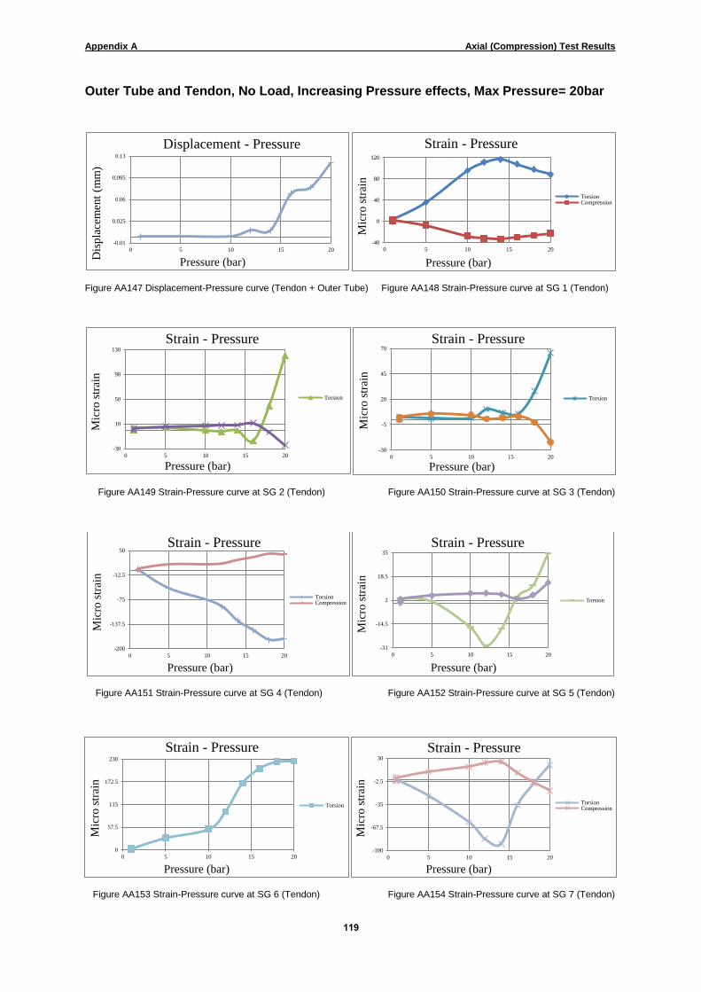
Appendix A Axial (Compression) Test Results
009
Outer Tube and Tendon, No Load, Increasing Pressure effects, Max Pressure= 20bar
Figure AA147 Displacement-Pressure curve (Tendon + Outer Tube) Figure AA148 Strain-Pressure curve at SG 1 (Tendon)
Figure AA149 Strain-Pressure curve at SG 2 (Tendon) Figure AA150 Strain-Pressure curve at SG 3 (Tendon)
Figure AA151 Strain-Pressure curve at SG 4 (Tendon) Figure AA152 Strain-Pressure curve at SG 5 (Tendon)
Figure AA153 Strain-Pressure curve at SG 6 (Tendon) Figure AA154 Strain-Pressure curve at SG 7 (Tendon)
-0.01
0.025
0.06
0.095
0.13
0 5 10 15 20
Dis
pla
cem
ent
(mm
)
Pressure (bar)
Displacement - Pressure
-40
0
40
80
120
0 5 10 15 20
Mic
ro s
trai
n
Pressure (bar)
Strain - Pressure
TorsionCompression
-30
10
50
90
130
0 5 10 15 20
Mic
ro s
trai
n
Pressure (bar)
Strain - Pressure
Torsion
-30
-5
20
45
70
0 5 10 15 20
Mic
ro s
trai
n
Pressure (bar)
Strain - Pressure
Torsion
-200
-137.5
-75
-12.5
50
0 5 10 15 20
Mic
ro s
trai
n
Pressure (bar)
Strain - Pressure
TorsionCompression
-31
-14.5
2
18.5
35
0 5 10 15 20
Mic
ro s
trai
n
Pressure (bar)
Strain - Pressure
Torsion
0
57.5
115
172.5
230
0 5 10 15 20
Mic
ro s
trai
n
Pressure (bar)
Strain - Pressure
Torsion
-100
-67.5
-35
-2.5
30
0 5 10 15 20
Mic
ro s
trai
n
Pressure (bar)
Strain - Pressure
TorsionCompression

Appendix A Axial (Compression) Test Results
021
Figure AA155 Strain-Pressure curve at SG 1 (Outer tube) Figure AA156 Strain-Pressure curve at SG 2 (Outer Tube)
Figure AA157 Strain-Pressure curve at SG 3 (Outer Tube) Figure AA158 Strain-Pressure curve at SG 4 (Outer Tube)
Figure AA159 Strain-Pressure curve at SG 5 (Outer Tube) Figure AA160 Strain-Pressure curve at SG 6 (Outer Tube)
Figure AA161 Strain-Pressure curve at SG 7 (Outer Tube)
-150
-45
60
165
270
0 5 10 15 20
Mic
ro s
trai
n
Pressure (bar)
Strain - Pressure
Buckling
Compression
-50
12.5
75
137.5
200
0 5 10 15 20
Mic
ro s
trai
n
Pressure (bar)
Strain - Pressure
Buckling
Compression
-30
17.5
65
112.5
160
0 5 10 15 20
Mic
ro s
trai
n
Pressure (bar)
Strain - Pressure
BucklingCompression
-160
-80
0
80
160
0 5 10 15 20
Mic
ro s
trai
n
Pressure (bar)
Strain - Pressure
BucklingCompression
-150
-85
-20
45
110
0 5 10 15 20
Mic
ro s
trai
n
Pressure (bar)
Strain - Pressure
BucklingCompression
-170
-85
0
85
170
0 5 10 15 20
Mic
ro s
trai
n
Pressure (bar)
Strain - Pressure
Buckling
-200
-97.5
5
107.5
210
0 5 10 15 20
Mic
ro s
trai
n
Pressure (bar)
Strain - Pressure
BucklingCompression

Appendix B
Blueprints and 3D view of
Components

Appendix B Blueprints and 3D view of Components
022
In this section, blueprints and three-dimensional views of the prototype layers and other
components designed to keep the layers in right place, to seal the prototype when
necessary, or to apply the external load are shown. These components are:
(1) Outer Tube: designed similar to outer sheath layer in real flexible risers, covered all
other layers of the prototype, and was made of clear poly-carbonate (see figure AB1).
(2) Single Helical Armour (or Tendon): was covered by outer sheath and surrounded the
inner cylinder and the material used was CR4 steel (figures AB2 to AB4).
(3) Inner Tube: was made of clear poly-carbonate similar to outer tube, yet it was designed
more accurately in order to seal the pressurized oil inside it; this layer was placed inside
tendon and covered carcass (figure AB5).
(4) Helical Carcass: was made of CR4 yet had more pitch comparing to tendon layer, was
placed inside the inner tube (figure AB6).
(5) End-Caps: were designed to keep the layers of test specimen in desired position, to
help other components seal the fluid inside inner-tube, and to help applying load; they
were installed at each end of the specimen (figures AB7 to AB10).
(6) Threaded Rod: was designed to help the end-caps keep the test layers in place. It was
adjusted by two nuts at its both ends which are sealed by washers and grease (figure
AB11).
(7) Load Part: was designed to apply the external load (figures AB12 to AB14 and AB16).
(8) Bending bed: was designed and made for the bending test; both bending end-caps
were installed on the bed which was installed on loading machine at bottom (magenta in
figure AB15).
A schematic view of total assembly for axial loading is demonstrated in figure AB16.

Appendix B Blueprints and 3D view of Components
023
Figure AB1 Outer tube blueprint
Figure AB2 Tendon blueprint

Appendix B Blueprints and 3D view of Components
024
Figure AB3 Tendon 3D view
Figure AB4 Single tendon testing blueprint
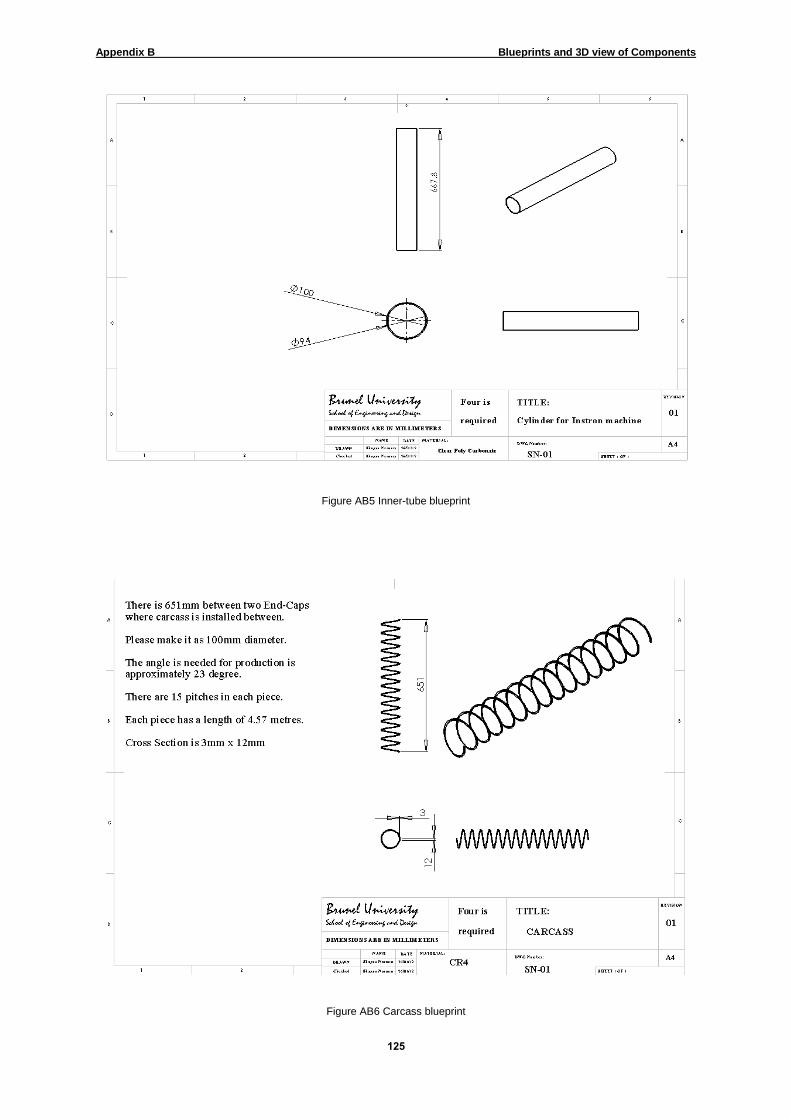
Appendix B Blueprints and 3D view of Components
025
Figure AB5 Inner-tube blueprint
Figure AB6 Carcass blueprint
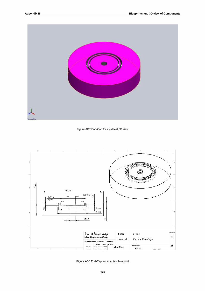
Appendix B Blueprints and 3D view of Components
026
Figure AB7 End-Cap for axial test 3D view
Figure AB8 End-Cap for axial test blueprint

Appendix B Blueprints and 3D view of Components
027
Figure AB9 End-Cap of bending test blueprint 1
Figure AB10 End-Cap of bending test blueprint 2

Appendix B Blueprints and 3D view of Components
028
Figure AB11 Thread rod dimensions blueprint
Figure AB12 Load Part for cyclic loading dimensions blueprint

Appendix B Blueprints and 3D view of Components
029
Figure AB13 Load Part for static loading blueprint
Figure AB14 Load Part for static loading 3D view

Appendix B Blueprints and 3D view of Components
031
Figure AB15 Bending bed blueprint
Figure AB16 Schematic view of axial loading assembly blueprint

Appendix C
Lagrange Multiplier
Method Equations

Appendix C Lagrange Multiplier Method Equations
032
Internal energy term is:
∫ (AC.1)
After using this method, internal energy term augmented form would be:
∫ ∫
(AC.2)
(AC.3)
(AC.4)
(AC.5)
,
[
] {
} {
} (AC.6)

Appendix C Lagrange Multiplier Method Equations
033
∫ ∫ ∫
(AC.7)
(AC.8)
(AC.9)
(AC.10)