1

Nonlinear Adaptive Excitation Control for StructurePreserving Power Systems

Yong Wan, and Federico Milano,Fellow, IEEE

Abstract—The paper proposes a decentralized excitation con-troller to improve the stability of large power systems. ExtendedLyapunov-like energy function and equivalent expressionsofstator transient voltages are utilized to design a nonlinear adap-tive excitation controller. The proposed controller only requireslocal machine measures and parameters. The performance ofthe designed excitation control system is evaluated on the well-known IEEE 118-bus 54-unit power system and compared withconventional exciter controls.

Index Terms—Multi-machine power systems, automatic volt-age control, structure preserving model, transient stability anal-ysis, decentralized control, Lyapunov function.

NOMENCLATURE

SPM Structure preserving model.RNM Reduced-network model.AEC Adaptive excitation controller.RNC RNM-based excitation controller.m Number of machines.b Number of buses.l, k, pjq Index of (machine) bus.Ωl Index set of buses which connect to busl.Ω Index set of branches,k P Ωl ñ lk P Ω.b, pmq Index set of (machine) buses,m Ď b.Z0 Equilibrium value of any variableZ.9Z Time derivative of any variableZ.Hessp¨q Hessian matrix of a function.Vtl Voltage magnitude of busl, in pu.V Voltage magnitude vector.θl Voltage angle of busl, in rad.θ Voltage angle vector.δj Power angle ofjth machine, in rad.δ Power angle vector.δj , θlk Relative anglesδj “ δj ´ θj , θlk “ θl ´ θk.Vdj

, Vqj Vdj“ ´Vtj sin δj , Vqj “ Vtj cos δj .

Vsj , Vcj Vsj “ Vdj0´ Vdj

, Vcj “ Vqj ´ Vqj0 .ωj Relative speed ofjth machine, in rad/s.ω Relative speed vector.

Yong Wan is with the College of Automation Engineering and theJiangsu Key Laboratory of Internet of Things and Control Technologies,Nanjing University of Aeronautics and Astronautics, Nanjing, China. E-mail:wanyong@nuaa.edu.cn, wanyong17007@163.com

Federico Milano is with the School of Electrical and Electronic Engineering,University College Dublin, Belfield, Ireland. E-mail: federico.milano@ucd.ie

Yong Wan is supported by the National Natural Science Foundation ofChina, under Grant No. 61403194 and Grant No. 61473145, and by the Nat-ural Science Foundation of Jiangsu Province, under Grant No. BK20140836.

Federico Milano is supported by the Science Foundation Ireland, underInvestigator Programme Grant No. SFI/15/IA/3074, and by the EuropeanCommunity, under EC Marie Skłodowska-Curie Career Integration GrantNo. PCIG14-GA-2013-630811.

f0 System frequency.ωs Synchronous speedωs “ 2πf0, in rad/s.Sωj

Relative speedSωj“ ωjωs, in pu.

E1dj, E1

qjd- andq-axis stator transient voltages ofjthmachine, in pu.

Edj, Eqj Edj “ E1dj

´ E1dj0

, Eqj “ E1qj

´ E1qj0

.E1

d,E1q d- andq-axis stator transient voltages vector.

EfdjExcitation voltage ofjth machine, in pu.

x Vector“

V T θT δT ωT E1dTE1

qT‰T

.Hj Inertia constant ofjth machine, in s.Dj Damping coefficient ofjth machine, in pu.Pmj

Mechanical power ofjth machine, in pu.Pej , Qej Active and reactive powers generated byjth

machine, in pu.Pe Active power vector.Plk, Qlk Active and reactive powers transmitted on

the line between busl and busk, in pu.PLl

, QLlActive and reactive powers consumed by theload at busl, in pu.

Glk Conductance of the line between busl andbusk, in pu.

Blk, pBshlk q (shunt) susceptance of the line between bus

l and busk, in pu.B1

lk B1lk “ Blk ´Bsh

lk .T 1dj, T

1qj d- and q-axis open circuit transient time

constants ofjth machine, in s.xdj

, xqj d- andq-axis synchronous reactances ofjthmachine, in pu.

x1dj, x1

qjd- and q-axis transient reactances ofjthmachine, in pu.

x2dj, x2

qjx2dj

“ xdj´ x1

dj, x2

qj“ xqj ´ x1

qj.

x1dqj, pj x1

dqj“ x1

dj´ x1

qj, pj “ xdj

pT 1djx

1djx2dj

q.

λ1l, λ2l Unknown bounds of| 9Vtl |x1dl

and | 9θl|x1dl

.c1j Positive constants to be tuned.µ1j , µ2j Positive small constants (ă 1) to be tuned.φdj φdj “

xqj

T 1

qjx1

qj

Vsj ` pωj ´ 9θjqVqj ` 9Vtj sin δj .

φqj φqj “xdj

T 1

djx1

dj

Vcj ` pωj ´ 9θjqVdj` 9Vtj cos δj .

ψpj ψpj “ Pej Vtj .ψdj ψdj “ Qej Vtj ` Vtj x1

dj.

ψqj ψqj “ Qej Vtj ` Vtj x1qj

.

Sdj Sdj “b

ψ2

pj ` ψ2

dj .

Sqj Sqj “b

ψ2

pj ` ψ2

qj .

αdj αdj “ δj ´ arctan pψpjψdjq.αqj αqj “ δj ´ arctan pψpjψqjq.ϕ1j ϕ1j “ cos δj ` sin δj tanαdj0.

2

ϕ2j ϕ2j “ sin δj ´ cos δj tanαdj0.ϕ3j ϕ3j “ Vdj

` Vqj tanαdj0.ϕ4j ϕ4j “ ϕ1j tanhpEqjϕ1jµ1jq.ϕ5j ϕ5j “ Vtjϕ2j tanhpEqjVtjϕ2jµ2jq.V 1sj V 1

sj “ Vsj tanαdj0.

Ξj Ξj “Dj

ωsω2

j ` pjxdj

x1

dj

E2

qj `x2

qj

T 1

qjx12qj

x2

qj

E2

dj .

Ξ1j Ξ1

j “ Ξj ` pjc1jE2

qj .Θj Θj “ µ1jλ1j ` µ2jλ2j .

I. I NTRODUCTION

H IGH-VOLTAGE transmission systems are complex, in-terconnected systems, whose dynamic response, stability

analysis and control have been object of intense study inthe last century. Due to the large number of equations andconstraints that describe real-world power systems, and theresulting high complexity, most techniques aimed at definingand improving transient stability following large disturbances,are generally based onlimited simplified models[1]–[4]. Byutilizing such simplified models, a number of control tech-nologies are presented to design effective excitation controllers[5]. In fact, in the realistic applications, the more accuratethemodel is, the better performance the designed control systemhas, but also the more challenges one needs to address [6].RNM and SPM are two types of power system models for theexcitation control problem. We will, respectively, discuss theirproperties and relative merits in the following part.

In the existing literature, various RNMs were presentedthrough eliminating the network topology and the loadsbyutilizing the integral manifold method [7], [8] or the singularperturbation approach [9]–[12], or by explicitly solving thepower flow constraints under the constant impedance loadsassumption [13]. The RNMs are a set ofnonlinear ordinarydifferential equations, so the conventional control methodscanbe appliedto obtain many interesting results with the helpof Lyapunov functions, for instance, adaptive backstepping,L2 disturbance attenuation, dynamic surface, neural networkand high-order sliding-mode methods have been utilized todesign robust nonlinear excitation controllers [14]–[20], anda centralized excitation control law has been designed byusing the Hamiltonian function method [21]. Nevertheless,RNMs only include the limited terms related to generatorbuses rather than the whole network buses, i.e., the loadbus voltages are neglected in RNMs. Thus, as pointed outin our aforementioned discussion, the performances of thecorresponding designed excitation control systems may be notsatisfactory in the realistic applications.

Differing from these, the SPM was firstly proposed in [22]and it naturally preserves the physical meanings of powernetwork components. But since the SPM is a set ofnonlineardifferential-algebraic equations, many classical control tech-niques, e.g., backstepping,cannot be applied directly. Onlya few works investigated how to overcome the limit of theSPM-basedtransient stability assessment and control. In [23],[24], the immersion and invariance method has been appliedto a differential algebraic single-machine power system todesign an excitation controller. But as stated in [25], this

Interconnected Network

m+1

b

. . . . . .

( )

( )

~

~

1

m

. . . . . .

,

,

,

,

Fig. 1: An m-machineb-bus structure preserving power system with nonlinear loads.

work neglected the reactive power balance and the consideredmodel was not correct. Besides, there are also other beneficialresults with the key idea of constructingenergy functions. Forexample, in [26]–[28], Lyapunov-like energy functions havebeen constructed to perform transient stability analysis basedon the traditional swing equation dynamic model which isa simplified SPM; and in [29], energy-shaping technologieshave been used to design decentralized excitation controller.However, the existing worksneglect the transient effects ofthe damper winding and the transient saliencywhich aresignificant factors, due to the intrinsic difficulties encounteredin constructing Lyapunov functions and the controller singu-larity problem (see SectionIII-B for further explanation). Inaddition, the fact thatthe dynamic models of bus voltage mag-nitudes and angles and the exact values of SPM parameters,while they also play an important role in transient stabilitystudies, are generally unknown, and this should be consideredin the excitation controller design.

In summary, for transient stability problem, it is necessaryto comprehensively consider the aforementioned factors onthe SPM, and then to tackle the corresponding challenges.Therefore, this paper proposesan extendedLyapunov-like en-ergyfunction anda nonlinearadaptive decentralizedexcitationcontrol strategy to improve transient stability of a structurepreserving power system with nonlinear loads. Comparedwith the previous works, the main features of the proposedcontroller are threefold: (i) the design of the controller is basedon relatively accurate power system model; (ii) only localmachine quantities are needed to design the controller; and(iii)adaptive scheme is given to maintain robustness of excitationsystem even though there are unknown or varying in the SPMparameters involved by sudden and severe disturbances.

The remainder of the paper is organized as follows: Sec-tion II describes a high-order SPM. SectionIII proposes anextended Lyapunov-like energy function. In SectionIV, anonlinear adaptive decentralized excitation controller is de-signed based on the proposed energy function. The controllerevaluation results are presented in SectionV. Conclusions aredrawn in SectionVI.

II. STRUCTURE PRESERVINGMODEL

We consider anm-machineb-bus structure preserving powersystem shown in Figure1. Without loss of generality, thetwo-axis model is utilized for allm machines. The followingnotation is adopted in the remainder of the paper:

3

1. If l R m, thenPel “ Qel “ 0.2. If k R Ωl, thenBlk “ Bsh

lk “ 0.The following models are assumed for the generators,

transmission lines and loads.

A. Generator Model

In this paper, we consider a fourth-order synchronous ma-chine model [3], [4], as follows:

9δj “ ωj,

9ωj “ ´Dj

Hjωj ` ωs

HjpPmj

´ Pej q,

T 1qj

9E1dj

“x2

qj

x1

qj

Vdj´

xqj

x1

qj

E1dj,

T 1dj

9E1qj

“x2

dj

x1

dj

Vqj ´xdj

x1

dj

E1qj

` Efdj,

(1)

Pej “ 1

x1

qj

E1djVqj ´ 1

x1

dj

E1qjVdj

´x1

dqj

x1

djx1

qj

VdjVqj ,

Qej “ 1

x1

qj

E1djVdj

` 1

x1

dj

E1qjVqj ´ 1

x1

qj

V 2

dj´ 1

x1

dj

V 2

qj.

(2)

Note that: The excitation voltageEfdjis equivalently trans-

formed intoEfdj“ Efdj0

`uj, uj is excitation control input.

B. Lossy Network Model

The transmission lines are modeled with the standardlumpedΠ circuit [1]

Plk “ GlkV2

tl` VtlVtkpBlk sin θlk ´Glk cos θlkq,

Qlk “ B1lkV

2

tl´ VtlVtkpBlk cos θlk `Glk sin θlkq.

(3)

C. Load Model

The loads at each bus are represented by the followingarbitrary functions of the voltage and the angle at the bus

PLl“ fplpθlq, QLl

“ fqlpVtlq. (4)

Note that, for the definition of the proposed control scheme,the expression offpl and fql do not need to be knownexplicitly. Finally, load power consumptions are linked tothegrid through well-known power flow equations:

Pl :“ ´Pel ` PLl`řb

k“1Plk “ 0,

Ql :“ p´Qel `QLl`řb

k“1QlkqVtl “ 0.

(5)

III. L YAPUNOV-LIKE ENERGY FUNCTION

In this subsection, we define aLyapunov-like energy func-tion that has a unique minimum on the operating point ofstructure preserving power system model consisting of (1),(2), (3), (4), and (5).

A. Structure Preserving Energy Function

In [30], the nonexistence of an energy function of a lossypower system has been shown. Thus, a necessary conditionfor the success of the energy function method is that thenetwork is assumed to be lossless, i.e.,Glk “ 0. This isa general assumption which has been widely used in powersystems analysis and control [19], [21], [27]–[29], [31], [32].The few attempts to remove the constraintGlk “ 0, appears

to be limited to small examples (see, for example, [33]).We will, hence, assume a lossless transmission system. Note,however, that this assumption does not affect the resultingcontrol scheme, as discussed in the case study.

We consider the following energy function:

Epxq “mÿ

j“1

´

´ Pmjδj `

Hj

2ωs

ω2

j `xqj

2x1qjx2qj

E2

dj

`xdj

2x1djx2dj

E2

qj ´E1

dj0

x1qj

Vdj´E1

qj0

x1dj

Vqj

`x1dj

` x1qj

4x1djx1qj

V 2

tj`

x1dqj

4x1djx1qj

pV 2

dj´ V 2

qjq¯

`bÿ

l“1

bÿ

k“1

´

B1lk

ż Vtl

Vtl0

xldxl ´Blk

2VtlVtk cos θlk

¯

`bÿ

l“1

´

ż Vtl

Vtl0

fqlpxlq

xldxl `

ż θl

θl0

fplpxlqdxl¯

.

(6)

Proposition1. The operating pointx0 is the unique mini-mum of the energy functionE in (6) based on the facts:

BEBx |x“x0

“ 0, (7)

HesspEq |x“x0ą 0. (8)

Proof. See the Appendix.

According to the proposition above,Epxq is a Lyapunov-like energy function.

It is important to note that (6) is not unique. As a matter offact, in the literature, several other energy functions have beenproposed [4]. For example, the following energy function isoften employed to analyze the stability of theopen-looppowersystem (i.e. foruj “ 0):

E1pxq “ Epxq `mÿ

j“1

´E1dj0

x1qj

Vdj`E1

qj0

x1dj

Vqj

`1

x1qj

E1djVsj ´

1

x1dj

E1qjVcj

¯

.

(9)

Proposition2. E1 in (9) satisfies the conditions:

BE1

Bx |x“x0“ 0, (10)

9E1 ď 0. (11)

Proof. See reference [4].

The method proposed in [34] to justify the positive defi-niteness of the Hessian matrix of (9) is computationally verydemanding and, for large systems, it is actually not possibleto decide whetherE1 is a Lyapunov function. This is the mainweakness of the “open-loop” analysis framework and severalother energy functions considered in the literature and themainmotivation for proposing (6). In the remainder of the paper,we will study the nonlinear excitation control synthesis andanalyze the stability of the closed-loop power system basedon the Lyapunov-like energy functionE given in (6).

4

B. Problem Statement

Based on SPM, i.e., (1), (2), (3), (4), (5) and (19) asdescribed in SectionII and in Appendix, respectively, the timederivative ofEpxq along the system trajectory is

9E “řm

j“1

“

´ Ξj ` Eqj

x1

dj

`

φqj `xdj

T 1

djx2

dj

uj˘

´Edj

x1

qj

φdj‰

. (12)

Through the observation of (12), the following remarks consti-tute relevant challenges for the design of the excitation control:

1. It is difficult to cancel the nonlinear function termEdjφdjx1

qjthrough the control inputuj , because of

controller singularity.2. Due to the implicit form ofVtl and θl, the dynamics

9Vtl :“ fvlptq and 9θl :“ fθlptq in eq. (5) are unknown.3. The exact values of power system parameters are known

with a certain degree of uncertainty.

These challenges are addressed in the following section.

IV. EXCITATION CONTROL BASED ONENERGY FUNCTION

From Proposition1 given in SectionIII-A , a natural idea toensure post-fault transient stability is to impose that thetimederivative of the energy functionEpxq is non-positive. Thiscondition is direct consequence of Lyapunov second stabilitymethod. With this aim, in this section, an adaptive decen-tralized control scheme is proposed to solve the difficultiesdiscussed in SectionIII-B .

A. Preliminaries

We first introduce the following two standard assumptionsto make the control synthesis tractable.

Assumption1. The following approximate expressions ofEqj and Edj are used for the control synthesis:

Edjx1qj

.“ ´Eqj tanαdj0x1

dj. (13)

Assumption2. There exist unknown positive constantsλ1l, λ2l such that|fvlptq|x1

dlă λ1l and |fθlptq|x1

dlă λ2l.

Remark 1. Note that, based on (2), and using trianglefunction identities, one can get the following expressions:

E1qj

x1dj

“ Sdj cosαdj ,

E1dj

x1qj

“ ´Sqj sinαqj .(14)

Thus, one can conclude that the values ofE1qj

(E1dj

) dependmuch more onSdj (Sqj) than onαdj (αqj ). Moreover, sincex1dj

.“ x1

qj, thenSdj

.“ Sqj andαdj

.“ αqj . Hence, Assumption

1 is reasonable.

Remark2. As stated in Remark1, Assumption 1 is a con-ventional hypothesis for establishing a relationship betweenEqj and Edj to avoid the singularity problem. In addition,based on power flow equation (5) and the implicit functiontheorem, the time derivatives of implicit algebraic variablespVtj , θjq can be deduced as nonlinear functions of systemvariablesx which are known to be bounded (see [19]) bymeans of various protection schemes such as operating securitylimits. Therefore, the dynamics9Vtl and 9θl are also boundedand Assumption 2 with unknown bounds is reasonable.

Lemma1. The following inequality holds for anyε ą 0

and for anyζ P R

0 ď |ζ| ´ ζ tanhpζεq ď κε, (15)

κ is a constant that satisfiesκ “ e´pκ`1q, i.e. κ “ 0.2785.

Proof. See reference [35].

In the following, Lemma1 will be utilized to process theuncertainties resulting from unknown boundsλ1l and λ2l inthe proposed adaptive control design and analysis.

B. Excitation Controller Design

AEC, for which only local information is needed, is pro-posed as follows.

First, let ϑkjpk “ 1, ..., 5q denote the parametric estimates

and defineϑ1j “ ϑ1j ´x2

dj

x1

dj

, ϑ2j “ ϑ2j ´xqj

T 1

djx2

dj

xdjT 1

qjx1

qj

, ϑ3j “

ϑ3j ´T 1

djx2

dj

xdj

, ϑ4j “ ϑ4j ´λ1j

pj, ϑ5j “ ϑ5j ´

λ2j

pjas the

parameter estimation errors.Then, consider the augmented Lyapunov functionW “ E`

pj

2

ř

5

k“1

řmj“1

ϑ2kj . Invoking (12) and (13), we obtain:

9W “řm

j“1

´

´ Ξj ` pjEqjuj

` pj“

pϑ1j ´ ϑ1jqEqj Vcj ` ϑ1j9ϑ1j

‰

` pj“

pϑ2j ´ ϑ2jqEqj V1sj ` ϑ2j

9ϑ2j

‰

` pj“

pϑ3j ´ ϑ3jqEqjωjϕ3j ` ϑ3j9ϑ3j

‰

` pj“

pϑ4j ´ ϑ4jqEqjϕ4j ` ϑ4j9ϑ4j

‰

` pj“

pϑ5j ´ ϑ5jqEqjϕ5j ` ϑ5j9ϑ5j

‰

`` 9Vtj

x1

dj

Eqjϕ1j ´ λ1jEqjϕ4j

˘

`` 9θj

x1

dj

EqjVtjϕ2j ´ λ2jEqjϕ5j

˘

¯

.

(16)

Finally, the control signaluj , which incorporates adaptiveupdating laws of unknown parameters, is designed as follows:

9ϑ1j “ Eqj Vcj ,

9ϑ2j “ Eqj V

1sj ,

9ϑ3j “ Eqjωjϕ3j ,

9ϑ4j “ Eqjϕ4j ,

9ϑ5j “ Eqjϕ5j ,

φj “ ϑ1j Vcj ` ϑ2j V1sj ` ϑ3jωjϕ3j ,

χj “ ϑ4jϕ4j ` ϑ5jϕ5j ,

uj “ ´pφj ` χj ` c1jEqjq.

(17)

In order to clearly show the above controller, block diagramis given in Figure2. Substituting (17) into (16) and applyingLEMMA 1, we obtain:

9W ăřm

j“1

“

´ Ξ1j ` λ1j

`

|Eqjϕ1j | ´ Eqjϕ4j

˘

` λ2j`

|EqjVtjϕ2j | ´ Eqjϕ5j

˘‰

ďřm

j“1p ´ Ξ1

j ` κΘjq.

(18)

The inequality (18) indicates that the proposed control schemeis stable in the Lyapunov sense.

Remark3. In the post-fault transient, system trajectoriescan deviate from their equilibrium points and lead the term

5

= sin

= cos

-+

+

-

= cos + sin tan

= sin cos tan

= + tan

= tanh

= tanh

,

+

-

= tan

=

=

=

=

=

×

×

×

×

×

×Designed Parameters

--

-

---

Input Variables

Fig. 2: Block diagram of AEC model (17).

+

- Exciter

IEEE Excitation System Model

AEC model

+

, ,,

jth Machine Power Grid

Fig. 3: Schematic view of implementation of AEC model (17).

řmj“1

Ξ1j to be large compared withκ

řmj“1

Θj . Therefore,the designed AEC as shown in (17) provides decreasing ofLyapunov functionW along the post-fault system trajectorysuch that the power system will asymptotically converge tothe regionx ´ x0 ď

b

κřm

j“1Θj with arbitrarily small

constantsµ1j andµ2j .

Remark4. For practical implementation of the proposedadaptive excitation system model, a conventional approachasshown in Figure3 (see [36] for reference) is to add the AECoutput signaluj to the voltage reference set point (VREF ,see [37] for details) to produce an error voltage for theexciter which is equipped onjth generator. In other words,the proposed AEC is actually implemented as an additionalsignal added to the voltage error calculation, i.e., automaticvoltage regulator (AVR) summing input [37]. In steady state,this signaluj is zero. As such, the main structure of theexisting excitation system (AVR) is not altered.

Remark5. There are three parametersc1j , µ1j and µ2j

to be tuned for the AEC ofjth generator. First, choose anyinitial values 0 ă c0

1j , 0 ă µ0

1j ă 1 and 0 ă µ0

2j ă 1.Then, under large disturbance test mode, if large overshootof voltage happens, setc1j “ c1

1j ą c01j , µ1j “ µ1

1j ą µ0

1j

and µ2j “ µ1

2j ą µ0

2j . However, larger values of designedparameters may cause larger oscillation of relative speed,thusa trade-off between voltage and relative speed may have to bemade heuristically.

V. CONTROLLER PERFORMANCEEVALUATION

The IEEE 118-bus 54-unit interconnected power systemshown in Figure4 is utilized to evaluate the performance ofthe proposed AEC. The on-line capacity isP “ 9966 MW,Q “ ´7345 „ 11777 MVAr. The total load isPL “ 4242

MW, QL “ 1438 MVAr. Due to space limitation, systemdata (such as power flow solution, generator parameters, lineconductance and susceptance, etc.) is omitted but the interestedreader can find more details in [1].

All simulations are carried out using MATDYN [38] andMATPOWER [39]. It is important to note that, although the

G

G

G

G

G

G

G

G

G

G

G

G

G

G

G

G

G

G

G

G

G

Fig. 4: IEEE 118-bus system.

AEC model is proposed based on the energy function witha conventional lossless approximation as described in Sec-tion III-A , the simulations are performed using the lossynetwork model as shown in SectionII-B.

The following mean errors are defined as the simulationoutputs to achieve a holistic evaluation.

Snω “ 1

54

ř54

j“1|Sωj

|, V nt “ 1

118

ř118

l“1|Vtl ´ Vtl0 |,

Qne “ 1

54

ř54

j“1|Qej ´Qej0 |, En

fd “ 1

54

ř54

j“1|Efdj

´ Efdj0|.

The performance evaluation of the designed AEC isachieved by comparing with the RNC in [18] and the standardIEEE Type DC1C/AC4C excitation systems [37]. Moreover,throughout the simulation, all 54 machines are assumed to bedriven by turbines with constant mechanical output power andare represented by the fourth order model that includes thetransient effects of damper winding and transient saliency.

There are three points to be explained: (i) the AEC requiresthe measurable relative angle (δj), not each quantity (δj orθj) independently; (ii) (extended) Kalman-filter based dynamicestimators [40], [41] can be employed to estimate theq-axis stator transient voltage (E1

qj) which cannot be measured

directly; and (iii) the AEC does not need prior knowledge ofexact values of power system parameters.

TABLE I: COMPARISONSCHEME

Generator ES Condenser ES S1 S2 S3

AEC AEC

TLO TPSC MFRNC RNC

AC4C DC1C1 ES, TLO, TPSC, and MF mean Excitation System, Transmission

Line Outage, Three-Phase Short-Circuit, and Multiple Faults.

The simulation output variables are chosen as relative rotorspeed (Sωj

), bus voltage magnitude (Vtl ), machine reactivepower (Qej ), excitation voltage (Efdj

) and their mean errors(Sn

ω , V nt , Qn

e , Enfd) defined above, for all 54 machines (@j P

m) and 118 buses (@l P b). In addition, TableI provides thesimulation comparison scheme which is implemented throughthe following 3 scenarios (S1, S2, S3).

6

0 1 2 3Time [s]

-3

-2

-1

0

1R

ela

tive

Sp

ee

d S

ωj [

pu

] ×10-4

(a)

0 1 2 3Time [s]

-3

-2

-1

0

1

Re

lativ

e S

pe

ed

Sω

j [p

u] ×10-4

(b)

0 1 2 3Time [s]

-1

-0.5

0

0.5

1

Re

lativ

e S

pe

ed

Sω

j [p

u] ×10-3

(c)

0 1 2 3Time [s]

0

0.5

1

1.5

Me

an

Err

or

Sωn [

pu

]

×10-4

abc

(d)

Fig. 5: Scenario 1: Relative speeds of 54 synchronous machines.(a) Proposed AEC;(b) RNC; (c) Standard IEEE controllers;(d) Comparison of mean errorSnω .

0 1 2 3Time [s]

0.93

0.96

0.99

1.02

1.05

1.08

Vo

ltag

e V

tl [p

u]

(a)

0 1 2 3Time [s]

0.93

0.96

0.99

1.02

1.05

1.08

Vo

ltag

e V

tl [p

u]

(b)

0 1 2 3Time [s]

0.93

0.96

0.99

1.02

1.05

1.08

Vo

ltag

e V

tl [p

u]

(c)

0 1 2 3Time [s]

0

1

2

3

4

5

Me

an

Err

or

Vtn [

pu

]

×10-3

abc

(d)

Fig. 6: Scenario 1: Voltage magnitudes of 118 Buses.(a) Proposed AEC;(b) RNC; (c) Standard IEEE controllers;(d) Comparison of mean errorV nt .

0 1 2 3Time [s]

-1

-0.5

0

0.5

11.2

Re

act

ive

Po

we

r Q

ej [

pu

]

(a)

0 1 2 3Time [s]

-1

-0.5

0

0.5

11.2

Re

act

ive

Po

we

r Q

ej [

pu

]

(b)

0 1 2 3Time [s]

-1

-0.5

0

0.5

11.2

Re

act

ive

Po

we

r Q

ej [

pu

]

(c)

0 1 2 3Time [s]

0

0.005

0.01

0.015

0.02

0.025

Me

an

Err

or

Qen [

pu

]

abc

(d)

Fig. 7: Scenario 1: Reactive powers of 54 synchronous machines.(a) Proposed AEC;(b) RNC; (c) Standard IEEE controllers;(d) Comparison of mean errorQne .

0 1 2 3Time [s]

0

2

4

6

8

10

12

Exc

itatio

n V

olta

ge

Efd

j [p

u]

(a)

0 1 2 3Time [s]

0

2

4

6

8

10

12

Exc

itatio

n V

olta

ge

Efd

j [p

u]

(b)

0 1 2 3Time [s]

0

2

4

6

8

10

12

Exc

itatio

n V

olta

ge

Efd

j [p

u]

(c)

0 1 2 3Time [s]

0

0.02

0.04

0.06

0.08

Me

an

Err

or

Efdn

[p

u]

abc

(d)

Fig. 8: Scenario 1: Excitation voltages of 54 synchronous machines.(a) Proposed AEC;(b) RNC; (c) Standard IEEE controllers;(d) Comparison of mean errorEnfd.

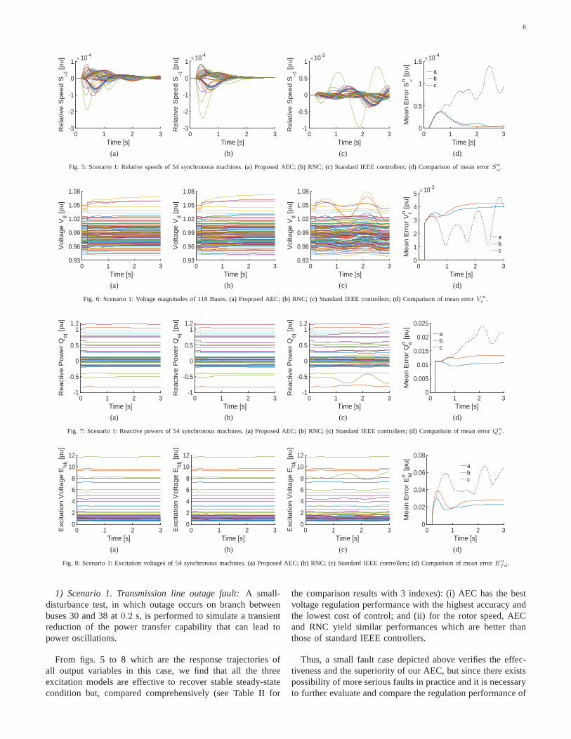
1) Scenario 1. Transmission line outage fault:A small-disturbance test, in which outage occurs on branch betweenbuses 30 and 38 at0.2 s, is performed to simulate a transientreduction of the power transfer capability that can lead topower oscillations.

From figs. 5 to 8 which are the response trajectories ofall output variables in this case, we find that all the threeexcitation models are effective to recover stable steady-statecondition but, compared comprehensively (see TableII for

the comparison results with 3 indexes): (i) AEC has the bestvoltage regulation performance with the highest accuracy andthe lowest cost of control; and (ii) for the rotor speed, AECand RNC yield similar performances which are better thanthose of standard IEEE controllers.

Thus, a small fault case depicted above verifies the effec-tiveness and the superiority of our AEC, but since there existspossibility of more serious faults in practice and it is necessaryto further evaluate and compare the regulation performanceof

7

0 1 2 3Time [s]

-4

-2

0

2

4

6

8R

ela

tive

Sp

ee

d S

ωj [

pu

] ×10-3

(a)

0 1 2 3Time [s]

-4

-2

0

2

4

6

8

Re

lativ

e S

pe

ed

Sω

j [p

u] ×10-3

(b)

0 1 2 3Time [s]

-0.030

0.1

0.2

0.32

Re

lativ

e S

pe

ed

Sω

j [p

u]

(c)

0 1 2 3Time [s]

0

0.01

0.02

0.032

Me

an

Err

or

Sωn [

pu

]

abc

(d)

Fig. 9: Scenario 2: Relative speeds of 54 synchronous machines.(a) Proposed AEC;(b) RNC; (c) Standard IEEE controllers;(d) Comparison of mean errorSnω .

0 1 2 3Time [s]

0

0.2

0.4

0.6

0.8

1

1.2

Vo

ltag

e V

tl [p

u]

(a)

0 1 2 3Time [s]

0

0.2

0.4

0.6

0.8

1

1.2

Vo

ltag

e V

tl [p

u]

(b)

0 1 2 3Time [s]

0

0.33

0.66

1

1.33

1.66

Vo

ltag

e V

tl [p

u]

(c)

0 1 2 3Time [s]

0

0.055

0.11

0.165

Me

an

Err

or

Vtn [

pu

]

abc

(d)

Fig. 10: Scenario 2: Voltage magnitudes of 118 Buses.(a) Proposed AEC;(b) RNC; (c) Standard IEEE controllers;(d) Comparison of mean errorV nt .

0 1 2 3Time [s]

-1.9

0

1.9

3.8

Re

act

ive

Po

we

r Q

ej [

pu

]

(a)

0 1 2 3Time [s]

-1.9

0

1.9

3.8

Re

act

ive

Po

we

r Q

ej [

pu

]

(b)

0 1 2 3Time [s]

-9

-6

-3

0

3

6

Re

act

ive

Po

we

r Q

ej [

pu

]

(c)

0 1 2 3Time [s]

0

0.3

0.6

0.9

Me

an

Err

or

Qen [

pu

]

abc

(d)

Fig. 11: Scenario 2: Reactive powers of 54 synchronous machines.(a) Proposed AEC;(b) RNC; (c) Standard IEEE controllers;(d) Comparison of mean errorQne .

0 1 2 3Time [s]

-43

-18

0

18

36

54

Exc

itatio

n V

olta

ge

Efd

j [p

u]

(a)

0 1 2 3Time [s]

-43

-18

0

18

36

54

Exc

itatio

n V

olta

ge

Efd

j [p

u]

(b)

0 1 2 3Time [s]

-43

-18

0

18

36

54

Exc

itatio

n V

olta

ge

Efd

j [p

u]

(c)

0 1 2 3Time [s]

0

1.75

3.5

5.25

7

Me

an

Err

or

Efdn

[p

u] a

bc

(d)

Fig. 12: Scenario 2: Excitation voltages of 54 synchronous machines.(a) Proposed AEC;(b) RNC; (c) Standard IEEE controllers;(d) Comparison of mean errorEnfd.

AEC, we consider a three-phase fault in the next scenario.2) Scenario 2. Three-phase short-circuit fault:A large

disturbance namely three-phase fault that occurs on bus 1 at0.2 s and then is cleared after250 ms, is utilized to furtherevaluate our AEC. During the fault, the synchronous machineat the faulted bus cannot generate active and reactive powernormally, and the voltage at this short-circuit bus will dropto zero. As such, in the post-fault period, if there is no validexcitation control, the fault may trigger critical oscillations andmay eventually lead to the whole system instability.

As shown in figs.9 to 12, the response curves of theoutputs of AEC, RNC, and IEEE standard controllers, whichare obtained by considering this large fault, are compared (seeTable II for further results). Following this: (i) the proposedAEC is able to get the smoothest and the most stable responsesand to regulate the voltages to their desired values in themost accurate way by the lowest costs of reactive powerinjection and field voltage control; (ii) the RNC exhibitssmaller overshoot and steady-state error on the rotor speed

8

0 1 2 3Time [s]

-3

-2

-1

0

1

2

3R

ela

tive

Sp

ee

d S

ωj [

pu

] ×10-3

(a)

0 1 2 3Time [s]

-3

-2

-1

0

1

2

3

Re

lativ

e S

pe

ed

Sω

j [p

u] ×10-3

(b)

0 1 2 3Time [s]

-6.5

-3

0

3

5.5

Re

lativ

e S

pe

ed

Sω

j [p

u] ×10-3

(c)

0 1 2 3Time [s]

0

0.5

1

1.5

Me

an

Err

or

Sωn [

pu

]

×10-3

abc

(d)

Fig. 13: Scenario 3: Relative speeds of 54 synchronous machines.(a) Proposed AEC;(b) RNC; (c) Standard IEEE controllers;(d) Comparison of mean errorSnω .

0 1 2 3Time [s]

0

0.2

0.4

0.6

0.8

1

1.21

Vo

ltag

e V

tl [p

u]

(a)

0 1 2 3Time [s]

0

0.2

0.4

0.6

0.8

1

1.21

Vo

ltag

e V

tl [p

u]

(b)

0 1 2 3Time [s]

0

0.2

0.4

0.6

0.8

1

1.21

Vo

ltag

e V

tl [p

u]

(c)

0 1 2 3Time [s]

0

0.02

0.04

0.06

0.08

Me

an

Err

or

Vtn [

pu

] abc

(d)

Fig. 14: Scenario 3: Voltage magnitudes of 118 Buses.(a) Proposed AEC;(b) RNC; (c) Standard IEEE controllers;(d) Comparison of mean errorV nt .

0 1 2 3Time [s]

-1.5

-1

-0.5

0

0.5

1

1.5

2

Re

act

ive

Po

we

r Q

ej [

pu

]

(a)

0 1 2 3Time [s]

-1.5

-1

-0.5

0

0.5

1

1.5

2

Re

act

ive

Po

we

r Q

ej [

pu

]

(b)

0 1 2 3Time [s]

-1.5

-1

-0.5

0

0.5

1

1.5

2

Re

act

ive

Po

we

r Q

ej [

pu

]

(c)

0 1 2 3Time [s]

0

0.05

0.1

0.15

0.2

0.25

Me

an

Err

or

Qen [

pu

] abc

(d)

Fig. 15: Scenario 3: Reactive powers of 54 synchronous machines.(a) Proposed AEC;(b) RNC; (c) Standard IEEE controllers;(d) Comparison of mean errorQne .

0 1 2 3Time [s]

-20

-10

0

10

25

Exc

itatio

n V

olta

ge

Efd

j [p

u]

(a)

0 1 2 3Time [s]

-20

-10

0

10

25

Exc

itatio

n V

olta

ge

Efd

j [p

u]

(b)

0 1 2 3Time [s]

-20

-10

0

10

25

Exc

itatio

n V

olta

ge

Efd

j [p

u]

(c)

0 1 2 3Time [s]

0

2

4

6

Me

an

Err

or

Efdn

[p

u] a

bc

(d)

Fig. 16: Scenario 3: Excitation voltages of 54 synchronous machines.(a) Proposed AEC;(b) RNC; (c) Standard IEEE controllers;(d) Comparison of mean errorEnfd.

responses of only a few machines than the AEC, but the RNCcannot eliminate high-frequency oscillation and over-voltage;and (iii) the system controlled by IEEE AC4C/DC1C, instead,is unstable.

Consequently, in comparison with RNC and IEEE con-trollers, the proposed AEC displays its ability to mitigatethelarge fault effects and to recover system steady-state in a shorttime. In addition, only a single fault is included in each of theabove scenarios, in order to assess the performance of the

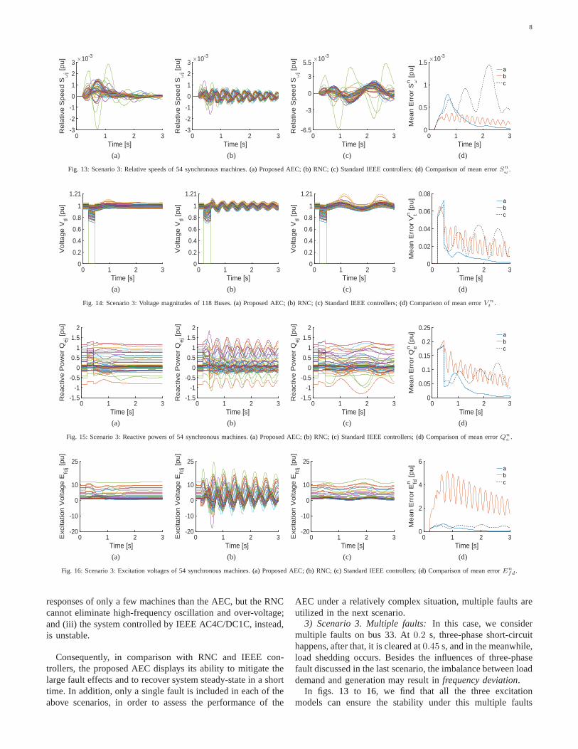
AEC under a relatively complex situation, multiple faults areutilized in the next scenario.

3) Scenario 3. Multiple faults:In this case, we considermultiple faults on bus 33. At0.2 s, three-phase short-circuithappens, after that, it is cleared at0.45 s, and in the meanwhile,load shedding occurs. Besides the influences of three-phasefault discussed in the last scenario, the imbalance betweenloaddemand and generation may result infrequency deviation.

In figs. 13 to 16, we find that all the three excitationmodels can ensure the stability under this multiple faults

9

TABLE II: C OMPARISONRESULTS

Index

Best OutputSωj

Vtj Qej Efdj

OS

S1 * RNC AEC AEC

S2 * AEC AEC AEC

S3 RNC AEC AEC AEC

OFS1 RNC * * *

S2 AEC AEC AEC AEC

S3 AEC AEC AEC AEC

SSES1 RNC AEC AEC AEC

S2 RNC AEC AEC AEC

S3 AEC AEC AEC AEC1 OS, OF and SSE mean Overshoot, Oscillation Frequency

and Steady-State Error respectively.2 * represents both AEC and RNC.

condition, furthermore, as depicted in TableII : (i) for boththe transient process and the steady-state, the AEC exhibitsthe most excellent post-fault voltage regulation by spendingleast costs for reactive power and excitation voltage; and (ii)for the transient process, although AEC has slightly biggeramplitude of the rotor speed responses than RNC, all theoutput trajectories of AEC are more stable than those of RNCand IEEE controllers.

To sum up the above three scenarios, the AEC has adaptabil-ity to different fault conditions and has an outstanding regula-tion performance beyond conventional excitation models. Thisis mainly due to the fact that our AEC is derived based onthe relatively accurate SPM and the proposed extended energyfunction which possesses both Lyapunov characteristic andphysical interpretation. Additionally, the comparison resultsalso confirm the theoretical ones given in the previous section.

VI. CONCLUSION

The paper proposes a nonlinear adaptive excitation con-troller that improves the dynamic response of multi-machinepower systems. The main features of the proposed controllerare: (i) it accounts for high-order structure preserving powersystem models with nonlinear loads; (ii) it requires only localmeasurements and data without prior knowledge of exactSPM parameters; (iii) it uses only four available variablesfor feedback (as discussed in SectionV); and (iv) it includesonly three parameters to be tuned. The results obtained inthe case study show that the proposed controller outperformconventional control schemes and is able to keep the systemstable also in case of large critical disturbances. Future workwill focus on the analysis of the dynamic response of theproposed controller for systems with high penetration ofrenewables and non-synchronous generation.

APPENDIX

PROOF OFPROPOSITION1

Proof. DifferentiatingE leads to:

BEBδj

“ Pej ´ Pmj` 1

x1

dj

EqjVdj´ 1

x1

qj

EdjVqj ,

BEBωj

“Hj

ωsωj,

BEBE1

qj

“xdj

x1

djx2

dj

Eqj ,BE

BE1

dj

“xqj

x1

qjx2

qj

Edj ,

BEBVtl

“

#

Q1lpδl,V , θq, l P m,

QlpV , θq, l R m,

BEBθl

“

#

P 1l pδl,V , θq, l P m,

PlpV , θq, l R m,

(19)

where P 1l “ Pl ` EdlVqlx

1ql

´ EqlVdlx1

dl, Q1

l “ Ql `

EdlVdlpx1

qlVtlq ` EqlVqlpx1

dlVtlq. The expressions shown in

(19) lead to (7).The Hessian matrix ofE, calculated at the operating point,

is as follows:

HesspEq|x“x0“

»

—

—

—

—

–

BPe

BδBPe

BVBPe

Bθ

HxBQf

BδBPf

Bδ

BQf

BVBQf

BθBPf

BVBPf

Bθ

fi

ffi

ffi

ffi

ffi

fl

ˇ

ˇ

ˇ

ˇ

ˇ

ˇ

ˇ

ˇ

ˇ

ˇ

x“x0

,

where Pf “ colpPlq, Qf “ colpQlq, Hx “

diag

diagtHj

ωsu, diagt

xdj

x1

djx2

dj

u, diagtxqj

x1

qjx2

qj

u(

.

From positive definite Jacobian of normal power flow whichcorresponds to local regularity [27], Lemma 1 in [29] andProposition 2 in [31], one can prove (8). Since both conditions(7) and (8) are satisfied, the energy functionE is Lyapunov-like function.

REFERENCES

[1] P. M. Anderson and A. A. Fouad,Power system control and stability,second edition. Wiley-IEEE Press, 2002.

[2] L. L. Grigsby, Power system stability and control, third edition. BocaRaton: CRC Press, Taylor & Francis, 2012.

[3] K. R. Padiyar,Power system dynamics: stability and control, secondedition. Hyderabad: BS publications, 2008.

[4] ——, Structure preserving energy functions in power systems: theoryand applications. CRC Press, 2013.

[5] M. Ilıc, E. Allen, J. J. Chapman, C. A. King, J. H. Lang, and E. Litvinov,“Preventing future blackouts by means of enhanced electricpowersystems control: From complexity to order,”Proceedings of the IEEE,vol. 93, no. 11, pp. 1920–1941, 2005.

[6] Z. Wang, L. Liu, and H. Zhang, “Neural network-based model-freeadaptive fault-tolerant control for discrete-time nonlinear systems withsensor fault,” IEEE Transactions on Systems, Man, and Cybernetics:Systems, 2017.

[7] P. W. Sauer, S. Ahmed-Zaid, and P. V. Kokotovic, “An integral manifoldapproach to reduced order dynamic modeling of synchronous machines,”IEEE Transactions on Power Systems, vol. PS-3, no. 1, pp. 17–23, 1988.

[8] P. V. Kokotovic and P. W. Sauer, “Integral manifold as a tool forreduced-order modeling of nonlinear systems: A synchronous machinecase study,”IEEE Transactions on Circuits and Systems, vol. 36, no. 3,pp. 403–410, 1989.

[9] B. W. Gordon and S. Liu, “A singular perturbation approach formodeling differential-algebraic systems,”Journal of dynamic systems,measurement, and control, vol. 120, no. 4, pp. 541–545, 1998.

[10] B. W. Gordon, “State space modeling of differential-algebraic systemsusing singularly perturbed sliding manifolds,” Ph.D. dissertation, Mas-sachusetts Institute of Technology, 1999.

[11] I. Martınez, A. R. Messina, and V. Vittal, “Normal formanalysisof complex system models: a structure-preserving approach,” IEEETransactions on Power Systems, vol. 22, no. 4, pp. 1908–1915, 2007.

10

[12] C.-C. Chu and H.-D. Chiang, “Constructing analytical energy functionsfor network-preserving power system models,”Circuits, Systems andSignal Processing, vol. 24, no. 4, pp. 363–383, 2005.

[13] W. Dib, A. E. Barabanov, R. Ortega, and F. Lamnabhi-Lagarrigue, “Anexplicit solution of the power balance equations of structure preservingpower system models,”IEEE Transactions on Power Systems, vol. 24,no. 2, pp. 759–765, 2009.

[14] R. Yan, Z. Y. Dong, T. K. Saha, and R. Majumder, “A power systemnonlinear adaptive decentralized controller design,”Automatica, vol. 46,no. 2, pp. 330–336, 2010.

[15] T. K. Roy, M. A. Mahmud, W. Shen, A. M. T. Oo, and M. E. Haque,“Robust nonlinear adaptive backstepping excitation controller designfor rejecting external disturbances in multimachine powersystems,”International Journal of Electrical Power & Energy Systems, vol. 84,pp. 76–86, 2017.

[16] Y. Wan and B. Jiang, “Practical nonlinear excitation control for asingle-machine infinite-bus power system based on a detailed model,”Automatica, vol. 62, pp. 18–25, 2015.

[17] Y. Wang, D. Cheng, C. Li, and Y. Ge, “Dissipative Hamiltonianrealization and energy-basedL2-disturbance attenuation control of mul-timachine power systems,”IEEE Transactions on Automatic Control,vol. 48, no. 8, pp. 1428–1433, 2003.

[18] H. Liu, Z. Hu, and Y. Song, “Lyapunov-based decentralized excitationcontrol for global asymptotic stability and voltage regulation of multi-machine power systems,”IEEE Transactions on Power Systems, vol. 27,no. 4, pp. 2262–2270, 2012.

[19] S. Mehraeen, S. Jagannathan, and M. L. Crow, “Power system stabi-lization using adaptive neural network-based dynamic surface control,”IEEE Transactions on Power Systems, vol. 26, no. 2, pp. 669–680, 2011.

[20] H. Huerta, A. G. Loukianov, and J. M. Canedo, “Robust multimachinepower systems control via high order sliding modes,”Electric PowerSystems Research, vol. 81, no. 7, pp. 1602–1609, 2011.

[21] W. Dib, R. Ortega, A. Barabanov, and F. Lamnabhi-Lagarrigue, “Aglobally convergent controller for multi-machine power systems usingstructure-preserving models,”IEEE Transactions on Automatic Control,vol. 54, no. 9, pp. 2179–2185, 2009.

[22] A. R. Bergen and D. J. Hill, “A structure preserving model for powersystem stability analysis,”IEEE Transactions on Power Apparatus andSystems, vol. PAS-100, no. 1, pp. 25–35, 1981.

[23] N. S. Manjarekar, R. N. Banavar, and R. Ortega, “An application ofimmersion and invariance to a differential algebraic system: A powersystem,” inControl Conference (ECC), 2009 European, 2009.

[24] ——, “An immersion and invariance algorithm for a differential alge-braic system,”European Journal of Control, vol. 18, no. 2, pp. 145–157,2012.

[25] J. A. Acosta, “Discussion on: An immersion and invariance algorithm fora differential algebraic system,”European Journal of Control, vol. 18,no. 2, pp. 159–161, 2012.

[26] D. J. Hill and C. N. Chong, “Lyapunov functions of lure-postnikov formfor structure preserving models of power systems,”Automatica, vol. 25,no. 3, pp. 453–460, 1989.

[27] R. J. Davy and I. A. Hiskens, “Lyapunov functions for multimachinepower systems with dynamic loads,”IEEE Transactions on Circuits andSystems I: Fundamental Theory and Applications, vol. 44, no. 9, pp.796–812, 1997.

[28] T. L. Vu and K. Turitsyn, “Lyapunov functions family approach totransient stability assessment,”IEEE Transactions on Power Systems,vol. 31, no. 2, pp. 1269–1277, 2016.

[29] B. He, X. Zhang, and X. Zhao, “Transient stabilization of structurepreserving power systems with excitation control via energy-shaping,”International Journal of Electrical Power & Energy Systems, vol. 29,no. 10, pp. 822–830, 2007.

[30] N. Narasimhamurthi, “On the existence of energy function for powersystems with transmission losses,”IEEE Transactions on Circuits &Systems, vol. 31, no. 2, pp. 199–203, 1984.

[31] I. A. Hiskens and D. J. Hill, “Energy functions, transient stabilityand voltage behaviour in power systems with nonlinear loads,” IEEETransactions on Power Systems, vol. 4, no. 4, pp. 1525–1533, 1989.

[32] K. L. Praprost and K. A. Loparo, “An energy function method fordetermining voltage collapse during a power system transient,” IEEETransactions on Circuits and Systems I: Fundamental TheoryandApplications, vol. 41, no. 10, pp. 635–651, 1994.

[33] M. Anghel, F. Milano, and A. Papachristodoulou, “Algorithmic construc-tion of Lyapunov functions for power system stability analysis,” IEEETransactions on Circuits and Systems-I: Regular Papers, vol. 60, no. 9,pp. 2533–2546, 2013.

[34] T. Yin and J. Wang, “The positive definiteness judgment of hessianmatrix and its application in hamilton realization of multimachine powersystem,” IEEJ Transactions on Electrical and Electronic Engineering,vol. 8, no. S1, pp. S47–S52, 2013.

[35] M. M. Polycarpou and P. A. Ioannou, “A robust adaptive nonlinearcontrol design,”Automatica, vol. 32, no. 3, pp. 423–427, 1996.

[36] A. Karimi, S. Eftekharnejad, and A. Feliachi, “Reinforcement learningbased backstepping control of power system oscillations,”Electric PowerSystems Research, vol. 79, no. 11, pp. 1511–1520, 2009.

[37] IEEE recommended practice for excitation system models forpowersystem stability studies, IEEE Power and Energy Society IEEE Std.421.5-2016, 26 Aug. 2016.

[38] S. Cole and R. Belmans, “Matdyn, a new matlab-based toolbox forpower system dynamic simulation,”IEEE Transactions on Power Sys-tems, vol. 26, no. 3, pp. 1129–1136, 2011.

[39] R. D. Zimmerman, C. E. Murillo-Sanchez, and R. J. Thomas, “Mat-power: Steady-state operations, planning, and analysis tools for powersystems research and education,”IEEE Transactions on Power Systems,vol. 26, no. 1, pp. 12–19, 2011.

[40] A. S. Debs and R. E. Larson, “A dynamic estimator for tracking thestate of a power system,”IEEE Transactions on Power Apparatus andSystems, no. 7, pp. 1670–1678, 1970.

[41] E. Ghahremani and I. Kamwa, “Dynamic state estimation in powersystem by applying the extended kalman filter with unknown inputs tophasor measurements,”IEEE Transactions on Power Systems, vol. 26,no. 4, pp. 2556–2566, 2011.

Yong Wan was born in Liaoning, China, in 1985.He received the B.E. degree from Nanjing Nor-mal University, China, in 2008, and the M.E. andPh.D. degrees from Northeastern University, China,in 2010 and 2013 respectively, all in AutomaticControl. In 2014, he joined College of AutomationEngineering in Nanjing University of Aeronauticsand Astronautics, China, where he is currently alecturer. His research interests include power systemcontrol and stability, nonlinear adaptive control.

Federico Milano (S’02, M’04, SM’09, F’16) re-ceived from the Univ. of Genoa, Italy, the MEand Ph.D. in Electrical Eng. in 1999 and 2003,respectively. From 2001 to 2002 he was with theUniv. of Waterloo, Canada, as a Visiting Scholar.From 2003 to 2013, he was with the Univ. ofCastilla-La Mancha, Spain. In 2013, he joined theUniv. College Dublin, Ireland, where he is currentlyProfessor of Power Systems Control and Protections.His research interests include power system mod-elling, control and stability analysis.