Nonequilibrium Statistical Physics

Open Quantum Systems

Máté Veszeli

May 2, 2018

Contents

1 Motivation 1

1.1 Non-markovian processes . . . . . . . . . . . . . . . . . . . . . . . . . . . . . . . . . . . . . . 1

2 Many-particle systems 2

2.1 Tensor product . . . . . . . . . . . . . . . . . . . . . . . . . . . . . . . . . . . . . . . . . . . . 22.2 Inner product of tensor product vectors . . . . . . . . . . . . . . . . . . . . . . . . . . . . . . 32.3 Tensor product of operators . . . . . . . . . . . . . . . . . . . . . . . . . . . . . . . . . . . . . 32.4 Density operator . . . . . . . . . . . . . . . . . . . . . . . . . . . . . . . . . . . . . . . . . . . 42.5 Properties of the density operator . . . . . . . . . . . . . . . . . . . . . . . . . . . . . . . . . . 5

3 Redeld equation 5

3.1 Secular Approximation . . . . . . . . . . . . . . . . . . . . . . . . . . . . . . . . . . . . . . . . 73.2 Lindblad form . . . . . . . . . . . . . . . . . . . . . . . . . . . . . . . . . . . . . . . . . . . . . 83.3 Master equation . . . . . . . . . . . . . . . . . . . . . . . . . . . . . . . . . . . . . . . . . . . 8

4 Bath correlation function and spectral density 9

4.1 Harmonic oscillator correlation function . . . . . . . . . . . . . . . . . . . . . . . . . . . . . . 94.2 Interaction with phonons . . . . . . . . . . . . . . . . . . . . . . . . . . . . . . . . . . . . . . 104.3 Interaction with photons . . . . . . . . . . . . . . . . . . . . . . . . . . . . . . . . . . . . . . . 104.4 Spectral density . . . . . . . . . . . . . . . . . . . . . . . . . . . . . . . . . . . . . . . . . . . . 114.5 Correlation function Fourier transform . . . . . . . . . . . . . . . . . . . . . . . . . . . . . . . 11

5 Singular-coupling limit 12

6 Fermi's Golden rule 12

1

1 Motivation

Typically we cannot solve exactly the equations, which describe our physical system. Exception: harmonicoscillator, hydrogen atom, etc. In most case the fundamental equations has a "nice" form, but many degreesof freedom, and physicists - after some approximations - make them less "nice", but with fewer degrees offreedom.

Example. Dynamics of uidNewton equation: N ∼ 1024 couped, ordinary, second order, nonlinear dierential equation.

mri = F(ri,vi, t) +

N∑j=1(j 6=i)

K(ri, rj) i ∈ 1, 2, 3 . . . N (1.1)

Navier-Stokes equation: partial, second order, coupled, nonlinear dierential equation.

ρ (∂tv + (v∇)v) = −∇p+ ρg + µ∆v (1.2)

Example. Time independent Schrödinger equation for N electrons and n nuclei. Linear, partial, secondorder dierential equation. HΨ = EΨ.

H =

N∑i=1

~2

2me

∆ri +∑i,ji<j

ve-e(ri, rj) +

n∑α=1

~2

2mn

∆Rα +∑α,βα<β

vn-n(Rα,Rβ) +∑i,α

ve-n(ri,Rα) (1.3)

Born-Oppenheimer approximation: The nuclei don't move, and Ψ(riNi=1, Rαnα=1) = ϕ(riNi=1)φ(Rαnα=1).The new Schrödinger equation is an equation for N electron, where all the Rα are parameters.

He =

N∑i=1

(~2

2me

∆ri + V (ri, Rα))

+∑i,ji<j

ve-e(ri, rj) (1.4)

For a small molecule we can solve it numerically, but for larger systems it is hopeless.Hartree-Fock equation: eective, 1 particle equation. Nonlinear, partial, second order dierential equa-

tion.

(− ~2

2me

∆ + Vion(r)

)ϕi(r) + ke2

∑j

∫d3r′|ϕj(r′)|2

|r− r′|ϕi(r)− ke2

∑j

δsisj

∫d3r′

ϕ∗j (r′)ϕi(r

′)

|r− r′|ϕj(r)

= εiϕi(r)

(1.5)

Remark. What is a nucleus? Protons and neutrons. If we use nucleus instead of protons and neutrons, itmeans we use an eective equation.

Other examples: solid state physics (innite large crystal), thermodynamics (describe a large systemwith only (p, V, n, T ). They are all eective theorems.

1.1 Non-markovian processes

All the fundamental physical equations (Newton equation, Schrödinger equation) are markovian. Typicallythey are dierential equations. But we have to solve the whole Universe to get information for the systemof interest. As it was described above instead of that we use eective equation. Sometimes they becomenon-markovian, e.g. integro-dierential equations.

Example 1. Imagine a swimmer in a swimming-pool (Fig. 1). The swimmer has a set of equation ofmotion, the water can be described by the Navier-Stokes equation, and there is a coupling between theswimmer and the water. The motion is markovian. Assume we are not interested in the dynamics of thewater. In that case the swimmer causes a wave at time t0, and it aects him later at time t1. If we examineonly the swimmer we must know the whole history to describe his motion.

1

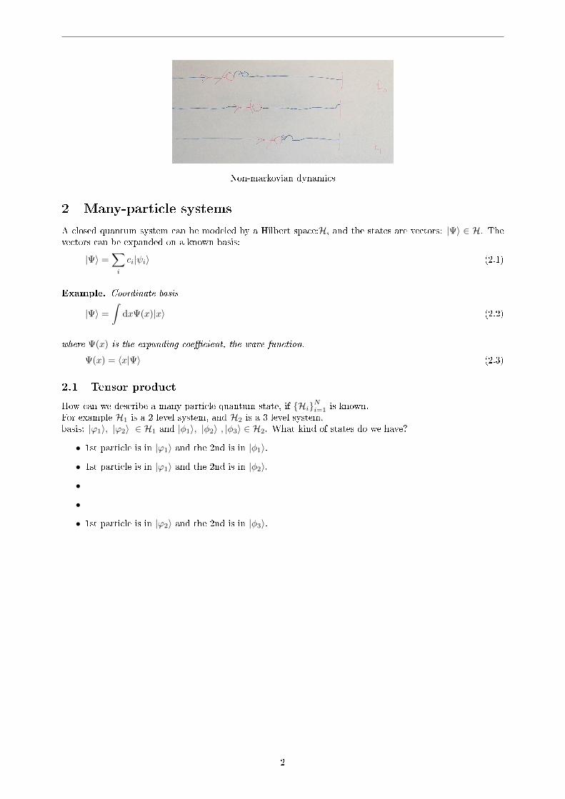
Non-markovian dynamics

2 Many-particle systems

A closed quantum system can be modeled by a Hilbert space:H, and the states are vectors: |Ψ〉 ∈ H. Thevectors can be expanded on a known basis:

|Ψ〉 =∑i

ci|ψi〉 (2.1)

Example. Coordinate basis

|Ψ〉 =

∫dxΨ(x)|x〉 (2.2)

where Ψ(x) is the expanding coecient, the wave function.

Ψ(x) = 〈x|Ψ〉 (2.3)

2.1 Tensor product

How can we describe a many particle quantum state, if HiNi=1 is known.For example H1 is a 2 level system, and H2 is a 3 level system.basis: |ϕ1〉, |ϕ2〉 ∈ H1 and |φ1〉, |φ2〉 , |φ3〉 ∈ H2. What kind of states do we have?

• 1st particle is in |ϕ1〉 and the 2nd is in |φ1〉.

• 1st particle is in |ϕ1〉 and the 2nd is in |φ2〉.

•

•

• 1st particle is in |ϕ2〉 and the 2nd is in |φ3〉.

2

2.2 Inner product of tensor product vectors

The mathematical notation for this is

|Φ11〉 = |ϕ1〉 ⊗ |φ1〉 −→

100000

=

(10

)⊗

100

|Φ12〉 = |ϕ1〉 ⊗ |φ1〉 −→

010000

=

(10

)⊗

010

...

|Φ23〉 = |ϕ2〉 ⊗ |φ3〉 −→

000001

=

(01

)⊗

001

,

(2.4)

and in general

(ab

)⊗

αβγ

=

aαaβaγbαbβbγ

(2.5)

In arbitrary dimension: |Φij〉 = |ϕi〉 ⊗ |φj〉 ≡ |ϕi〉|φj〉. This is the tensor product of the two vectors.Notion for the tensor product of Hilbert spaces: H1 ⊗H2

Remark. Dimension of the product space:

dim(H1 ⊗H2) = dim(H1)dim(H2) (2.6)

Remark. The ⊗ sign also denotes the direct product of two groups, which is the Cartesian product ofgroups. For abelian groups, like vector spaces it is called direct sum, and denoted by ⊕, and dim(V1⊕V2) =dim(V1) + dim(V2) An easy example for direct sum in quantum mechanics is when we have a tight bindingmodel with n sites, than the dimension of one particle in this system is n. If we add m more sites, than thedimension of the system will be n+m.

2.2 Inner product of tensor product vectors(〈ϕ′|〈φ′|

)(|ϕ〉|φ〉

)= 〈ϕ′|ϕ〉〈φ′|φ〉 (2.7)

Partial inner product.

〈ϕ′(1)|(|ϕ〉|φ〉

)= 〈ϕ′|ϕ〉|φ〉

〈φ′(2)|(|ϕ〉|φ〉

)= |ϕ〉〈φ′|φ〉

(2.8)

The upper index (1),(2) shows us that on which vector acts the inner product.

2.3 Tensor product of operators

(A⊗B)(|ϕ〉 ⊗ |φ〉) = A|ϕ〉 ⊗B|φ〉 (2.9)

3

2.4 Density operator

If the operator acts on only the rst Hilbert space, than it is A ⊗ 11(2), and if it acts only on the second,than 11(1) ⊗A. Also we can write A(1) and A(2).

2.4 Density operator

A closed quantum system can be described by its state vector |Ψ〉, and usually we are interested in operatorexpected values.

〈A〉 = 〈Ψ|A|Ψ〉 ≡ Tr(ρA), (2.10)

where ρ = |Ψ〉〈Ψ| is the density operator of a pure state.Now assume that our total system consist of a smaller subsystem and a bath. We are only interested in

the subsystem. The state of the total system is

|Ψ〉 =∑ia

cia|ϕi〉|φa〉, (2.11)

and we want to calculate 〈A〉, where A act only on the subsystem.

〈A〉 = 〈Ψ|A⊗ 11B|Ψ〉 =∑ia

∑jb

c∗jbcia〈ϕj |A|ϕi〉 〈φb|φa〉︸ ︷︷ ︸δab

=∑ij

(∑a

c∗jacia

)〈ϕj |A|ϕi〉 (2.12)

Introducing the reduced density operator:

(ρS)ij =∑a

ciac∗ja, (2.13)

which is also

ρS = TrB(|Ψ〉〈Ψ|) = TrB(ρT). (2.14)

TrB denotes the partial trace which means TrB(ρ) =∑a〈φ

(B)a |ρ|φ(B)

a 〉 With this denition

〈A〉 = TrS(ρSA). (2.15)

Usually we can't calculate ρS from |Ψ〉, but if the system is at the state ψα with probability pα, than

ρS =∑α

pα|ψα〉〈ψα| (2.16)

|ψα is not necessarly orthogonal. The decomposition of |ψα〉 from ρS is not unique.

Remark. The density operator is like a generalization of the probability. For example if two random variableis independent, than their joint distribution is the product of the two distribution. i.e.

pij = p(1)i p

(2)j . (2.17)

For density operators it is tensor product, i.e.

ρT = ρ1 ⊗ ρ2. (2.18)

And for general pij the marginal probability distribution is

p(1)i =

∑j

pij , (2.19)

which is for density operator is the partial trace

ρ1 = Tr2(ρ) =∑j

〈φ(2)j |ρ|φ(2)j 〉 (2.20)

and the diagonal elements of this expression is exactly the marginal distribution.

4

2.5 Properties of the density operator

2.5 Properties of the density operator

• ρ is hermitian.

• Tr(ρ) = 1

• Tr(ρ2) ≤ 1 and equal 1 only if ρ is pure.

• positive semidenite

3 Redeld equation

Original paper: Redeld - On the theory of relaxation processes. [1]Projection Operator Techniques: Nakajima-Zwanzig equation [2, 3]Recommended literature: Breuer, Petruccione - The Theory of Open Quantum System[4]. Contains boththe derivations.

HT = HS +HB +HSB (3.1)

where HT is the total, HS is the system, HB is the bath Hamiltonian and HSB is the coupling between themwhich is assumed to be small.

HSB =∑α

Aα ⊗Bα (3.2)

where Aα and Bα are both hermitian. First let's examine the equilibrium state of the system. At inversetemperature β if we assume Boltzmann distribution than the whole density operator is

ρ(equilibrium)T =

e−βHT

ZT(3.3)

If there is no interaction between the system of interest and the bath, i.e. HSB = 0, than

ρ(eq)

S

∣∣∣HSB=0

≡ TrBρ(eq)

T

∣∣∣HSB=0

=e−βHS

ZS, (3.4)

because the system and the bath Hamiltonian commute. If there is interaction between the system and thebath, than the system distribution is not the Boltzmann distribution. Usually the interaction is only at thesurface of the system, which is small compared to the volume, so the interaction is very small which causesthat the Boltzmann distribution is approximately correct.

The dynamics of the total system is described by the von Neumann equation.

ρ(t) = −i [H, ρ(t)] (3.5)

Interaction picture: XI(t) = eiH0tX(t)e−iH0t, where H0 = HS +HB.

ρI(t) = −i[HI

SB(t), ρI(t)]

(3.6)

Solving it formally, than iteratively up to second order in the magnitude of HSB:

ρI(t) = ρ(0)− i∫ t

0

dt′[HI

SB(t′), ρI(t′)]

= ρ(0)− i∫ t

0

dt′[HI

SB(t′), ρI(0)]−∫ t

0

dt′∫ t′

0

dt′′[HI

SB(t′),[HI

SB(t′′)]ρI(t′′)

] (3.7)

Substituting t′′ 7→ t′ − t′′.

ρI(t) = ρ(0)− i∫ t

0

dt′[HI

SB(t′), ρI(0)]−∫ t

0

dt′∫ t′

0

dt′′[HI

SB(t′),[HI

SB(t′ − t′′)]ρI(t′ − t′′)

](3.8)

5

Writing again in integro-dierential equation form we obtain the Redeld equation.

ρI(t) = −i[HI

SB(t′), ρI(0)]−∫ t

0

dt′[HI

SB(t),[HI

SB(t− t′)]ρI(t− t′)

](3.9)

So far there was no approximation, but we are interested only in system variables. Now we perform the so-called Born approximation which says that the bath is much larger than the system so if it was at Boltzmanndistribution at the beginning, than it will remain in it, and the density operator can be written in productform. Formally ρ(t) ≈ ρS(t)⊗ ρB, where ρB is time independent. Now we trace over bath variables.

ρIS(t) = −iTrB[HI

SB(t′), ρS(0)⊗ ρB]−∫ t

0

dt′TrB[HI

SB(t),[HI

SB(t− t′)]ρIS(t− t′)⊗ ρB

](3.10)

1 This is a closed integro-dierential equation for ρS, but it has many disadvantages. The diagonal elementsof ρS are probabilities, so they must be non-negative, and we assume that they converge to the Boltzmanndistribution. Unfortunately this equation doesn't fulll these conditions. There are methods which tries tosolve this problem e.g. the initial slippage condition [5], or the polaron transformation [6, 7]. First term onthe right hand side: TrB(BαρB) = 0. Than we expand HI

SB

ρIS(t) = −∑αβ

∫ t

0

dt′AIα(t)AI

β(t− t′)ρIS(t− t′)TrB(BIα(t)BI

β(t− t′)ρB)

−AIα(t)ρIS(t− t′)AI

β(t− t′)TrB(BIα(t)ρBB

Iβ(t− t′)

)−AI

β(t− t′)ρIS(t− t′)AIα(t)TrB

(BIβ(t− t′)ρBBI

α(t))

ρIS(t− t′)AIβ(t− t′)AI

α(t)TrB(ρBB

Iβ(t− t′)BI

α(t))

(3.11)

The rst two terms are the hermitian conjugate of the second two terms. In the TrB the bath correlationfunction appears. E.g.

TrB(BIα(t)BI

α(t− t′)ρB)

= TrB

(eiHBtBαe

−iHBteiHB(t−t′)BβeiHB(t−t′) e

βHB

ZB

)= TrB

(eiHBt

′Bαe

−iHBt′Bβ

eβHB

ZB

)= TrB

(BIα(t′)Bβ

eβHB

ZB

)= 〈BI

α(t′)Bβ〉B ≡ Cαβ(t′)

(3.12)

Cαβ(t) is the correlation function.

Proposition. Cαβ(−t) = C∗βα(t)

Proof. trivial

Equation (3.11) is a non-markovian equation. It depend on the whole history of ρIS(t). But if the bathcorrelation function decays fast enough e.g. C(t) ∼ exp(−t/τB) with large τB, than ρIS(t − t′) 7→ ρIS(t)substitution is valid in the integral, and the upper limit of the integral might goes to innity.

ρIS(t) = −∑αβ

∫ ∞0

dt′AIα(t)AI

β(t− t′)ρIS(t)Cαβ(t′)−AIα(t)ρIS(t)AI

β(t− t′)C∗αβ(t′)

−AIβ(t− t′)ρIS(t)AI

α(t)Cαβ(t′) + ρIS(t)AIβ(t− t′)AI

α(t)C∗αβ(t′)

(3.13)

The rst term is the hermitian conjugate of the last, and same with the second and third. Now we haveonly system operators, and we can write them back to Schrödinger picture, which means we multiply with

1In the Breuer, Petruccione book[4], in the "Projection operator techniques" chapter there is a long derivation, whichshows how to go beyond the Born approximation. There are two methods for it, the Nakajima-Zwanzig equation and thetime-convolutionless projection operator technique.

6

3.1 Secular Approximation

exp(−iHSt) from left, and with exp(iHSt) from right. operators. E.g.

e−iHStAIα(t)ρIS(t)AI

β(t− t′)eiHSt =

e−iHSt(eiHStAαe

−iHSt) (eiHStρS(t)e−iHSt

) (eiHS(t−t′)Aβe

−iHS(t−t′))eiHSt =

AαρS(t)AIβ(−t′)

(3.14)

The Redeld equation in Schrödinger picture:

ρS(t) + [HS, ρS(t)] = −∑αβ

∫ ∞0

dt′(AαA

Iβ(−t′)ρS(t)Cαβ(t′)−AαρIS(t)AI

β(−t′)C∗αβ(t′))

+ h.c. (3.15)

Introducing the Tα =∑β

∫∞0

dtCαβ(t)AIβ(−t)

ρS(t) + i [HS, ρS(t)] =∑α

(AαρS(t)T †α −AαTαρS(t) + h.c.

)(3.16)

If Cαβ(t) decays very fast, i.e. Cαβ(t) = Γαβδ(t), than Tα =∑β ΓαβAβ . This is the same result as in the

singular-coupling limit (section 5). But in general expanding Tα on energy basis:

(Tα)ij =∑β

∫ ∞0

Cαβ(t)ei(εj−εi)t(Aβ)ij =∑β

Γαβ(ωji)(Aβ)ij , (3.17)

where ωji = εj − εi, and Γαβ(ω) =∫∞0

dtCαβ(t)eiωt

3.1 Secular Approximation

Tα =∑ij

(Tα)ij |i〉〈j| =∑β

∑ω

Γαβ(ω)∑ij

(Aβ)ijδω,ωji |i〉〈j| =∑β

∑ω

Γαβ(ω)Aβ(ω), (3.18)

where Aβ(ω) =∑ij(Aβ)ij |i〉〈j|δω,ωji , so

∑ω Aβ(ω) = Aβ .

Proposition. A†α(ω) = Aα(−ω)

The Redeld equation with these quantities:

ρS + i [HS, ρS] =∑α

(AαρST

†α + TαρSA

†α −A†αTαρS − ρST †αAα

)=∑αβ

∑ωω′

(Aα(ω′)ρSΓ∗αβ(ω)A†β(ω) + Γαβ(ω)Aβ(ω)ρSA

†α(ω′)

−A†α(ω′)Γαβ(ω)Aβ(ω)ρS − ρSΓ∗αβ(ω)A†β(ω)Aα(ω′)) (3.19)

If we had worked in interaction picture, our equation would look like

ρIS =∑αβ

∑ωω′

(ei(ω−ω

′)tAα(ω′)ρISΓ∗αβ(ω)A†β(ω) + e−i(ω−ω′)tΓαβ(ω)Aβ(ω)ρISA

†α(ω′)

− e−i(ω−ω′)tA†α(ω′)Γαβ(ω)Aβ(ω)ρIS − ei(ω−ω

′)tρISΓ∗αβ(ω)A†β(ω)Aα(ω′)).

(3.20)

A useful identity to derive this is AI(ω) = e−iωtA(ω). If exp((ω − ω′)t) is fast compared to the intrinsicevolution of the system, than only the nonsecular terms (ω − ω′ 6= 0) are neglectable. This is a goodapproximation e.g. in quantum optics.

ρIS =∑αβ

∑ω

(Aα(ω)ρISΓ∗αβ(ω)A†β(ω) + Γαβ(ω)Aβ(ω)ρISA

†α(ω)

−A†α(ω)Γαβ(ω)Aβ(ω)ρIS − ρISΓ∗αβ(ω)A†β(ω)Aα(ω)).

(3.21)

7

3.2 Lindblad form

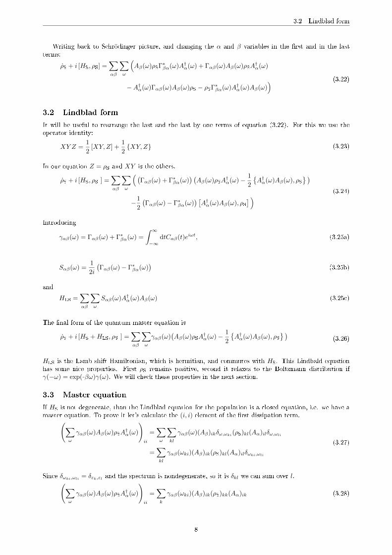
Writing back to Schrödinger picture, and changing the α and β variables in the rst and in the lastterms:

ρS + i [HS, ρS] =∑αβ

∑ω

(Aβ(ω)ρSΓ∗βα(ω)A†α(ω) + Γαβ(ω)Aβ(ω)ρSA

†α(ω)

−A†α(ω)Γαβ(ω)Aβ(ω)ρS − ρSΓ∗βα(ω)A†α(ω)Aβ(ω)) (3.22)

3.2 Lindblad form

It will be useful to rearrange the last and the last by one terms of equation (3.22). For this we use theoperator identity:

XY Z =1

2[XY,Z] +

1

2XY,Z (3.23)

In our equation Z = ρS and XY is the others.

ρS + i [HS, ρS ] =∑αβ

∑ω

( (Γαβ(ω) + Γ∗βα(ω)

) (Aβ(ω)ρSA

†α(ω)− 1

2

A†α(ω)Aβ(ω), ρS

)−1

2

(Γαβ(ω)− Γ∗βα(ω)

) [A†α(ω)Aβ(ω), ρS

] ) (3.24)

Introducing

γαβ(ω) = Γαβ(ω) + Γ∗βα(ω) =

∫ ∞−∞

dtCαβ(t)eiωt, (3.25a)

Sαβ(ω) =1

2i

(Γαβ(ω)− Γ∗βα(ω)

)(3.25b)

and

HLS =∑αβ

∑ω

Sαβ(ω)A†α(ω)Aβ(ω) (3.25c)

The nal form of the quantum master equation is

ρS + i [HS +HLS, ρS ] =∑αβ

∑ω

γαβ(ω)(Aβ(ω)ρSA

†α(ω)− 1

2

A†α(ω)Aβ(ω), ρS

)(3.26)

HLS is the Lamb shift Hamiltonian, which is hermitian, and commutes with HS. This Lindbald equationhas some nice properties. First ρS remains positive, second it relaxes to the Boltzmann distribution ifγ(−ω) = exp(−βω)γ(ω). We will check these properties in the next section.

3.3 Master equation

If HS is not degenerate, than the Lindblad equation for the population is a closed equation, i.e. we have amaster equation. To prove it let's calculate the (i, i) element of the rst dissipation term.(∑

ω

γαβ(ω)Aβ(ω)ρSA†α(ω)

)ii

=∑ω

∑kl

γαβ(ω)(Aβ)ikδω,ωki(ρS)kl(Aα)ilδω,ωli

=∑kl

γαβ(ωki)(Aβ)ik(ρS)kl(Aα)ilδωki,ωli

(3.27)

Since δωki,ωli = δεk,εl and the spectrum is nondegenerate, so it is δkl we can sum over l.(∑ω

γαβ(ω)Aβ(ω)ρSA†α(ω)

)ii

=∑k

γαβ(ωki)(Aβ)ik(ρS)kk(Aα)ik (3.28)

8

We can see, that it only depend on the diagonal terms of ρS. For the anti-commutator term the same istrue. In the master equation the von Neumann term has no contribution, not even the Lamb shift term,because it commutes with the system Hamiltonian. The nal form is

Pi =∑j

WijPj −∑j

WjiPi, (3.29)

where

Pi = (ρS)ii (3.30a)

and

Wij =∑αβ

γαβ(εj − εi)(Aα)ji(Aβ)ij (3.30b)

The system converges to the Boltzmann distribution if Wji = exp(−β(εj − εi))Wij .

4 Bath correlation function and spectral density

So far we didn't speak about the correlation function (Cαβ(t)) and its Fourier transformation (γαβ(ω)). Wecan calculate them from scratch. There are two popular systems for bath. The rst is the bath of photons.This is often used in quantum optics. The second is the bath of phonons, which is used in solid state physics.Both can be traced back to the harmonic oscillator, so we start with that.

4.1 Harmonic oscillator correlation function

The Hamiltonian of the harmonic oscillator is

Hosc =p2

2m+mω

2x2 = ~

(a†a+

1

2

), (4.1)

where

a =

√mω

2~

(x+

i

mωp

)a† =

√mω

2~

(x− i

mωp

) (4.2)

are the ladder operators, satisfying the [a, a†] = 1 relation. We can express x with theese operators.

x =

√~

2mω(a† + a) (4.3)

The ladder operators in Heisenber picture are 2

a(t) = eiHosct/~ae−iHosct/~ = ae−iωt

a†(t) = eiHosct/~a†e−iHosct/~ = a†eiωt.(4.4)

The correlaction function by denition is

C(t) := 〈x(t)x〉, (4.5)

where the average means termical average i.e. 〈x(t)x〉 ≡ Z−1Tr(exp (−βHosc)x(t)x).

C(t) =~

2mω〈(a†(t) + a(t))(a† + a)〉 =

~2mω

(〈a†a〉eiωt + 〈aa†〉e−iωt) (4.6)

2If A is an operator in Schrödinger picture, than the notion for Heisenberg picture will be A(t), since use here only timeindependent operators.

9

4.2 Interaction with phonons

The 〈aa〉 and 〈a†a†〉 term is zero. The remaining two quantity is the occupation number i.e.

〈a†a〉 ≡ n =1

eβ~ω − 1

〈aa†〉 = 〈a†a〉+ 1

(4.7)

Substituting this back to the correlation function

C(t) =~

2mω

(〈a†a〉eiωt + (〈a†a〉+ 1)e−iωt

)=

~2mω

(2〈a†a〉 cos(ωt) + cos(−ωt) + i sin(−ωt)

)=

~2mω

(cos(ωt)

(1 +

2

eβ~ω − 1

)− i sin(ωt)

)=

~2mω

(coth

(β~ω

2

)cos(ωt)− i sin(ωt)

)(4.8)

4.2 Interaction with phonons

Assume our system is an electron which moves in a solid. The solid consist of ions which are in a lattice,but they can vibrate around their equilibrium point. This is called lattice vibration and the eigenmodes arethe phonons. In second quantized form it is [8]

Hion =∑q,λ

~ωλ(q)a†λ(q)aλ(q) (4.9)

If an electron moves in solid, than it interacts with the ions [9]. The Hamilon operator for this term is (incoordinate representation)

Hel-ion(ri; Rl) =∑i

Uel-ion(ri; Rl), (4.10)

where ri is the position of the ith electron, and Rl is the position of the lth ion, and Uel-ion(ri; Rl) is justthe Coulomb interaction between the ith electron and the ions. If the displacement of the ions are small,than Rl ≈ R0

l + ul, and

Hel-ion(ri; Rl) =∑i

∑l

∂Uel-ion(ri; Rl)∂u(R0

l )

∣∣∣u(R0

l )=0u(R0

l ) (4.11)

The rst factor at the right hand side is the function of the electrons and the second is only the iondisplacements. This u(R0

l ) correspondes to the x in the harmonic oscillator. The proper way to expand itwith phonon creation and annihilation operators is

u(R0l ) =

∑q,λ

√~

2MNωλ(q)e(λ)(q)e−qR

0l (aλ(q) + a†λ(−q)) (4.12)

For more detail check Jen® Sólyom - Fundamentals of the Physics of Solids, Volume II: Electron proberties,Chapter 23: Electrons in Thermally Vibrating Lattices [9].

4.3 Interaction with photons

Assume we have an atom or molecule, which interacts with the quantized radiation eld. The operator forthe photons is

Hphoton =∑

q,λ=1,2

~ω(q)a†λ(q)aλ(q). (4.13)

In the dipole approximation the interaction term is

Hph-dip = −DE, (4.14)

10

4.4 Spectral density

where E is the electric eld, and D is the dipole momentum of the molecula. It can also be expressed withladder operators:

E = i∑

q,λ=1,2

√2π~ω(q)

Veλ(q)

(aλ(q)− a†λ(q)

)(4.15)

In this setup E correspondes to the x in the harmonic oscillator.

4.4 Spectral density

We've seen, that both in the phonon and the photon case the bath operator has the form

B =∑µ

cµxµ =∑µ

gµ(aµ + a†µ), (4.16)

where µ is equivalent to q and λ. The correlation function is

〈B(t)B〉 =∑µν

cµcν〈xµ(t)xν〉 (4.17)

If xµ and xν are independent, than

〈B(t)B〉 =∑µ

cµcµ〈xµ(t)xµ〉

=∑µ

gµgµ

(coth(

β~ωµ2

) cos(ωµt)− i sin(ωµt)

)

=~π

∫ ∞0

dωJ(ω)

(coth(

β~ω2

) cos(ωt)− i sin(ωt)

),

(4.18)

where formally

J(ω) = π∑µ

g2µδ(ω − ωµ) (4.19)

is the spectral density. We will not calculate here the exact for of J(ω), only same hand-waving countingfor the dominant ω dependence.In general gµ ∼ ω(|q|)α/2, where α = −1 for phonons and α = 1 for photons.We assume that both the dispersion relations are linear in q. The summation over µ is in our models arethe summation over q, so∑

µ

g2µ(. . . )→∑q

ωα(q)(. . . ) ∼∫

d3qωα(q)(. . . )

∼∫

dΩ

∫dqq2ωα(q)(. . . ) ∼

∫dΩ

∫dωω2ωα(. . . )

(4.20)

We see that for phonons J(ω) ∼ ω and for photons J(ω) ∼ ω3

Remark. In our examples there were more bath operators. E had three components, and in the phononcase besided that there is an u(R0

l ) in every lattice site. But they are independent as long as we consider

quadratic bath Hamiltonians (4.9) (4.13) For example with phonons: [aλ(q), a†λ′(q′)] = δλλ′δqq′ , so

〈ui(R0l ; t)uj(R

0l′)〉 = 〈ui(R0

l ; t)ui(R0l )〉δll′δij (4.21)

4.5 Correlation function Fourier transform

In the Lindblad equation we are only interested in the Fourier transform of the correlation function.

γ(ω) =

∫ ∞−∞

dteiωtC(t) (4.22)

11

Substituting equation (4.18) into C(t) yields

γ(ω) =

∫ ∞−∞

dteiωt~π

∫ ∞0

dω′J(ω′)

(coth(

β~ω′

2) cos(ω′t)− i sin(ω′t)

)=

~π

∫ ∞0

dω′J(ω′)

∫ ∞−∞

dteiωt(

coth(β~ω′

2) cos(ω′t)− i sin(ω′t)

),

(4.23)

In the second integral the sin and cos functions can be expressed with eponential function, then the inte-gration over t can be evaluated, and we get Dirac deltas.

γ(ω) =~π

∫ ∞0

dω′J(ω′)

(coth(

β~ω′

2)(δ(ω + ω′) + δ(ω − ω′)

)− δ(ω + ω′) + δ(ω − ω′)

)

=

J(−ω)(coth(β~ω2 )− 1) = −J(−ω)

2

1− e−β~ω| ω < 0

J(ω)(coth(β~ω2 ) + 1) = J(ω)2

1− e−β~ω| ω > 0

(4.24)

For phonon bath the nal form is

γ(ω) = ηωe−|ω|ωc

1

1− e−β~ω, (4.25)

where ωc is the cuto frequency, and this is the consequence of working in a nite lattice. The η quantitymight be also depends on ωc.For photon bath

γ(ω) =4ω3

3~c31

1− e−β~ω, (4.26)

Both of these function satisfyes the detailed balance condition i.e.

γ(−ω) = e−β~ωγ(ω) (4.27)

Remark. In the literature J(ω) ∼ ω is called Ohmic spectral density. For J(ω) ∼ ωκ κ < 1 is the sub-Ohmic, and κ > 1 is the super-Ohmic spectral density.

If we want to satifsy the detailed balance condition, than J(ω) must be an odd function.

5 Singular-coupling limit

In the singular-coupling limit one assumes that the interaction between the system and the bath is verystrong. Formally the total Hamiltonian is

HT = HS + ε−2HB + ε−1HSB (5.1)

and we want to derive a closed equation for ρS in the limit of ε → 0. After a similar derivation [10] to theweak-coupling limit the nal equation is

d

dtρS + i[HS +HLS, ρS] =

∑αβ

γαβ

(AβρSAα −

1

2AαAβ , ρS

), (5.2)

where γαβ = γαβ(ω = 0) and Sαβ = Sαβ(ω = 0). In that case the equilibrium distribution is always theuniform distribution.

6 Fermi's Golden rule

In quantum mechanics lecture we have derived the Fermi's Golden rule.

ρnm =∑m

Wnmρmm −∑n

Wmnρnn, (6.1)

12

REFERENCES

where

Wnm = 2π|(H ′)nm|2δ(En − Em). (6.2)

Now ρ is the total density operator, H ′ is the system-bath interaction (HSB), and a state consist of thesystem and the bath state, i.e. |n〉 = |i〉|a〉. The full energy of the unperturbed system is En ≡ Eia = εi+E

Ba ,

where EBa is the energy of the bath.

The equation for the populations of the total system is

(ρT)ia,ia =∑jb

Wia,jb(ρT)jb,jb −∑jb

Wjb,ia(ρT)ia,ia. (6.3)

As before, we are only interested in the dynamics of the system, and we perform the Born approximation:(ρT)ia,jb = (ρS)ij(ρB)ab, where we assume, that the bath is in termal equilibrium: (ρB)ab ∼ exp (−βEB

a )δabSumming over the bath variables in 6.3 yields the equation of motion of the system.

(ρS)ii =∑j

∑ab

Wia,jb(ρB)bb︸ ︷︷ ︸Wij

(ρS)jj −∑j

∑ab

Wjb,ia(ρB)aa︸ ︷︷ ︸Wji

(ρS)ii (6.4)

We are interested in this new Wij quantity. First rewrite the denition of Wnm (equation 6.2) with (ia)indeces, and expanding the Dirac delta with exponential functions.

Wia,jb =

∫ ∞−∞

dt|〈i a|HSB|j b〉|2e−i((εi+EB

a )−(εj+EB

b ))t

=

∫ ∞−∞

dt〈i a|HSB|j b〉〈j b|HSB|i a〉e−i((εi+EB

a )−(εj+EB

b ))t

=∑αβ

∫ ∞−∞

dt(Aβ)ij(Aα)jiei(εj−εi)t(Bβ)ab e

iEB

b t(Bα)bae−iEB

a t︸ ︷︷ ︸(BIα(t))ba

(6.5)

We multiply this equation with (ρB)bb and sum over a and b to obtain Wij .

Wij =∑αβ

∫ ∞−∞

dt(Aβ)ij(Aα)jiei(εj−εi)t

∑ab

(ρB)bb(BIα(t))ba(Bβ)ab (6.6)

The hinder part of the right-hand side is the bath correlation function∑ab

(ρB)bb(BIα(t))ba(Bβ)ab = TrB(ρBB

Iα(t)Bβ) = 〈BI

α(t)Bβ〉B = Cαβ(t) (6.7)

Putting it back to the equation of Wij .

Wij =∑αβ

∫ ∞−∞

dt(Aβ)ij(Aα)jiei(εj−εi)tCαβ(t) =

∑αβ

(Aβ)ij(Aα)jiγαβ(εj − εi) (6.8)

Which is the same as equtaion (3.30b).

References

[1] A. Redeld, On the Theory of Relaxation Processes, IBM J. Res. Dev., januar 1957.

[2] S. Nakajima, On Quantum Theory of Transport Phenomena (in German), Progress of TheoreticalPhysics, 1958.

[3] R. Zwanzig, Ensemble Method in the Theory of Irreversibility (in German), Journal of ChemicalPhysics, 1960.

[4] H.-P. Breuer and F. Petruccione, The Theory of Open Quantum Systems. 01 2006.

13

REFERENCES

[5] P. Gaspard and M. Nagaoka, Slippage of initial conditions for the Redeld master equation, TheJournal of Chemical Physics, vol. 111, no. 13, pp. 56685675, 1999.

[6] D. Xu and J. Cao, Non-canonical distribution and non-equilibrium transport beyond weak system-bathcoupling regime: A polaron transformation approach, Frontiers of Physics, vol. 11, p. 110308, May2016.

[7] C. K. Lee, J. Moix, and J. Cao, Coherent quantum transport in disordered systems: A unied polarontreatment of hopping and band-like transport, The Journal of Chemical Physics, vol. 142, no. 16,p. 164103, 2015.

[8] J. Sólyom, Fundamentals of the Physics of Solids, Volume II: Electron properties. Springer.

[9] J. Sólyom, Fundamentals of the Physics of Solids, Volume I: Fundamental of the Physics of Solids.Springer.

[10] A. Rivas and S. Huelga, Open Quantum Systems: An Introduction. Springer, 2011.

14