Nondestructive Characterization of Soft Materials and ...

Nondestructive Characterization of Soft Materials and Biofilms by Measurement of Guided Elastic Wave

Propagation Using Optical Coherence Elastography

Journal: Soft Matter

Manuscript ID SM-ART-09-2018-001902.R1

Article Type: Paper

Date Submitted by the Author: 23-Nov-2018

Complete List of Authors: Liou, Hong-Cin; Northwestern University, Mechanical Engineering DepartmentSabba, Fabrizio; Northwestern University, Civil and Environmental Engineering DepartmentPackman, Aaron; Northwestern University, Civil and Environmental Engineering DepartmentWells, George; Northwestern University, Civil and Environmental Engineering DepartmentBalogun, Oluwaseyi; Northwestern University, Mechanical Engineering Department; Northwestern University, Civil and Environmental Engineering Department

Soft Matter

1 Nondestructive Characterization of Soft Materials and Biofilms by

2 Measurement of Guided Elastic Wave Propagation Using Optical Coherence

3 Elastography

4

5

6 Hong-Cin Liou1, Fabrizio Sabba2, Aaron Packman2, George Wells2, Oluwaseyi Balogun1,2*

7

8

9 1Mechanical Engineering Department, Northwestern University, Evanston, IL 60208

10 2Civil and Environmental Engineering Department, Northwestern University, Evanston, IL

11 60208

12

13

14 *Corresponding author

15 [email protected]

16 +1-847-491-3054

17

18

19

20

Page 1 of 36 Soft Matter

2

21 ABSTRACT

22

23 Biofilms are soft multicomponent biological materials composed of microbial communities attached to

24 surfaces. Despite the crucial relevance of biofilms to diverse industrial, medical, and environmental

25 applications, biofilm mechanical properties are understudied. Moreover, most available techniques for

26 characterization of biofilm mechanical properties are destructive. Here, we detail a model-based approach

27 developed to characterize the viscoelastic properties of soft materials and bacterial biofilms based on

28 experimental data obtained with the nondestructive dynamic optical coherence elastography (OCE)

29 technique. The model predicted the frequency- and geometry-dependent propagation velocities of elastic

30 waves in a soft viscoelastic plate supported by a rigid substratum. Our numerical calculations suggest that

31 the dispersion curves of elastic waves recorded in thin soft plates by the dynamic OCE technique was

32 dominated by guided waves, whose phase velocities strongly depended on the viscoelastic properties and

33 the plate thicknesses. The numerical model was validated against experimental measurements in agarose

34 phantom samples with different thicknesses and concentrations. The model was then used to interpret

35 guided wave dispersion curves obtained by OCE technique in bacterial biofilms developed in a rotating

36 annular reactor, which allowed for a quantitative characterization of biofilm shear modulus and viscosity.

37 This study is the first to employ measurements of elastic wave propagation to characterize biofilms, and

38 provides a novel framework combining a theoretical model and experimental approach for studying the

39 relationship between biofilm internal physical structure and mechanical properties.

40

41 Keywords: nondestructive optoacoustic imaging, optical coherence elastography, viscoelastic properties,

42 guided elastic wave propagation, biofilms

43

44

Page 2 of 36Soft Matter

3

45 1. Introduction

46

47 Biofilms are multicomponent biological materials composed of communities of microorganisms attached

48 to a surface and encased in a self-produced matrix of extracellular polymeric substances (EPS)1, 2. Biofilms

49 are the dominant mode of microbial life in aquatic systems, soil and sediment, and play a critical role in

50 biogeochemical cycling, food webs, and symbioses3-6. The mechanical properties of biofilms have recently

51 attracted substantial attention from researchers but remain understudied7-9. It has been shown that biofilms

52 display properties of both elastic solids and viscous liquids in response to stress, and can thus be viewed as

53 viscoelastic biomaterials analogous to soft biological tissues8, 10-12. Biofilm mechanical properties depend

54 on morphology and composition, and are thought to influence important processes like detachment,

55 attachment, and mass transfer characteristics that are crucial to biofilm functions13, 14. Recent macro-scale

56 quasi-static experiments on biofilm mechanical properties suggest that (1) biofilm mechanical properties

57 are heterogeneous8, 15; (2) viscoelastic behavior occurs at small deformations16, 17; (3) viscoplastic behavior

58 occurs at large deformations when the internal stresses are relieved10, 15, 18, 19; and (4) biofilms are stiffer

59 near the attachment surface and more flexible in their canopy20. The latter suggests biofilm mechanical

60 properties can vary with distance from the attachment surface.

61 Most work to date on biofilm mechanical properties has employed macro- and micro-rheological

62 techniques to measure mechanical properties. These techniques have some limitations: macro-rheological

63 techniques only measure bulk average of the properties and do not reveal spatial variability and complexity

64 of living biofilms21-23, whereas micro-rheological techniques yield only highly localized measurements,

65 often on biofilms ex situ, and are not capable of spatial mapping at the mm to cm scale24-28. Additionally,

66 these techniques require sample disruption or structural changes while testing. Recently, elastography

67 techniques have enabled biomechanical characterization of soft structures, particularly in the biomedical

68 engineering community, by combining diagnostic imaging tools with specimen deformation approaches. In

69 these techniques, the spatial deformation of a biological specimen is mapped under an applied external

70 force, allowing for identification of mechanical contrast regions and stiff tissues associated with different


4

71 disease states. Among existing elastography techniques including magnetic resonance elastography

72 (MRE)29, ultrasound elastography (USE)30, 31, and optical coherence elastography (OCE)32-34, the OCE

73 technique provides superior characteristics such as (1) micron-scale spatial resolution, (2) high sample

74 displacement sensitivity on the nanometer scale, and (3) high temporal resolution and fast image acquisition

75 time. These features facilitate the detection of small sample deformations and provide the potential to track

76 dynamic mechanical deformations in real time. OCE techniques can be classified as static or dynamic

77 methods, depending on the time scale of the specimen deformation. Static OCE methods have been widely

78 applied in biomechanical characterization experiments in the biomedical research community, where the

79 heterogeneous strain map of tissue specimens produced in response to a uniform stress field is used to

80 predict the local Young’s modulus. This modulus is based on the ratio of the stress and strain, as obtained

81 in a linear elastic solid. Measurements of viscoelastic properties, on the other hand, rely on tracking

82 temporal dynamics of the specimen deformation under the applied stress field. This is achieved using

83 dynamic OCE methods, in which creep relaxation dynamics35, elastic stress wave propagation36-41, or

84 underdamped acoustic vibrations42, 43 are recorded using various motion tracking methods. These methods

85 can be classified into speckle tracking methods and phase sensitive optical coherence tomography (OCT).

86 The latter is of great interest because it provides a larger measurement dynamic range and inexpensive

87 options for data acquisition38.

88 This paper provides the first-of-its-kind OCE characterization of viscoelastic properties in bacterial

89 biofilms based on elastic stress wave propagation measurements. Elastic wave based dynamic OCE

90 methods have been explored exclusively in biomedical applications for characterization of viscoelastic

91 properties in soft tissues36, 37, 44; however, biofilms have more complex geometrical and compositional

92 features. These features, including heterogeneous composition, surface roughness, non-uniform porosity

93 distribution, and bacterial hierarchical stratification11, 19, 45-47, make modeling of elastic waves in these

94 materials challenging and invaluable for interpreting the experimental data. In this paper, we report a

95 layered theoretical model that predicted the velocities of guided elastic waves at different frequencies in a

96 soft viscoelastic plate with various thicknesses, shear moduli, and complex shear viscosities. The layered


5

97 model simulated a soft plate in contact with a semi-infinite water/vacuum medium and a rigid substratum,

98 which approximates the sample geometries tested by the OCE technique. The theoretical model was

99 validated against experimental measurements in agarose gel phantoms of different thicknesses and

100 concentrations. Then, the model was applied to estimate the viscoelastic properties of a mixed-culture

101 bacterial biofilm from OCE measurements of the dispersion curves at frequencies up to 1 kHz. This work

102 provides a promising novel experimental framework for nondestructive quantification of biofilm

103 viscoelastic properties based on elastic wave propagation measured by OCE technique. Furthermore, the

104 potential to obtain co-registered 2D and 3D images of biofilm morphology and viscoelastic properties using

105 the OCE technique can facilitate our understanding of the roles of composition, internal structure, and

106 mechanical properties on the functional performance of bacterial biofilms in a range of applications of high

107 societal relevance. Potential applications of the technique include characterizing fundamental biofilm

108 properties in order to develop strategies to mitigate detrimental biofilms (biofouling) that lead to billions of

109 dollars of cost per year in diverse water/wastewater, food, beverage, petrochemical, industrial equipment

110 and piping, and medical settings48, 49, and conversely to manage (retain) beneficial biofilms that are

111 increasingly used to clean water and remediate groundwater and soil50. In addition, the application of OCE

112 offers the opportunity to enhance understanding of material properties of biofilms in biofilm-linked

113 infections that affect 17 million Americans annually, cause at least 550,000 deaths, and place an enormous

114 economic burden on the US health care system49.

115

116 2. Experimental section

117

118 2.1 Sample preparation

119 Soft agarose (Fisher Bioreagents, BP1423-500, PA, USA) gel phantoms with 1.0% and 2.0% weight-to-

120 volume (w/v) concentrations were prepared by mixing one and two grams of agarose powder, respectively,

121 with a 100 mL solution made from 94 mL of nano-purified water and 6 mL of 5.0% w/v skim milk (Becton,

122 Dickinson and Company, 232100, MD, USA). Milk was used to enhance optical scattering in the agarose


6

123 samples and to improve the OCT image contrast of the sample morphology. A sample preparation protocol

124 (Section S1 of the Supplemental Information) was followed to obtain samples with consistent mechanical

125 properties and boundary flatness. A series of heterotrophic biofilm samples were also developed for method

126 proof-of-concept using a rotating annular reactor (RAR Model 1320, Biosurface Technologies, Bozeman,

127 MT, USA). The RAR was operated in batch mode for 24 hours after inoculation to allow for attachment of

128 biomass to the coupons. After 24 hours, synthetic wastewater was fed into the RAR at a dilution rate of 5

129 d-1. The system was inoculated with 25 mL of activated sludge from a local water reclamation plant

130 (Hanover Park, IL, USA) and operated at 30 rpm and at a room temperature of 20-23°C. The reactor was

131 constantly aerated and fed synthetic wastewater for 30 days in order to develop a thick mixed-culture

132 bacterial biofilm, analogous to environmental biofilms commonly employed for contaminant removal in

133 wastewater treatment biofilm reactors. The biofilm was predominantly composed of aerobic heterotrophs

134 and growth was achieved on rectangular polycarbonate coupons designed with a special angled edge to

135 match the slot inside the reactor and allowing them to stay in place during long duration experiments (width

136 12.7 mm, length 150 mm; Biosurface Technologies, Bozeman, MT, USA). Additional details of biofilm

137 growth and reactor operation and monitoring are available in a recent publication from our research group51.

138 After 30 days, and reaching a thickness of 2.5 mm, the coupon with intact biofilm was removed from the

139 RAR and placed in the OCE setup to carry out measurements. Further details regarding OCE measurements

140 of both agarose gel phantoms and biofilms are discussed in the next section.

141

142 2.2 Phase-sensitive optical coherence elastography

143 A schematic of the phase-sensitive OCE is shown in Fig. 1. The setup was used for local excitation and

144 detection of elastic waves in the agarose gel phantoms and mixed-culture bacterial biofilm samples. In the

145 setup, a paddle actuator, composed of a 10 mm wide razor blade glued to the end of an 18-gauge syringe

146 needle, was used to excite elastic waves. The other end of the needle was attached to a piezoelectric

147 transducer (Thorlabs PZS001) that was driven by a sinusoidal voltage from a radio frequency function

148 generator (Agilent 33120A, CA, USA). The blade was guided towards the sample and made light contact


7

149 with the sample surface using a two-axis translation stage. When the piezoelectric transducer was excited,

150 the blade indented the sample periodically and generated harmonic elastic waves including compressional

151 waves, shear waves, and surface waves. Compressional and shear waves are bulk waves that travel into the

152 sample, whereas surface waves travel near the sample boundary. A maximum 10 V of the peak-to-peak

153 voltage applied to the transducer led to a peak-to-peak axial displacement of 5.8 µm of the needle. The local

154 sample displacement induced by the elastic waves was then recorded with a phase-sensitive spectral-domain

155 OCT system (operated with a near-infrared light source: center wavelength 930 nm and bandwidth 100 nm)

156 that is capable of recording the sample morphology and the local dynamic response. The gray-scale sample

157 morphology image was obtained by collecting a series of adjacent A-scans, which correspond to the one-

158 dimensional scattering intensity along the vertical (z) direction through the depth of the sample, and

159 assembling the A-scans to a two-dimensional B-scan image in the x-z plane. The intensity distribution in

160 the B-scan image represents the spatial variation of the local refractive index in the sample, which is

161 correlated with the sample’s internal structure. In addition, the OCT acquired the local dynamic response

162 in the sample by calculating the optical phase difference between two adjacent A-scans recorded with ∆𝜑

163 a time delay , and relating to the vertical component of the local sample displacement by 𝑑𝑡 ∆𝜑 𝑢𝑧(𝑥,𝑧,𝑡)

164 the relationship , where n is the local refractive index of the sample and ∆𝜑(𝑥,𝑧,𝑡) = 4𝜋𝑛(𝑥,𝑧)Δ𝑢𝑧(𝑥,𝑧,𝑡) 𝜆0

165 is the center wavelength of the OCT light source. The motion of the scanning optics in the OCT system 𝜆0

166 and the acquisition of the A-scans were synchronized with the sinusoidal driving function of the

167 piezoelectric transducer using a custom-built microcontroller trigger circuit, so that the local phase

168 difference along the x-direction could be recorded with respect to a fixed trigger reference and ∆𝜑(𝑥,𝑧)

169 assembled together to obtain a 2D B-scan image. This image profiles the spatial distribution of the

170 displacements induced by the waves. Additional details about the measurement approach of the dynamic

171 response, especially the effect of the delay time dt on the measured data, are discussed in section S2 of the

172 Supplemental Information.


8

173 Fig. 2 shows representative OCT and OCE B-scan images obtained in the 2.0% agarose gel

174 phantom with 10 mm thickness. The sample was supported by a 1 mm thick glass substratum and loaded

175 with a water layer over the top surface. The excitation frequency for this experiment was 1.4 kHz. The OCT

176 and OCE images were acquired over a lateral distance of 9 mm. The sample was tilted by 10 degrees relative

177 to the vertical optical axis of the microscope objective to eliminate strong direct reflection of the probe light

178 from the air-water and the water-agarose interfaces that would create artifacts in the images due to multiple

179 interferences. The bright band in the OCT image (Fig. 2a) is due to a strong contrast of the refractive index

180 at the interface between the air and the water. In addition, the OCT image shows limited contrast in the

181 agarose gel layer, suggesting the sample is homogeneous without apparent structural features such as voids

182 or cracks. On the other hand, the OCE image (Fig. 2b) shows a periodic distribution of the phase difference

183 alternating between the maximum and minimum radians along the lateral direction which is ∆𝜑 𝜋 ―𝜋

184 associated with the periodic displacement of the elastic wave. The phase values were plotted within a

185 smaller span to enhance the color contrast. The spatial frequency ( , where is the [ ― 𝜋/2,𝜋/2] 𝜈 = 1/𝜆 𝜆

186 wavelength) of the elastic wave was obtained by implementing spatial fast Fourier transform from the data

187 along the white dotted line, and the phase velocity c of the elastic wave was determined based on the

188 relationship where is the excitation frequency. The measurement was repeated at different 𝑐 = 𝑓𝜆 𝑓

189 excitation frequencies to collect the frequency-dependent phase velocity, the dispersion curve, for the

190 excited elastic waves in the sample. The dispersion curve of an agarose gel plate is a function of the plate

191 thickness and material properties, which was used to determine the shear modulus and the shear viscosity

192 through the inverse analysis based on the model presented in the following section.

193

194 2.3 Theoretical model for elastic wave propagation in a multi-layered structure

195 The choice of the elastic wave type used in measurements affects the achievable spatial resolution. In soft

196 samples, the wavelength of compressional waves in the kHz range is typically in the range of meters, while

197 the wavelength of shear waves in the same frequency range is three orders of magnitude smaller. As such,

198 shear waves in the kHz range are favored for acoustic mapping of elastic property variations in soft


9

199 samples52. Operating with shear waves at MHz frequencies can lead to spatial resolution in the micron and

200 sub-micron range; however, this is prohibited by attenuation of elastic waves resulting from the viscoelastic

201 behavior of the materials. Furthermore, in thin samples where the elastic wavelength is comparable to the

202 sample thickness, shear waves reflect from the sample boundaries and overlap through the sample thickness

203 to produce standing wave interference patterns and propagate as guided waves in the lateral direction53-55.

204 These guided waves can propagate as Lamb, Love, or surface acoustic waves, having dispersive phase

205 velocities that depend on frequency, sample geometry, and sample material properties. Therefore, a model

206 capable of predicting the dispersion curves of the guided waves is necessary for the inverse analysis which

207 estimates the viscoelastic properties in the samples from the experimental measurements of wave velocity.

208 In this section, we present a model for guided elastic wave propagation in a multi-layer structure

209 composed of an isotropic, viscoelastic, and homogenous gel plate loaded by a water half-space on the top

210 surface and attached to a stiff half-space at the bottom surface. A schematic diagram of the layered model

211 system is shown in Fig. 3. The stiff (glass) substrate was assumed to be rigid since its Young’s and shear

212 moduli are orders of magnitude larger than those of the agarose gel layer. The water layer was assumed to

213 be an ideal liquid which is homogenous, isotropic, inviscid, and does not support shear stresses. The model

214 predicts the dispersion relation for the water loaded viscoelastic layer based on the solution to the

215 elastodynamic wave equation for an isotropic and homogeneous material in the frequency domain, given

216 by56

217 (1)(𝜆 ∗ + 𝜇 ∗ )∇(∇ ∙ 𝑢) + 𝜇 ∗ ∇2𝑢 + 𝜌𝜔2𝑢 = 0

218 where is the displacement vector which comprises its components , , and 𝑢 = 𝑢𝑥𝑒𝑥 + 𝑢𝑦𝑒𝑦 + 𝑢𝑧𝑒𝑧 𝑢𝑥 𝑢𝑦 𝑢𝑧

219 along x-, y-, and z- Cartesian axes with unit vectors , , and . is the differential operator in the three-𝑒𝑥 𝑒𝑦 𝑒𝑧 ∇

220 dimensional space, is the angular frequency, is the material density, and and are the complex 𝜔 𝜌 𝜆 ∗ 𝜇 ∗

221 frequency-dependent relaxation functions of the Lamé material properties defined by

222 (2)λ ∗ (𝜔) = 𝜆 + 𝑖𝜂𝜆𝜔

223 (3)𝜇 ∗ (𝜔) = 𝜇 + 𝑖𝜂𝜇𝜔


10

224 where and are the asymptotic values of the relaxation functions, and and are complex viscosity 𝜆 𝜇 𝜂𝜆 𝜂𝜇

225 terms. and represent the shear modulus and shear viscosity57, 58, respectively, which are of particular 𝜇 𝜂𝜇

226 interest in this work. It can be shown that the solution to eqn (1) under plane strain conditions (𝑢𝑦

227 ) in a plate is a linear superposition of compressional and shear waves, which can be = 0, ∂/∂𝑦 = 0

228 expressed in terms of a scalar potential and vector potential component given by 𝜙 𝜓

229 (4)𝜙 = 𝐴𝐿 + 𝑒𝑖(𝑘𝑥𝑥 + 𝑘𝐿𝑧𝑧 ― 𝜔𝑡) + 𝐴𝐿 ― 𝑒𝑖(𝑘𝑥𝑥 ― 𝑘𝐿

𝑧𝑧 ― 𝜔𝑡)

230 (5)𝜓 = 𝐴𝑆 + 𝑒𝑖(𝑘𝑥𝑥 + 𝑘𝑆𝑧𝑧 ― 𝜔𝑡) + 𝐴𝑆 ― 𝑒𝑖(𝑘𝑥𝑥 ― 𝑘𝑆

𝑧𝑧 ― 𝜔𝑡)

231 where and are complex amplitude constants with the letters L and S distinguishing partial 𝐴𝐿 ± 𝐴𝑆 ±

232 longitudinal and shear waves and the sign distinguishing downward (positive) and upward (negative) ±

233 traveling directions of the partial bulk waves as illustrated in Fig. 3. are the complex wave numbers in 𝑘𝐿,𝑆𝑧

234 the vertical (z) direction which satisfy the following relationship:

235 (6)± 𝑘𝐿𝑧 =±

𝜔2

𝑎2𝐿

― 𝑘2𝑥

236 (7)± 𝑘𝑆𝑧 =±

𝜔2

𝑎2𝑆

― 𝑘2𝑥

237 where and are complex compressional and shear wave speeds, which are related to the material 𝑎𝐿 𝑎𝑆

238 properties by the following relationships:

239 (8)𝑎2𝐿 =

𝜆 ∗ + 2𝜇 ∗ 𝜌

240 (9)𝑎2𝑆 =

𝜇 ∗ 𝜌

241 The real parts of and yield the bulk compressional and shear wave speeds, and , and their 𝑎𝐿 𝑎𝑆 𝑐𝐿 𝑐𝑆

242 imaginary values are the attenuation coefficients of the bulk waves. The local displacement vector

243 associated with the harmonic plane wave potential solutions is obtained using the vector relationship:

244 (10)𝒖 = ∇𝜙 + ∇ × 𝝍


11

245 where and under plane strain conditions. The local stress tensor is given by the 𝒖 = (𝑢𝑥,0,𝑢𝑧) 𝝍 = (0,𝜓,0)

246 Lamé constitutive relations

247 (11)𝜎𝑧𝑧 = 𝜆 ∗ (𝜀𝑥𝑥 + 𝜀𝑧𝑧) +2𝜇 ∗ 𝜀𝑧𝑧

248 (12)𝜎𝑥𝑧 = 2𝜇 ∗ 𝜀𝑥𝑧

249 where , , and 57, 59-61.𝜀𝑥𝑥 =∂𝑢𝑥

∂𝑥 𝜀𝑧𝑧 =∂𝑢𝑧

∂𝑧 𝜀𝑥𝑧 =12(∂𝑢𝑥

∂𝑧 +∂𝑢𝑧

∂𝑥 )

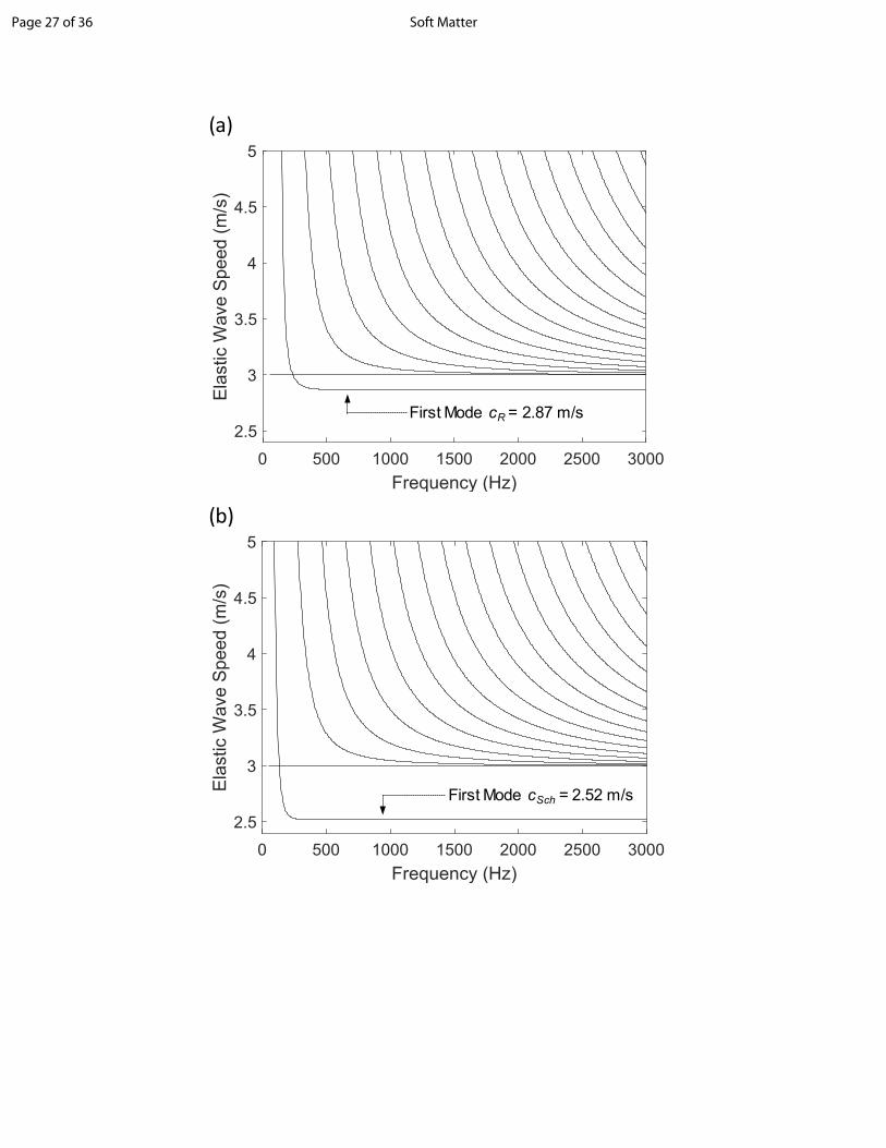
250 From eqn (4) to (12), the components of the local displacement and stress tensor are expressed in

251 the matrix form:

252 [ 𝑢𝑥𝑢𝑧𝜎𝑧𝑧𝜎𝑥𝑧

] = 𝑖𝑫[𝐴𝐿 +𝐴𝐿 ―𝐴𝑆 +𝐴𝑆 ―

]exp [𝑖 (𝑘𝑥𝑥 ― 𝜔𝑡)]

253 where

254 𝑫 = [ 𝑘𝑥𝑒𝑖𝑘𝐿𝑧𝑧 𝑘𝑥𝑒 ―𝑖𝑘𝐿

𝑧𝑧 ― 𝑘𝑆𝑧𝑒𝑖𝑘𝑆

𝑧𝑧 𝑘𝑆𝑧𝑒 ―𝑖𝑘𝑆

𝑧𝑧

𝑘𝐿𝑧𝑒𝑖𝑘𝐿

𝑧𝑧 ― 𝑘𝐿𝑧𝑒 ―𝑖𝑘𝐿

𝑧𝑧 𝑘𝑥𝑒𝑖𝑘𝑆𝑧𝑧 𝑘𝑥𝑒 ―𝑖𝑘𝑆

𝑧𝑧

𝑖𝜌(𝜔2 ― 2𝛼2𝑆𝑘2

𝑥)𝑒𝑖𝑘𝐿𝑧𝑧 𝑖𝜌(𝜔2 ― 2𝛼2

𝑆𝑘2𝑥)𝑒 ―𝑖𝑘𝐿

𝑧𝑧 2𝑖𝜌𝑘𝑥𝑘𝑆𝑧𝛼2

𝑆𝑒𝑖𝑘𝑆𝑧𝑧 ―2𝑖𝜌𝑘𝑥𝑘𝑆

𝑧𝛼2𝑆𝑒 ―𝑖𝑘𝑆

𝑧𝑧

2𝑖𝜌𝑘𝑥𝑘𝐿𝑧𝛼2

𝑆𝑒𝑖𝑘𝐿𝑧𝑧 ―2𝑖𝜌𝑘𝑥𝑘𝐿

𝑧𝛼2𝑆𝑒 ―𝑖𝑘𝐿

𝑧𝑧 ―𝑖𝜌(𝜔2 ― 2𝛼2𝑆𝑘2

𝑥)𝑒𝑖𝑘𝑆𝑧𝑧 ―𝑖𝜌(𝜔2 ― 2𝛼2

𝑆𝑘2𝑥)𝑒 ―𝑖𝑘𝑆

𝑧𝑧]

255 (13)

256 The local displacement vector in the water layer can be expressed in terms of a potential function

257 by the relationship:𝜙𝑤

258 , (14) 𝒖𝒘 = ∇𝜙𝑤

259 which is a special case of eqn (10) where the vector potential , related to the shear partial waves, vanishes.𝜓

260 The scalar potential in eqn (14) must satisfy the wave equation

261 (15)∇2𝜙𝑤 + (𝑘𝑤)2𝜙𝑤 = 0


12

262 where is the wavenumber of the compressional wave in the water layer that comprises (𝑘𝑤)2 = 𝑘2𝑥 + (𝑘𝑤

𝑧 )2

263 the components and in x- and z-directions and has the relation with the compressional wave speed 𝑘𝑥 𝑘𝑤𝑧 𝑘𝑤

264 as 1481 m/s in water. The water layer is treated as a half-space without wave sources. As = 𝜔/𝑐𝑤 𝑐𝑤 =

265 such, only partial waves travelling in the negative z-direction exist, as illustrated in Fig. 3. In addition, we

266 seek guided elastic wave solutions in the soft plate that travel at the water-plate interface as interface

267 waves62-64, so the scalar potential can be expressed with the amplitude and the wavenumber by𝐴𝑤𝐿 ― 𝑘𝑥

268 (16)𝜙𝑤 = (𝐴𝑤𝐿 ― 𝑒 ―𝑖𝑘𝑤

𝑧 𝑧)exp [𝑖 (𝑘𝑥𝑥 ― 𝜔𝑡)]

269 From eqn (11), (12), (14) and (16), the displacement and the pressure (equivalent to the normal

270 stresses in solids) in the vertical direction in the water layer, and , can be derived𝑢𝑤𝑧 𝑝

271 (17)𝑢𝑤𝑧 = ―𝑖(𝑘𝑤

𝑧 𝑒 ―𝑖𝑘𝑤𝑧 𝑧)𝐴𝑤

𝐿 ― exp [𝑖(𝑘𝑥𝑥 ― 𝜔𝑡)]

272 (18)𝑝 = 𝑖(𝑖𝜌𝑤𝜔2𝑒 ―𝑖𝑘𝑤𝑧 𝑧)𝐴𝑤

𝐿 ― exp [𝑖(𝑘𝑥𝑥 ― 𝜔𝑡)]

273 Since the water layer was assumed to be an inviscid liquid that does not support the propagation of

274 shear waves, the shear stress in the water layer is zero, .𝜎𝑤𝑥𝑧 = 0

275 Five boundary conditions are needed to solve for the unknown coefficients for the potential

276 functions in the soft plate and water layers. The boundary conditions include zero displacement at the

277 bottom surface of the soft plate, , due to the rigid glass substratum, continuity of the 𝑢𝑥|𝑧 = ℎ = 𝑢𝑧|𝑧 = ℎ = 0

278 vertical displacements between the soft plate and the water layer, , continuity of the 𝑢𝑧|𝑧 = 0 = 𝑢𝑤𝑧 |𝑧 = 0

279 normal traction in the soft plate and the pressure in the water, , and zero shear traction at 𝜎𝑧𝑧|𝑧 = 0 = 𝑝|𝑧 = 0

280 the interface between the soft plate and the water layer, . Applying these conditions leads to 𝜎𝑥𝑧|𝑧 = 0 = 0

281 five equations for the potential function coefficients, which are expressed below in the matrix form


13

282 [ 𝑘𝑥𝑒𝑖𝑘𝐿𝑧ℎ 𝑘𝑥𝑒 ―𝑖𝑘𝐿

𝑧ℎ ― 𝑘𝑆𝑧𝑒𝑖𝑘𝑆

𝑧ℎ 𝑘𝑆𝑧𝑒 ―𝑖𝑘𝑆

𝑧ℎ 0𝑘𝐿

𝑧𝑒𝑖𝑘𝐿𝑧ℎ ― 𝑘𝐿

𝑧𝑒 ―𝑖𝑘𝐿𝑧ℎ 𝑘𝑥𝑒𝑖𝑘𝑆

𝑧ℎ 𝑘𝑥𝑒 ―𝑖𝑘𝑆𝑧ℎ 0

𝑖𝜌(𝜔2 ― 2𝛼2𝑆𝑘2

𝑥) 𝑖𝜌(𝜔2 ― 2𝛼2𝑆𝑘2

𝑥) 2𝑖𝜌𝑘𝑥𝑘𝑆𝑧𝛼2

𝑆 ―2𝑖𝜌𝑘𝑥𝑘𝑆𝑧𝛼2

𝑆 ―𝑖𝜌𝑤𝜔2

2𝑖𝜌𝑘𝑥𝑘𝐿𝑧𝛼2

𝑆 ―2𝑖𝜌𝑘𝑥𝑘𝐿𝑧𝛼2

𝑆 ―𝑖𝜌(𝜔2 ― 2𝛼2𝑆𝑘2

𝑥) ―𝑖𝜌(𝜔2 ― 2𝛼2𝑆𝑘2

𝑥) 0𝑘𝐿

𝑧 ― 𝑘𝐿𝑧 𝑘𝑥 𝑘𝑥 𝑘𝑤

𝑧

][𝐴𝐿 +𝐴𝐿 ―𝐴𝑆 +𝐴𝑆 ―𝐴𝑤

𝐿 ―] = 𝟎

283 or

284 (19)𝑺𝑨 = 𝟎

285 To obtain non-trivial solutions for from eqn (19), the determinant of the coefficient matrix must 𝑨 𝑺

286 equal to zero:

287 (20)det (𝑺) = 0

288 which is the characteristic equation of the layered model. The solutions of eqn (20) yield the (𝜔,𝑘𝑥)

289 dispersion relation of the guided elastic waves in the water-loaded viscoelastic layer as the speed of the

290 elastic wave propagating along the x-direction, .𝑐 = 𝜔/𝑘𝑥

291

292 3. Results and discussion

293

294 3.1. Numerical simulation

295 In this section, we present a set of dispersion curves predicted by the model for the guided elastic waves in

296 the layered structure under different boundary conditions and mechanical properties as shown in Fig. 4.

297 Each dispersion curve represents a unique elastic wave mode associated with a group of the solutions (𝜔,

298 of eqn (20). Although there are an infinite number of dispersion curves for the model since the frequency 𝑘𝑥)

299 can go to infinity, we only plotted the curves within the frequency range 0-3000 Hz. First, we calculated

300 the dispersion curves for a purely elastic plate with the mechanical properties and geometry such as

301 compressional wave speed 1481 m/s, shear wave speed 3 m/s, zero complex viscosities 𝑐𝐿 = 𝑐𝑆 = 𝜂𝜆 = 𝜂𝜇

302 , and layer thickness h = 10 mm. The compressional wave speed in the gel was assumed to be the same = 0


14

303 as found in water because of the low concentration of agar in the gel phantoms. The large ratio of the

304 compressional to the shear wave speeds corresponds to a Poisson’s ratio of 0.5.

305 Fig. 4a shows the results from the stress-free and clamped boundary conditions imposed on the top

306 and the bottom surfaces of the agarose layer, in which the water layer in Fig. 3 was replaced by vacuum.

307 Except for the non-dispersive mode with a frequency-independent phase velocity , corresponding to the 𝑐𝑆

308 bulk shear wave propagation, each dispersion curve has a cut-off frequency (fc) below which the associated

309 elastic wave mode does not propagate. The cut-off frequencies occur at values of fc = 58, etc. 𝑐𝑆

2ℎ, 𝑐𝑆

ℎ , 3𝑐𝑆

2ℎ , 2𝑐𝑆

ℎ

310 where the phase velocity tends to approach infinity. An implication of the infinite phase velocity at the cut-

311 off frequency is that all points on the free surface of the layer vibrates in phase, leading to a shear-thickness

312 resonance. We note that the phase velocities of all dispersive modes have decreasing trends with frequency

313 and asymptotically approach the bulk shear wave speed , except for the first mode. The asymptotic value 𝑐𝑆

314 of the first mode is the Rayleigh wave velocity of the layer, = 2.87 m/s. The ratio 0.96 agrees 𝑐𝑅 𝑐𝑅/𝑐𝑆 =

315 with the theoretical prediction for a material that has a Poisson’s ratio of 0.562, 63. The penetration depth of

316 the Rayleigh wave is approximately one wavelength, over which the energy of the wave attenuates to 1/e

317 of its maximum value at the layer surface. As such, the elastic mode reaches the asymptotic value and

318 propagates as a pure surface wave without the interference by the energy reflected from the bottom surface.

319 As an example, consider an agarose gel phantom with thickness 10 mm. When the frequency is larger than

320 500 Hz, the wavelength is 5.7 mm, which is smaller than the thickness of the agarose gel layer.

321 When the agarose gel layer is loaded with water on the top surface, the water loading decreases the

322 Rayleigh wave velocity to the Scholte wave velocity 2.52 m/s as shown in Fig. 4b. The Scholte 𝑐𝑆𝑐ℎ =

323 wave propagates at the interface between the gel and the water layers whose elastic energy is attenuated

324 along the transverse direction as part of the energy couples into the water layer. The ratio 0.84 𝑐𝑆𝑐ℎ/𝑐𝑆 =

325 from our numerical calculation agrees well with analytical predictions62, 63.

326 Fig. 4c shows the dispersion curves predicted by the model for a water-loaded viscoelastic layer of

327 agarose gel. In this calculation, the material properties and the plate geometry remained the same as the


15

328 ones used to obtain the results shown in Fig. 4a and 4b, with the sole exception that the complex shear

329 viscosity was changed to = 0.15 Pa-s. One significant difference between the dispersion curves in Fig. 𝜂𝜇

330 4b and 4c is the increasing bulk shear and Scholte wave velocities in the high-frequency region due to the

331 effect of viscosity, which is of particularly interest in this study. Measurement of the dispersive phase

332 velocity over this region can support characterization of the shear modulus and complex shear viscosity of

333 the agarose gel sample. The dispersion curves also depend on the layer thickness as shown in Fig. 5, where

334 the layer thickness is changed to 1 mm with the same material properties as in Fig. 4c. Comparing Fig. 5

335 with Fig. 4c, the most significant difference is that only three elastic modes are supported in the 1 mm thick

336 layer, which correspond to the lowest interface wave, the bulk shear wave, and the second guided wave

337 modes. The lowest mode in Fig. 5 has a higher cut-off frequency since this frequency is inversely

338 proportional to the layer thickness.

339

340 3.2. Experimental results

341 3.2.1. Agarose gel phantoms

342 Fig. 6 shows experimental dispersion curves obtained for the 1.0% and 2.0% agarose gel phantoms of two

343 thicknesses, 10 mm and 1 mm. The bandwidth of the measured dispersion curves was limited to 5 kHz due

344 to the low signal-to-noise ratio of the OCE B-scans, which stemmed from attenuation of the excited waves

345 above this frequency. Each dispersion curve in Fig. 6 represents the average of nine measurements of the

346 phase velocity versus frequency obtained at random positions in the sample. The error bars represent the

347 standard deviation of these nine measurements. For all the experimental dispersion curves, the coefficient

348 of variation (COV), defined as the ratio of standard deviation to the average value of the phase velocity, is

349 less than 2.5%, suggesting homogeneity of the sample elastic properties. The dispersion curves for the 1

350 mm thick samples have a relatively constant wave speed within the high frequency range. The wavelength

351 of the excited waves in the 1.0% agarose sample, for example, decreased from 1.29 mm to 0.38 mm between

352 the frequency range of 1.2 to 4 kHz, which suggests that the excited wave changed from a guided wave at


16

353 lower frequencies to a Scholte wave at higher frequencies. On the other hand, for the 10 mm thick samples,

354 the Scholte wave mode was supported over the frequency bandwidth of the measurement since the

355 wavelength was smaller than the sample thickness. As observed in the numerically-calculated dispersion

356 curves, the phase velocity of the wave modes obtained in the 10 mm samples increase markedly with

357 frequency due to the complex shear viscosity of the samples. In addition, the average phase velocity

358 increased with the agarose concentration in the gel, as expected.

359 The dispersion curves in Fig. 6b have a decreasing trend in the low-frequency range, indicating that

360 the measured mode belongs to the lowest elastic mode illustrated in Fig. 4. This is a reasonable observation

361 since the Scholte wave was the predominant propagation mode near the interface63, 65. Fig. 7 compares

362 numerical calculations of the dispersion curve for the first mode in the layered model to the experimental

363 data. The shear modulus and complex shear viscosity were used as free fitting parameters in the numerical

364 model for samples of 10 mm thickness, while shear modulus was the only free fitting parameter for samples

365 of 1 mm thickness owing to the limited dispersion observed in these experiments. Good agreement was

366 found between the experimental and numerical results, except for the larger errors observed within the low

367 frequency range in Fig. 7c and 7d, which were due to lack of sufficient periodic cycles of the waves within

368 the OCE field of view to estimate the wavelength through fast Fourier transform. The shortest wavelength

369 below 2 kHz in Fig. 7c and 7d was 1.65 mm; this is equivalent to less than six cycles within the total

370 sampling distance in the OCE B-scan, which limited the accuracy of the wavelength estimation. The best-

371 fit material properties for the samples are listed in Table 1. The shear modulus and viscosity increase, as

372 expected, with the concentration of agarose in the gel. The shear moduli measured from 1 and 10 mm

373 samples were similar at 1.0% and indistinguishable at 2.0%, and the values agree well with those reported

374 in the literature38, 52. This finding validates the use of the layered model to determine the mechanical

375 properties of viscoelastic materials.

376

377 3.2.2. Mixed-culture bacterial biofilm


17

378 After 30 days of growth, the mixed-culture bacterial biofilm reached a ~2.5 mm thickness with a ~ 250 µm

379 variation over a 4 mm lateral extent due to surface roughness as shown in the OCT B-scan (Fig. 8a) that

380 illustrates the sample morphology. The OCE B-scan obtained at an excitation frequency of 660 Hz and the

381 dispersion curves from the numerical simulation and experimental measurements are shown in Fig. 8b and

382 8c, respectively. In order to more precisely calculate the speed of the elastic wave travelling along the

383 curved surface, a cubic function was fitted to the curved region of the biofilm surface to approximate the

384 propagation path of the elastic waves. The amplitudes at discrete intervals along the path were extracted,

385 and the fast Fourier transform was applied to the data to obtain the spatial frequency (or inverse wavelength)

386 of the elastic waves (See Section S4 in the Supplemental Information). The maximal excitation frequency

387 in the measurement was limited to 1 kHz due to attenuation of elastic waves in the sample. Unlike the

388 agarose gel sample, the OCT image of the biofilm shows internal structural variations due to the presence

389 of pores (dark bands), which also results in the low phase amplitude of the elastic waves in the OCE image.

390 This finding aligns with other observations that pores and structural heterogeneity are common in biofilms13,

391 66.

392 The bright white bands in the OCT image (Fig. 8a) indicate the boundary of the biofilm with air,

393 and the propagation mode illustrated in the OCE image (Fig. 8b) is a Rayleigh surface wave. The use of the

394 Rayleigh wave measurement is particularly advantageous in this case since the penetration depths of the

395 wave, 1.2 mm at 550 Hz and 0.76 mm at 1 kHz, were less than the sample thickness and thus less sensitive

396 to sample thickness variations. The dispersion curve for the measured data in Fig. 8c shows a 15% increase

397 in phase velocity within the frequency bandwidth of the measurement. The measured dispersion curve was

398 fitted by the numerical model using the biofilm shear modulus and viscosity as free fitting parameters.

399 Similar to Fig. 7c and 7d, large disagreement between the experimental data and the numerical model is

400 observed within the low frequency range (≤ 400 Hz) due to the limited number of wavelengths within the

401 total sampling distance. The best-fit shear modulus and complex shear viscosity are 429 Pa and 0.06 Pa-s.

402 These estimated properties represent the average bulk viscoelastic properties of the biofilm, and are within

403 the broad range of reported values for the viscoelastic properties of biofilms (shear modulus = 10−1 - 105 Pa


18

404 and viscosity = 10−1 - 1010 Pa-s)18. The broad range reflects both the diversity of different type of biofilms

405 used in other studies and additional differences resulting from the inconsistencies and disadvantages of the

406 characterization methods used. We highlight that most of the rheometry techniques employed for property

407 characterization are destructive or involve large disturbances in sample geometry when testing, which

408 inevitably causes changes of the sample morphology and properties. On contrary, our novel technique has

409 a nondestructive nature that prevents any structural change and allows for the estimation of viscoelastic

410 properties in the intact forms of the samples, which makes this more advantageous compared to other

411 techniques.

412 We remark that in our inverse modeling analysis, we assumed the bulk modulus of the biofilm to

413 be equal to the bulk modulus of water due to high water content (> 90%) of the sample. Overall, this novel

414 approach provides a nondestructive, direct, local and in situ option to interrogate mechanical properties in

415 these type of systems. Further work that refines the layered model is needed to address the heterogeneous

416 spatial distribution of the shear modulus in the sample as suggested in Fig. 8b.

417

418 4. Conclusion

419 We developed methods involving a combination of OCE measurements and inverse modeling to

420 characterize the mechanical properties of soft viscoelastic materials and bacterial biofilms. OCE was

421 employed to obtain the dispersion curve—the frequency-dependent phase velocity—of the surface acoustic

422 wave travelling in a biofilm supported by a rigid substrate. This is the first work to present wave propagation

423 in biofilms, discover the frequency-dependent wave velocity, and interpret the dispersive wave velocity by

424 a theoretical model to estimate the mechanical properties. The theoretical model obtained the dispersion

425 curves of guided elastic wave modes by solving the elastodynamic wave equation for a layered viscoelastic

426 plate attached to a rigid substratum and a semi-infinite water/vacuum layer on both sides. Dispersion in

427 these materials depends on the mechanical properties, the geometry of the plate, and the presence or absence

428 of water on the surface of the viscoelastic material. The model was validated by estimating the shear moduli


19

429 and complex shear viscosities from the OCE measurements of phase velocities in 10 and 1 mm thick agarose

430 gel plates with 1.0% and 2.0% agarose concentrations. The estimation of the agarose gel properties agrees

431 well with the ones in literature. These results suggest that the wave propagation observed in the OCE

432 measurements of agarose gel plates belong to the lowest elastic mode travelling near the top boundary of

433 the plate. The influence of the plate geometry is crucial since the guided waves interact with the bottom

434 boundary when the acoustic wavelength is larger than the plate thickness. We then used this approach to

435 measure the shear modulus and complex shear viscosity in a bacterial biofilm, and obtained reasonable

436 results that are within the range reported in literature. Since there is no “gold standard” measurement for

437 mechanical properties in soft materials and biofilms, our nondestructive technique provides a novel

438 approach for characterizing these properties without affecting the original status of the samples.

439 Furthermore, this framework enhances our understanding of elastic wave propagation in soft viscoelastic

440 materials and provides a first proof-of-concept of OCE application to quantify mechanical properties of

441 biofilms that are critically important in diverse environments and applications. The OCE technique can be

442 further employed to study relationships between biofilm morphology, growth conditions, and elastic

443 properties. Future work should focus on refining the layered model to address variations of the geometry

444 and heterogeneity of material properties in soft materials as well as on utilizing the technique for rapid,

445 nondestructive, spatially-resolved characterization of biofilm mechanical properties across a range of

446 microbial systems and applications.

447

448 Conflicts of interest

449 The authors declare no conflicts of interest.

450

451 Acknowledgements

452 The authors thank Dr. Claire Prada (Institute Langevin, France) for the useful discussion regarding the

453 development of the multi-layered model and Dr. Alex Rosenthal (inCTRL, Canada) for his insights on

454 biofilms and rotating annular reactor operation. The authors also acknowledge the support of the National


20

455 Science Foundation via Award CBET-1701105, and the Civil and Environmental Engineering Department

456 at Northwestern University for providing seed funding for this project.

457

458 REFERENCES

459 1. L. Hall-Stoodley, J. W. Costerton and P. Stoodley, Nat Rev Micro, 2004, 2, 95-108.460 2. J. N. Wilking, T. E. Angelini, A. Seminara, M. P. Brenner and D. A. Weitz, MRS Bulletin, 2011, 461 36, 385-391.462 3. H.-C. Flemming, J. Wingender, U. Szewzyk, P. Steinberg, S. A. Rice and S. Kjelleberg, Nat. Rev. 463 Micro., 2016, 14, 563-575.464 4. J. W. Costerton, Z. B. Lewandowski, D. E. Caldwell, D. R. Korber and H. M. Lappin-Scott, Annu 465 Rev Microbiol, 1995, 49, 711-745.466 5. T. J. Battin, W. T. Sloan, S. Kjelleberg, H. Daims, I. M. Head, T. P. Curtis and L. Eberl, Nat Rev 467 Micro, 2007, 5, 76-81.468 6. T. J. Battin, K. Besemer, M. M. Bengtsson, A. M. Romani and A. I. Packmann, Nat. Rev. Micro., 469 2016, 14, 251-263.470 7. B. Halan, K. Buehler and A. Schmid, Trends Biotechnol, 2012, 30, 453-465.471 8. N. Billings, A. Birjiniuk, T. S. Samad, P. S. Doyle and K. Ribbeck, Rep Prog Phys, 2015, 78, 472 036601.473 9. H. C. Flemming, J. Wingender and U. Szewzyk, Biofilm Highlights, Springer Berlin Heidelberg, 474 2011.475 10. I. Klapper, C. J. Rupp, R. Cargo, B. Purvedorj and P. Stoodley, Biotechnol Bioeng, 2002, 80, 476 289-296.477 11. J. N. Wilking, T. E. Angelini, A. Seminara, M. P. Brenner and D. A. Weitz, MRS Bulletin, 2011, 478 36, 385-391.479 12. S. Bhat, D. Jun, B. C and T. E. S Dahms, in Viscoelasticity - From Theory to Biological 480 Applications, 2012, DOI: 10.5772/49980, ch. Chapter 6.481 13. H. Boudarel, J. D. Mathias, B. Blaysat and M. Grediac, NPJ Biofilms Microbiomes, 2018, 4, 17.482 14. Y. He, B. W. Peterson, M. A. Jongsma, Y. Ren, P. K. Sharma, H. J. Busscher and H. C. van der 483 Mei, PLoS One, 2013, 8, e63750.484 15. M. Bol, A. E. Ehret, A. Bolea Albero, J. Hellriegel and R. Krull, Crit Rev Biotechnol, 2013, 33, 485 145-171.486 16. N. Aravas and C. S. Laspidou, Biotechnol Bioeng, 2008, 101, 196-200.487 17. A. K. Ohashi, T.; Syutsubo, K.; Harada, H., Water Sci. & Technol., 1999, 39, 261-268.488 18. B. W. Peterson, Y. He, Y. Ren, A. Zerdoum, M. R. Libera, P. K. Sharma, A. J. van Winkelhoff, 489 D. Neut, P. Stoodley, H. C. van der Mei and H. J. Busscher, FEMS Microbiol Rev, 2015, 39, 234-490 245.491 19. P. Stoodley, K. Sauer, D. G. Davies and J. W. Costerton, Annu Rev Microbiol, 2002, 56, 187-209.492 20. E. C. Hollenbeck, C. Douarche, J. M. Allain, P. Roger, C. Regeard, L. Cegelski, G. G. Fuller and 493 E. Raspaud, J Phys Chem B, 2016, 120, 6080-6088.494 21. O. Galy, P. Latour-Lambert, K. Zrelli, J. M. Ghigo, C. Beloin and N. Henry, Biophys J, 2012, 495 103, 1400-1408.496 22. V. Korstgens, H. C. Flemming, J. Wingender and W. Borchard, J Microbiol Methods, 2001, 46, 497 9-17.498 23. B. W. Towler, C. J. Rupp, A. B. Cunningham and P. Stoodley, Biofouling, 2003, 19, 279-285.499 24. S. Aggarwal, E. H. Poppele and R. M. Hozalski, Biotechnol Bioeng, 2010, 105, 924-934.


21

500 25. D. N. Hohne, J. G. Younger and M. J. Solomon, Langmuir, 2009, 25, 7743-7751.501 26. J. D. Mathias and P. Stoodley, Biofouling, 2009, 25, 695-703.502 27. P. C. Lau, J. R. Dutcher, T. J. Beveridge and J. S. Lam, Biophys J, 2009, 96, 2935-2948.503 28. F. C. Cheong, S. Duarte, S.-H. Lee and D. G. Grier, Rheologica Acta, 2008, 48, 109-115.504 29. A. Manduca, T. E. Oliphant, M. A. Dresner, J. L. Mahowald, S. A. Kruse, E. Amromin, J. P. 505 Felmlee, J. F. Greenleaf and R. L. Ehman, Med Image Anal, 2001, 5, 237-254.506 30. T. A. Krouskop, T. M. Wheeler, F. Kallel, B. S. Garra and T. Hall, Ultrasonic imaging, 1998, 20, 507 260-274.508 31. J. Ophir, I. Cespedes, H. Ponnekanti, Y. Yazdi and X. Li, Ultrasonic imaging, 1991, 13, 111-134.509 32. B. F. Kennedy, K. M. Kennedy and D. D. Sampson, IEEE Journal of Selected Topics in Quantum 510 Electronics, 2014, 20, 272-288.511 33. X. Liang, V. Crecea and S. A. Boppart, J Innov Opt Health Sci, 2010, 3, 221-233.512 34. M. Wagner and H. Horn, Biotechnol Bioeng, 2017, 114, 1386-1402.513 35. X. Liang, S. G. Adie, R. John and S. A. Boppart, Opt Express, 2010, 18, 14183-14190.514 36. L. Ambrozinski, S. Song, S. J. Yoon, I. Pelivanov, D. Li, L. Gao, T. T. Shen, R. K. Wang and M. 515 O'Donnell, Sci Rep, 2016, 6, 38967.516 37. M. Razani, T. W. Luk, A. Mariampillai, P. Siegler, T. R. Kiehl, M. C. Kolios and V. X. Yang, 517 Biomed Opt Express, 2014, 5, 895-906.518 38. S. Song, Z. Huang, T. M. Nguyen, E. Y. Wong, B. Arnal, M. O'Donnell and R. K. Wang, J 519 Biomed Opt, 2013, 18, 121509.520 39. S. Song, N. M. Le, Z. Huang, T. Shen and R. K. Wang, Opt Lett, 2015, 40, 5007-5010.521 40. Q. Wang, G. Jiang, L. Ye, M. Pijuan and Z. Yuan, Water Res, 2014, 62, 202-210.522 41. J. Zhu, Y. Qu, T. Ma, R. Li, Y. Du, S. Huang, K. K. Shung, Q. Zhou and Z. Chen, Opt Lett, 2015, 523 40, 2099-2102.524 42. V. Crecea, A. L. Oldenburg, X. Liang, T. S. Ralston and S. A. Boppart, Opt Express, 2009, 17, 525 23114-23122.526 43. P. C. Huang, P. Pande, A. Ahmad, M. Marjanovic, D. R. Spillman, Jr., B. Odintsov and S. A. 527 Boppart, IEEE J Sel Top Quantum Electron, 2016, 22.528 44. S. Wang, A. L. Lopez, 3rd, Y. Morikawa, G. Tao, J. Li, I. V. Larina, J. F. Martin and K. V. Larin, 529 Biomed Opt Express, 2014, 5, 1980-1992.530 45. R. M. Donlan, Emerg Infect Dis, 2002, 8, 881-890.531 46. J. Wimpenny, W. Manz and U. Szewzyk, FEMS Microbiol Rev, 2000, 24, 661-671.532 47. J. W. Costerton, Z. Lewandowski, D. E. Caldwell, D. R. Korber and H. M. Lappin-Scott, Annu 533 Rev Microbiol, 1995, 49, 711-745.534 48. H.-C. Flemming, in Biofilm Highlights, eds. H.-C. Flemming, J. Wingender and U. Szewzyk, 535 Springer Berlin Heidelberg, Berlin, Heidelberg, 2011, DOI: 10.1007/978-3-642-19940-0_5, pp. 536 81-109.537 49. V. D. Gordon, M. Davis-Fields, K. Kovach and C. A. Rodesney, Journal of Physics D: Applied 538 Physics, 2017, 50, 223002.539 50. WEF, WEF Manual of Practice 35: Biofilm Reactors, WEF Press, Alexandria, VA, 2011.540 51. A. F. Rosenthal, J. S. Griffin, M. Wagner, A. I. Packman, O. Balogun and G. F. Wells, Biotechnol 541 Bioeng, 2018, 115, 2268-2279.542 52. M. Couade, M. Pernot, C. Prada, E. Messas, J. Emmerich, P. Bruneval, A. Criton, M. Fink and 543 M. Tanter, Ultrasound Med Biol, 2010, 36, 1662-1676.544 53. J. Laperre and W. Thys, The Journal of the Acoustical Society of America, 1993, 94, 268-278.545 54. Z. Zhu and J. Wu, The Journal of the Acoustical Society of America, 1995, 98, 1057-1064.546 55. F. Simonetti, The Journal of the Acoustical Society of America, 2004, 115, 2041-2053.547 56. J. D. Achenbach, in Wave Propagation in Elastic Solids, ed. J. D. Achenbach, Elsevier, 548 Amsterdam, 1975, DOI: 10.1016/b978-0-7204-0325-1.50008-4, pp. 79-121.549 57. M. J. S. Lowe, IEEE Transactions on Ultrasonics, Ferroelectrics and Frequency Control, 1995, 550 42, 525-542.


22

551 58. J. L. Rose, Ultrasonic Waves in Solid Media, Cambridge University Press, 1999.552 59. N. A. Haskell, Bulletin of the Seismological Society of America, 1953, 43, 17-34.553 60. B. Pavlakovic, M. Lowe, D. Alleyne and P. Cawley, in Review of Progress in Quantitative 554 Nondestructive Evaluation, eds. D. O. Thompson and D. E. Chimenti, Springer US, Boston, MA, 555 1997, DOI: 10.1007/978-1-4615-5947-4_24, ch. Chapter 24, pp. 185-192.556 61. W. T. Thomson, Journal of Applied Physics, 1950, 21, 89-93.557 62. M. A. Kirby, I. Pelivanov, S. Song, L. Ambrozinski, S. J. Yoon, L. Gao, D. Li, T. T. Shen, R. K. 558 Wang and M. O'Donnell, J Biomed Opt, 2017, 22, 1-28.559 63. I. A. Viktorov, Rayleigh and Lamb Waves, Springer US, 1 edn., 1967.560 64. J. Zhu, J. S. Popovics and F. Schubert, The Journal of the Acoustical Society of America, 2004, 561 116, 2101-2110.562 65. C. B. Scruby and L. E. Drain, Laser Ultrasonics Techniques and Applications, Taylor & Francis, 563 1990.564 66. M. Jafari, P. Desmond, M. C. M. van Loosdrecht, N. Derlon, E. Morgenroth and C. Picioreanu, 565 Water Res, 2018, 145, 375-387.

566


Figures

Nondestructive Characterization of Soft Materials and Biofilms by

Measurement of Guided Elastic Wave Propagation Using Optical Coherence

Elastography

Hong-Cin Liou1, Fabrizio Sabba2, Aaron Packman2, George Wells2, Oluwaseyi Balogun1,2*

1Mechanical Engineering Department, Northwestern University, Evanston, IL 60208

2Civil and Environmental Engineering Department, Northwestern University, Evanston, IL

60208

*Corresponding author:

Oluwaseyi Balogun, Phone: +1 847-491-3054; e-mail: [email protected]


Fig. 1. Phase-sensitive optical coherence elastography setup


1 mm

Selected wave path

- /2

- /4

0

/4

/2

Pha

se (r

ad)

1 mm

x

z

Air

Water

Agarose Gel

(a)

(b)

Fig. 2. (a) Optical coherence tomography image of a 2.0% agarose gel phantom. The thickness of the water layer was reduced in this figure for visualization purposes. The experiments were conducted with a water layer of >2 mm thickness. (b) Optical coherence elastography image showing phase distribution of 1.4 kHz elastic waves in the sample. The pixel sizes along the x- and z-directions are 4 and 2 m.


Agarose

WaterL−

L− S− L+ S+ hz

x

Fig. 3. Geometry of the layered numerical model. Symbols L and S represent compressional and shear waves. Positive and negative superscripts are used to represent forward and backward propagating partial waves.


(a)

0 500 1000 1500 2000 2500 3000Frequency (Hz)

2.5

3

3.5

4

4.5

5

Elas

tic W

ave

Spee

d (m

/s)

First Mode cR = 2.87 m/s

(b)

0 500 1000 1500 2000 2500 3000Frequency (Hz)

2.5

3

3.5

4

4.5

5

Elas

tic W

ave

Spee

d (m

/s)

First Mode cSch = 2.52 m/s


0 500 1000 1500 2000 2500 3000Frequency (Hz)

2.5

3

3.5

4

4.5

5

Elas

tic W

ave

Spee

d (m

/s)

(c)

Fig. 4. Dispersion curves for (a) a pure-elastic layer with free-clamped boundary condition, (b) a pure-elastic plate with liquid loading on the top surface and clamped boundary condition at bottom surface, and (c) a viscoelastic layer with liquid loading and clamped boundary conditions. The layer thickness h =10 mm.


0 500 1000 1500 2000 2500 3000Frequency (Hz)

2.5

3

3.5

4

4.5

5

Ela

stic

Wav

e S

peed

(m/s

)

1st Interface Mode Transverse Wave Mode 2nd Guided Wave Mode

Fig. 5. Dispersion curves for a 1 mm thick viscoelastic layer with liquid loading and clamped boundary conditions.


(a)

1000 1500 2000 2500 3000 3500 4000Frequency (Hz)

1.4

1.45

1.5

1.55

1.6

1.65E

last

ic W

ave

Spe

ed (m

/s)

Thickness = 10 mmThickness = 1 mm


(b)

1000 1500 2000 2500 3000 3500 4000 4500 5000Frequency (Hz)

2.8

3

3.2

3.4

3.6

3.8

4E

last

ic W

ave

Spe

ed (m

/s)

Thickness = 10 mmThickness = 1 mm

Fig. 6. Measured guided elastic wave dispersion curves in agarose gel phantoms with (a) 1.0% and (b) 2.0% agarose concentrations, for different sample thicknesses.


(a)

1000 1500 2000 2500 3000 3500 4000Frequency (Hz)

1.4

1.45

1.5

1.55

1.6

1.65

1.7

Elas

tic W

ave

Spee

d (m

/s)

ModelExperiment

(b)

1000 1500 2000 2500 3000 3500 4000Frequency (Hz)

1.5

1.52

1.54

1.56

1.58

1.6

Elas

tic W

ave

Spee

d (m

/s)

ModelExperiment


(c)

1000 1500 2000 2500 3000 3500 4000 4500 5000Frequency (Hz)

2.9

3

3.1

3.2

3.3

3.4

3.5

Ela

stic

Wav

e S

peed

(m/s

)

ModelExperiment

(d)

1000 1500 2000 2500 3000 3500 4000 4500 5000Frequency (Hz)

2.9

3

3.1

3.2

3.3

3.4

3.5

3.6

3.7

3.8

Elas

tic W

ave

Spee

d (m

/s)

ModelExperiment

Fig. 7. Comparison of measured and numerical guided elastic wave dispersion curves in gel samples with 1.0% (a and b), and 2.0% (c and d) agarose concentrations, for different sample thicknesses. Sample thickness = 10 mm in (a) and (c), and 1 mm in (b) and (d). Model parameters are listed in Table 1.


Sample Properties (a) (b) (c) (d)

Agarose gel concentration 1.0% 2.0%Thickness (mm) 10 1 10 1Shear Wave Speed (m/s) 1.71 1.81 3.55 3.55Complex Shear Viscosity (Pa-s) 0.07 0.22Shear Modulus (kPa) 2.9 3.2 12.6 12.6

Table 1: Estimated mechanical properties for agarose gel phantoms by model


1 mm

Selected wave path

- /2

- /4

0

/4

/2

Phas

e (ra

d)

1mm

(a)

(b)

100 200 300 400 500 600 700 800 900 1000Frequency (Hz)

0.6

0.65

0.7

0.75

0.8

0.85

0.9

0.95

1

Ela

stic

Wav

e S

peed

(m/s

)

ModelExperiment

(c)


Fig. 8. (a) Optical coherence tomography image of a mixed-culture bacterial biofilm, (b) optical coherence elastography image showing phase distribution of 660 Hz elastic waves in the sample, and (c) dispersion curves for the model (shear modulus 429 Pa and complex shear viscosity 0.06 Pa-s) and excited elastic waves in the sample.


Nondestructive Characterization of Soft Materials and ...

Documents

Transcript of Nondestructive Characterization of Soft Materials and ...