Non-Walrasian Labor Markets I: The McCall Search Model · PDF fileOutlineMotivationTwo models...

Outline Motivation Two models McCall’s model Waiting times Average dynamics Steady state

Non-Walrasian Labor Markets I: TheMcCall Search Model

Timothy Kam

School of Economics & CAMAAustralian National University

ECON8022, This version May 28, 2008


Outline

1 Motivation

2 Two models

3 McCall’s modelGeneral descriptionDecision problemEffect of mean-preserving spreadLayoffs

4 Waiting times

5 Average dynamics

6 Steady state


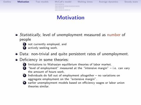
Motivation

Statistically, level of unemployment measured as number ofpeople

1 not currently employed, and2 actively seeking work.

Data: non-trivial and quite persistent rates of unemployment.

Deficiency in some theories:1 limitations to Walrasian equilibrium theories of labor market.2 “level of employment” measured at the “intensive margin” – i.e. can vary

the amount of hours work.3 Individuals do fall out of employment altogether – no variations on

aggregate employment on the “extensive margin”.4 earlier unemployment models based on efficiency wages or labor union

theories similar.


An alternative theory:

Heterogenous goods (labor) with no single marketplace toclear excess demand or supply; and

Parties to a trade must search for someone to trade with.

Double coincidence of wants problem.

i.e. involve transactions costs – it takes time for a person to lookfor a job and it takes time for a vacancy to find a worker.

Search frictions can potentially rationalize significant transit timesbetween unemployment and employment in a equilibrium wheremarkets do not necessarily need to clear.


We will look at two basic models:

1 one-sided, partial-equilibrium models of job search: McCall(1970) – an optimal stopping time example.

2 Mortensen (1982), Pissarides (2000) and Diamond (1982)search and matching model.

Here we will apply stochastic DP techniques we have learned.

Extensions: see recent survey of the state of the literature, seeRogerson, Shimer, and Wright (2004).


McCall one-sided search

Features:

1 Representative unemployed worker’s Markov decision problem.

2 Worker faces given distribution of job offers per period.

3 Binary choice: accept/reject.

4 If accept stay in job forever (or may be laid of in eachsubsequent period with some probability).

5 If reject, take compensation payout, and wait to search nextperiod.

6 Implications for aggregate/average unemployment dynamics.


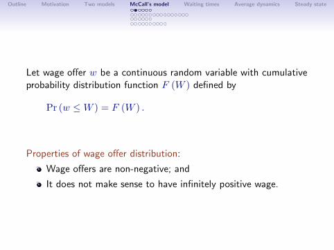
Let wage offer w be a continuous random variable with cumulativeprobability distribution function F (W ) defined by

Pr (w ≤W ) = F (W ) .

Properties of wage offer distribution:

Wage offers are non-negative; and

It does not make sense to have infinitely positive wage.


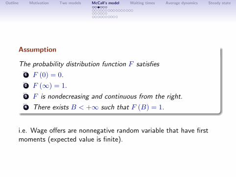
Assumption

The probability distribution function F satisfies

1 F (0) = 0.

2 F (∞) = 1.3 F is nondecreasing and continuous from the right.

4 There exists B < +∞ such that F (B) = 1.

i.e. Wage offers are nonnegative random variable that have firstmoments (expected value is finite).


The expected value or mean of w is

E (w) =∫ B

0wdF (w)

Note we can integrate by parts:∫ B

0wdF (w) = wF (w)|B0 −

∫ B

0F (w) dw

= B −∫ B

0F (w) dw

so we can also write

E (w) = B −∫ B

0F (w) dw.


Example

Consider event of independent drawing of w1 and w2 that are lessthan w from distribution F : i.e. the event{(w1 < w) ∩ (w2 < w)} . Then

Pr {(w1 < w) ∩ (w2 < w)} = Pr {max (w1, w2) < w}= F (w)2

The random variable max (w1, w2) has mean

E [max (w1, w2)] = B −∫ B

0F (w)2 dw.


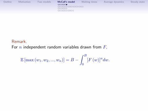
Remark.For n independent random variables drawn from F,

E [max (w1, w2, ..., wn)] = B −∫ B

0[F (w)]ndw.


The decision problem

Each period worker draws offer w from fixed wage distributionF (W ) = Pr (w ≤W ).

F (W ) satisfies Assumption 1.

Worker’s income per period is yt.

worker can reject w this period and keep searching – i.e. waitfor next period offer w′. Meanwhile receives unemploymentcompensation, yt = c.

or, he can accept w and receives yt = w per period forever(no quits or firing).

worker has no recall.


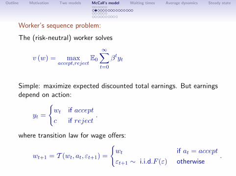
Worker’s sequence problem:

The (risk-neutral) worker solves

v (w) = maxaccept,reject

E0

∞∑t=0

βtyt

Simple: maximize expected discounted total earnings. But earningsdepend on action:

yt =

{wt if accept

c if reject.

where transition law for wage offers:

wt+1 = T (wt, at, εt+1) =

{wt if at = accept

εt+1 ∼ i.i.d.F (ε) otherwise.


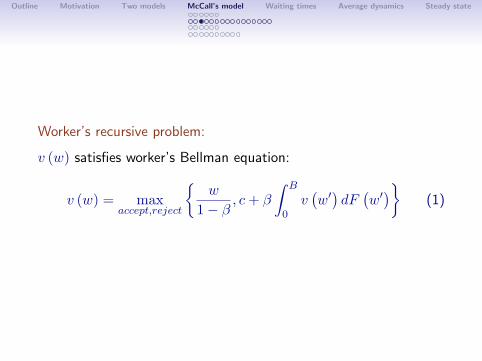
Worker’s recursive problem:

v (w) satisfies worker’s Bellman equation:

v (w) = maxaccept,reject

{w

1− β, c+ β

∫ B

0v(w′)dF(w′)}

(1)


Worker’s optimal policy function:

The optimal action ∈ {accept, reject} is characterized by:

v (w) =

{c+ β

∫ B0 v (w′) dF (w′) := w

1−β if w < ww

1−β if w ≥ w(2)


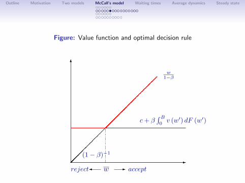
Figure: Value function and optimal decision rule

6

-(1− β)−1

w1−β

c+ β∫ B0v (w′) dF (w′)

w


Figure: Value function and optimal decision rule

6

-(1− β)−1

w1−β

c+ β∫ B0v (w′) dF (w′)

w accept-reject�


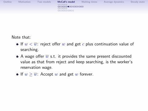
Note that:

If w < w: reject offer w and get c plus continuation value ofsearching.

A wage offer w s.t. it provides the same present discountedvalue as that from reject and keep searching, is the worker’sreservation wage.

If w ≥ w: Accept w and get w forever.


At the optimal reservation wage, w,

w

1− β= c+ β

∫ B

0v(w′)dF(w′)

is equivalent to, after some manipulation,

w − c =β

1− β

∫ B

w

(w′ − w

)dF(w′).

LHS ≡ cost of being unemployed at current offer w and searchingagain next period. RHS ≡ expected present value benefit ofsearching one more time in terms of drawing w′ > w.


w − c =β

1− β

∫ B

w

(w′ − w

)dF(w′).

Jonesy says: “This is just Cost-Benefit Analysis!”


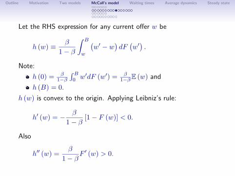
Let the RHS expression for any current offer w be

h (w) ≡ β

1− β

∫ B

w

(w′ − w

)dF(w′).

Note:

h (0) = β1−β

∫ B0 w′dF (w′) = β

1−βE (w) and

h (B) = 0.

h (w) is convex to the origin. Applying Leibniz’s rule:

h′ (w) = − β

1− β[1− F (w)] < 0.

Also

h′′ (w) =β

1− βF ′ (w) > 0.


Exercise

Draw a diagram showing w − c = β1−β

∫ Bw (w′ − w) dF (w′) .

What happens to the solution w if the government increasesunemployment benefits c exogenously?


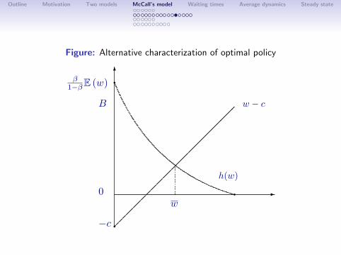
Figure: Alternative characterization of optimal policy

6

-

q

q

qw

h(w)

w − c

−c

0

B

β1−βE (w)


What is mean preserving spread?

Useful for experimenting with “turbulence in economy”.Interpret as riskiness has increased (in downturns), holdingaverage wage offer constant.

Consider a family of distributions that have the same mean.

We can index distributions in this class by a parameter r ∈ R,where R is some arbitrary index set.

So the rth distribution in our family of distributions withidentical mean is denoted by

Pr (w ≤W ) = F (W, r) .


Assumption

The class of probability distribution functions {F (W, r)}r∈R hasthe property that:

1 F (W, r) is differentiable w.r.t. r for all W ∈ [0, B].2 F (0, r) = 0 for all r ∈ R.3 There is a single B < +∞ such that F (B, r) = 1 for allr ∈ R.


Consider R an uncountable set.

Definition

An increase in r represents a mean-preserving increase in risk if∫ B

0

∂F (w, r)∂r

dw = 0 (3)

and ∫ y

0

∂F (w, r)∂r

dw ≥ 0, 0 ≤ y ≤ B. (4)


In words, what we want in mean-preserving spread is:

1 Expected value of the r.v. is unchanged as we switch“infinitesimally” from one distribution r to another r + ∂r.

2 But this is done by putting “more mass on the tails” of thedistribution.


Effect of mean-preserving spreadFor another way to see how w is determined we go back to theequation

w − c =β

1− β

∫ B

w

(w′ − w

)dF(w′).

which equates the cost to the benefit of searching.


This can be re-written as

w − (1− β) c = βE (w)− β∫ w

0

(w′ − w

)dF(w′)

Exercise

Show that∫ w

0

(w′ − w

)dF(w′)

= −∫ w

0F(w′)dw′.

Hint: Let u = (w′ − w) and v = F (w′). Use integration by partsformula,

∫udv = uv −

∫vdu.


We use this to show that w can be characterized by:

w − c = β [E (w)− c]− β∫ w

0

(w′ − w

)dF(w′)

= β [E (w)− c] + β

∫ w

0F(w′)dw′.


Let g (w) =∫ w0 F (w′) dw′. Note:

g (0) = 0,g (w) ≥ 0,g′ (w) = F (w) > 0,g′′ (w) = F ′ (w) > 0, for w > 0.

Then we can write

w − c = β [E (w)− c] + β

∫ w

0F(w′)dw′

≡ β [E (w)− c] + βg (w) .


w − c = β [E (w)− c] + β

∫ w

0F(w′)dw′

≡ β [E (w)− c] + βg (w) .

OK, so what is the effect of a mean preserving spread on thismodel?

By definition of MPS in (4), applying it here to the function g,

conclude as we increase MPS , r, we increase g.

So this shifts βg (w) up.

Therefore resulting w increases.


LayoffsConsider the same setup as before.

Now assume after the first period on the job, there is a probabilityα ∈ (0, 1) of being laid off.

For simplicity, assume α independent of tenure. When employed,the worker receives w per period until fired.

Conclude that value function with α > 0 is strictly dominated byvalue function when α = 0.


Specifically, the Bellman equation is now

v̂ (w) =

max{w + β

[(1− α) v̂ (w) + α

(c+ β

∫v̂(w′′)dF(w′′))]

,

c+ β

∫v̂(w′)dF(w′)}

.


Exercise

Show that v̂ (w) defines a unique value function satisfying theBellman equation and it is a nondecreasing function in w.

Hint: Show that the Bellman equation defines an operator T thatmaps a set of bounded and continuous functions into itself; thenshow that T is a contraction map with modulus β on a completemetric space. (What is the metric?) Then show that v is constantif the action is reject, and strictly increasing, since per-periodutility is strictly increasing, if the action is accept.


So solution of the reservation wage form:

v̂ (w) =

{w+βα(c+β

R bv(w′′)dF (w′′))1−β(1−α) , if w ≥ w

c+ β∫v̂ (w′) dF (w′) , if w < w

where w solves

w + βα(c+ β

∫v̂ (w′′) dF (w′′)

)1− β (1− α)

= c+ β

∫v̂(w′)dF(w′).

Note: E[v̂(w′′)] = E[v̂(w′)]. Why?


Rearranging,

w

1− β= c+ β

∫v̂(w′)dF(w′)

(*)

Contrast this with the reservation wage in the model previouslywhere there is no risk of layoffs, α = 0:

w

1− β= c+ β

∫ B

0v(w′)dF(w′)

(5)

The difference now is that v̂ (w′) 6= v (w′). The two value functionare not the same! In particular, v̂ (w) < v (w) .


Proposition

v̂ (w) < v (w) .


Proof.

Consider the more general case where per-period utility isU : [0, B]→ R, and U ′ is everywhere positive.Then

v̂ (w) =

1

1−β(1−α) [U(w) + βαv̂(0)] , if w ≥ w

v̂(0), if w < w

where:

v̂(0) = U(c) + β

∫v̂(w′)dF(w′)

:=U(w)1− β

.


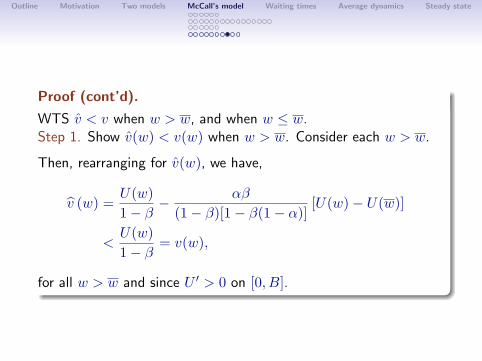
Proof (cont’d).

WTS v̂ < v when w > w, and when w ≤ w.Step 1. Show v̂(w) < v(w) when w > w. Consider each w > w.

Then, rearranging for v̂(w), we have,

v̂ (w) =U(w)1− β

− αβ

(1− β)[1− β(1− α)][U(w)− U(w)]

<U(w)1− β

= v(w),

for all w > w and since U ′ > 0 on [0, B].


Proof (cont’d).

Step 2. Show w decreases with α and therefore v̂(0) < v(0). Hint:

1 Show that

v̂(0) =U(c) + β

R B

wU(w′)dF (w′)

(1− β)[1 + αβ + βF (w)]

and given that v̂(0) = (1− β)−1U(w), we have two equations for twounknowns v(0) and w.

2 Solving them for w, we have

U(w)[1 + αβ + β] = U(c) + β

Z B

w

[U(w′)− U(w)]dF (w′).

From this conclude that if α↘ 0, then w must increase to some higherlevel, for LHS = RHS. Therefore the reservation wage is lower whenα > 0 than when α = 0.

3 But by definition, v̂(0) = (1− β)−1U(w), so then v̂(0) < v(0).


(cont’d).

Step 3. From Steps 1-2, conclude:

1 w decreases with α, and

2 v̂ < v everywhere on the domain [0, B].

Intuition:

The higher the probability of losing your job each period, then theexpected utility (and hence value from accepting a job and henceworking) is lower. [Increasing part of graph(v) shifts down.]

Since v(0) also depends on continuation value that builds in value ofaccepting in later stages, v(0) is lower when α is higher. [Flat piece ofgraph(v) shifts down.]

We showed these two “opposing effects” are s.t. w is lower when α ishigher.


Waiting times

We can also infer the duration of unemployment in the model.Since we assumed independent sequential draws of wage offers thisis easy to calculate. Let N be time until a successful offer isdrawn. Then

Pr (N = 1) = 1−∫ w

0dF(w′)≡ 1− λ.

Pr (N = 2) = (1− λ)λ

and more generally

Pr (N = j) = (1− λ)λj−1

So waiting time is a random variable that is geometricallydistributed. The mean waiting time is then (1− λ)−1.


Average unemployment dynamics

1 Now suppose our economy has a continuum of ex anteidentical workers who face the McCall job-search problempreviously.

2 Each worker may be drawing different w’s so that ex postthey are heterogenous.

3 The agents move recurrently between unemployment andemployment.

4 With mean duration of each employment spell is α−1 andmean duration of unemployment is (1− λ)−1.


So the average unemployment rate is governed by the differenceequation

Ut+1 = α (1− Ut) + λUt

where

λ =∫ w0 dF (w′) = F (w) is probability of rejecting an offer.

α is “hazard rate of leaving employment”.

1− F (w) is “hazard rate of leaving unemployment”.

Notes:

Since λ < 1, the difference equation is stable and thus,Ut → U .

Average/aggregate dynamics for U is deterministic. Why?


Steady state

A stationary unemployment rate is one where Ut+1 = Ut = U .Solving for this we get

U =[1− F (w)]−1

[1− F (w)]−1 + α−1.

Long-run determinants of U :

Increase in w raises mean duration of unemployment[1− F (w)]−1 and thus steady-state U .

Increase in job separation rate α increases U.

Non-Walrasian Labor Markets I: The McCall Search Model · PDF fileOutlineMotivationTwo models...

Documents

Transcript of Non-Walrasian Labor Markets I: The McCall Search Model · PDF fileOutlineMotivationTwo models...