Astronomy & Astrophysics manuscript no. jdo ©ESO 2021August 24, 2021

Non-Sequential Neural Network for Simultaneous, ConsistentClassification and Photometric Redshifts of OTELO Galaxies

José A. de Diego1, Jakub Nadolny2, 3, Ángel Bongiovanni4, 5, Jordi Cepa2, 3, 5, Maritza A. Lara-López6, Jesús Gallego7,Miguel Cerviño8, Miguel Sánchez-Portal4, 5, J. Ignacio González-Serrano5, 9, Emilio J. Alfaro10, Mirjana Povic 11, 10,

Ana María Pérez García5, 8, Ricardo Pérez Martínez5, 12, Carmen P. Padilla Torres2, 3, 13, 14, Bernabé Cedrés2, 3,Diego García-Aguilar1, J. Jesús González1, Mauro González-Otero2, 3, Rocío Navarro-Martínez5, and

Irene Pintos-Castro14, 15

1 Instituto de Astronomía, Universidad Nacional Autónoma de México, Apdo. Postal 70-264, 04510 Ciudad de México, Mexicoe-mail: jdo@astro.unam.mx

2 Instituto de Astrofísica de Canarias (IAC), E-38200 La Laguna, Tenerife, Spain3 Departamento de Astrofísica, Universidad de La Laguna (ULL), E-38205 La Laguna, Tenerife, Spain4 Institut de Radioastronomie Millimétrique (IRAM), Av. Divina Pastora 7, Local 20, 18012 Granada, España5 Asociación Astrofísica para la Promoción de la Investigación, Instrumentación y su Desarrollo, ASPID, E-38205 La Laguna,

Tenerife, Spain6 Armagh Observatory and Planetarium, College Hill, Armagh, BT61 DG, UK7 Departamento de Física de la Tierra y Astrofísica. Instituto de Física de Partículas y del Cosmos (IPARCOS). Universidad Com-

plutense de Madrid, E-28040 Madrid, Spain8 Depto. Astrofísica, Centro de Astrobiología (INTA-CSIC), ESAC Campus, Camino Bajo del Castillo s/n, 28692, Villanueva de la

Cañada, Spain9 Instituto de Física de Cantabria (CSIC-Universidad de Cantabria), E-39005 Santander, Spain

10 Instituto de Astrofísica de Andalucía, CSIC, Glorieta de la Astronomía, s/n, 18008 Granada, Spain11 Ethiopian Space Science and Technology Institute (ESSTI), Entoto Observatory and Research Center (EORC), Astronomy and

Astrophysics Research and Development Department, PO Box 33679, Addis Ababa, Ethiopia12 ISDEFE for European Space Astronomy Centre (ESAC)/ESA, P.O. Box 78, E-28690, Villanueva de la Cañada, Madrid, Spain13 Fundación Galileo Galilei, Telescopio Nazionale Galileo, Rambla José Ana Fernández Pérez, 7, 38712 Breña Baja, Santa Cruz de

la Palma, Spain14 Centro de Estudios de Física del Cosmos de Aragón (CEFCA), Plaza San Juan, 1, E-44001, Teruel, Spain15 Department of Astronomy & Astrophysics, University of Toronto, Canada

Version: August 24, 2021

ABSTRACT

Context. Computational techniques are essential for mining large databases produced in modern surveys with value-added products.Aims. This paper presents a machine learning procedure to carry out simultaneously galaxy morphological classification and photo-metric redshift estimates. Currently, only spectral energy distribution (SED) fitting has been used to obtain these results all at once.Methods. We used the ancillary data gathered in the OTELO catalog and designed a non-sequential neural network that acceptsoptical and near-infrared photometry as input. The network transfers the results of the morphological classification task to the redshiftfitting process to ensure consistency between both procedures.Results. The results successfully recover the morphological classification and the redshifts of the test sample, reducing catastrophicredshift outliers produced by SED fitting and avoiding possible discrepancies between independent classification and redshift esti-mates. Our technique may be adapted to include galaxy images to improve the classification.

Key words. galaxies: general – methods: statistical

1. Introduction

Massive morphological classification and photometric redshiftestimates of galaxies are principal drivers of the ongoing andfuture imaging sky surveys because they are necessary to under-stand galaxy formation, evolution, physical and environmentalproperties, and constraining cosmological models. Classificationof galaxies often relies on their shape determined by visual in-spection, providing (usually) the following classes: spiral, ellip-tical, lenticular, and irregular. However, visual classification is atask that requires an enormous amount of telescope and humantime, and the results depend on the experience of the classifier.

Thus, this technique is unfeasible for a large number of small im-ages of dim galaxies, as expected in current and future extensivesurveys. Fortunately, machine learning techniques are handy forthis task, given that we can gather enough training data of clas-sified galaxies. This problem inspired the Galaxy Zoo survey,derived from a vast citizen science initiative to assist galaxies’morphological classification. The first version comprised over900 000 SDSS galaxies brighter than r = 17.7 (Lintott 2011);successive additions to the catalog include additional SDSS andHubble data (Willett et al. 2013, 2017), and the CANDELS sur-vey (Simmons et al. 2017).

Article number, page 1 of 13

arX

iv:2

108.

0941

5v1

[as

tro-

ph.I

M]

21

Aug

202

1

A&A proofs: manuscript no. jdo

Spectroscopic observations provide an accurate answer toclassification and redshift problems, but it is also a time-demanding solution, limited by the spectral range of multi-objectspectrographs and impractical for the dimmest galaxies. More-over, spectroscopic surveys may be susceptible to several se-lection biases, some of which can potentially affect the repre-sentation of different galaxy morphological types (Cunha et al.2014). Therefore, studies routinely rely on photometric broad-band data to investigate large-scale structures and galaxy evolu-tion. By low-resolution sampling of the spectral energy distribu-tion (SED), it is possible to discriminate the nature of a source(galaxy or star), render a morphological SED-based classifica-tion, and provide a redshift estimate.

A popular technique to achieve both morphological classifi-cation and photometric redshift estimate consists of fitting em-pirical or theoretical SED templates (e.g., Kinney et al. 1996;Bruzual & Charlot 2003; Ilbert et al. 2009) to the broadbanddata. However, this technique is complex because of the ob-served SED’s dependence on the contribution of intense emis-sion features, absorption by the galaxy’s gas and the Milky Way,dust attenuation, and optical system and Earth’s atmospheretransmission. These effects, along with some large errors, maycontribute to producing a significant number of outliers com-pared with spectroscopic techniques.

The SDSS has offered the opportunity to introduce machinelearning algorithms to analyze photometric data and broad-band images of large samples of extragalactic objects (e.g.,Huertas-Company et al. 2008; Banerji et al. 2010; CarrascoKind & Brunner 2013; Dieleman et al. 2015; Tuccillo et al.2015; Domínguez Sánchez et al. 2018). Additionally, the high-resolution images achieved by the Hubble Space Telescope(HST) have encouraged the study of the automatized determi-nation of morphological parameters and classification (e.g., Ode-wahn et al. 1996; Bom et al. 2017; Pourrahmani et al. 2018; Tuc-cillo et al. 2018). These algorithms will be essential for dealingwith the bulk of data that next-generation surveys, such as LSSTand Euclid, will gather during the oncoming years.

Machine learning aims to make accurate predictions afterlearning how to map input data to outputs. The most popu-lar machine learning techniques employed in Astronomy ei-ther for morphological classification —we will refer to as justclassification— or redshift estimates are Support Vector Ma-chines (SVM; e.g., Wadadekar 2005; Jones & Singal 2017;Khramtsov et al. 2020) and particularly the GalSVM code(Huertas-Company et al. 2008; Povic et al. 2012, 2013, 2015;Pintos-Castro et al. 2016; Amado et al. 2019), Random Forests(e.g., Carrasco Kind & Brunner 2013; Mucesh et al. 2021), andneural networks (e.g., Serra-Ricart et al. 1993, 1996; Firth et al.2003; Domínguez Sánchez et al. 2018; de Diego et al. 2020). Allthese are supervised techniques; they need a labeled dataset fortraining. SVMs map the data space into an extra dimension thatmaximizes the separation between categories or best correlateswith the regression target variable. Random Forests are sets ofdecision trees, each performing a separate classification or re-gression task; the output of a Random Forest is the mode of theclasses or the average of the decision trees. A neural networkis a set of interconnected nodes or neurons that loosely repro-duces brain performance. Each machine learning method has itsstrengths and weaknesses related to its interpretability (associ-ated with the number of parameters and nonlinear approxima-tions), the amount of training data required, and the optimizationalgorithm dependence.

Neural networks have several characteristics that probablyconvert them into the handiest machine learning technique to

address future astronomical survey analysis. In contrast to othermethods, neural networks need little, if any, feature engineer-ing; after coding non-numerical records, and normalization orstandardization, the network can analyze the data without fur-ther manipulation. It is even possible to combine data in dif-ferent formats, such as tabulated records, images, and spectra.Besides, neural networks can update learning by further train-ing on additional datasets. Another quirk that makes them veryversatile is transfer-learning, which consists of applying pre-trained neural networks for a particular task to different assign-ments. Thus, neural networks trained using datasets contain-ing millions of heterogeneous images (e.g., animals, vehicles,plants, tools) such as ImageNet (Deng et al. 2009) may trans-fer their capacity to recognize image profiles to databases fromdomains such as medical imaging or geology (e.g., Marmaniset al. 2015; Raghu et al. 2019). Recently, Eriksen et al. (2020)applied transfer-learning from a network trained with photomet-ric data simulations to obtain photometric redshifts for galaxiesfrom the Physics of the Accelerating Universe Survey (Padillaet al. 2019).

Previous neural networks used in morphological classifica-tion and redshift estimates of galaxies are of the sequential type.Such neural networks consist of a neat stack of layers with ex-actly one input and one output tensor per layer. Sequential neu-ral networks are the most common kind of architecture, but theycannot deal with complicated graph topologies such as multi-branch models, layer sharing, or multiple inputs and outputs.Consequently, machine learning solutions handle morphologicalclassification and redshift estimates employing different models,unlike SED fitting codes. For example, Firth et al. (2003) usedifferent neural networks for these two tasks, but they do notcompare whether the classifications and the redshifts are con-gruent or not. In contrast, several authors report degenerate so-lutions when using templates to fit the SED. For instance, Rai-han et al. (2020) report catastrophic redshift outliers for galax-ies with spectral redshifts at 2 < zspec < 3 wrongly assigned atredshifts below 0.3, which they attribute to incorrect templatematching and degeneracies of the color-redshift dependency. Be-sides, Zhang et al. (2009) find that low redshift dusty edge-onspirals may be misclassified as early-type galaxies because oftheir similar u − r color. Also, Salvato et al. (2019) report thatthe i − z color could correspond to multiple redshifts. Thoughthe use of multiple photometric bands comprising a broad rangeof wavelengths can alleviate the color degeneracy (Benítez et al.2009), it is still possible to obtain inconsistent results when usingdifferent classification and redshift procedures.

This paper presents the use of a non-sequential, multi-outputDeep Neural Network (DNN) to yield both galaxy morpholog-ical SED-based classification and redshift estimates, with mini-mal data handling of optical and infrared photometry. Further-more, the network model allows for feeding back the galaxyclassification result to ensure internal consistency with the pho-tometric redshift estimate.

2. Methods

2.1. Photometric data

This paper presents a multi-output DNN to classify galaxies asearly or late types and estimate their redshifts, using AB-systemphotometric data of a sample extracted from the OTELO cata-log1 (Bongiovanni et al. 2019). OTELO is a deep survey car-ried out with the OSIRIS Tunable Filters instrument attached1 http://research.iac.es/proyecto/otelo

Article number, page 2 of 13

José A. de Diego et al.: Non-sequential Neural Network for OTELO Galaxies

+

+

+

+

+

+

+

+++

+

+

+

+

+

+

+

+

++

+

+

+

+ ++ +

+

+++ +

+

++

+

++

+

+

+

+

+

+

+

+

+

+

+

+

++

+

+

+

+

+

++

+

+

+

++

+

+

+

+

+

+ +

+

+

+

+

+

+

+

+

+

+

+

+++

++

+

++

+ +

++

+

++

+

+

+

+

+

+

+

+

+

+

+++

+

+

+

+

+

+

+ +

++

+

+

+

+

++

++

+

+

++

+

+

+

++

+++

+

+

+++

+

+++

+

+

+

+

+++ +

+

+

+

+ +

+

+

+

+

++

+

+

+

+

+

++

+

+

+

+

+

+

+

+

+

+

++

+

+

+

+

+

+

++

+

+

+

+

++

+

+

+

++

+

+

+

+

+

++

+

+

+

+

+

+

+

+

+

+

+

++

++

+

+

+

+

+

+

+

+

+

++

+

+

+

+

+

++

+

+

+

++

+

+

++

+

+

++

++

+

+

++

+

+

+

+

+

+

+

+

++

+

+

+ +

++++

+

+

+

+

+

+

+

+

+

++

+

+

++

+

+++

+

++

+

++

+

++

+

+

+

+

+

+

++

+

+

++

+

+

+

++ + +++

+

19

20

21

22

23

24

25

zspec

r

0.0 0.5 1.0 1.5

0

0

20

40

60

1

0 30 60 90

Fig. 1. Data distribution of the sample used in this work. Bottom-leftpanel scatter plot shows the r-magnitude vs. spectral redshift distri-bution, where black crosses represent LT galaxies and red boxes ET.Bottom-right panel histogram indicates the r-magnitude distribution.Upper panel histogram displays the spectral redshift distribution of thesample.

at the 10.4 m Gran Telescopio Canarias (GTC). The OTELOcatalog includes OTELO detections and reprocessed ancillarydata from Chandra, GALEX, CFHT, WIRDS, and IRAC cov-ering from ultraviolet to the mid-infrared. Our sample consistsof 370 OTELO galaxies included in the Nadolny et al. (2021)morphological analysis, of which 31 are early-type and 339 late-type. All these galaxies have spectral redshift z < 1.41 obtainedfrom the DEEP2 Galaxy Redshift Survey (Newman et al. 2013;Bongiovanni et al. 2019). These redshifts have high-quality pa-rameters Q ≥ 3 that indicate that they are very reliable (New-man et al. 2013). The galaxies also have ugriz optical photom-etry from the Canada-France-Hawaii Telescope Legacy Survey2

(CFHTLS), and JHKs near-infrared photometry obtained fromthe WIRcam Deep Survey3 (WIRDS); the dataset does not con-tain missing values.

Figure 1 shows the r-band magnitudes vs. the redshift, dis-tinguishing between early-type (ET) and late-type (LT) galax-ies. The r-magnitude distribution expands from r = 19 tor = 25. Table 1 presents the medians and interquartile rangesof the r magnitudes and the spectroscopic redshifts, discrimi-nating between ET and LT galaxies and the total sample. Nei-ther the Wilcoxon test for differences between medians nor theKolmogorov-Smirnov probe for differences between distribu-tions yielded statistically significant dissimilarities in the r mag-nitudes or the spectral redshifts between the two types of galax-ies. We note that this is a bright sample for OTELO’s sensitivity,as the OTELO survey attains completeness of 50% at r = 26.38(Bongiovanni et al. 2019). The r-magnitude distribution is left-skewed (skewness = −1.1), with a sharp decay indicating astrong deficiency of dim sources. Therefore, this is not a com-plete sample and should not be used for cosmological inferences.For the redshifts, they expand from z = 0 up to z ' 1.4. Thesample distribution shows a small number of galaxies at z < 0.2

2 http://www.cfht.hawaii.edu/Science/CFHTLS/3 https://www.cadc-ccda.hia-iha.nrc-cnrc.gc.ca/en/cfht/wirds.html

Table 1. Data statistics

r IQRr zspec IQRZET 23.13 1.46 0.772 0.256LT 23.39 1.42 0.755 0.503Total 23.35 1.45 0.755 0.494

and a sharp decay for redshifts z > 1 that is inherited from theDEEP2 Galaxy Redshift Survey.

We transformed the OTELO data to be used by the neuralnetwork. Thus, we standardized the photometric data using theZ-Score with mean zero and standard deviation one. The recordfield MOD_BEST_deepN in the OTELO catalog lists the LePharetemplates (Arnouts et al. 1999; Ilbert et al. 2006) that best fit theSED to ancillary data, coded from 1 to 10 (Bongiovanni et al.2019). We use this information to build a morphological SED-based classification (or just classification from now on). The bestfit for galaxies coded as "1" is the E/S0 template from Colemanet al. (1980), and we coded them as ET in our sample. The best fitfor galaxies coded from 2 to 10 corresponds to late-type galaxiestemplates from Coleman et al. and starbursts from Kinney et al.(1996), and we assigned the LT code to all of them.

2.2. Neural network

Neural networks are function approximation algorithms. Themain assumption is that there is an unknown function f thatmaps input data to output data. The Universal ApproximationTheorem (Cybenko 1989; Hornik 1991; Leshno et al. 1993) im-plies that —no matter how complex the function f may be—there is a neural network that can approximate the function witharbitrary, finite accuracy. The researcher adjusts the network ar-chitecture and hyperparameters to obtain accurate predictions.To accomplish this task, we used two datasets: the training setfor fitting the network and the testing set to provide an unbiasedevaluation of the model. Both training and testing datasets con-sist of available observations and labels. Inferring the latter be-comes the goal of the neural networks. Labels may correspondto a classification scheme or a continuous unobserved variablethat we want to predict. The network presented here will providea binary classification of galaxies separated into early and latetypes and estimate the galaxy redshifts.

We built the neural network architecture using the functionalApplication Programming Interface (API) included in the Keraslibrary for deep learning. Keras is a high-level neural networkapplication programming interface (API) under GitHub license,which may run under Python and R code (Chollet 2017; Chollet& Allaire 2017). With the Keras functional API, it is possibleto build complex network architectures, such as multi-input andmulti-output models or other non-sequentially connected layers.

In the rest of this section, we first present the analysis to builda suitable network architecture. This analysis includes the ar-rangement of the training and test sets, the model description,and the comparison with some alternative architectures. Finally,we present the model validation procedure that we will use laterto present the results.

2.2.1. Determining the neural network architecture

We pre-trained several network architectures using the puretraining set while probing its performance using the validationset. We manually added layers and neurons for this task andplayed with dropouts until we found no classification or red-

Article number, page 3 of 13

A&A proofs: manuscript no. jdo

Fig. 2. Multi-output DNN graph. The neural architecture consists ofthree modules, indicated by boxes, each comprising some layers. Thephotometric input data (above) feeds the Base module, which performscommon operations. The Classification module receives its input fromthe Base module and outputs a binary classification probability p forET (pET ∼ 0) and LT (pLT ∼ 1) galaxies. The Redshift module receivesinputs from the Base and the Classification modules, and outputs anestimate of the redshift. Inside each module, the individual layers areidentified along with the number of neurons and the activation function(dense layers) or the dropout fraction (dropout layers).

shift estimation improvement, in a similar way to previous stud-ies (e.g., Firth et al. 2003; Vanzella et al. 2004). Then, we chose aset of network models that best fitted our data. For each of thesemodels, we performed 100 bootstrap trials, redefining the train-ing and test sets for each trial. These bootstrap trials providedseveral metric distributions that we compared to choose the finalmodel. We will show these results later. Meanwhile, we focus onthe architecture that showed the best performance.

Each training set comprises 192 records, and each testdataset includes our sample’s remaining 178 galaxies. In turn,we separated the 192 galaxies of the training set into two groups,the pure-training set (128 galaxies) used to fit network trials andthe validation set (64 galaxies) to provide an unbiased evaluationof the fit while tuning the network hyperparameters. The num-

ber of elements assigned to each set is a compromise: a sizeabletraining set improves the network fitting, while a large test setprovides better statistics of its performance. Besides, to achievepercentual statistic precisions better than 1%, we need a test sam-ple larger than 100 cases. Finally, the numbers of galaxies in thepure training and validation sets enable the processing of com-plete batches of 64 galaxies, optimizing the training computa-tion.

Figure 2 shows the architecture of our final neural network.The input is the photometric data, which feeds the Base moduleof layers. The first element in this module consists of a denselayer formed by 512 nodes with a Rectified Linear Unit (ReLU)activation function, defined as the positive part of its argument:fReLU(x) = max(0, x). ReLU’s main advantage over other activa-tion functions is that it alleviates the vanishing gradient problemcompared to other activations —especially those with a limitedoutput range— such as the sigmoid and the hyperbolic tangent.Besides, ReLU computation is fast and produces sparse activa-tion —only a fraction of the hidden neurons will activate. Thelast piece in the first module is a dropout layer that randomlyresets half of the previous layer weights to avoid overfitting.

The output of the Base module feeds both the Classifica-tion and the Redshift branches. The Classification module com-prises five layers, the first four alternating a dense layer with 32nodes and a ReLU activation function, and a dropout which re-sets 10% of the previous weights. The last layer in this moduleconsists of a single node with a sigmoid activation defined asfsigmoid(x) = 1

1+e−x that yields a real number between 0 and 1.If employed at an output layer, the sigmoid directly maps into abinary classification probability such as early or late-type galax-ies, in our case. This result constitutes one of the network outputsand also feeds the Redshift module.

The ET and LT galaxy classification proved to be very re-liable for z < 2 (de Diego et al. 2020) and provides a contin-uous probability rather than a simple binary output. Therefore,we decided to transfer the classification probability to the Red-shift module to ensure consistency between both procedures.This module then receives two inputs delivered by the Base andthe Classification elements. The Redshift module’s first pieceis a concatenate layer that combines the two inputs and passesthe information to a single node layer with linear activation( flinear(x) = ax) that provides the estimated redshift output. Thelinear activation has a constant derivative ( f ′linear = a) that pre-vents gradient optimization. Hence, linear activation is only use-ful for simple tasks aiming at easy interpretability, and in prac-tice, they are used only at output layers to provide a regressionvalue.

We use the following notation to describe our model. Wecode a dense layer as Dn, where n is the number of neurons.If the next element is a dropout layer, we denote the dense anddropout set as Dn

f , where f is the dropout fraction. Similarly,we code concatenation layers as Cy

x, where the letter y states forthe Base (b) or the Classification (c) modules, and the letter xfor the Classification module, or the previous layer (+, whichwe will use when discussing alternative architectures). With thisnotation, the modules of our network become:

– Base: D5120.5

– Classification: D320.1 : D32

0.1 : D1

– Redshift: Cbc : D1

Apart from the network architecture, the model needs a setof control hyperparameters to improve performance, which mayconcern the interested reader. Thus, we used two loss functions

Article number, page 4 of 13

José A. de Diego et al.: Non-sequential Neural Network for OTELO Galaxies

Table 2. Bootstrap validation metric medians for some tested architectures.

Metric Arch. 1 Arch. 2 Arch. 3 Arch. 4

REDSHIFTMean square error 0.10± 0.03 0.10± 0.03 0.10± 0.03 0.11± 0.02Mean absolute error 0.35± 0.03 0.36± 0.04 0.34± 0.03 0.35± 0.03

CLASSIFICATIONBinary cross-entropy. 0.04± 0.03 0.04± 0.03 0.04± 0.03 0.04± 0.04Area under the curve 0.99± 0.02 0.99± 0.01 0.99± 0.01 0.99± 0.01

TOTAL LOSS 0.13± 0.02 0.15± 0.04 0.14± 0.03 0.14± 0.04

included in Keras. For classification involving two groups (earlyand late-type galaxies), the Binary Cross-Entropy (or log loss)is the fiducial loss function. We chose the Mean Square Errorfor redshift estimates, a standard loss function for regressionproblems. The network uses a Root Mean Square Propagation(RMSprop) optimizer for quickly minimizing the loss functions.RMSprop is a popular adaptive learning rate optimizer for neuralnetworks that allows splitting a training sample in mini-batches—typically of sizes 32, 64, or 128 elements each. Splitting thetraining sample in mini-batches improves the computer memoryusage and speeds the calculus.

Finally, while defining the network architecture, we addedtwo Keras callback functions that perform actions to control thetraining. The ‘EarlyStopping’ callback stops training when thevalidation loss metric for galaxy classification has not improvedafter a specific number of training epochs, in our case 10. The‘ReduceLROnPlateau’ callback reduces the optimizer’s learningrate by a given factor when the validation loss metric for redshiftestimate has stopped improving after a certain number of train-ing epochs; we reduced the learning rate by a factor of 0.9, andwe set the number of epochs in 5. We kept the resulting numberof training epochs and fitted a sigmoid function to the evolutionof the learning rate as a function of the training epochs. We usedthese parameters to obtain the final results —when no validationset was available— fixing the number of training epochs and us-ing the Keras ‘LearningRateScheduler‘ callback to control thetraining.

Table 2 shows the metric medians for 100 bootstrap trials us-ing some of the network architectures that we have tested. Weshow the median statistic instead of the mean because some ofthe metrics present skewed distributions. Architecture 1 corre-sponds to the final model that we have discussed so far. Archi-tectures 2, 3, and 4 are different versions obtained by modifyingthe modules Base, Classification, and Redshift, respectively, andmaintaining the other modules unchanged, as indicated below:

– Arch. 2 – Base: D640.5

– Arch. 3 – Classification: D320.1 : D1

– Arch. 4 - Redshift: D16 : Cc+ : D1

Table 2 provides an overview of the architecture performancedependency for moderate changes in each module. Statistically,all the architectures show similar performances, indicating thatthe results are remarkably stable for mild architecture variations.Nevertheless, the Total loss for Architecture 1 achieves the bestoverall performance. The Total loss is the sum of the loss func-tions used for optimization (the Mean square error and the Bi-nary cross-entropy).

Table 3. Contingency table with default 0.5 threshold.

ETOTELO LTOTELO SumETDNN 28 3 31LTDNN 3 336 339Sum 31 339 370

2.2.2. Leave-One-Out Cross-Validation

Once we had obtained a network model that achieved a good per-formance, we ran a Leave-One-Out Cross-Validation (LOOCV;James et al. 2013). LOOCV is a specific implementation of theK-fold Cross-Validation, which consists of training using thewhole labeled dataset but leaving one element out for testing.Then we repeat this procedure for each component of the dataset.In our case, the LOOCV procedure involves 370 different train-ing runs, one for each galaxy in our sample using the other 369 asthe training set. The advantage of LOOCV is that all the recordscontribute to both the training and test sets, which are the largestwe can achieve, given the available data. Thus LOOCV is es-pecially helpful for evaluating the performance of small datasetslike ours. We present the results obtained using the LOOCV pro-cedure in the next section.

3. Results

3.1. Classification

Previous studies have shown the power of colors and morpho-logical parameters to implement automatic galaxy classificationat redshifts z < 0.4. Thus, Strateva (2001) using the u−r discrim-inant color achieve an accuracy —the ratio between the numberof correctly classified cases and the total number of cases— of0.72, and Deng (2013) using concentration indexes reaches anaccuracy of 0.96. Vika et al. (2015) employing the u−r color dis-criminant and the Sérsic index get an accuracy of 0.89. Recently,de Diego et al. (2020) used optical and near-infrared photome-try along with either the Sérsic index or the C80/20 concentrationindex to train sequential neural networks achieving accuraciesgreater than 0.98.

As stated above, the classification module of our neural net-work ends with a sigmoid activation function layer. This functionyields a probability between zero and one for each galaxy. Near-zero probabilities correspond to ET classified galaxies, whilenear-one probabilities imply LT classification. We fix the thresh-old probability at pth = 0.5, which is the usual choice for clas-sification problems. Thus, the neural network classifies galaxieswith probabilities p < pth as ET, and LT otherwise.

For classification purposes of our galaxy sample, it is con-venient to define a baseline for evaluating our method’s accu-racy improvement. In this case, where the sample LT proportion

Article number, page 5 of 13

A&A proofs: manuscript no. jdo

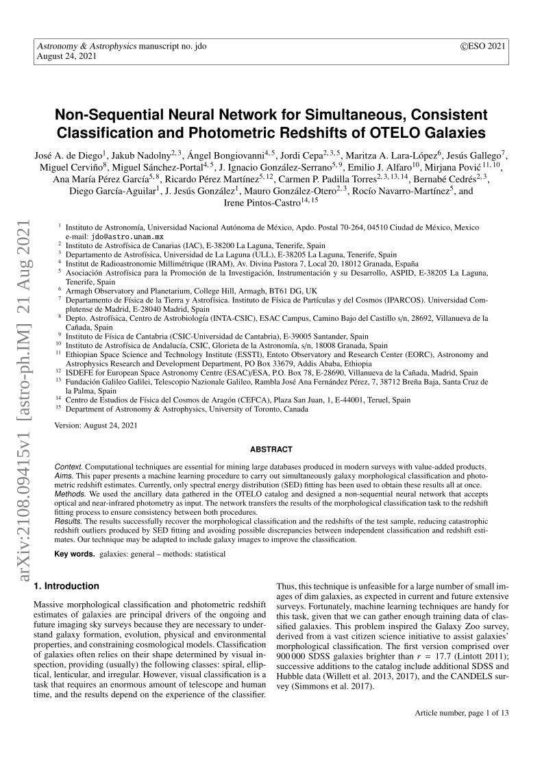
Table 4. Misclassified galaxies.

ID Visual OTELO DNN z_.spec. z_.OTELO. z_.DNN.26 ET LT 0.75 0.62 0.79

1482 LT LT ET 0.53 0.68 0.561483 LT ET LT 1.02 0.83 0.992170 LT LT ET 0.68 0.82 0.715229 LT ET 1.15 0.85 0.986176 LT ET LT 0.32 0.25 0.42

( pLT = 0.92) dominates over the ET galaxies (( pET = 0.08), as-signing all the galaxies to the LT class yields a baseline accuracyof 0.92 Table 3 shows the contingency table for the classificationresults. From the 31 ET and 339 LT OTELO galaxies, the DNNrecovers 28 and 336, respectively. Three ET and three LT galax-ies are mismatched. The accuracy attained by the neural networkcan be inferred from this table, resulting in 0.984 ± 0.007. Thisaccuracy represents a considerable improvement compared withthe classification baseline of 0.92. Similarly, the True LT Rateand the True ET Rate can be gathered from this table, resultingin 0.991 ± 0.006 and 0.90 ± 0.06, respectively. The accuracy ob-tained with our non-sequential model using just photometric datamatches our previous result reported in de Diego et al. (2020,0.985 ± 0.007), where we also included the Sérsic index.

Table 4 presents the results for the objects with discrepantclassifications. Column 1 in this table shows the OTELO iden-tifier. Columns 2, 3, and 4 indicate the visual classification per-formed by the authors, OTELO, and the neural network classi-fications. Finally, columns 5, 6, and 7 show the spectroscopicredshift, the OTELO, and the neural network estimates. OTELOemploys 4 Coleman et al. (1980) Hubble-type and 6 Kinney et al.(1996) starburst templates for the LePhare tool SED fitting. TheHubble-type templates used are, from earlier to later types, ellip-ticals (E), spirals (Sbc and Scd), and irregular (Im) galaxies. Wenote that all the discrepant classifications were a better fit withthe Hubble templates E and Sbc.

Figure 3 shows the HST Advanced Camera Survey (ACS)F814W images of these misclassified galaxies, but the imagefor ID 00026 is not available. The galaxy SEDs are presentedin Fig. 4. Galaxy ID 05229 is actually a mixed group of unre-solved galaxies in the GTC-OTELO low-resolution image. Thisobject is a bright infrared and X-ray source (Georgakakis et al.2010, source irx-8), and OTELO galaxy templates poorly fitthe observed SED, probably because the dominant object in theimage may be an obscured AGN (Zheng et al. 2004, sourceCFRS-14.1157). The spectral redshift reported by Matthewset al. (2013) is 1.14825, but Zheng et al. (2004) find a red-shift of 1.0106 that is in better agreement with both the SEDfitting (0.85) and the neural network prediction (0.98). The otherfour galaxies are all visually classified as LT. Briefly, the visualand OTELO’s classifications agree for galaxies ID 001482 andID 02170, but not for galaxies ID 01483 and ID 06176, for whichthe visual matches the DNN classification.

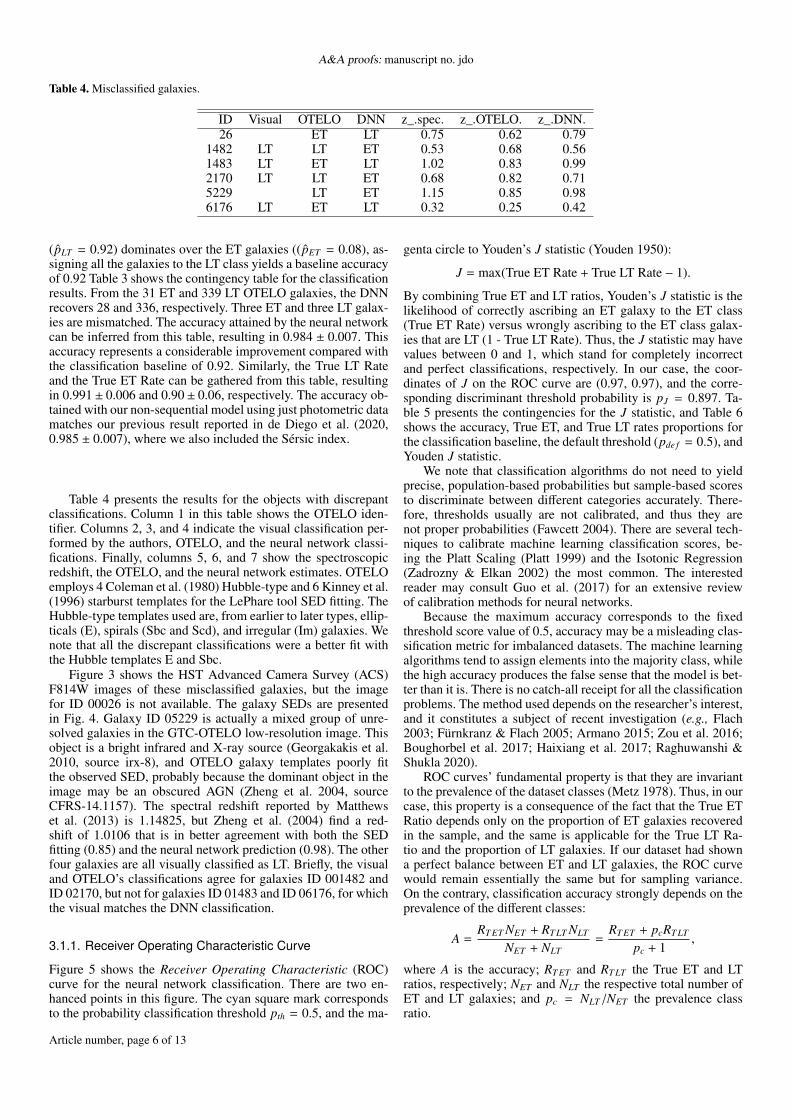
3.1.1. Receiver Operating Characteristic Curve

Figure 5 shows the Receiver Operating Characteristic (ROC)curve for the neural network classification. There are two en-hanced points in this figure. The cyan square mark correspondsto the probability classification threshold pth = 0.5, and the ma-

genta circle to Youden’s J statistic (Youden 1950):

J = max(True ET Rate + True LT Rate − 1).

By combining True ET and LT ratios, Youden’s J statistic is thelikelihood of correctly ascribing an ET galaxy to the ET class(True ET Rate) versus wrongly ascribing to the ET class galax-ies that are LT (1 - True LT Rate). Thus, the J statistic may havevalues between 0 and 1, which stand for completely incorrectand perfect classifications, respectively. In our case, the coor-dinates of J on the ROC curve are (0.97, 0.97), and the corre-sponding discriminant threshold probability is pJ = 0.897. Ta-ble 5 presents the contingencies for the J statistic, and Table 6shows the accuracy, True ET, and True LT rates proportions forthe classification baseline, the default threshold (pde f = 0.5), andYouden J statistic.

We note that classification algorithms do not need to yieldprecise, population-based probabilities but sample-based scoresto discriminate between different categories accurately. There-fore, thresholds usually are not calibrated, and thus they arenot proper probabilities (Fawcett 2004). There are several tech-niques to calibrate machine learning classification scores, be-ing the Platt Scaling (Platt 1999) and the Isotonic Regression(Zadrozny & Elkan 2002) the most common. The interestedreader may consult Guo et al. (2017) for an extensive reviewof calibration methods for neural networks.

Because the maximum accuracy corresponds to the fixedthreshold score value of 0.5, accuracy may be a misleading clas-sification metric for imbalanced datasets. The machine learningalgorithms tend to assign elements into the majority class, whilethe high accuracy produces the false sense that the model is bet-ter than it is. There is no catch-all receipt for all the classificationproblems. The method used depends on the researcher’s interest,and it constitutes a subject of recent investigation (e.g., Flach2003; Fürnkranz & Flach 2005; Armano 2015; Zou et al. 2016;Boughorbel et al. 2017; Haixiang et al. 2017; Raghuwanshi &Shukla 2020).

ROC curves’ fundamental property is that they are invariantto the prevalence of the dataset classes (Metz 1978). Thus, in ourcase, this property is a consequence of the fact that the True ETRatio depends only on the proportion of ET galaxies recoveredin the sample, and the same is applicable for the True LT Ra-tio and the proportion of LT galaxies. If our dataset had showna perfect balance between ET and LT galaxies, the ROC curvewould remain essentially the same but for sampling variance.On the contrary, classification accuracy strongly depends on theprevalence of the different classes:

A =RT ET NET + RT LT NLT

NET + NLT=

RT ET + pcRT LT

pc + 1,

where A is the accuracy; RT ET and RT LT the True ET and LTratios, respectively; NET and NLT the respective total number ofET and LT galaxies; and pc = NLT /NET the prevalence classratio.

Article number, page 6 of 13

José A. de Diego et al.: Non-sequential Neural Network for OTELO Galaxies

ID 00026 ID 01482

HST imagenot available

ID 01483 ID 02170

ID 05229 ID 06176

Fig. 3. Hubble Space Telescope F814W images for galaxies with discrepant classification. The OTELO ID 00026 galaxy image is not availablefrom the AEGIS HST-ACS image archive (Davis et al. 2007). The left axis corresponds to relative declination in arcsec. The bottom axis indicatesthe relative right ascension in arcsec.

Figure 5 shows the iso-accuracy lines for both a theoreticallybalanced dataset (red lines) and our imbalanced sample (in gray).The iso-accuracy lines for the balanced data intersect the ROCcurve at two points with inverted but approximately equal True

LT Rate and True ET Rate values. However, the iso-accuracylines for the imbalanced data intersect the ROC curve at signif-icantly different values. For example, the baseline iso-accuracyedge —orange line— intersects the curve at (1,0) and approxi-

Article number, page 7 of 13

A&A proofs: manuscript no. jdo

µm

log(

Fν µ

Jy)

1 10

0

1

2ID 00026

µm

log(

Fν µ

Jy)

1 10

−1

0

1

ID 01482

µm

log(

Fν µ

Jy)

1 10

−1

0

1

ID 01483

µm

log(

Fν µ

Jy)

1 10

0

1

2

ID 02170

µm

log(

Fν µ

Jy)

1 10

0

1

2

3 ID 05229

µm

log(

Fν µ

Jy)

1 10

1

2

ID 06176

Fig. 4. Spectral energy distributions for galaxies with discrepant classification. The solid blue line indicates the best-fitting OTELO template.

mately (0.91, 0.96). The high dependence of the True ET Rate(but not the True LT Rate) on the accuracy is a non-desired con-sequence of our highly imbalanced data.

The difference between the True LT and ET rates associatedwith our network’s maximum accuracy at the probability thresh-old of 0.5 reveals that we are misclassifying a larger proportion

Article number, page 8 of 13

José A. de Diego et al.: Non-sequential Neural Network for OTELO Galaxies

1.0 0.8 0.6 0.4 0.2 0.0

0.0

0.2

0.4

0.6

0.8

1.0

True LT Rate

True

ET

Rat

e

0.9

0.8

0.7

0.6

0.5

0.4

0.3

0.2

0.1

Fig. 5. Receiver Operating Characteristic (ROC) curve for galaxy clas-sification. For clarity, the specificity and sensitivity axes, common instatistical studies, have been renamed as True LT Rate and True ETRate, respectively. The stepped black line is the ROC curve obtainedwith the neural network. The ascending diagonal red lines show theiso-accuracy edges for a balanced sample of ET and LT galaxies. Sim-ilarly, the gray dotted lines represent the iso-accuracy fringes for ourimbalanced sample. Iso-accuracy lines of the same value intersect atthe descending diagonal black dotted line. The orange iso-accuracy linepassing through coordinates (1,0) corresponds to the baseline. The cyansquare mark indicates the True LT and ET Rates obtained through themaximum accuracy criterium (0.991 and 0.90, respectively). The ma-genta circle indicates the rates obtained from Youden’s J statistic (0.97for both the True LT and ET Rates).

of ET than LT galaxies (see Fig. 5). For maximum accuracy, thenumber of misclassified objects is similar for both galaxy types(in this case, it is the same by chance), as shown in Table 3. How-ever, if we apply our trained network and the 0.5 thresholds toanother sample consisting of a different proportion of ET and LTgalaxies, we will obtain similar proportions of misclassified ob-jects, but we will not attain the same accuracy the model achievesin the current sample. It is well known that ET and LT galaxiesdo not distribute the same in different environments (e.g., Calviet al. 2012) and present opposite distribution gradients in clusters(e.g., Doi et al. 1995).

If the accuracy varies depending on the sample characteris-tics, it is not the best choice for deciding the probability thresh-old for classification. Youden’s J statistic provides well-balancedTrue LT and ET rates that will deliver comparable results no mat-ter the class prevalences in the sample.

3.2. Photometric redshifts

Bongiovanni et al. (2019) fitted LePhare templates to multifre-quency broadband data to estimate photometric redshifts in theOTELO catalog, achieving a precision of ∆z ∼ 0.2, which is typ-ical for this kind of estimates. Previous studies have shown thatneural networks often provide better assessments than SED fit-ting (Firth et al. 2003; Tagliaferri et al. 2003; Singal et al. 2011;Brescia et al. 2014; Eriksen et al. 2020). For galaxies at z . 0.4errors are ∆zphot ' 0.02 (Firth et al. 2003; Tagliaferri et al. 2003;

Table 5. Contingency table using Youden’s J statistic threshold.

ETOTELO LTOTELO SumETDNN 30 11 41LTDNN 1 328 329

Sum 31 339 370

Table 6. Classification statistics

Classifier Accuracy True ET Rate True LT RateBaseline 0.92± 0.02 0 1Default Th. 0.984± 0.007 0.90± 0.06 0.991± 0.006Youden’s J 0.97± 0.01 0.97± 0.04 0.97± 0.01

Brescia et al. 2014) even using a small database of 155 galaxiesfor training and 44 for testing (Vanzella et al. 2004). Errors in-crease as the samples extend to redshifts z & 1 (Firth et al. 2003;Tagliaferri et al. 2003) reaching values of ∆z ' 0.1 (Vanzellaet al. 2004), and decrease as the number of available photometricbands gets larger, as for the 40 narrow bands sample of Eriksenet al. (2020). Besides the photometric data, some authors haveprovided morphological information to improve the neural net-work’s redshift estimates, with inconclusive results. Thus, Sin-gal et al. (2011) and Wilson et al. (2020) report that including,in addition to the photometry, several shape parameters such asthe concentration, Sérsic index, the effective radius, or the ellip-ticity, do not produce any improvement in the redshift estimate.In contrast, Tagliaferri et al. (2003) include photometry, surfacebrightnesses, and Petrosian radii and fluxes, reducing the errorsby a factor of about 30%. More recently, Menou (2019) presentsa non-sequential network with two inputs and one output, a con-volutional branch to analyze images, and a branch composed of adense set of layers to deal with the photometric data, reporting animprovement in the redshift estimates. For our redshift analysis,we take into account the probability yielded by the Classificationmodule.

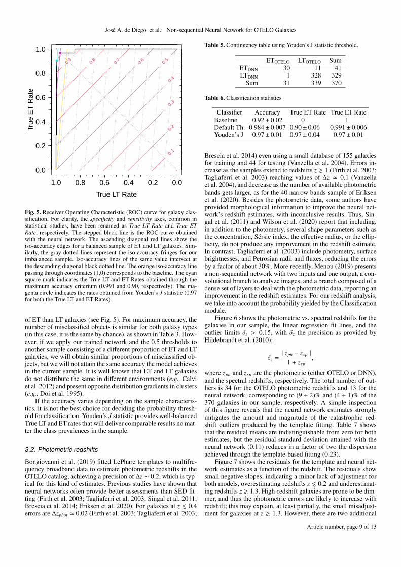
Figure 6 shows the photometric vs. spectral redshifts for thegalaxies in our sample, the linear regression fit lines, and theoutlier limits δz > 0.15, with δz the precision as provided byHildebrandt et al. (2010):

δz =| zph − zsp |

1 + zsp,

where zph and zsp are the photometric (either OTELO or DNN),and the spectral redshifts, respectively. The total number of out-liers is 34 for the OTELO photometric redshifts and 13 for theneural network, corresponding to (9 ± 2)% and (4 ± 1)% of the370 galaxies in our sample, respectively. A simple inspectionof this figure reveals that the neural network estimates stronglymitigates the amount and magnitude of the catastrophic red-shift outliers produced by the template fitting. Table 7 showsthat the residual means are indistinguishable from zero for bothestimates, but the residual standard deviation attained with theneural network (0.11) reduces in a factor of two the dispersionachieved through the template-based fitting (0.23).

Figure 7 shows the residuals for the template and neural net-work estimates as a function of the redshift. The residuals showsmall negative slopes, indicating a minor lack of adjustment forboth models, overestimating redshifts z . 0.2 and underestimat-ing redshifts z & 1.3. High-redshift galaxies are prone to be dim-mer, and thus the photometric errors are likely to increase withredshift; this may explain, at least partially, the small misadjust-ment for galaxies at z & 1.3. However, there are two additional

Article number, page 9 of 13

A&A proofs: manuscript no. jdoHildebrandt et al. 2010 ... Outliers

zspec

z pho

t

0.0 0.2 0.4 0.6 0.8 1.0 1.2 1.4

0

1

2

3

Fig. 6. Photometric vs. spectroscopic redshift comparison. Gray crossesindicate the OTELO template fitting photometric redshifts and filled redcircles the neural network estimates. The regression lines for the dif-ferent fits —not plotted— are barely distinguishable from the perfectcorrelation between photometric and spectroscopic redshifts (blue-solidthick line). The blue-dashed thin lines show the Hildebrandt et al. (2010)outlier limits.

causes in the neural network that may contribute to this lack offitting. The first one is that neural networks are interpolatingapproximation functions; at low-redshifts, the predicted valuesmust be larger than zero, and at high-redshifts less than 1.4 be-cause these are the constraints in the training sample range ofredshifts. The second cause is associated with the small numberof galaxies at low and high-redshifts shown in Fig. 1. Thus, be-cause of the insufficient number of subjects in the training sam-ple, the network tends to push the redshift estimates towards themost populated redshift areas, increasing low-redshift and de-creasing high-redshift estimates.

The standard deviation of our sample residuals, σz = 0.11,improves the redshift accuracy obtain Vanzella et al. (2004) fortheir spectroscopic redshift sample (σz = 0.14) using 150 Hub-ble Deep Field North galaxies for training and 34 Hubble DeepField South objects at z < 2 for validation. Also the median pre-cision δz = 0.040 ± 0.002 improves Vanzella et al. δz = 0.06results significantly. Comparing our results with other studies isless straightforward because of the large number of galaxies in-volved and the redshift’s reduced range. For example, Bresciaet al. (2014) used a sample of 497 339 Sloan galaxies at z < 1,of which 90% were at z < 0.345 and with a distribution peakat z ≈ 0.1. In contrast, only 13% of our sample is located atz < 0.345, and the distribution peaks at z ≈ 0.8 (see Fig. 1).

3.3. Effect of the classification on the redshift estimate

The galaxy colors are related to both the redshift and the mor-phology. However, the contradictory results obtained by otherresearchers for and against including morphological data to in-crease the redshift estimate accuracy (Tagliaferri et al. 2003; Sin-gal et al. 2011; Menou 2019; Wilson et al. 2020) suggest thatthe morphological properties provide limited information to at-tain this goal. Therefore, we used bootstrap resampling to ana-lyze the effect of the galaxy classification probabilities passed onthe redshift module in our neural network model. We consideredthat dropouts suppress a fraction of the layer outputs but do notchange neurons’ weights, which are continually updated duringtraining. Therefore, the concatenate layer in our model has 513inputs and their corresponding weights; 512 of these inputs cor-respond to the outputs from the Base module, regardless of this

Table 7. Redshift residuals.

OTELO DNNMean 0.00± 0.02 0.00± 0.03Sd. Dev. 0.23± 0.06 0.11± 0.02Intercept 0.11± 0.04 0.10± 0.02Slope -0.16± 0.04. -0.15± 0.02

module dropout, and only one linked to the Classification mod-ule output. In addition, the concatenate layer has its own weights.

Because of the indeterministic nature of the neural networks,hidden layer neurons estimate different relations in each trainingrun. Consequently, the weights will differ from one bootstraprun to another, and only a few in each run will show an abso-lute value large enough to contribute to the result significantly.Thus, monitoring a single random weight during different runswill reproduce the layer weight distribution. The only exceptionmay be the weight that is always associated with the output ofthe classification module if this factor has some effect on theconcatenate layer outcome. In this case, we expect an absolutelarger weight and possibly a different weight distribution shape.

We have performed 1000 bootstrap training runs with the fi-nal architecture to analyze the weight distribution of the con-catenate layer and the neuron associated with the classificationoutput in this layer. We used all the galaxies from our sam-ple as the training set for these runs (neither validation nor testsets were necessary for this task). Figure 8 shows the quantile-quantile (Q-Q) plots for the weights of the whole concatenatelayer, a randomly chosen neuron, and the neuron linked to theclassification module output. In the case of the whole concate-nate layer, we extracted the weights from a single run; the shapeof the distribution does not change from run to run. For easycomparison with the other distributions presented in the figure,we have standardized them all by subtracting the mean and di-viding by the standard deviation of the layer weights; for indi-vidual neurons, we standardized each weight using the layer dis-tribution statistics corresponding to each bootstrap run. We notethat the distribution of the concatenate layer weights (solid blueline in Fig. 8) presents a normal-like distribution (dashed redline). As expected, the distribution of the bootstrap runs of a ran-domly selected neuron in this layer (solid yellow line) closelymirrors the distribution of the whole layer. However, the distri-bution of the bootstrap runs of the neuron associated with theoutput of the classification layer (gray solid line) is quite differ-ent. It contrasts with the normal distribution due to its upwardsshift that indicates a central value different from zero (medianof 0.66 ± 0.05), and its appearance evinced by the S-shaped linethat corresponds to a thin tailed or platykurtic distribution withkurtosis of 1.81±0.04. Platykurtic distributions and medians arerobust to the presence of outliers, and thus the different behaviorof the classification neuron cannot be ascribed to a few extremeneuron weights. For comparison, the random neuron weightsshow statistics more similar to the normal distribution, with amedian of 0.11 ± 0.04 and kurtosis of 3.1 ± 0.2.

In total, 41% and 13% of the classification neuron weightsare greater than 1σ and 2σ, respectively. These results con-trast with those for the random neuron and the concatenate layerweights, both with 15% and 1% performance at these sigma val-ues. However, even if the differences are notable, there is a ratherlarge probability that the classification neuron does not signifi-cantly affect the redshift estimate for a single training. This be-havior may be a consequence of the limited training due to oursample’s small number of objects. Regardless of a definitive ex-

Article number, page 10 of 13

José A. de Diego et al.: Non-sequential Neural Network for OTELO Galaxies

+ ++++

+

+

+++

+ ++ + + ++

+++

+++

++ ++ ++

++ + ++ +++

++

+++ +++

+ ++ ++

+++ ++

+

+ ++ + ++ + ++

+++

+ +++++ ++++

+ ++

+ ++ ++ ++ ++++

+

++ ++ +++ +

+

+ +

+

+

++++ +

+

+ +++ + +

++

++

+

++

+

+ ++ + ++ +

+++ +

++

+++

+

+

++

++

+

+

+ ++

+

+ ++ ++

+ ++ ++++++ + +

++

++ ++

+++

+ ++ ++++ + + ++ ++ ++ ++ ++++

+ +++

++ + ++ ++ ++ ++ + ++

+

++ +++ +++

++ ++++ +++ ++++ ++ +++++ + +

+++++ + ++++ ++++ + ++ + +

++ + +++ ++ ++ ++

++ ++ ++ ++

+++ ++ ++ +

+++ +

++ +++ +

++ ++

+++

++ + + ++ + ++++

+++ + ++ +++ + +

++ +++

+

+++ ++++ ++ + ++ + +

+++

++++

++ +++

+ + +

x

Tem

plat

e

0

1

2

+ ++++

+

+++ ++ ++ + +++ ++++ ++++

++ ++

+

++ ++ +++

++ +++ ++++ ++ ++ +++ ++ ++ ++ + ++ + ++++ ++ +++++ ++++ + + ++ ++ ++ ++ +++ ++

++ ++

+++ + ++ + + +++++ +++ +++

+ + ++

+ ++++ ++ ++

+++ ++++ + +

+++ ++

++++ +

+++ +++

+ ++ +++ ++ ++++++ + ++ + ++ ++++ ++ ++

++++ + + ++ +

+ ++ +

+ + ++++ ++

+++ +++ ++ ++ ++ + ++ +

++ +++ ++ +++ ++ ++ +++ ++++ ++ +++++ + ++ ++++ +

++++

++++ + ++ + +++ + +++ ++ ++ ++ ++ ++ ++ +++ ++ ++ ++ + +++ ++ + +++ + ++ ++ ++ +++ + + ++ + +

++ +++

+ + ++ + ++ + +++ +++ + +++ ++++ ++ + ++ + ++ ++++ ++++ ++++ + +

zspec

Net

wor

k

0.0 0.2 0.4 0.6 0.8 1.0 1.2 1.4−1

0

1

Fig. 7. Photometric redshift residuals. Obtained from LePhare templatefittings (upper panel) and neural network predictions (lower panel). Theresiduals are plotted as plus signs, the regression fit as a thick green solidline. Dashed blue lines indicate 99% confidence bands and pointed redlines the 99% prediction bands.

planation, whether or not the weight is large enough to influencethe redshift estimate may explain the disagreement between theresults obtained by the different groups that have included mor-phological parameters in their neural networks for photometricestimates of the redshift.

Our analysis using a non-sequential neural network modelhas shown that it is feasible to incorporate morphological clas-sification to estimate galaxies’ redshifts. It is worth noting thatwe have used galaxy photometry as it is, without extinctions andk-corrections that would incorporate theoretical models into apure empirical methodology. The number of OTELO galaxieswith spectroscopically measured redshifts (370) is rather smallfor neural network training. However, we have obtained classifi-cation and photometric redshift accuracies that compete with andimprove those obtained through SED template fitting. The red-shift range of the OTELO spectroscopic sample ends at z ' 1.4,just at the beginning of the redshift desert (1.4 < z < 3). Futurework should cover this and higher redshift regions where ob-taining bulk spectroscopic measurements has been challenginguntil the recent development of near-infrared multi-object spec-trographs (e.g.,MOSFIRE McLean et al. 2010, 2012).

These results show that non-sequential neural networks canproduce several outcomes simultaneously. By sharing repeatedcalculations between the fitting procedures, the computing andtraining total times reduce by a factor that depends on the com-plexity of the procedure and shared intermediate byproducts.Moreover, transferring results between procedures ensures theinternal consistency of the predictions.

4. Conclusions

The first methods for automatically analyzing galaxy surveysrelied on the SED fitting of observed or simulated spectra.These methods allow simultaneous morphological classifica-tion and photometric redshift estimates of the sources at theexpense of many catastrophic mismatches. Machine-learning-based models —support vector machines, random forest, andneural networks— are becoming more and more popular foranalyzing survey data, and they have shown to be more robustthan SED fitting for redshift estimates. The interest in neuralnetworks has increased spectacularly during the last five years,fuelled by advances in hardware and tensor-oriented libraries.

−3 −2 −1 0 1 2 3

z−scores

Sta

ndar

dize

d W

eigh

ts

−3

−2

−1

0

1

2

3

Fig. 8. Q-Q plot of the weights of the concatenate layer. The solid blueline shows the standardized distribution of the 513 concatenate layerweights obtained in a single training. The solid gray line displays thestandardized distribution of the weights corresponding to the neuronlinked to the output of the Classification module, obtained from 1000bootstrap runs. The blue line shows the standardized distribution of thebootstrap runs for a random neuron weight. The red dashed line indi-cates the expected relation for a standard normal distribution.

Some advantages over other machine learning techniques arethat neural networks efficiently deal with missing data and feedgalaxy images directly into the model. However, machine learn-ing morphological classification and photometric redshift esti-mates have been computed independently with different models.This split in the machine learning methods may produce incon-sistencies due to the tendency to level low-redshift ET and high-redshift LT galaxy colors.

This study tested a non-sequential neural network architec-ture for simultaneous galaxy morphological SED-based classi-fication and photometric redshift estimates, using optical andnear-infrared photometry of the 370 sources with spectroscopicredshift listed in the OTELO survey. These photometric datawere not subjected to extinction or k-corrections. We found thatour non-sequential neural network provides accurate classifica-tion and precise photometric redshift estimates. Besides, sharingthe classification results tends to improve the redshift estimatesand the congruence of the predictions. Our results demonstratethe non-sequential neural networks’ capabilities to deal with sev-eral problems simultaneously and share intermediate results be-tween the network modules. Furthermore, the analysis of theneuron weights shows that including the morphological classi-fication prediction often improves the photometric redshift esti-mate.

We have used a ROC curve and the Youden J statistic to ob-tain a classification threshold that provides a better equilibriumbetween misclassified galaxy types and reduces the problem ofimbalanced samples. Besides, our neural network reduces themean error of the photometric redshift estimates by a factor oftwo relative to the SED template fitting.

This study strongly suggests that the benefits gained by si-multaneously treating morphological classification and photo-metric redshift estimates may also address other prediction prob-lems across a wide range of astronomical problems, particularlywhen consistency between the results is required. Most notably,this is the first study to our knowledge that provides simulta-

Article number, page 11 of 13

A&A proofs: manuscript no. jdo

neous and consistent predictions using a single deep learningmethodology, a non-sequential neural network model.

The OTELO sample has some limitations that are worthnoting. The first one is the low number of sources with mea-sured spectral redshifts; machine learning methods perform bet-ter with many available training data. Besides, the scarcity ofspectral redshift measurements for low (z < 0.2) and high-redshift (z > 1.3) sources limits the precision of the estimatesat these redshift ranges. The last limitation is the redshift cut-offat z ≈ 1.4 that restricts the range of our study.

Currently, the OTELO project is conducting spectroscopicalmonitoring for about two hundred new objects using the OSIRISMOS instrument attached at the GTC. These observations willadd certainty about the nature and the redshifts of Hβ, Hα, [OIII],and HeII emitter candidates, as well as compact early ellipticalgalaxies. In addition, the results will be compared with estimatesobtained from our network.

Future work should include a large and redshift balancedsample of galaxies and extend the redshift range to cover all ob-servable sources with modern instruments. For resolved galax-ies, models allowing both images and tabulated data —multi-input non-sequential neural networks— can benefit from multi-band photometry and morphological profile aspects for betterclassification. In particular, the photometry of spiral galaxies de-pends on their orientation, changing the relative contribution ofdisk and bulge components. Thus, galaxy classification will ben-efit from the support of images that may disentangle orientationeffects.

Acknowledgements. The authors gratefully thank the anonymous referee for theconstructive comments and recommendations, which helped improve the paper’sreadability and quality.This work was supported by the project Evolution of Galaxies, of referenceAYA2014-58861-C3-1-P and AYA2017-88007-C3-1-P, within the "Programa es-tatal de fomento de la investigación científica y técnica de excelencia del PlanEstatal de Investigación Científica y Técnica y de Innovación (2013-2016)" ofthe "Agencia Estatal de Investigación del Ministerio de Ciencia, Innovación yUniversidades", and co-financed by the FEDER "Fondo Europeo de DesarrolloRegional".JAD is grateful for the support from the UNAM-DGAPA-PASPA 2019 program,the UNAM-CIC, the Canary Islands CIE: Tricontinental Atlantic Campus 2017,and the kind hospitality of the IAC.MP acknowledges financial supports from the Ethiopian Space Science andTechnology Institute (ESSTI) under the Ethiopian Ministry of Innovation andTechnology (MoIT), and from the Spanish Ministry of Economy and Com-petitiveness (MINECO) through projects AYA2013-42227-P and AYA2016-76682C3-1-P, and from the Spanish Ministerio de Ciencia e Innovación -Agencia Estatal de Investigación through projects PID2019-106027GB-C41 andAYA2016-76682C3-1-P.APG, MSP and RPM were supported by the PNAYA project: AYA2017–88007–C3–2–P.JG was supported by the PNAYA project AYA2018–RTI-096188-B-i00.MC & APG are also funded by Spanish State Research Agency grant MDM-2017-0737 (Unidad de Excelencia María de Maeztu CAB).JIGS receives support through the Proyecto Puente 52.JU25.64661 (2018)funded by Sodercan S.A. and the Universidad de Cantabria, and PGC2018–099705–B–100 funded by the Ministerio de Ciencia, Innovación y Universi-dades.EJA acknowledges funding from the State Agency for Research of the SpanishMCIU through the “Center of Excellence Severo Ochoa" award to the Instituto deAstrofísica de Andalucía (SEV-2017-0709) and from grant PGC2018-095049-B-C21.Based on observations made with the Gran Telescopio Canarias (GTC), installedin the Spanish Observatorio del Roque de los Muchachos of the Instituto de As-trofísica de Canarias, in the island of La Palma. This work is (partly) based ondata obtained with the instrument OSIRIS, built by a Consortium led by the Insti-tuto de Astrofísica de Canarias in collaboration with the Instituto de Astronomíaof the Universidad Autónoma de México. OSIRIS was funded by GRANTECANand the National Plan of Astronomy and Astrophysics of the Spanish Govern-ment.

ReferencesAmado, Z. B., Povic, M., Sánchez-Portal, M., et al. 2019, MNRAS, 485, 1528Armano, G. 2015, Information Sciences, 325, 466Arnouts, S., Cristiani, S., Moscardini, L., et al. 1999, MNRAS, 310, 540Banerji, M., Lahav, O., Lintott, C. J., et al. 2010, MNRAS, 406, 342Benítez, N., Moles, M., Aguerri, J. A. L., et al. 2009, ApJ, 692, L5Bom, C. R., Makler, M., Albuquerque, M. P., & Brandt, C. H. 2017, A&A, 597,

A135Bongiovanni, A., Ramón-Pérez, M., Pérez García, A. M., et al. 2019, A&A, 631,

A9Boughorbel, S., Jarray, F., & El-Anbari, M. 2017, PLOS ONE, 12, e0177678Brescia, M., Cavuoti, S., Longo, G., & De Stefano, V. 2014, A&A, 568Bruzual, G. & Charlot, S. 2003, MNRAS, 344, 1000Calvi, R., Poggianti, B. M., Fasano, G., & Vulcani, B. 2012, MNRAS, 419, L14Carrasco Kind, M. & Brunner, R. J. 2013, MNRAS, 432, 1483Chollet, F. 2017, Deep learning with Python (Manning Publications Co.)Chollet, F. & Allaire, J. J. 2017, Deep learning with R (Manning Publications

Co.)Coleman, G. D., Wu, C.-C., & Weedman, D. W. 1980, The Astrophysical Journal

Supplement Series, 43, 393Cunha, C. E., Huterer, D., Lin, H., Busha, M. T., & Wechsler, R. H. 2014, MN-

RAS, 444, 129Cybenko, G. 1989, Mathematics of control, signals and systems, 2, 303Davis, M., Guhathakurta, P., Konidaris, N. P., et al. 2007, ApJ, 660, L1de Diego, J. A., Nadolny, J., Bongiovanni, A., et al. 2020, A&A, 638, A134Deng, J., Dong, W., Socher, R., et al. 2009, in 2009 IEEE conference on computer

vision and pattern recognition (Ieee), 248–255Deng, X.-F. 2013, Research in Astronomy and Astrophysics, 13, 651Dieleman, S., Willett, K. W., & Dambre, J. 2015, MNRAS, 450, 1441Doi, M., Fukugita, M., Okamura, S., & Turner, E. L. 1995, AJ, 109, 1490Domínguez Sánchez, H., Huertas-Company, M., Bernardi, M., Tuccillo, D., &

Fischer, J. L. 2018, MNRAS, 476, 3661Eriksen, M., Alarcon, A., Cabayol, L., et al. 2020, arXiv e-prints,

arXiv:2004.07979Fawcett, T. 2004, MLear, 31, 1Firth, A. E., Lahav, O., & Somerville, R. S. 2003, MNRAS, 339, 1195Flach, P. A. 2003, in Twentieth International Conference on Machine Learning

(ICML-2003) (AAAI Press)Fürnkranz, J. & Flach, P. A. 2005, MLear, 58, 39Georgakakis, A., Rowan-Robinson, M., Nandra, K., et al. 2010, MNRAS, 406,

420Guo, C., Pleiss, G., Sun, Y., & Weinberger, K. Q. 2017, arXiv preprint

arXiv:1706.04599Haixiang, G., Yijing, L., Shang, J., et al. 2017, Expert Systems with Applications,

73, 220Hildebrandt, H., Arnouts, S., Capak, P., et al. 2010, A&A, 523, A31Hornik, K. 1991, NN, 4, 251Huertas-Company, M., Rouan, D., Tasca, L., Soucail, G., & Le Fèvre, O. 2008,

A&A, 478, 971Ilbert, O., Arnouts, S., McCracken, H. J., et al. 2006, A&A, 457, 841Ilbert, O., Capak, P., Salvato, M., et al. 2009, ApJ, 690, 1236James, G., Witten, D., Hastie, T., & Tibshirani, R. 2013, An introduction to statis-

tical learning : with applications in R, Springer texts in statistics, (New York:Springer), xvi, 426 pages

Jones, E. & Singal, J. 2017, A&A, 600, A113Khramtsov, V., Akhmetov, V., & Fedorov, P. 2020, A&A, 644, A69Kinney, A. L., Calzetti, D., Bohlin, R. C., et al. 1996, The Astrophysical Journal,

467, 38Leshno, M., Lin, V. Y., Pinkus, A., & Schocken, S. 1993, NN, 6, 861Lintott, C. e. a. 2011, MNRAS, 410, 166Marmanis, D., Datcu, M., Esch, T., & Stilla, U. 2015, IEEE Geoscience and

Remote Sensing Letters, 13, 105Matthews, D. J., Newman, J. A., Coil, A. L., Cooper, M. C., & Gwyn, S. D. J.

2013, ApJS, 204, 21McLean, I. S., Steidel, C. C., Epps, H., et al. 2010, in Ground-based and Air-

borne Instrumentation for Astronomy III, Vol. 7735 (International Society forOptics and Photonics), 77351E

McLean, I. S., Steidel, C. C., Epps, H. W., et al. 2012, in Ground-based andAirborne Instrumentation for Astronomy IV, Vol. 8446 (International Societyfor Optics and Photonics), 84460J

Menou, K. 2019, MNRAS, 489, 4802Metz, C. 1978, Seminars in nuclear medicine, 8 4, 283Mucesh, S., Hartley, W. G., Palmese, A., et al. 2021, MNRAS, 502, 2770Nadolny, J., Bongiovanni, A., Cepa, J., et al. 2021, A&A, 647, A89Newman, J. A., Cooper, M. C., Davis, M., et al. 2013, ApJS, 208, 5Odewahn, S. C., Windhorst, R. A., Driver, S. P., & Keel, W. C. 1996, ApJ, 472,

L13Padilla, C., Castander, F. J., Alarcón, A., et al. 2019, AJ, 157, 246Pintos-Castro, I., Povic, M., Sánchez-Portal, M., et al. 2016, A&A, 592, A108

Article number, page 12 of 13

José A. de Diego et al.: Non-sequential Neural Network for OTELO Galaxies

Platt, J. 1999, Advances in large margin classifiers, 10, 61Pourrahmani, M., Nayyeri, H., & Cooray, A. 2018, ApJ, 856, 68Povic, M., Huertas-Company, M., Aguerri, J. A. L., et al. 2013, MNRAS, 435,

3444Povic, M., Márquez, I., Masegosa, J., et al. 2015, MNRAS, 453, 1644Povic, M., Sánchez-Portal, M., Pérez García, A. M., et al. 2012, A&A, 541, A118Raghu, M., Zhang, C., Kleinberg, J., & Bengio, S. 2019, in Advances in Neural

Information Processing Systems, ed. H. Wallach, H. Larochelle, A. Beygelz-imer, F. d'Alché-Buc, E. Fox, & R. Garnett, Vol. 32 (Curran Associates, Inc.),3347–3357

Raghuwanshi, B. S. & Shukla, S. 2020, Knowledge-Based Systems, 187, 104814Raihan, S. F., Schrabback, T., Hildebrandt, H., Applegate, D., & Mahler, G. 2020,

MNRAS, 497, 1404Salvato, M., Ilbert, O., & Hoyle, B. 2019, Nature Astronomy, 3, 212Serra-Ricart, M., Calbet, X., Garrido, L., & Gaitan, V. 1993, AJ, 106, 1685Serra-Ricart, M., Gaitan, V., Garrido, L., & Perez-Fournon, I. 1996, A&AS, 115,

195Simmons, B. D., Lintott, C., Willett, K. W., et al. 2017, MNRAS, 464, 4420Singal, J., Shmakova, M., Gerke, B., Griffith, R. L., & Lotz, J. 2011, PASP, 123,

615Strateva, I. e. a. 2001, The Astronomical Journal, 122, 1861

Tagliaferri, R., Longo, G., Andreon, S., et al. 2003, Neural Networks for Photo-metric Redshifts Evaluation, Vol. 2859 (Lecture Notes in Computer Science),226–234

Tuccillo, D., González-Serrano, J. I., & Benn, C. R. 2015, MNRAS, 449, 2818Tuccillo, D., Huertas-Company, M., Decencière, E., et al. 2018, MNRAS, 475,

894Vanzella, E., Cristiani, S., Fontana, A., et al. 2004, A&A, 423, 761Vika, M., Vulcani, B., Bamford, S. P., Häußler, B., & Rojas, A. L. 2015, Astron-

omy and Astrophysics, 577Wadadekar, Y. 2005, PASP, 117, 79Willett, K. W., Galloway, M. A., Bamford, S. P., et al. 2017, MNRAS, 464, 4176Willett, K. W., Lintott, C. J., Bamford, S. P., et al. 2013, MNRAS, 435, 2835Wilson, D., Nayyeri, H., Cooray, A., & Häußler, B. 2020, ApJ, 888, 83Youden, W. J. 1950, Cancer, 3, 32Zadrozny, B. & Elkan, C. 2002, in Proceedings of the eighth ACM SIGKDD

international conference on Knowledge discovery and data mining, 694–699Zhang, Y., Li, L., & Zhao, Y. 2009, MNRAS, 392, 233Zheng, X. Z., Hammer, F., Flores, H., Assémat, F., & Pelat, D. 2004, A&A, 421,

847Zou, Q., Xie, S., Lin, Z., Wu, M., & Ju, Y. 2016, Big Data Research, 5, 2

Article number, page 13 of 13